
Multiscale Very High Resolution Topographic Models in Alpine Ecology: Pros and Cons of Airborne LiDAR and Drone-Based Stereo-Photogrammetry Technologies

 , , , and
Abstract
: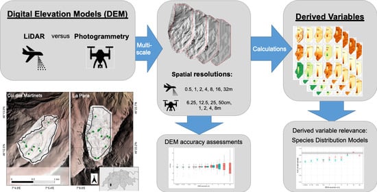
1. Introduction
2. Materials and Methods
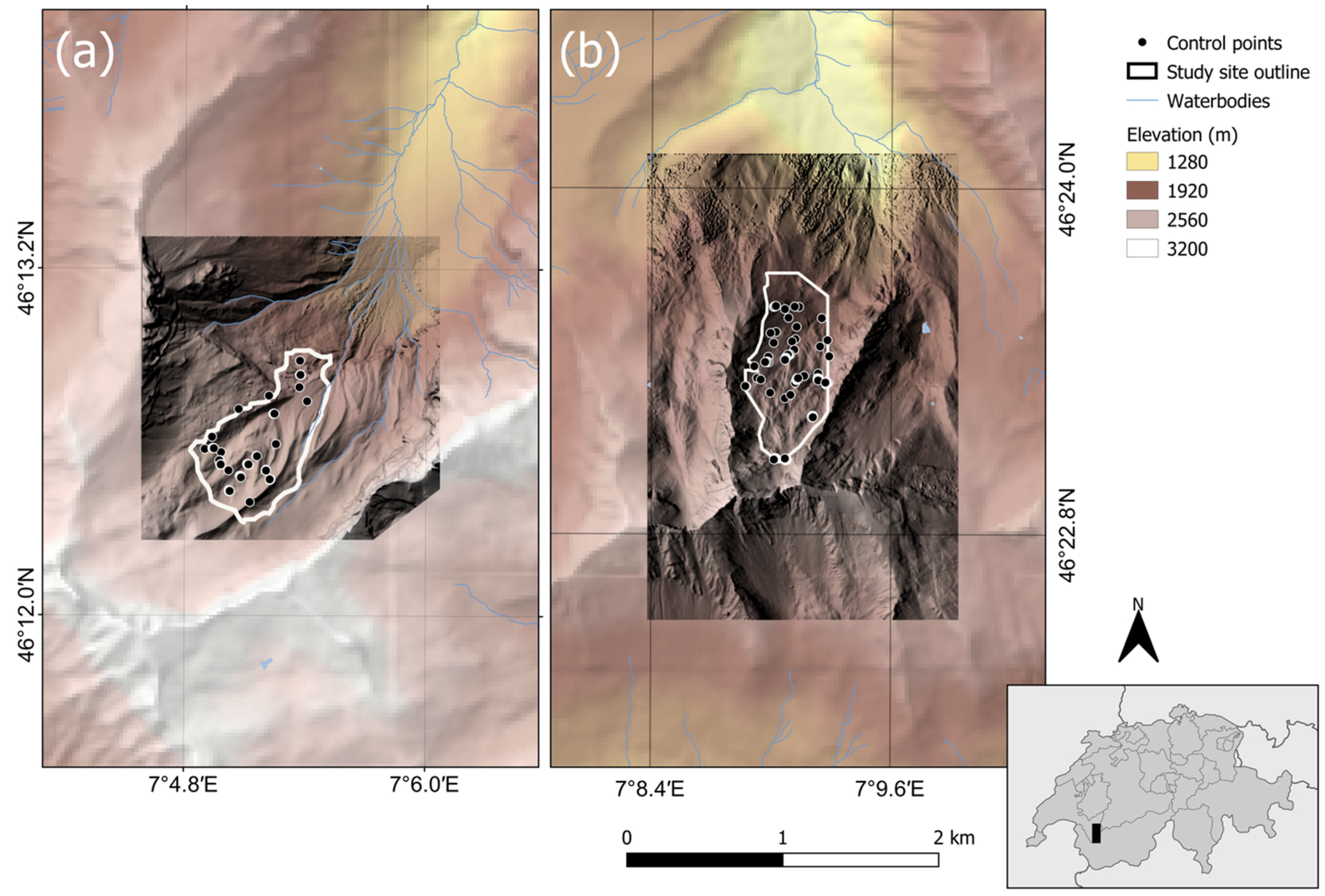
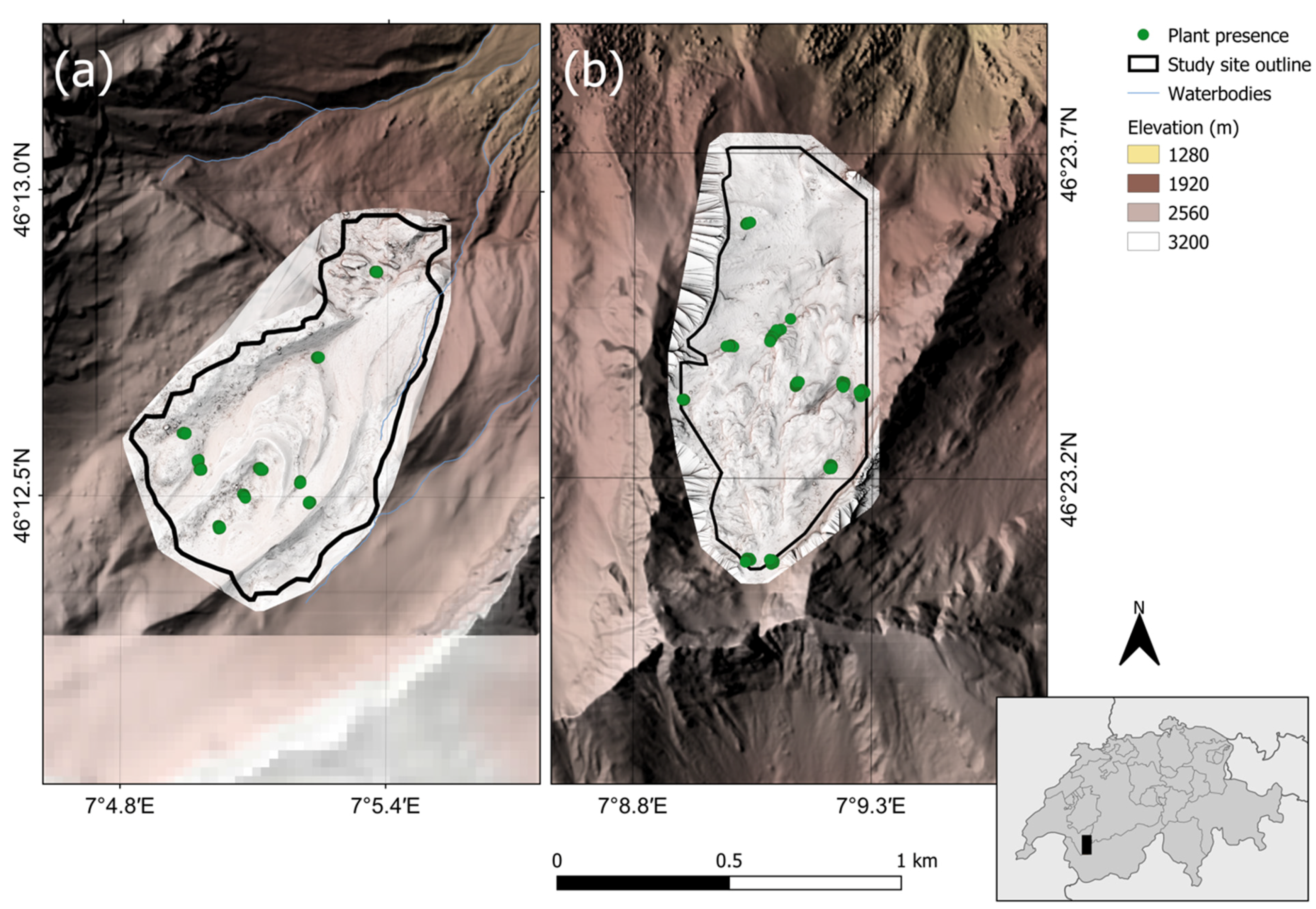
2.1. Study Sites
2.2. Digital Elevation Models
2.2.1. LiDAR Acquisition
2.2.2. Photogrammetry Acquisition
2.2.3. DEM Processing
2.2.4. DEM Multiscale Decomposition
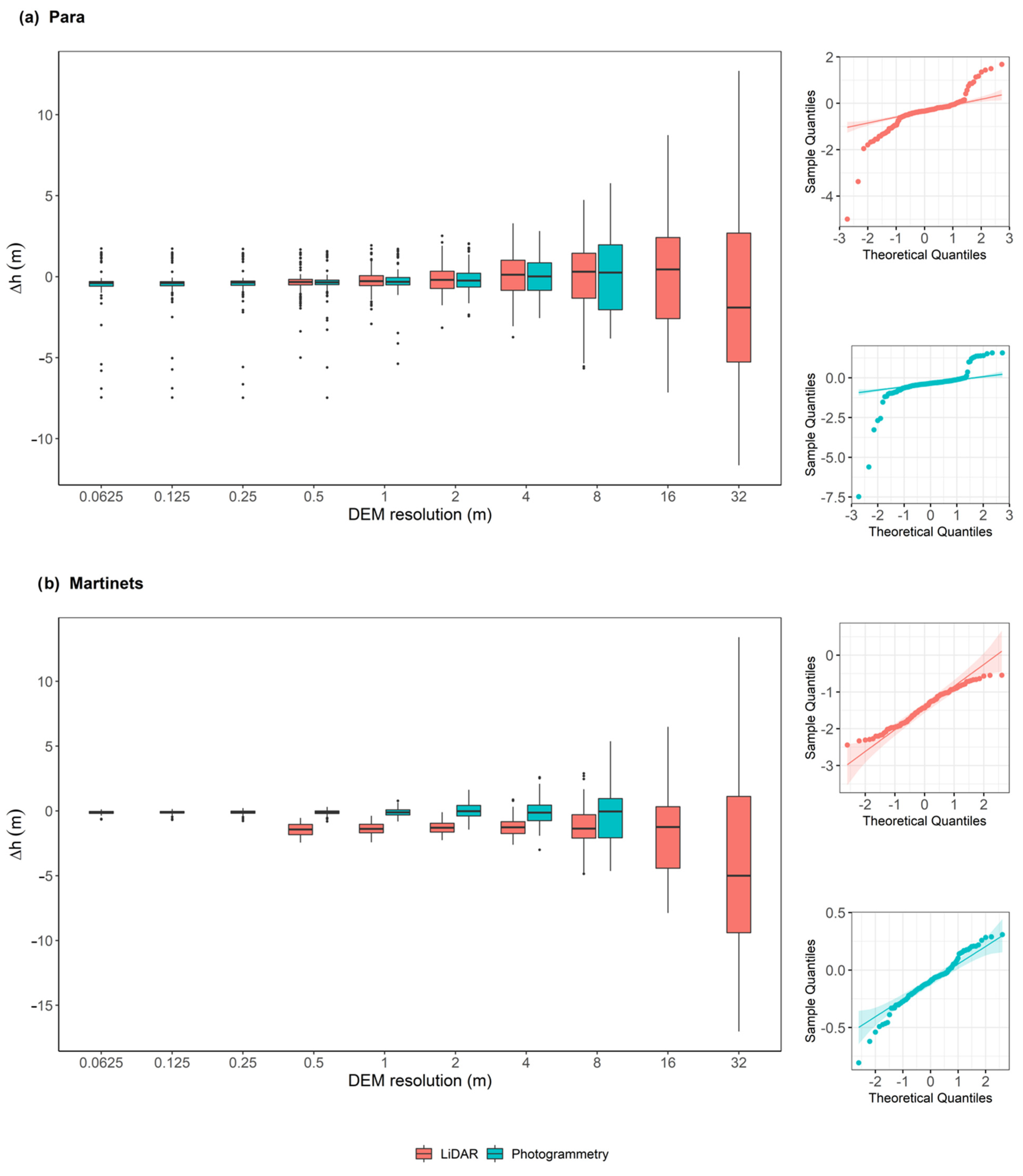
2.2.5. DEM Accuracy Assessment
2.3. DEM-Derived Variables
2.3.1. Derived Variable Computation
2.3.2. Derived Variable Correlations
2.3.3. Derived Variables in Species Distribution Models
3. Results
3.1. DEM Accuracy Assessment
3.2. DEM-Derived Variables
3.2.1. Derived Variable Correlations
3.2.2. Predictive Power of Derived Variables in Species Distribution Models
4. Discussion
4.1. Spatial Scale
4.2. LiDAR Versus Photogrammetry
4.3. Recommendations
4.3.1. Characteristics of the Study Site
4.3.2. Logistics
4.3.3. Environmental Variables
4.3.4. Evaluation
5. Conclusions
Supplementary Materials
Author Contributions
Funding
Data Availability Statement
Acknowledgments
Conflicts of Interest
References
- Inouye, D.W. Effects of climate change on alpine plants and their pollinators. Ann. N. Y. Acad. Sci. 2020, 1469, 1–12. [Google Scholar] [CrossRef]
- Cannone, N.; Sgorbati, S.; Guglielmin, M. Unexpected impacts of climate change on alpine vegetation. Front. Ecol. Environ. 2007, 5, 360–364. [Google Scholar] [CrossRef] [Green Version]
- Gottfried, M.; Pauli, H.; Futschik, A.; Akhalkatsi, M.; Barančok, P.; Benito Alonso, J.L.; Coldea, G.; Dick, J.; Erschbamer, B.; Fernández Calzado, M.R.; et al. Continent-wide response of mountain vegetation to climate change. Nat. Clim. Chang. 2012, 2, 111–115. [Google Scholar] [CrossRef]
- Walther, G.; Beisner, S.; Burga, C.A. Trends in the upward shift of alpine plants. J. Veg. Sci. 2005, 16, 541–548. [Google Scholar] [CrossRef]
- Guisan, A.; Theurillat, J.-P. Assessing alpine plant vulnerability to climate change: A modeling perspective. Integr. Assess. 2000, 1, 307–320. [Google Scholar] [CrossRef]
- Scherrer, D.; Körner, C. Topographically controlled thermal-habitat differentiation buffers alpine plant diversity against climate warming. J. Biogeogr. 2011, 38, 406–416. [Google Scholar] [CrossRef]
- Zimmermann, N.E.; Kienast, F. Predictive mapping of alpine grasslands in Switzerland: Species versus community approach. J. Veg. Sci. 1999, 10, 469–482. [Google Scholar] [CrossRef]
- Graae, B.J.; Vandvik, V.; Armbruster, W.S.; Eiserhardt, W.L.; Svenning, J.C.; Hylander, K.; Ehrlén, J.; Speed, J.D.M.; Klanderud, K.; Bråthen, K.A.; et al. Stay or go—How topographic complexity influences alpine plant population and community responses to climate change. Perspect. Plant Ecol. Evol. Syst. 2018, 30, 41–50. [Google Scholar] [CrossRef] [Green Version]
- Oldfather, M.F.; Ackerly, D.D. Microclimate and demography interact to shape stable population dynamics across the range of an alpine plant. New Phytol. 2019, 222, 193–205. [Google Scholar] [CrossRef] [Green Version]
- Slavich, E.; Warton, D.I.; Ashcroft, M.B.; Gollan, J.R.; Ramp, D. Topoclimate versus macroclimate: How does climate mapping methodology affect species distribution models and climate change projections? Divers. Distrib. 2014, 20, 952–963. [Google Scholar] [CrossRef]
- Pauli, H.; Gottfried, M.; Grabherr, G. Effects of climate change on the alpine and nival vegetation of the Alps. J. Mt. Ecol. 2003, 7, 9–12. [Google Scholar]
- Wilson, J.; Gallant, J. Digital terrain analysis. In Terrain Analysis: Principles and Applications; Wilson, J.P., Gallant, J.C., Eds.; John Wiley & Sons: Hoboken, NJ, USA, 2000; pp. 1–27. [Google Scholar]
- Lecours, V.; Devillers, R.; Simms, A.E.; Lucieer, V.L.; Brown, C.J. Towards a framework for terrain attribute selection in environmental studies. Environ. Model. Softw. 2017, 89, 19–30. [Google Scholar] [CrossRef]
- Böhner, J.; Antonić, O. Land-surface parameters specific to topo-climatology. In Developments in Soil Science; Hengl, T., Reuter, H.I., Eds.; Elsevier: Amsterdam, The Netherlands, 2009; Volume 33, pp. 195–226. [Google Scholar]
- Leempoel, K.; Parisod, C.; Geiser, C.; Daprà, L.; Vittoz, P.; Joost, S. Very high-resolution digital elevation models: Are multi-scale derived variables ecologically relevant? Methods Ecol. Evol. 2015, 6, 1373–1383. [Google Scholar] [CrossRef]
- Frau, L.J.; Libohova, Z.; Joost, S.; Levasseur, C.; Jeangros, B.; Bragazza, L.; Sinaj, S. Regional investigation of spatial-temporal variability of soil magnesium—A case study from Switzerland. Geoderma Reg. 2020, 21. [Google Scholar] [CrossRef]
- Lassueur, T.; Joost, S.; Randin, C.F. Very high resolution digital elevation models: Do they improve models of plant species distribution? Ecol. Model. 2006, 198, 139–153. [Google Scholar] [CrossRef]
- Pradervand, J.-N.; Dubuis, A.; Pellissier, L.; Guisan, A.; Randin, C. Very high resolution environmental predictors in species distribution models: Moving beyond topography? Prog. Phys. Geogr. Earth Environ. 2014, 38, 79–96. [Google Scholar] [CrossRef]
- Leempoel, K.; Duruz, S.; Rochat, E.; Widmer, I.; Orozco-terWengel, P.; Joost, S. Simple rules for an efficient use of Geographic Information Systems in molecular ecology. Front. Ecol. Evol. 2017, 5. [Google Scholar] [CrossRef] [Green Version]
- Lohani, B.; Ghosh, S. Airborne LiDAR technology: A review of data collection and processing systems. Proc. Natl. Acad. Sci. India Sect. A 2017, 87, 567–579. [Google Scholar] [CrossRef]
- Chen, Z.; Gao, B.; Devereux, B. State-of-the-art: DTM generation using airborne LiDAR data. Sensors 2017, 17, 150. [Google Scholar] [CrossRef] [Green Version]
- Liu, X. Airborne LiDAR for DEM generation: Some critical issues. Prog. Phys. Geogr. 2008, 32, 31–49. [Google Scholar] [CrossRef]
- Mlambo, R.; Woodhouse, I.H.; Gerard, F.; Anderson, K. Structure from motion (SfM) photogrammetry with drone data: A low cost method for monitoring greenhouse gas emissions from forests in developing countries. Forests 2017, 8, 68. [Google Scholar] [CrossRef] [Green Version]
- Polat, N.; Uysal, M. An experimental analysis of digital elevation models generated with LiDAR data and UAV photogrammetry. J. Indian Soc. Remote Sens. 2018, 46, 1135–1142. [Google Scholar] [CrossRef]
- Kasser, M.; Delley, N.; Cretegny, S. Comparaison de MNT à haute résolution issus de techniques laser et photogrammétriques. Rev. XYZ 2019, 17–20. (in French). [Google Scholar]
- Baltsavias, E.P. Airborne laser scanning: Basic relations and formulas. ISPRS J. Photogramm. Remote Sens. 1999, 54, 199–214. [Google Scholar] [CrossRef]
- Müller, J.; Gärtner-Roer, I.; Thee, P.; Ginzler, C. Accuracy assessment of airborne photogrammetrically derived high-resolution digital elevation models in a high mountain environment. ISPRS J. Photogramm. Remote Sens. 2014, 98, 58–69. [Google Scholar] [CrossRef]
- Moudrý, V.; Gdulová, K.; Fogl, M.; Klápště, P.; Urban, R.; Komárek, J.; Moudrá, L.; Štroner, M.; Barták, V.; Solský, M. Comparison of leaf-off and leaf-on combined UAV imagery and airborne LiDAR for assessment of a post-mining site terrain and vegetation structure: Prospects for monitoring hazards and restoration success. Appl. Geogr. 2019, 104, 32–41. [Google Scholar] [CrossRef]
- Wu, B.; Tang, S. Review of geometric fusion of remote sensing imagery and laser scanning data. Int. J. Image Data Fusion 2015, 6, 97–114. [Google Scholar] [CrossRef]
- Baltsavias, E.P. A comparison between photogrammetry and laser scanning. ISPRS J. Photogramm. Remote Sens. 1999, 54, 83–94. [Google Scholar] [CrossRef]
- Kasprak, A.; Bransky, N.D.; Sankey, J.B.; Caster, J.; Sankey, T.T. The effects of topographic surveying technique and data resolution on the detection and interpretation of geomorphic change. Geomorphology 2019, 333, 1–15. [Google Scholar] [CrossRef]
- Han, X.; Liu, J.; Mitra, S.; Li, X.; Srivastava, P.; Guzman, S.M.; Chen, X. Selection of optimal scales for soil depth prediction on headwater hillslopes: A modeling approach. CATENA 2018, 163, 257–275. [Google Scholar] [CrossRef]
- Baltensweiler, A.; Walthert, L.; Ginzler, C.; Sutter, F.; Purves, R.S.; Hanewinkel, M. Terrestrial laser scanning improves digital elevation models and topsoil pH modelling in regions with complex topography and dense vegetation. Environ. Model. Softw. 2017, 95, 13–21. [Google Scholar] [CrossRef]
- Lecours, V.; Devillers, R.; Edinger, E.N.; Brown, C.J.; Lucieer, V.L. Influence of artefacts in marine digital terrain models on habitat maps and species distribution models: A multiscale assessment. Remote Sens. Ecol. Conserv. 2017, 3, 232–246. [Google Scholar] [CrossRef]
- Balkenhol, N.; Gugerli, F.; Cushman, S.A.; Waits, L.P.; Coulon, A.; Arntzen, J.W.; Holderegger, R.; Wagner, H.H.; Arens, P.; Campagne, P.; et al. Identifying future research needs in landscape genetics: Where to from here? Landsc. Ecol. 2009, 24, 455–463. [Google Scholar] [CrossRef]
- Anderson, C.D.; Epperson, B.K.; Fortin, M.-J.; Holderegger, R.; James, P.M.A.; Rosenberg, M.S.; Scribner, K.T.; Spear, S. Considering spatial and temporal scale in landscape-genetic studies of gene flow. Mol. Ecol. 2010, 19, 3565–3575. [Google Scholar] [CrossRef] [PubMed]
- Borcard, D.; Legendre, P.; Avois-Jacquet, C.; Tuomisto, H. Dissecting the spatial structure of ecological data at multiple scales. Ecology 2004, 85, 1826–1832. [Google Scholar] [CrossRef] [Green Version]
- Bütikofer, L.; Anderson, K.; Bebber, D.P.; Bennie, J.J.; Early, R.I.; Maclean, I.M.D. The problem of scale in predicting biological responses to climate. Glob. Chang. Biol. 2020, 26, 6657–6666. [Google Scholar] [CrossRef] [PubMed]
- Guillaume, A.S.; Leempoel, K.; Rogivue, A.; Rochat, E.; Kasser, M.; Gugerli, F.; Parisod, C.; Joost, S. Very high-resolution digital elevation models of la Para and les Martinets areas in the Swiss Alps. Zenodo 2021. [Google Scholar] [CrossRef]
- Rogivue, A. Genomic Variation of Arabis alpina (Brassicaceae) in Heterogeneous Alpine Environments. Ph.D. Thesis, ETH Zurich Univeristy, Zurich, Switzerland, 2018. [Google Scholar]
- ASITVD.ch. Available online: https://www.asitvd.ch/ (accessed on 9 December 2019).
- senseFly. eBee X. Fixed-Wing Drone. Available online: https://www.sensefly.com/drone/ebee-x-fixed-wing-drone/ (accessed on 17 February 2021).
- Kalbermatten, M. Multiscale Analysis of High Resolution Digital Elevation Models Using the Wavelet Transform. Ph.D. Thesis, École Polytechnique Fédérale de Lausanne, Lausanne, Switzerland, 2010. [Google Scholar]
- Kalbermatten, M.; Van De Ville, D.; Turberg, P.; Tuia, D.; Joost, S. Multiscale analysis of geomorphological and geological features in high resolution digital elevation models using the wavelet transforms. Geomorphology 2012, 138, 352–363. [Google Scholar] [CrossRef]
- Lee, S.; Wolberg, G.; Shin, S.Y. Scattered data interpolation with multilevel B-splines. IEEE Trans. Vis. Comput. Graph. 1997, 3, 228–244. [Google Scholar] [CrossRef] [Green Version]
- Höhle, J.; Höhle, M. Accuracy assessment of digital elevation models by means of robust statistical methods. ISPRS J. Photogramm. Remote Sens. 2009, 64, 398–406. [Google Scholar] [CrossRef] [Green Version]
- Höhle, J.; Potuckova, M. The EuroSDR test: Checking and improving of digital terrain models. In European Spatial Data Research; Gopher: Utrecht, The Netherlands, 2006; pp. 9–141. [Google Scholar]
- Fischer, M.C.; Rellstab, C.; Tedder, A.; Zoller, S.; Gugerli, F.; Shimizu, K.K.; Holderegger, R.; Widmer, A. Population genomic footprints of selection and associations with climate in natural populations of Arabidopsis halleri from the Alps. Mol. Ecol. 2013, 22, 5594–5607. [Google Scholar] [CrossRef] [PubMed] [Green Version]
- Mod, H.K.; Scherrer, D.; Luoto, M.; Guisan, A. What we use is not what we know: Environmental predictors in plant distribution models. J. Veg. Sci. 2016, 27, 1308–1322. [Google Scholar] [CrossRef]
- Zevenbergen, L.W.; Thorne, C.R. Quantitative analysis of land surface topography. Earth Surf. Process. Landf. 1987, 12, 47–56. [Google Scholar] [CrossRef]
- Sappington, J.M.; Longshore, K.M.; Thompson, D.B. Quantifying landscape ruggedness for animal habitat analysis: A case study using bighorn sheep in the Mojave Desert. J. Wildl. Manag. 2007, 71, 1419–1426. [Google Scholar] [CrossRef]
- Böhner, J.; Selige, T. Spatial prediction of soil attributes using terrain analysis and climate regionalisation. In SAGA—Analysis and Modelling Applications; Böhner, J., McCloy, K.R., Strobl, J., Eds.; Göttinger Geographische Abhandlungen; Goltze Druck: Göttingen, Germany, 2006; Volume 115, pp. 13–27. [Google Scholar]
- Böhner, J.; Köthe, R.; Conrad, O.; Gross, J.; Ringeler, A.; Selige, T. Soil Regionalisation by Means of Terrain Analysis and Process Parameterisation; Micheli, E., Nachtergaele, F., Montanarella, L., Eds.; Research Report No. 7: EUR 20398 EN; European Soil Bureau: Luxembourg, 2002. [Google Scholar]
- Oke, T.R. Boundary Layer Climates; Taylor & Francis: New York, NY, USA, 2000. [Google Scholar]
- Hantzschel, J.; Goldberg, V.; Bernhofer, C. GIS-based regionalisation of radiation, temperature and coupling measures in complex terrain for low mountain ranges. Meteorol. Appl. 2007, 12, 33–42. [Google Scholar] [CrossRef]
- Rochat, E.; Vuilleumier, S.; Aeby, S.; Greub, G.; Joost, S. Nested species distribution models of Chlamydiales in tick host Ixodes ricinus in Switzerland. Appl. Environ. Microbiol. 2020, 1–51. [Google Scholar] [CrossRef] [PubMed]
- Phillips, S.J.; Anderson, R.P.; Schapire, R.E. Maximum entropy modeling of species geographic distributions. Ecol. Model. 2006, 231–259. [Google Scholar] [CrossRef] [Green Version]
- Phillips, S.J.; Anderson, R.P.; Dudík, M.; Schapire, R.E.; Blair, M.E. Opening the black box: An open-source release of Maxent. Ecography (Cop.) 2017, 40, 887–893. [Google Scholar] [CrossRef]
- Elith, J.; Phillips, S.J.; Hastie, T.; Dudík, M.; Chee, Y.E.; Yates, C.J. A statistical explanation of MaxEnt for ecologists. Divers. Distrib. 2010, 17, 1–15. [Google Scholar] [CrossRef]
- Phillips, S.J.; Dudík, M. Modeling of species distributions with Maxent: New extensions and a comprehensive evaluation. Ecography 2008, 31, 161–175. [Google Scholar] [CrossRef]
- Guisan, A.; Graham, C.H.; Elith, J.; Huettmann, F.; Dudik, M.; Ferrier, S.; Hijmans, R.; Lehmann, A.; Li, J.; Lohmann, L.G.; et al. Sensitivity of predictive species distribution models to change in grain size. Divers. Distrib. 2007, 13, 332–340. [Google Scholar] [CrossRef]
- Cavazzi, S.; Corstanje, R.; Mayr, T.; Hannam, J.; Fealy, R. Are fine resolution digital elevation models always the best choice in digital soil mapping? Geoderma 2013, 195–196, 111–121. [Google Scholar] [CrossRef]
- Cook, K.L. An evaluation of the effectiveness of low-cost UAVs and structure from motion for geomorphic change detection. Geomorphology 2017, 278, 195–208. [Google Scholar] [CrossRef]
- Lecours, V.; Brown, C.J.; Devillers, R.; Lucieer, V.L.; Edinger, E.N. Comparing selections of environmental variables for ecological studies: A focus on terrain attributes. PLoS ONE 2016, 11, e0167128. [Google Scholar] [CrossRef] [Green Version]


| Martinets | Para | |
|---|---|---|
| Coordinates | 46°12′37″N; 7°5′12″E | 46°23′23″N; 7°9′6″E |
| Elevation range | 1928–2368 m asl | 1826–2320 m asl |
| Orientation | NE | NNE |
| Slope (mean ± sd) | 0.45 ± 0.17 rad | 0.50 ± 0.16 rad |
| Eastness (mean ± sd) | 0.34 ± 0.6 rad | 0.44 ± 0.5 rad |
| Northness (mean ± sd) | 0.48 ± 0.6 rad | 0.64 ± 0.4 rad |
| VRM 1 (mean ± sd) | 4.7 10−3 ± 9.6 10−3 | 4.5 10−3 ± 7.3 10−3 |
| Area of LiDAR DEM | 3.7 km2 | 6.0 km2 |
| Area of PHOTO DEM | 0.7 km2 | 0.7 km2 |
| Area of target site | 0.5 km2 | 0.5 km2 |
| Ground control points | 13 | 24 |
| Plant occurrence points | 100 | 146 |
| Logger points | 10 | 11 |
| Assessment points 2 | 110 | 157 |
| Variable | Abbv. | Description | Units | Ref. | |
|---|---|---|---|---|---|
| Primary attributes | Elevation | Elev. | DEM elevation, interpolated from LiDAR or PHOTO, generalized to multiple resolutions using B-spline wavelet transforms. | m | [42,43] |
| Slope | Slope | Morphometry. Local morphometric terrain parameters; proxies for water flow, snow movements, erosion, solar radiation, etc. Eastness and Northness represent the sine and cosine of Aspect (Orientation), respectively. Curvature is used to understand erosion and runoff processes. | radians | [50] | |
| Eastness | East | radians | |||
| Northness | North | radians | |||
| Plan curvature | Hcu | 1/m | |||
| Secondary attributes | Vector ruggedness measure | VRM | Morphometry. Quantifies rugosity with less correlation to slope, indicating a combined variability in slope and aspect. | No unit | [51] |
| SAGA wetness index | SWI | Hydrology. Modified version of Topographic Wetness Index (TWI), which is a calculation of the slope and a modified catchment area (MCa). It predicts a more accurate soil moisture for cells situated on the valley floor (when compared to the TWI) | MCa/ Slope | [52,53] | |
| Sky view factor | SVF | Lighting. Ratio of the radiation received by a planar surface to the radiation emitted by the entire hemispheric environment | No unit | [14,54,55] | |
| Total Solar radiation in June | Ti06 | Lighting. Sum of direct and diffuse insolation in summer (calculated for 1 to 30 June 2015). | kWh/m² | [12,14] |
| LiDAR | PHOTO | Pref. | |
|---|---|---|---|
| Data acquisition | |||
| Sensor | Active (laser and sensor) | Passive (images) | Both |
| Vehicle used | Fixed-wing vehicle or helicopter | Drones | Both |
| Flight details | Faster and longer flight, with 20–30% overlap, more complicated flight planning | Slower and shorter flight, with 60–90% overlap, more simple flight planning | Both |
| Area covered | Regional | Local | Both |
| Flight conditions | Light- and weather-independent | Light- and weather-dependent (diffused light to avoid shadows, dry weather, low winds) | LiDAR |
| Terrain type | Suited to most terrain types | Suited to open areas with smooth, visually distinct objects | LiDAR |
| Processing time | Fast/direct | Long/slow | LiDAR |
| Cost | Aircraft: ~US$680–1400/km2 (outsourced service) | Drone: >US$5000 (for complete drone and sensor purchase—acquisition for own use) | PHOTO |
| Software | Open source available (e.g., PDAL); Software licenses start at ~US$150/month (e.g., TerraScan) | Open source available (e.g., MicMac); Software licenses start at ~US$200/month (e.g., Pix4D) | Both |
| Data characteristics | |||
| DEM produced | DTM + DSM 1 | DSM (DTM if little or no vegetation) | LiDAR |
| Data presentation | Monochrome, points only; additional camera can be used for photos | Color and near-infrared images, photos | PHOTO |
| Land classification | Points classified based on reflection and return of laser | Pixels classified later based on point height | LiDAR |
| Data resolution | 50 cm depending on sensor and flight height | 1–3 cm depending on sensor and flight height | PHOTO |
| Feature preservation | May miss some geomorphological features | High performance in preserving geomorphological features | PHOTO |
| Derived variables | Produces more variables | Produces fewer variables due to reduced coverage of surrounding topography | LiDAR |
| Data accuracy | |||
| Accuracy | Better vertical than horizontal | Better horizontal than vertical | Both |
| Characteristics | Accuracy may not be uniform over survey area | More homogeneous within the image format | Both |
| Control points | Low number for validation | High number for photo matching and validation | LiDAR |
Publisher’s Note: MDPI stays neutral with regard to jurisdictional claims in published maps and institutional affiliations. |
© 2021 by the authors. Licensee MDPI, Basel, Switzerland. This article is an open access article distributed under the terms and conditions of the Creative Commons Attribution (CC BY) license (https://creativecommons.org/licenses/by/4.0/).
Share and Cite
Guillaume, A.S.; Leempoel, K.; Rochat, E.; Rogivue, A.; Kasser, M.; Gugerli, F.; Parisod, C.; Joost, S. Multiscale Very High Resolution Topographic Models in Alpine Ecology: Pros and Cons of Airborne LiDAR and Drone-Based Stereo-Photogrammetry Technologies. Remote Sens. 2021, 13, 1588. https://0-doi-org.brum.beds.ac.uk/10.3390/rs13081588
Guillaume AS, Leempoel K, Rochat E, Rogivue A, Kasser M, Gugerli F, Parisod C, Joost S. Multiscale Very High Resolution Topographic Models in Alpine Ecology: Pros and Cons of Airborne LiDAR and Drone-Based Stereo-Photogrammetry Technologies. Remote Sensing. 2021; 13(8):1588. https://0-doi-org.brum.beds.ac.uk/10.3390/rs13081588
Chicago/Turabian StyleGuillaume, Annie S., Kevin Leempoel, Estelle Rochat, Aude Rogivue, Michel Kasser, Felix Gugerli, Christian Parisod, and Stéphane Joost. 2021. "Multiscale Very High Resolution Topographic Models in Alpine Ecology: Pros and Cons of Airborne LiDAR and Drone-Based Stereo-Photogrammetry Technologies" Remote Sensing 13, no. 8: 1588. https://0-doi-org.brum.beds.ac.uk/10.3390/rs13081588