Presenting a Semi-Automatic, Statistically-Based Approach to Assess the Sharpness Level of Optical Images from Natural Targets via the Edge Method. Case Study: The Landsat 8 OLI–L1T Data

Abstract

Developing reliable methodologies of data quality assessment is of paramount importance for maximizing the exploitation of Earth observation (EO) products. Among the different factors influencing EO optical image quality, sharpness has a relevant role. When implementing on-orbit approaches of sharpness assessment, such as the edge method, a crucial step that strongly affects the final results is the selection of suitable edges to use for the analysis. Within this context, this paper aims at proposing a semi-automatic, statistically-based edge method (SaSbEM) that exploits edges extracted from natural targets easily and largely available on Earth: agricultural fields. For each image that is analyzed, SaSbEM detects numerous suitable edges (e.g., dozens-hundreds) characterized by specific geometrical and statistical criteria. This guarantees the repeatability and reliability of the analysis. Then, it implements a standard edge method to assess the sharpness level of each edge. Finally, it performs a statistical analysis of the results to have a robust characterization of the image sharpness level and its uncertainty. The method was validated by using Landsat 8 L1T products. Results proved that: SaSbEM is capable of performing a reliable and repeatable sharpness assessment; Landsat 8 L1T data are characterized by very good sharpness performance.

1. Introduction

The quality of data acquired by spaceborne or airborne sensors depends, in the first instance, on the particular applications for which a specific product was designed and is used. For example, the quality of satellite products exploited for meteorological purposes (i.e., conceived for analyzing large-scale weather-related, atmospheric processes) is evaluated with different criteria with respect to the quality of Earth observation (EO) data used for monitoring small scale environmental and/or anthropic processes (e.g., the impact of natural hazards on urban environments, land use/land cover mapping). Within this context, the reference applications to which the concept of quality is referred to in this paper are those related to the capability of discriminating ground targets in each single band of images acquired by optical EO sensors (e.g., by means of visual analyses). Since these applications can be linked to numerous and different contexts (e.g., environmental monitoring, civil surveillance, etc.), hereinafter, this concept is generally defined as “overall image quality”.

In this framework, the overall image quality depends on several factors, among which the most relevant are the spatial resolution, the radiometric resolution, and the image sharpness [1,2,3,4,5]. Although important, the temporal resolution is not accounted in the abovementioned list because the image quality we are referring to is the one of a single product, without taking into account the added-value provided by the exploitation of a higher temporal resolution to perform multitemporal analyses (e.g., due to the exploitation of constellations of satellites carrying the same sensor). Moreover, even though the spectral resolution is another extremely important factor, it will not be examined in this document. This is due to the fact that the concept of overall image quality considered in this paper refers to the independent quality of each spectral band, without taking into account the mutual relationships existing between the different spectral bands that, in the case of multispectral or hyperspectral analyses, may provide an added-value for discriminating ground targets.

A concise yet exhaustive description of the selected aspects previously listed is reported hereunder to outline the theoretical framework in which the presented research is carried out. In this review, particular emphasis is placed on image sharpness because this paper aims at presenting a statistically-based, semi-automatic approach of sharpness assessment that can be used to evaluate the overall quality of optical images in terms of sharpness. A detailed description of the research objectives of this paper can be found at the end of this first introductive section. The rest of the paper is organized as follows: the methodological description of the proposed approach, including its validation, is described in Section 2. The results of the analyses are then shown in Section 3 and discussed in Section 4, where the possible follow-up activities are also reported. Finally, the conclusions of the study are drawn in Section 5.

1.1. The Most Important Factors Influencing the Overall Quality of Optical Images: A Review

1.1.1. Spatial Resolution

Spatial resolution is one of the most misunderstood and misleading features of remotely sensed data. Within the remote sensing community, its common definition is the minimum size of the targets on the ground that can be resolved (i.e., distinguished) by the sensor. However, in many cases, this interpretation of the concept is not suitable to the wide spectrum of current applications of satellite imagery (see the cases of hot spot detection, sub-pixel mapping, etc.). Thus, the choice of the most suitable metric for representing and measuring this feature is not straightforward as it appears on a first instance [6,7]. Within the scientific community, this topic has been an open question for decades (e.g., [8]), and nowadays, it is still an active field of research (e.g., [9]).

When discussing the concept of spatial resolution of remotely sensed data, it is important to clarify the existing differences between the concepts of spatial resolution and pixel size (PS). The first is an intrinsic native feature of the data (depending on the physical and geometric characteristics of the observing system); the latter depends on the characteristics of the processing applied to the original data (e.g., resampling) that allow displaying the images with a PS equal to or different than the native spatial resolution of the product [10].

Concerning the terminology used for quantifying the spatial resolution concept, it is important to point out that the most widely used metrics are those based on the geometric properties of the imaging system. For all types of EO spaceborne platforms, the full across-track angular coverage is called the field of view (FOV), and the corresponding ground coverage is called the ground-projected field of view (GFOV) (also known as swath width). The angle subtended by a single detector element on the axis of the optical system is called instantaneous field of view (IFOV), whereas its projection onto the Earth’s surface is called ground-projected instantaneous field of view (GIFOV; also known as instantaneous geometric field of view-IGFOV) [1]. The mathematical description of these parameters can be found in [1,5,11], as well as additional details about the topic. End-users of EO-derived products generally prefer to use the term GIFOV. On the other hand, system/sensor engineers prefer the angular parameters IFOV because it has the same values in image and object space [1].

The images derived by EO optical systems are composed of data acquired in a bidirectional sampling process, whose components are defined across-track and along-track. In this process, the along-track platform velocity also plays a role [1]. The distance on the ground in the two scanning directions, known as ground sampling distance (GSD), is another common metric used for defining spatial resolution. The GSD of an instrument can be defined in order to match the GIFOV at nadir. However, the GSD can be made smaller than the GIFOV in the across-track direction to achieve better image quality [1,7]. This can generate further confusion, as highlighted by [7] that raised the following issues representative of the complexity of the topic: “does across-track performance improve just because the data are resampled at smaller intervals compared to IGFOV? Can 5-m IGFOV sensor data, sampled at 1 m, have the same performance as a 1-m IGFOV sensor? What is the maximum allowable ratio of IGFOV over GSD?”

Although from a geometrical and theoretical point of view the spatial resolution can be described by the abovementioned parameters, their values do not necessarily provide the minimum size of objects that can be detectable in an image. In fact, blurring effects due to optic phenomena (e.g., aberration, diffraction) may be present and lead to image degradation. In addition, the nominal IFOV dimension can be degraded because of different (technical/physical) reasons that may reduce the detector size [6]. Conversely, objects smaller than a declared spatial resolution may be sufficiently brighter or darker than their surroundings to change the overall radiance of the pixel and be recognized [6]. In Landsat thematic mapper (TM) imagery, for instance, there can be observed features (such as roads) with widths much smaller than the specified 30 m spatial resolution, providing that there is adequate contrast compared to the surroundings [7].

Other metrics have been developed for quantifying the spatial resolution concept (e.g., Rayleigh diffraction limit-RDL, ground spot size-GSS, Rayleigh resolution criterion-RRC, sparrow metric), but they are less used than the one previously reported. Examples of these metrics can be found in [9], to which the reader is invited to refer for a more detailed explanation.

Finally, a special mention deserves to be reserved to another metric widely used as a standard for quantifying the spatial resolution of an image: i.e., the full width at half maximum (FWHM) of the normalized line spread function (LSF). Because of the strong link of this parameter with another important aspect of the image quality, i.e., the image sharpness-this metric will be extensively described in the following sections of this paper.

1.1.2. Radiometric Resolution

As previously anticipated, other aspects exist that, in addition to spatial resolution, concur to the definition of the overall quality of optical images. Such aspects are not only related to the geometrical properties of the imaging systems but also to the process of data acquisition and image formation, as well as intrinsic sensor characteristics.

When an EO optical sensor acquires data, it integrates the continuous incoming energy (i.e., the electromagnetic radiation), converts it to an electrical signal, and quantizes it to an integer value (the digital number—DN) to store the measurement at each pixel. In this process, a finite number of bits is used to code the continuous data measurements as binary numbers. If Q is the number of bits used to store the measurements, the number of discrete DNs available to store the measurements is 2^Q, so that the resulting DN can be any integer ranging from 0 to DN_max = 2^Q − 1. This range represents the radiometric resolution of the sensor, and the number of bits available to quantize the energy (i.e., Q) is also known as pixel depth. The higher the radiometric resolution, the closer the approximation of the quantized data is to the original continuous signal. However, for scientific measurements, not all bits are always significant, especially in bands with high noise or low signal levels [1].

This last consideration allows us to introduce in the discussion another concept: the signal-to-noise ratio (SNR). Although, to a first-order, an image pixel is characterized by the geometrical properties of the EO acquisition system (e.g., GSD, GIFOV) and by the radiometric resolution, the capability of identifying targets in a digital image also depends on its contrast with the surrounding features (refer to the example of the roads in Landsat TM imagery previously described), in relation to the sensor’s ability to detect small differences in radiance. This is measured by the SNR, which is defined as the ratio of the recorded signal to the total noise present [1,6,12]. A common, simple way to estimate the SNR is given by the ratio between the mean of the signal and its standard deviation [13], computed over homogeneous areas [14]. However, several and more complex alternative strategies have been developed to measure this parameter: e.g., as a function of land cover type and/or wavelength; or by using specific targets such as highly contrasting features such as edges, via the edge method (EM) [14,15]. Therefore, some authors also pointed out the need to have a standardized methodology for SNR assessment that can enable a fair comparison when comparing results provided by different sources [12].

1.1.3. Image Sharpness

Image sharpness is a terminology used as an opposite of image blur, which limits the visibility of details. Most of the image blur is introduced during the acquisition time by both the optical system and the potential motion of the sensor [15].

Image sharpness can be measured by the point spread function (PSF), which describes the response that an electro-optical system has to a point source [16]. Indeed, a digital image can be defined as a collection of object point sources modulated by the intensity at each object location. Each of these object points becomes blurred when viewed by an electro-optical sensor, owing to optical aberrations, sensor motion, finite detector size, diffraction, and atmospheric effects. The PSF is approximately independent of position across a region of the acquisition system’s field of view, and the sharper it is, the sharper the object will appear in the system output image [16]. However, in practice, the direct estimation of the image PSF can be a complex task [6]. Therefore, point targets are not widely used to estimate image quality [16].

Within this context, another important image parameter commonly measured is the LSF, which results from the integration of the PSF. Physically, the LSF is the image of a line or a line of points. The LSF can also be expressed as the derivative of the Edge Spread Function (ESF), which is the response of an electro-optical system to an edge or a step function. In practical terms, this corresponds to regions of the image where a sudden shift in DN is registered. To summarize, in optical terminology, the PSF is the image of a point source, the LSF is the image of a line source, and the ESF is the image of an edge source. From a theoretical point of view, the imperfect imaging behavior of any optical system that results in image blur can be detected and represented using any of these functions. [1]. On the other hand, depending on the specific application and its associated operational issues/challenges, one function may be more suitable than the others.

As previously described, the measurement of the two-dimensional PSF is complicated and requires laboratory measures or a special array of concave mirrors, making its use for quality monitoring analyses complicated. Instead, for such purposes, the estimation of the one-dimensional function LSF (and ESF) is simpler and can be obtained with on-orbit methods (i.e., directly applied to satellite-derived images), such as the EM. The latter, also known as “knife EM” or “slanted EM”, is one of the most widely used approaches for sharpness assessment that, as previously described, could also be used for SNR estimation via edge targets [12,15,17,18]).

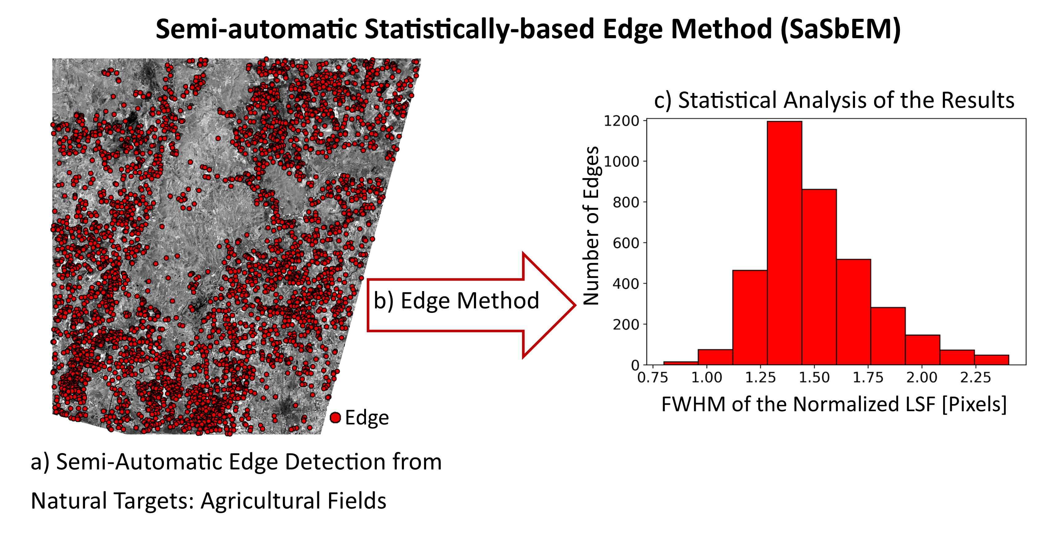
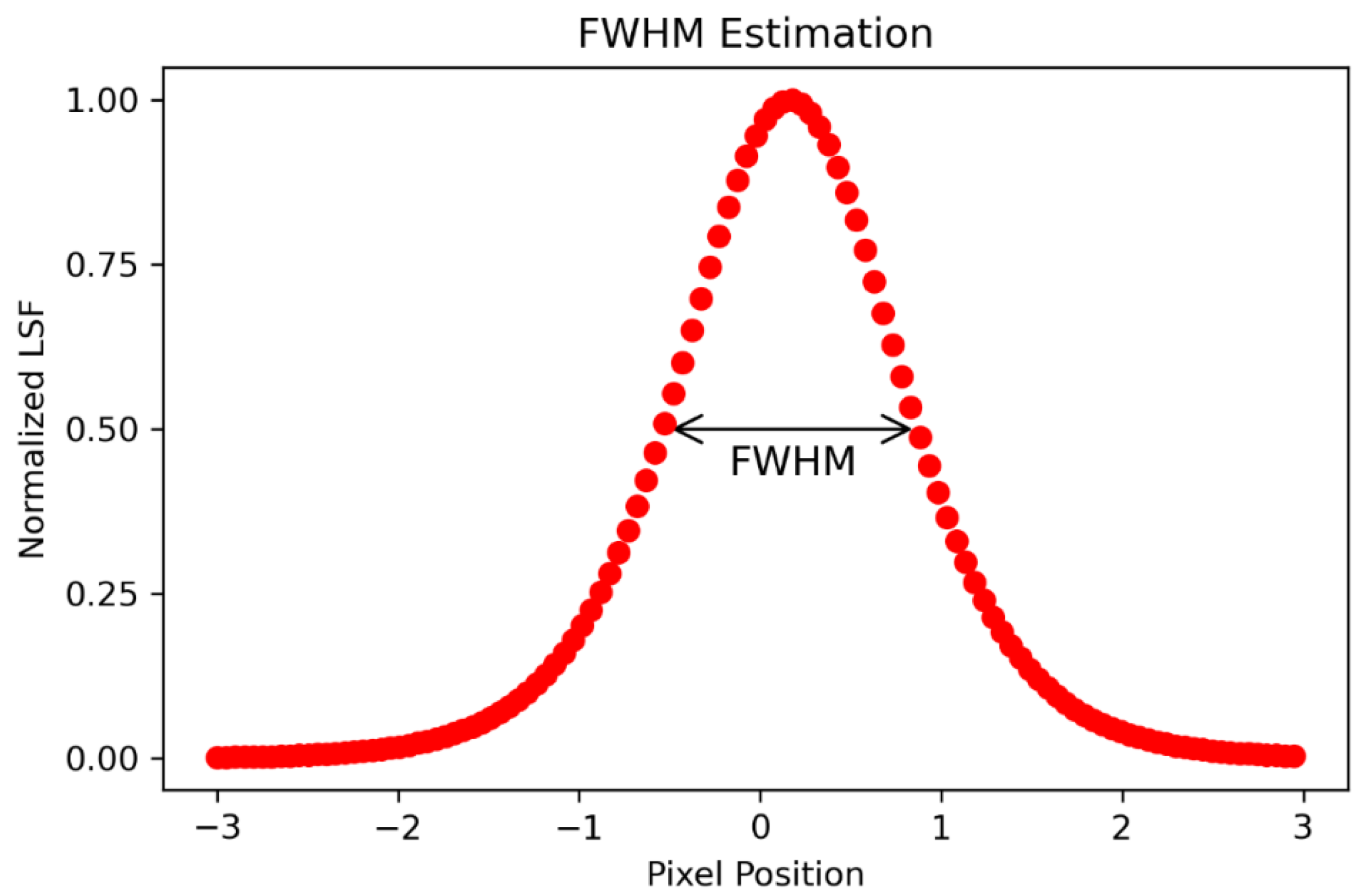
An important metric that can be used to quantify the sharpness level of an image acquired by optical sensors via the EM is the FWHM of the normalized LSF (hereinafter, the term FWHM will be referred to this parameter) [9,12,14,16,18]. The latter is calculated by measuring the width of the normalized LSF at a value of 0.5, as shown in Figure 1 [9,14,16,18]. Therefore, smaller values of FWHM correspond to steeper slopes of LSFs, which in turn are associated to sharper images [16]. The FWHM value is expressed in pixels, and it can then be translated to metric units by taking into account the image PS. Consequently, it can also be used to quantify the effective spatial resolution of the images [9,14,16,19]. Indeed, and as previously anticipated, the FWHM is also considered de facto a standard metric for the spatial resolution of digital images [9].

Other widely used image sharpness metrics are obtained through the evaluation of the modulation transfer function (MTF), which measures “the change in contrast, or modulation, of an optical system’s response at each spatial frequency” [20]. The MTF is mathematically defined as the Fourier transform of the LSF of an imaging system. Consequently, it is the direct transposition of the LSF in the frequency domain. As such, it carries the same fundamental information. The MTF is usually normalized with respect to its maximum value, and the frequency axis is normalized with respect to the sampling frequency at which the LSF is oversampled [20]. The MTF is most often evaluated at the Nyquist frequency, which is generally defined as half the sampling frequency of a discrete signal processing system and, in the case of imaging systems, it is defined as “the highest spatial frequency that can be imaged without causing aliasing” [20]. Less often, the MTF is evaluated at half the Nyquist frequency and, in some contexts, the normalized frequency value at which the MTF reaches half its maximum value (MTF50) is of interest [20]. In any case, the higher the MTF value, the sharper the image, the greater the aliasing effects [16]. Additional theoretical details about the MTF can be found in [10,12,14,16,18]. Most of the time, the MTF characteristics are measured before the launch. However, since vibrations during the launch and sensor degradation through time may alter its original values, on-orbit MTF determination techniques have been developed. Some of them are based on a comparative approach between test images against others whose MTF is already known. Other approaches, such as those based on the EM, exploit manmade/artificial or natural edge targets imaged by the sensors, from which the ESF and the related LSF are estimated and, subsequently, the MTF is retrieved via LSF Fourier Transformation (see Figure 1) [12,14,16,18].

Image sharpness can also be estimated with an additional metric that can be retrieved by applying the EM: i.e., the relative edge response (RER), that estimates the effective slope of the normalized ESF within ±0.5 pixels of the center of the edge [16,20].

In this complex framework, there exist other metrics conceived for characterizing the image quality by linking the spatial resolution and the sharpness concepts: the effective instantaneous field of view (EIFOV) and the radiometrically accurate IFOV (RAIFOV). The first one is defined as the ground resolution corresponding to a spatial frequency for which the system MTF is 50%. The second one is defined as the ground resolution for which the MTF is higher than 0.95 [7,10].

It is noteworthy to highlight that, within the scientific community, the most used sharpness metrics are the FWHM, the MTF (e.g., at Nyquist frequency), and the RER [9,12,16,20]. All of them can be estimated by using a specific on-orbit workflow: the EM (Figure 1).

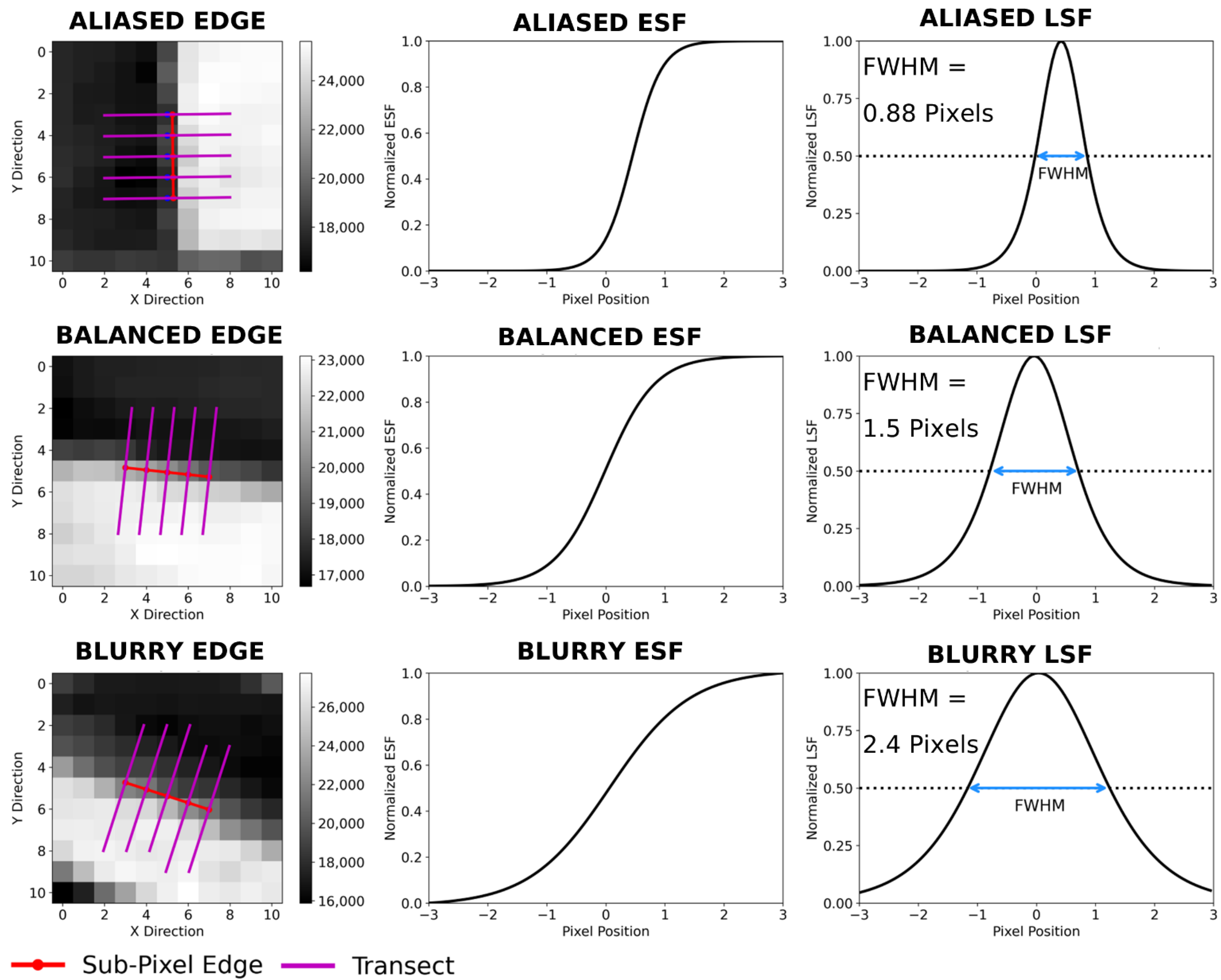
A study ([20]) showed that these three metrics have fixed relationships and that can be used to classify the sharpness level of an image in different categories: aliased, balanced, and blurry. In their work, the authors also provided different examples of these categories of images, as well as different examples of sharpness-related functions and metrics. The reader is thus referred to [20] for having a more detailed description of the topic.

Despite the fact that the EM has some well-known drawbacks (e.g., it can be influenced by the atmospheric effects on the signal recorded by the sensor, its different methodological implementation may lead to significantly different results [12,15], etc.), it is particularly important for monitoring the sensor performances through time. Moreover, if implemented in a standardized manner, it can enable a fair comparison between the sharpness levels of different sensors independently estimated by different entities.

As previously explained, the EM aims at quantifying the sharpness level of an image (i.e., of each single band of the product, in the case of multiband data such as those acquired by optical multispectral sensors) by directly using the edges present in the scene. Although there exist different implementations of the EM, most of the time, it is composed by the following steps, also reported in Figure 1 [12,14,16,20]:

(a)

Edge detection

(b)

Edge sub-pixel estimation

(c)

Computation of the ESF

(c′)

RER estimation

(d)

Computation of the LSF

(d′)

FWHM estimation

(e)

Computation of the MTF

(e′)

MTF estimation at a specific frequency (e.g., Nyquist)

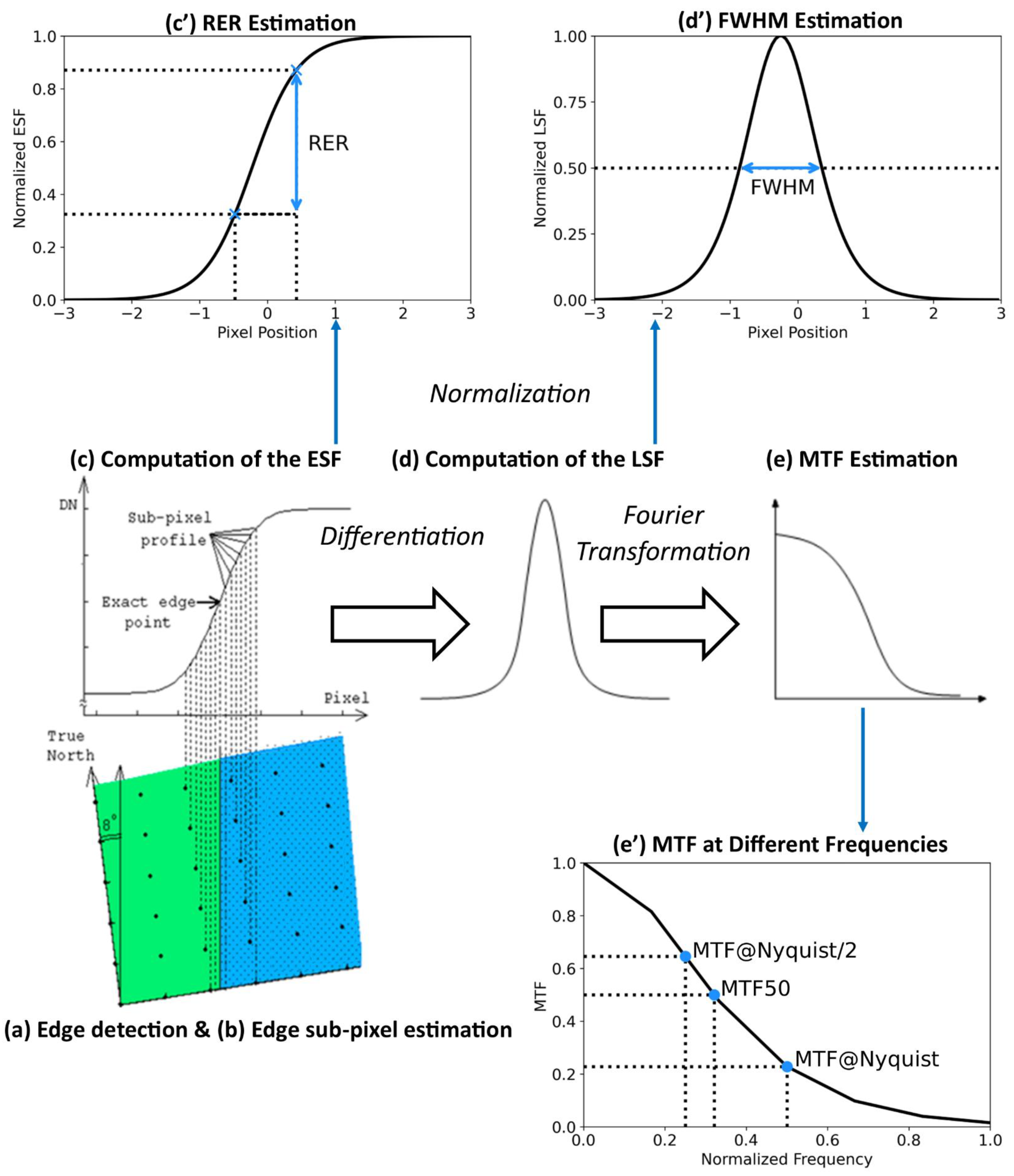
Because the EM results strongly rely on the characteristics of edges selected for performing the sharpness assessment (i.e., the choice of different edges present in the same scene may lead to different results), when implementing this method, one important issue to handle with caution is the definition of the edges to be used for the analysis [14]. Importantly, such edges should also be oriented in multiple directions in order to account for any asymmetries in the PSF when computing the corresponding ESF and LSF [1]. Often, if the sharpness assessment is performed along with specific/preferential directions (i.e., edges oriented along and across the satellite orbit), the overall sharpness level is computed as their geometric mean [9,16]. 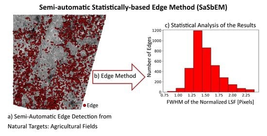Ideal edges are those artificially and specifically built for EM applications (e.g., black and white tarps [16]); nevertheless, images acquired on these specific target areas are not always available. If these targets cannot be clearly resolved by the spatial resolution of the sensor (i.e., the GSD) or images of such areas are not available, different solutions should be explored. One of the most accredited alternatives is based on the definition of the edges by exploiting manmade/artificial (e.g., buildings, runways, roads) and/or natural targets (e.g., agricultural fields, shorelines, canals) [16,17,19,21]. In these cases, most of the time, the edge selection is still performed by a human operator [14,17]. Consequently, the definition of automatic or semi-automatic approaches of edge selection for performing EM-based sharpness assessments from digital images is still an active field of research, not only in the EO domain [22,23,24,25,26].

Although there exist diverse EMs that share the same conceptual framework, their different methodological implementation may lead to different FWHM, MTF, or RER results. Most of the time, this fact prevents a fair comparison among different studies. Consequently, the development of a standard methodology to robustly estimate the EM-derived sharpness metrics should be encouraged [12].

Within this context, another important aspect must be taken into account when comparing the same sharpness metric computed from different images: i.e., their processing level. Indeed, it must be highlighted that the sharpness assessment should be (theoretically) carried out on raw images/data in order to avoid effects and artifacts due to image pre-processing (e.g., orthorectification, resampling) that prevent the evaluation of the ”pure” performance of the instrument used for acquiring the data [9,20]. If raw data are not available, the sharpness assessment should be referred to a specific processing level of the product derived from the sensor under investigation. Importantly, results should be then interpreted accordingly, especially when comparing the outcome of the sharpness assessment against other results obtained by different analyses. The importance of providing quality information at “product level”, in addition to the one provided at “instrument level”, was highlighted by [5].

1.1.4. Composite Indexes

As previously described, the overall image quality depends on several factors that are often interconnected with each other in a complex and non-trivial way. For this reason, efforts have been made to define “aggregated” quality indexes that take into account different quality metrics to provide a single numeric evaluation of the overall image quality. Within this context, a mention shall be reserved for the National Imagery Interpretability Rating Scale (NIIRS), which is a commonly accepted image quality index for panchromatic imagery developed by the U.S. intelligence community [27]. NIIRS was developed for defining the ability to identify certain features or targets within an image with a 10-level rating scale, from 0 (lowest quality level) to 9 (highest quality level) [28]. An image product’s NIIRS rating is typically determined by trained image analysts according to the possibility to identify specific features on the images [16]. A NIIRS rating can also be predicted using the general image quality equation (GIQE) as a function of specific image quality metrics, such as GSD (linked to the spatial resolution), SNR (linked to the radiometric resolution), RER (linked to the image sharpness), and image enhancement (linked to the image processing) [16,29,30]. It is important to point out that GIQE formulation has changed through time, and the reader is invited to refer to [16,29,30] for its accurate description. Although the purpose of this equation has always been the same (i.e., predict NIIRS values), the variety of versions, their subtleties, discontinuities, and incongruences could generate confusion and problems among users when comparing results [2,4,16,29,30].

1.2. Research Objectives

The continuous monitoring of image quality parameters is of fundamental importance for guaranteeing the accurate extraction of reliable information from remotely sensed data and their coherence through time. For this reason, different initiatives, agencies, and services were created to objectively guarantee the quality of the delivered EO data, for instance: the Copernicus Coordinated data Quality Control (CQC) service [31,32,33], the Joint Agency Commercial Imagery Evaluation (JACIE) [34], the Committee for Earth Observation Satellites (CEOS), the Working Group on Calibration Validation (WGCV) [35], etc.

Among the different quality factors that were previously identified and reviewed, the focus of this work is on image sharpness. As explained, one of the most used approaches to assess the sharpness level of optical remote sensing data is via the EM. However, different studies highlighted that EM results may vary, even significantly, if the method is applied even with few methodological differences [12,15]. Moreover, the literature review reported in the previous section of the paper highlighted the importance of selecting suitable edges when applying the EM.

Within this framework, the aim of this paper is to describe a semi-automatic implementation of the EM that was developed to perform a statistically-based sharpness assessment of optical satellite-derived data. For these reasons, the presented approach was defined semi-automatic, Statistically-based edge method (SaSbEM). SaSbEM is also expected to enable a fair comparison among results obtained by the method in different conditions (e.g., different time periods, different locations) and for different instruments/products.

In order to achieve these objectives, an already existing and standardized implementation of the EM (i.e., [14]) was enhanced by developing a semi-automatic procedure of edge selection that allows identifying, in a selected area of the image, all the edges considered suitable for the analyses (i.e., the “eligible” edges) from natural targets: i.e., agricultural fields. The latter are landform features that can be found in abundance in many regions of the world, and their dimension can be resolved by sensors with very different spatial resolutions (i.e., GSD). In order to select these eligible edges in a rigorous, univocal and repeatable way, their characteristics are defined in mathematical terms via predefined criteria that can be adapted to different sensors. The presented method is defined as “semi-automatic” because some crucial steps need to be supervised by an operator in order to correctly perform the analysis, for instance: the selection of the area of the image largely characterized by agricultural landscape to be used for identification of the suitable edges, in case of an image acquired by sensors retaining a large swath width (e.g., in the order of dozens/hundreds of km); the calibration of the eligible edge selection criteria according to the different characteristics (e.g., geometric, spectral, radiometric) of the sensors undergoing the sharpness assessment.

The long-term objective of this study is to lay the foundations for developing a fully automatic statistically-based approach of data quality assessment that can be used operationally for continuous monitoring of the sharpness level of optical data acquired by spaceborne (or airborne) sensors.

The development of this approach was needed for the following reasons. When applying the “conventional” EM, the choice of the most suitable targets to use for carrying out the assessment is a crucial step that strongly affects the final results. As previously explained, there may exist many cases in which the sharpness assessment should be performed on images for which the specific artificial targets (black and white tarps or tribars) are unavailable or for which the sensor’s spatial resolution (e.g., GSD) is not capable of resolving such features. Therefore, one of the alternative approaches that can be adopted is to exploit edges extracted from natural targets, which are abundant all over the globe and can be resolved by sensors with varying spatial resolutions.

Currently, one of the common strategies adopted for detecting suitable edges from natural targets relies on human operators visually inspecting the image, possibly band by band, and selecting the edges to use in the EM [14,17] to perform a per-band analysis. This approach inevitably limits the edge selection to a reasonable number of edges, and the repeatability of the results is inherently dependent on the operator experience. Therefore, possible inconsistencies may arise when comparing results obtained in different analyses. Furthermore, the manual edge selection procedure makes it very cumbersome, if not practically impossible, to carry out large-scale analyses on carried out on a high number of images. This strongly limits the possibility of continuous monitoring of the sharpness characteristics of a certain sensor over time. For these reasons, automatic (and semi-automatic) methods of edge selection aiming at identifying suitable targets to perform an EM-based sharpness assessment were developed [16,36].

Considering all of this, the research described in this paper aims at presenting an existing realization of the EM in which an innovative semi-automatic approach of eligible edge detection was implemented. This enables to carry out a sharpness assessment based on a significant number of eligible edges (e.g., in the order of hundreds) that are selected in a repeatable way: i.e., the edge selection criteria are consistent through space and time. The volume of data generated by carrying out a sharpness assessment based on a large number of edges, as in the SaSbEM case, allows us to analyze the results in statistical terms. This feature permits to perform a robust and reliable sharpness assessment, in which the uncertainty affecting the results can also be estimated. Importantly, SaSbEM was designed in order to be flexible: i.e., to be applied on data acquired by sensors retaining different characteristics (e.g., spatial resolution, radiometric resolution, spectral resolution, etc.). This is paramount for performing a fair comparison across results from different sensors/analyses.

2. Materials and Methods

In this section are reported all the methodological aspects related to SaSbEM. Initially, the arguments supporting the choice of a reference sharpness metric to use for interpreting the results are explained. Subsequently, an accurate step-by-step description of the method is given, with particular emphasis on its innovative features. In this paragraph, the most significant details about the design of the SaSbEM software are also provided. Finally, all the relevant information related to the validation of the results is presented (e.g., the definition of study areas, data sources selection, etc.).

2.1. Definition of a Reference Sharpness Metric for the SaSbEM

As previously explained, the EM allows estimating different sharpness metrics (i.e., RER, FWHM, and MTF), that are expected to provide the same information (i.e., the sharpness level) in different terms. For this reason, [20] identified and quantified their existing relationships. However, other researchers argued that—in some cases—the estimation of the abovementioned metrics could be affected by different degrees of uncertainties, depending on the different methodological implementations of the EM [15,37]. Consequently, the abovementioned relationships could be altered. Indeed, [15] showed that, by applying different EMs, larger differences and errors could be found in the retrieval of the MTF (at a Nyquist frequency) rather than the FWHM. Moreover, they highlighted that the magnitude of these discrepancies may vary even if minor methodological differences (e.g., choice of different interpolation algorithms/oversampling procedures) are present. For these reasons, it was decided to select the FWHM as a unique sharpness metric to be used as a reference for the SaSbEM.

Since the theoretical review that was carried out in the previous section highlighted that the FWHM and the MTF at Nyquist frequency are the two EM-derived sharpness metrics mostly used by the scientific community [9,12,16,20], the choice of the abovementioned reference metric for SaSbEM, i.e., the FWHM instead of the MTF, was further motivated by the following reasons:

• Most of the time, the MTF is computed at a single and predefined point of the total function (e.g., the Nyquist frequency). However, images with the same MTF value at the same point of the function can have different MTF curves (i.e., the MTF function can have different shapes). This issue can generate confusion when comparing the sharpness level of different images in MTF terms [7]. On the other hand, the FWHM is assumed to be computed, approximately, on a bell-shaped function and, since it is estimated by taking into account two specific points of the curve, it is expected to provide a more robust estimation of the sharpness level.
• The FWHM is computed in the spatial domain, and it is expressed in pixels or in metric units. Therefore, the FWHM is a parameter that can be more easily interpreted with respect to the MTF, which is computed in the frequency domain. Consequently, the possibility to generate misunderstandings when talking about sharpness in FWHM terms is reduced.

To a lesser extent, the abovementioned considerations are also valid if the FWHM is compared against the RER. Indeed, the difficulties in estimating these metrics can be considered similar (and, in both cases, the complexity of the analysis is lower if compared against the MTF). However, since the FWHM is expressed in pixels or metric units, in our opinion, its “physical” meaning (and, thus, understanding) is more straightforward than the one of RER (and MTF). Considering the exponential growth of the EO market that occurred in the last few years and expected for the forthcoming ones, this aspect is particularly relevant. Indeed, non-expert users are expected to be more familiar with a sharpness level expressed in terms of FWHM rather than RER or MTF.

2.2. Description of the SaSbEM

SaSbEM implementation mostly follows the methodological specifications of the EM developed by [14]. Importantly, in SaSbEM, the original approach (of [14]) was complemented with relevant, methodological improvements mostly related to the semi-automatic edge detection from natural targets (i.e., agricultural fields) and the statistical analysis of the results. As previously anticipated, the former aspect was designed to semi-automate the method, while the latter was conceived for obtaining robust results that can be characterized in statistical terms. As a consequence, not only the sharpness level can be assessed, but also the uncertainty of its estimate.

SaSbEM can be considered composed by the following five steps that are accurately detailed in this paragraph, in which a concise description of the most relevant aspects of the SaSbEM software is also provided.

• Semi-automatic edge detection from natural targets (i.e., agricultural fields)
• Edge sub-pixel estimation
• Computation of the ESF
• Computation of the LSF and FWHM estimation
• Statistical analysis of the results

The method is independently applied to each band of the image; therefore, SaSbEM results are provided separately for each single band. Since the algorithm is strongly based on the methodological approach described in [14], the reader is referred to this paper if any further technical detail is needed (especially concerning steps 2, 3, and 4). Importantly, the images undergoing the sharpness assessment via SaSbEM must be acquired in clear sky conditions (i.e., without the presence of clouds, cloud shadow, and haze) to avoid possible alteration of sharpness value due to atmospheric effects. Moreover, they should be acquired over areas whose landscape is mostly characterized by agricultural fields in order to provide suitable edge targets to the algorithm. As previously anticipated, if these images are acquired over territories characterized by a heterogeneous land cover distribution, it may be required a selection (performed by the user) of subset areas in which the predominant land cover typology is agricultural.

2.2.1. Semi-Automatic Edge Detection from Natural Targets (i.e., Agricultural Fields)

Initially, the Canny edge detection algorithm [38] is applied to the entire image or its selected subset (i.e., independently to each single band of the image/subset). This algorithm belongs to the gradient-magnitude family of algorithms, which is particularly suitable for our purposes since it is very sensitive to quick shifts in the digital number (DN). The Canny algorithm allows to quickly obtain a mask of potential edges in the form of a Boolean array. The array is subsequently scanned by a function that firstly categorizes the edges into along-track (vertically oriented) and across-track (horizontally oriented) and then performs the first batch of geometric eligibility checks on the potential edges, discarding those that are discontinuous and are either shorter or longer than a user-controllable, pre-set length. In fact, the edge length is an important parameter that must be defined before running the algorithm to guarantee that an adequate number of pixels are sampled for each edge to correctly perform the analysis [16]. The possibility of adjusting the target edge length and also the minimum distance between two edges is very important for the flexibility of the algorithm since choosing excessively long edges may introduce noise in the measurement and negatively affect the sharpness assessment. Furthermore, since the ideal edge length may change with the PS, this feature allows the algorithm to be adaptable to different sensors. Moreover, the possibility to select the minimum distance between different edges can reduce the possibility to sample (i.e., select/process) more than one time the same ground target, in case the linear feature from which the edge is extracted is much longer than the predefined edge length. From now on, we will refer to this issue as the “multiple sampling effect”. Since SaSbEM aims at analyzing the results in statistical terms, processing edges extracted from the same feature multiple times should be avoided to prevent the occurrence of bias affecting the final results.

All the edges that pass the geometric checks are then analyzed by a second function which performs statistical eligibility checks that are tailored to select ideal targets for sharpness assessment.

The ideal edge should have the following characteristics [14,16]:

• There should be a quick transition between the bright and dark areas located nearby the edge;
• The bright and dark areas adjacent to the edge should be individually homogeneous;
• There should be a significant separability between the statistical population of the DN in the bright and dark areas located nearby the edge.

In order to guarantee the coherence and the repeatability of the method, in SaSbEM, these criteria are translated into the following mathematical relationships:

$${\overline{DN}}_{bright}>\alpha ·{\overline{DN}}_{dark}$$

(1)

$$\sigma \left(D{N}_{bright}\right)<\beta ·\sigma \left(D{N}_{grid}\right)$$

(2)

$$\sigma \left(D{N}_{dark}\right)<\beta ·\sigma \left(D{N}_{grid}\right)$$

(3)

$$P_{10}\left(D{N}_{bright}\right)>\gamma ·P_{90}\left(D{N}_{dark}\right)$$

(4)

where $D{N}_{bright}$ and $D{N}_{dark}$ represent, respectively, the arrays that contain DN values in the bright and dark side of the edge, ${\overline{DN}}_{bright}$ and ${\overline{DN}}_{dark}$ their arithmetic mean, $D{N}_{grid}$ contains the DN values of the whole grid around the edge, $P_{10}\left(D{N}_{bright}\right)$ represents the 10th percentile of the $D{N}_{bright}$ statistical population, $P_{90}\left(D{N}_{dark}\right)$ represents the 90th percentile of the $D{N}_{dark}$ statistical population. The band-dependent, dimensionless coefficients $\alpha ,\beta ,\gamma$ need to be calibrated in order to guarantee that the statistical populations of the dark and bright side areas have the previously described characteristics. It is important to point out that, at the moment, the calibration of the $\alpha ,\beta ,\gamma$ coefficients (that may vary according to the different sensor under examination) is performed manually, with a trial-and-error approach aimed at guaranteeing the compliancy of the selected edges to the characteristics of the ideal one. The latter is defined according to user preferences. Therefore, this step, which is crucial for the method, strongly relies on the user experience. On the one hand, this fact can be seen as a drawback of the presented approach because the calibration phase can be time-consuming, and its implementation prevents the presented method from being defined as fully automatic. On the other hand, it has the important advantage to allow the users to have strong supervision on the method and, thus, on the quality of the results. Moreover, once the $\alpha ,\beta ,\gamma$ coefficients are defined for every band of a given sensor, they can be used in all the analyses in which these sensor’s bands are used, drastically reducing the time required for performing large-scale analyses on several data.

The (1) statistical check aims to select the edges whose bright side is significantly brighter on average than the dark side, excluding those which are not contrasted enough. The (2) and (3) checks are conceived to verify that the dark and the bright sides of the edge are much more homogeneous than the whole grid that contains them and the edge. Finally, check (4) aims to control the separability of the statistical population of the DN belonging to the dark and bright areas.

Only the edges that pass all the checks are classified as eligible and are used in the following steps of the SaSbEM.

An example of eligible and not eligible edges detected by SaSbEM is shown in Figure 2.

2.2.2. Edge Sub-Pixel Estimation

Estimating the exact edge location with sub-pixel precision is fundamental to reconstruct precisely the edge profile. This step is performed on the edges that meet all the geometric and statistic eligibility criteria. For each edge, a grid containing the corresponding bright and dark areas located contiguously to the edge is initially defined. The dimension of the bright and dark grid containing the edge varies according to the edge length. More precisely, the grid is centered on the edge and has a square shape. The sides of the grid have a length equal to one of the edges, plus six pixels. The additional six pixels are needed to sample three pixels on either side of the edge in order to account for all the possible edge positions and orientation inside the grid. Subsequently, the sub-pixel edge position is found by fitting the “original” edge position with a cubic polynomial function, as shown in Figure 3 for a single edge pixel: in addition to the DN of the edge pixel itself, the three abovementioned additional pixels are sampled on both sides of the edge. These seven values are then fitted using a cubic spline function. Once the equation of the cubic spline is known, the position of the sub-pixel edge is then assumed to correspond to the zero-crossing of the second derivative of the fitting function. This process is repeated for each row or column of the grid that contains an edge pixel. Finally, after finding all the refined edge positions in the grid, these new coordinates are fitted linearly to obtain the equation of the edge line (assuming the edge has a linear shape). Once the (linear) equation of the sub-pixel edge is estimated, its exact inclination is computed, and the edge is classified as: “along-track”, “across-track”, or “all inclinations” according to predefined criteria (i.e., ranges of degree). The definition of the range of inclinations that discriminates between along- and across-track edges is important in order to guarantee coherence among these definitions when comparing results of different analyses specifically carried out to perform a sharpness assessment in a specific direction. As such, if needed, this parameter can be defined by the operator.

2.2.3. Computation of the ESF

Once the equation of the edge (with sub-pixel precision) is known, also the equations of the transects can be determined. Transects are lines perpendicular to the edge (Figure 4). Their equations allow the selection of the pixels of the bright and dark grid containing the edge to use for the sharpness assessment via the EM. These values, which are thus defining two new separated dark and bright grids surrounding the edge, are obtained by using the DN of the pixels intersected by the transects. Subsequently, these DN values are resampled along each transect by using cubic spline functions to obtain an ESF for each transect. The transects’ ESFs associated with one single edge are then averaged to obtain the final ESF of the edge.

Once the ESF is estimated, two further quality controls are performed to select the suitable edges to use for the sharpness assessment: a goodness-of-fit check and an edge SNR check.

• The former check is performed fitting the averaged ESF with a model function, which is mathematically described by the following equation [14], that can be defined as a modified version of the Fermi function:

$$y\left(x\right)=\frac{a}{1+\exp \left\{\frac{x-b}{c}\right\}}+d$$

(5)

The curve fitting is performed iteratively by using intuitive first-guess values for the coefficients a, b, c, d, that are evaluated in the following order:

-

Coefficient d is simply set to the minimum value of the ESF;

-

Coefficient b is set to the closest integer larger than half the target edge length;

-

Coefficient c is set to −0.5;

-

Coefficient a is set to the central value of the ESF, subtracted by d, and multiplied by two.

Usually, these first-guess values allow the fitting function to converge very quickly, even with relatively strict tolerances. For instance, in the case of Figure 3, the first-guess values are:

-

a = 1929.01

-

b = 3.00

-

c = −0.50

-

d = 9148.29

On the other hand, the converged values are:

-

a = 2286.95

-

b = 4.19

-

c = −0.40

-

d = 9199.48

It is easy to see how the first-guess values are rather close to the final results, boosting the efficiency of the algorithm and reducing the possibility of bad fits. The goodness-of-fit check is then performed by setting a minimum admissible value of the coefficient of determination ($R_{Threshold}^2$) obtained with the fitting function. This is a further innovation with respect to the original version of the method developed by [14], which was thought to improve the quality of the edges that are used for the sharpness assessment. Subsequently, only the modeled (i.e., fitted) ESFs that pass this check are rescaled and normalized using a min-max normalization method (i.e., X_{NormalizedValue} = (X_{OriginalValue} − X_MinValue)/(X_MaxValue − X_MinValue)).

• The latter check on the edge SNR ($SN{R}_{Edge}$) is performed to ensure the reliability of the estimation of the sharpness metrics. It should be noted that the edge SNR is computed using the specification mentioned in [12,15], to which the reader is referred for further details. Please note that the edge SNR should not be confused with the SNR of the whole image. Indeed, it has been shown that sharpness assessment carried out by using edges with relatively low values of SNR may produce results that are significantly different from the true values [15]. In order to account for these aspects, in SaSbEM, the edge SNR value is requested to be higher than a user-controlled pre-set threshold value $(SN{R}_{Threshold}$): i.e., $SN{R}_{Edge}>SN{R}_{Threshold}$. The choice of the $SN{R}_{Threshold}$ value can be based on literature findings (see [12,15,17]).

2.2.4. Computation of the LSF and FWHM Estimation

The LSF is then computed by discrete differentiation of the normalized ESF. Subsequently, its FWHM is obtained (by definition) as the difference (in pixels) between the LSF values at the ordinate 0.5 (i.e., half the maximum value; Figure 5). In the standard configuration of the SaSbEM, only values of FWHM included between 0 and 10 pixels are considered valid (i.e., FWHM values higher than 10 pixels are considered outliers). However, the method allows to change the threshold value according to the user needs; for instance, when a large discrepancy exists between the sensor GSD and the PS of the image (such as for the thermal bands of the L8 thermal infrared sensor—TIRS sensor [17]).

2.2.5. Statistical Analysis of the Results

Once the FWHM is computed for all the eligible edges of all the bands, the statistical population of the results is used to compute a number of metrics useful to quantify the sharpness level of the product under analysis. These statistical parameters are the mean (µ), the standard deviation (σ), and the 5th, 10th, 25th, 50th, 75th, 90th, and 95th percentiles. The µ of the population represents the expected sharpness level of the product under investigation. The σ represents the variability of this estimate (i.e., it measures the dispersion around the mean value). As such, it can be considered a way to estimate the uncertainty associated with the sharpness assessment. These parameters are particularly suitable for statistical populations that are normally distributed (or then can be considered as such, to a suitable degree of approximation). The percentiles are useful to have a more detailed characterization of the results in statistical terms. The 50th percentile (P50) represents the median of the statistical population of the FWHM values. Therefore, it is another indicator useful to evaluate the expected sharpness value of the product under analysis. Differently than the σ, P50 is a metric less influenced by the presence of (possible) outliers. Consequently, it is considered a more robust metric to estimate the sharpness level of the product undergoing the sharpness assessment via SaSbEM. The corresponding measure of dispersion/uncertainty is the interquartile range (IQR), defined as the difference between the 75th and the 25th percentile. Being based on the percentiles, it is a robust measure of variability (i.e., less influenced by the presence of possible outliers than the σ). These parameters are particularly suitable for a statistical population that is not normally distributed (i.e., skewed distributions).

The abovementioned metrics that can be used to quantify the sharpness level of a single image are expected to be computed from dozens to hundreds of eligible edges (depending on the extent of the agricultural areas present in the product undergoing the analysis). However, if an assessment must be carried out to evaluate the sharpness level of a sensor or of a specific processing level generated from its acquisitions, a set of images (e.g., 10 or more) should be analyzed. Then, all the metrics that were previously listed should be computed, separately, for every spectral band, by taking into account all the eligible edges detected in all the images of the dataset. In these circumstances, the statistical metrics are expected to be computed from hundreds to thousands of eligible edges (again, depending on the extent of the agricultural areas present in the products that are accounted for). When performing a similar analysis, it is important that all the images undergoing the sharpness assessment are of the same processing level and that they were acquired in similar atmospheric conditions (i.e., clear sky), over similar target areas (i.e., characterized mostly by an agricultural landscape) and in a restricted time window (e.g., a fixed season of a given year). This is particularly important to avoid possible sharpness differences among the different images of the dataset due to phenological effects (i.e., vegetation growth) and/or sensor degradation through time, which could add noise/uncertainty to the analysis.

In both cases (i.e., a single image or sensor/product level sharpness assessment), SaSbEM results are obtained without any discrimination based on the edge inclinations. Within the presented methodology, these results are classified as referred to as the “all” category, which includes all the edge inclinations. If required by the analysis, the algorithm also computes the abovementioned statistical parameters by taking into account the edge orientations that, as described, can be defined by the user. In such cases, results are also obtained for along-track edges (i.e., edges aligned vertically, along the satellite track) and across-track edges (i.e., edges aligned horizontally, across the satellite track). With this regard, it should be noted that, counterintuitively, the metrics associated with along-track edges refer to its perpendicular sampling direction of DN pixel values. This is due to the fact that the, when using the EM, the sharpness assessment is carried out by analyzing the radiometric transition of transects perpendicular to the edge orientation, as shown by the purple transects in Figure 4 and Figure 6. Obviously, the same concept, in opposite terms, applies to across-track edges. Therefore, if the image space composed by rows (X direction, in a cartesian coordinate system) and columns (Y direction, in a cartesian coordinate system) is used as a reference framework, the following considerations are valid: SaSbEM results referred to the “X” direction category are associated to edges oriented in the along-track direction; SaSbEM results referred to the “Y” direction category are associated to edges oriented in the across-track direction. A visual representation of these concepts is displayed in Figure 6 (first column).

In terms of software design, for each image that is individually analyzed by SaSbEM, the algorithm returns as output:

• An ESRI shapefile containing the georeferenced list of all the eligible edges used for the sharpness assessment. Each record of the list is represented by means of a vector point feature, whose coordinates correspond to the center of the edge (defined at sub-pixel level). All the relevant information required for the statistical analysis of the results are provided for each record: a unique edge ID, the spectral band in which it was mapped, the coordinates (Latitude/Northing, Longitude/Easting) of its central point (expressed in the reference system of the input image undergoing the sharpness assessment), the edge inclination (in degree), the sampling direction category (i.e., All, X, Y) and the FWHM value (expressed in pixel units) associated to the edge;
• A spreadsheet, containing, for each spectral band that was analyzed, the summary statistics of the shapefile data: i.e., the µ, σ, IQR and 5th, 10th, 25th, 50th (i.e., P50), 75th, 90th, and 95th percentiles of the statistical population of FWHM values; the number of eligible edges used for the analysis. This information is provided for each category of sampling direction (i.e., All, X, Y). In the spreadsheet is also present, for each band, the number of edges discarded by applying the $R_{Threshold}^2$ and $SN{R}_{Threshold}$.

When the analysis is carried out on a set of images to perform the sharpness assessment at the product level, the data reported in the single shapefiles of all the images are aggregated to produce a spreadsheet (analogous to the one previously described) containing the summary statistics of the whole dataset.

At the end of SaSbEM analysis, the image or product type sharpness level is numerically represented by an FWHM value, coupled with its corresponding uncertainty measure (i.e., µ and σ; P50 and IQR). The FWHM value is then used to classify the sharpness level in categorical terms by exploiting the following relationships defined by [20]:

• FWHM values lower than 1.0 pixel can be associated with aliased images. Concerning this category: the lower the FWHM value, the higher the aliasing effects present in the image;
• FWHM values ranging between 1.0 and 2.0 pixels can be associated with balanced images. Images of suitable quality, in terms of sharpness, are expected to be included in this category (this range was also confirmed by [2]);
• FWHM values higher than 2.0 pixels can be associated with blurry images. Concerning this category: the higher the FWHM value, the higher the blurring effects present in the image.

Examples of aliased, balanced, and blurry images of edges extracted from natural targets (i.e., agricultural fields) are displayed in Figure 6. The corresponding ESFs, LSFs, and FWHM values are also shown. The figure was generated, via SaSbEM, by using L8 L1T real data acquired in the near-infrared (NIR) spectral band. From Figure 6, it can be observed that: the sharper the image, the steeper the ESF, the narrower the LSF, the lower the FWHM value.

2.2.6. Concise Software Description

SaSbEM was developed by using exclusively the open-source Python 3 programming language, and the code was written entirely by the authors. The software is mostly based on a restricted number of well-known libraries. The most relevant are: Scikit Image, which is used to perform the edge detection via the Canny algorithm; GDAL, which is used to read the input images and to create the output vectors; NumPy and SciPy, which are used to manipulate the arrays and to perform the mathematical operations required by the methodology.

2.3. Validation of the SaSbEM: Methodological Approach

2.3.1. Data Sources and Study Areas

SaSbEM was validated by using twelve L8 images acquired in continental Europe over areas whose landscape is characterized by a predominant presence of agricultural fields.

The L8 satellite payload consists of two instruments, the operational land imager (OLI) and the TIRS. In this exercise, only images derived from the OLI instrument were used. The latter is a push-broom sensor that collects data with radiometric resolution of 12 bits, and a temporal resolution of 16 days, at different wavelengths in the visible (VIS), NIR, and short-wave infrared (SWIR) portions of the electromagnetic spectrum. In these spectral bands, the OLI sensor spatial resolution (i.e., the GSD) and L8 images PS is 30 m. L8 data are also acquired and distributed in a panchromatic band retaining a spatial resolution (i.e., GSD) and an image PS of 15 m. For SaSbEM validation, only the blue (0.450–0.515 µm), green (0.525–0.600 µm), red (0.630–0.680 µm), and NIR (0.845–0.885 µm) bands were used [39].

Because of the wide swath of the L8 images (i.e., 185 km across-track by 180 km along-track [40]), the ground area imaged by the OLI sensor may include a variety of landscapes and targets; although the images were selected in areas characterized by a predominant presence of agricultural fields. This landscape variability may introduce noise during the first step of SaSbEM (i.e., semi-automatic edge detection from natural targets), which is crucial for obtaining reliable results during the sharpness assessment. In order to circumvent this issue, different test areas/subsets (of variable extent) were created in each L8 image used for the algorithm validation. These subsets were identified in areas whose landscape was mainly characterized by agricultural fields and a low percentage of: forest, small urban settlements, and small water bodies (e.g., rivers) (see Figure 7 and Figure 8).

In order to mitigate possible sharpness differences due to different atmospheric conditions, only L8 images retaining a negligible cloud cover percentage were selected for the analysis. Moreover, to avoid possible misclassification errors occurred during the estimation of the cloud cover percentage reported in the metadata, the subsets used for the analysis were identified, by means of a visual inspection of the products, in areas characterized by clear sky conditions (i.e., absence of cloud, cloud shadow, and haze).

For preventing the occurrence of sharpness differences due to possible degradation of the sensor performance through the time windows over which the analysis was carried out, only L8 images acquired in the year 2019 were used.

In order to reduce possible sharpness differences due to seasonal effects on the natural targets (e.g., different phenological conditions), the abovementioned images were selected in a restricted time interval, corresponding to the 2019 (astronomical) summer season.

The full list of the L8 images used for SaSbEM validation is reported in

Table 1. List of L8 images used for SaSbEM validation. For the meaning of the L8 metadata fields reported in the table, refer to [41].

Subset ID	Landsat_Product_ID	WRS_Path/Row	Date_Acquired	Scene_Center_Time	Cloud_Cover
#1	LC08_L1TP_198025_20190627_20190705_01_T1	198/25	27 June 2019	10:34	0.03
#2	LC08_L1TP_198026_20190627_20190705_01_T1	198/26	27 June 2019	10:34	0.00
#3	LC08_L1TP_187026_20190630_20190706_01_T1	187/26	30 June 2019	9:26	0.02
#4	LC08_L1TP_199026_20190704_20190718_01_T1	199/26	4 July 2019	10:40	0.00
#5	LC08_L1TP_200033_20190711_20190719_01_T1	200/33	11 July 2019	10:49	0.03
#6	LC08_L1TP_193024_20190726_20190801_01_T1	193/24	26 July 2019	10:02	0.16
#7	LC08_L1TP_198029_20190729_20190801_01_T1	198/29	29 July 2019	10:35	0.00
#8	LC08_L1TP_202034_20190810_20190820_01_T1	202/34	10 August 2019	11:02	0.01
#10	LC08_L1TP_184033_20190812_20190820_01_T1	184/33	12 August 2019	9:11	0.10
#9	LC08_L1TP_182029_20190814_20190820_01_T1	182/29	14 August 2019	8:57	0.00
#11	LC08_L1TP_202023_20190826_20190903_01_T1	202/23	26 August 2019	10:58	0.03
#12	LC08_L1TP_192029_20190921_20190926_01_T1	192/29	21 September 2019	9:59	0.25

. Their spatial distribution is instead shown in Figure 7 by means of red polygons that represent the different subsets of the images used for the analysis. These polygons are numbered, from #1 to #12, to link Figure 7 and Table 1 (via the field called “Subset ID”). Indeed, in the table are reported the “most relevant” metadata of the products (i.e., the information most relevant with respect to the purposes of the analysis described in this paper).

All the L8 data were downloaded from https://earthexplorer.usgs.gov/ (accessed on 13 April 2021) as L1T terrain-corrected products. This implies that the images are orthorectified products. As previously explained, according to a theoretical point of view, the sensor sharpness assessment should be carried out on raw data to avoid possible alteration of the sharpness level (e.g., due to the application of the resampling algorithm after the orthorectification process). However, the presented works primarily aim at presenting and validating SaSbEM rather than focusing on a rigorous sharpness assessment of the L8 OLI sensor via the analysis of its raw data. As a consequence, the exploitation of L1T data was not considered an impeding factor for their exploitation in this exercise. Importantly, the current analysis based on L8 OLI-L1T data allowed us to perform a sharpness assessment specifically referred to this processing level (i.e., following [5], it is quality information provided at the “product level”).

2.3.2. SaSbEM Implementation

After the L8 data were downloaded, SaSbEM was independently applied to each selected spectral band of the subset area extracted from each image. In order to do so, and as previously explained, the method needs some parameters to be defined. For the current analysis, the following values for the abovementioned parameters were used:

• Edge length: 5 pixels (that, considering the L8 OLI GSD and PS, translates into a ground distance of 150 m);
• Edge minimum distance (from other edges): 10 pixels (that, considering the L8 OLI GSD and PS, translates into a ground distance of 300 m);
• Across-track range of edge inclination: −15 ÷ +15 degrees (an edge orientation of 0 degrees is assumed to be parallel to the Equator);
• Along-track range of edge inclination: −75 ÷ +105 degrees (an edge orientation of 90 degrees is assumed to be parallel to the Greenwich meridian);
• $\alpha ,\beta ,\gamma$ band-dependent coefficients: refer to

  Table 2. $\beta , \gamma$ band-dependent coefficients [-] used for SaSbEM validation.

  	BLUE	GREEN	RED	NIR
  α	1.2	1.3	1.5	1.3
  β	0.25	0.25	0.25	0.25
  γ	1.0	1.1	1.25	1.25

  ;
• $R_{Threshold}^2$: 0.995 [-];
• $SN{R}_{Threshold}$: 100 [-].

Note that the edge length and minimum distance parameter values were defined by taking into account the L8 PS in order to avoid/reduce possible multiple sampling of the same ground feature (e.g., in case of longer, wider agricultural fields). This fact is undesirable because, if it occurs frequently, it can affect the final estimation of the sharpness level (e.g., when computing the mean value). The across and along-track ranges of inclination were set in order to have a reasonable degree of freedom to include a sufficient number of edges oriented toward these two particular directions. As explained, the $\alpha ,\beta ,\gamma$ band-dependent coefficients were obtained after a manual calibration process. The $R_{Threshold}^2$ was selected to ensure the suitable quality of the eligible edges selected to perform the sharpness assessment. The $SN{R}_{Threshold}$ was defined by following the specification of [15].

3. Results

In this section are reported the results of the SeSbEM validation carried out on L8 OLI-L1T data. Consequently, they are described by taking into account both SaSbEM-related methodological aspects and L8-related quality matters. As previously explained, the major innovations of the presented approach concern the first and the last steps of the SeSbEM methodology. Therefore, the findings reported in this section are organized accordingly.

3.1. Semi-Automatic Edge Detection from Natural Targets (i.e., Agricultural Fields)

An example of edges detected by SaSbEM is reported in Figure 8, where a portion of the Subset ID #1 image is depicted. In the figure are shown, by means of point features, the eligible edges selected by the algorithm and used for the sharpness assessment in each spectral band. Every dot corresponds to the central point of an edge with a length of 5 pixels. The dots are displayed in different colors, according to the spectral band in which the edge was mapped.

In

Table 3. In the table are reported the number of edges used for the SaSbEM validation for each spectral band and every category of sampling direction. In addition, also the $SN{R}_{Threshold}$ mean and standard deviation values are reported.

Band—Sampl. Dir.	Number of Edges: Single Subset ID												Tot.	Tot. [%]	Mean SNREdge [-]	St. Dev. SNREdge [-]
	#1	#2	#3	#4	#5	#6	#7	#8	#9	#10	#11	#12
Blue—All	510	136	113	1214	429	1872	265	471	296	733	152	389	6580	100.0	146.1	8.3
Blue—X	69	16	32	288	94	463	58	90	72	152	38	98	1470	22.3	147.7	9.4
Blue—Y	79	23	24	295	137	499	76	55	85	179	48	118	1618	24.6	145.8	8.2
Green—All	607	151	177	1521	460	2272	252	355	183	441	336	318	7073	100.0	146.0	8.3
Green—X	93	16	46	355	113	543	61	69	44	80	71	86	1577	22.3	147.3	9.3
Green—Y	101	25	40	371	129	623	66	35	56	117	94	103	1760	24.9	146.1	8.3
Red—All	965	216	425	4192	476	3318	437	591	447	1197	2177	700	15,141	100.0	146.5	8.2
Red—X	156	23	116	937	121	794	99	109	115	261	498	178	3407	22.5	148.0	9.3
Red—Y	165	45	112	1032	132	903	91	54	116	338	539	228	3755	24.8	146.2	8.2
NIR—All	954	2886	3671	4586	377	1699	180	679	4969	1621	4858	2460	28940	100.0	146.1	8.7
NIR—X	172	388	1004	1021	96	446	32	118	1156	402	1136	585	6556	22.7	147.6	9.9
NIR—Y	182	382	1014	1140	96	430	52	92	1352	481	1370	776	7367	25.5	145.8	8.8

, instead, are reported the number of eligible edges mapped by SaSbEM for every band of each L8 image subsets used for the analysis. The edges are classified according to the following orientation-based categories: “All” the sharpness directions (i.e., all the edges used for the analysis are taken into account, without differentiating according to their orientation); “X”-oriented sampling direction (i.e., edges oriented along-track); “Y”-oriented sampling direction (i.e., edges oriented across-track). In the table are also shown the total number of edges used for the validation, for all the abovementioned bands and categories, in both absolute terms and as a percentage.

3.2. Statistical Analysis of the Results

The outcome of the sharpness assessment carried out on the subsets of the 12 L8 products selected for the analysis is reported below: in

Table 4. SaSbEM validation results for the blue band.

FWHM [Pixels]—Blue Band: Summary Statistics
Metric—Sampl. Dir.	Single Subset ID Statistics												L8 L1T Statistics
	#1	#2	#3	#4	#5	#6	#7	#8	#9	#10	#11	#12
µ—All	1.47	1.47	1.48	1.45	1.43	1.46	1.47	1.43	1.43	1.45	1.42	1.44	1.45
σ—All	0.22	0.20	0.24	0.20	0.19	0.21	0.21	0.20	0.22	0.22	0.22	0.20	0.21
P50—All	1.43	1.46	1.41	1.42	1.38	1.42	1.41	1.39	1.39	1.41	1.41	1.41	1.41
IQR—All	0.28	0.29	0.26	0.24	0.22	0.26	0.26	0.24	0.23	0.29	0.26	0.24	0.26
µ—X	1.44	1.49	1.53	1.41	1.41	1.41	1.43	1.43	1.39	1.41	1.35	1.39	1.41
σ—X	0.22	0.20	0.34	0.21	0.19	0.21	0.19	0.21	0.22	0.25	0.25	0.21	0.22
P50—X	1.42	1.47	1.45	1.38	1.39	1.38	1.41	1.39	1.37	1.39	1.32	1.39	1.39
IQR—X	0.24	0.32	0.33	0.23	0.22	0.26	0.20	0.25	0.22	0.28	0.24	0.25	0.25
µ—Y	1.51	1.50	1.48	1.45	1.42	1.46	1.53	1.49	1.40	1.47	1.43	1.45	1.46
σ—Y	0.24	0.23	0.19	0.20	0.20	0.21	0.21	0.19	0.21	0.20	0.21	0.20	0.21
P50—Y	1.48	1.49	1.48	1.43	1.37	1.42	1.50	1.46	1.39	1.45	1.44	1.42	1.43
IQR—Y	0.29	0.31	0.20	0.24	0.21	0.25	0.34	0.23	0.24	0.26	0.25	0.21	0.26

(for the blue band),

Table 5. SaSbEM validation results for the green band.

FWHM [Pixels]—Green Band: Summary Statistics
Metric—Sampl. Dir.	Single Subset ID Statistics												L8 L1T Statistics
	#1	#2	#3	#4	#5	#6	#7	#8	#9	#10	#11	#12
µ—All	1.47	1.48	1.47	1.45	1.42	1.45	1.46	1.44	1.44	1.46	1.42	1.47	1.45
σ—All	0.23	0.19	0.21	0.21	0.17	0.22	0.20	0.20	0.24	0.23	0.19	0.22	0.21
P50—All	1.42	1.46	1.42	1.41	1.39	1.42	1.41	1.41	1.40	1.43	1.38	1.43	1.41
IQR—All	0.29	0.28	0.24	0.24	0.22	0.26	0.25	0.25	0.23	0.25	0.20	0.28	0.25
µ—X	1.47	1.46	1.44	1.43	1.40	1.41	1.42	1.42	1.46	1.39	1.39	1.41	1.42
σ—X	0.21	0.15	0.20	0.23	0.19	0.23	0.17	0.20	0.24	0.22	0.20	0.26	0.22
P50—X	1.44	1.43	1.41	1.38	1.37	1.37	1.40	1.39	1.41	1.39	1.35	1.40	1.38
IQR—X	0.30	0.10	0.21	0.26	0.23	0.25	0.23	0.23	0.21	0.25	0.14	0.29	0.25
µ—Y	1.52	1.46	1.46	1.45	1.41	1.45	1.53	1.49	1.40	1.49	1.41	1.48	1.46
σ—Y	0.27	0.18	0.22	0.21	0.15	0.22	0.22	0.16	0.22	0.21	0.17	0.21	0.21
P50—Y	1.46	1.43	1.43	1.41	1.40	1.42	1.52	1.49	1.39	1.47	1.40	1.42	1.42
IQR—Y	0.36	0.31	0.22	0.25	0.18	0.26	0.37	0.26	0.20	0.24	0.19	0.24	0.25

(for the green band),

Table 6. SaSbEM validation results for the red band.

FWHM [Pixels]—Red Band: Summary Statistics
Metric—Sampl. Dir.	Single Subset ID Statistics												L8 L1T Statistics
	#1	#2	#3	#4	#5	#6	#7	#8	#9	#10	#11	#12
µ—All	1.47	1.48	1.46	1.45	1.41	1.45	1.47	1.43	1.44	1.45	1.39	1.42	1.44
σ—All	0.23	0.22	0.21	0.20	0.17	0.21	0.21	0.19	0.23	0.22	0.17	0.20	0.20
P50—All	1.43	1.43	1.42	1.41	1.39	1.41	1.42	1.39	1.40	1.42	1.36	1.39	1.40
IQR—All	0.27	0.27	0.26	0.24	0.19	0.26	0.25	0.21	0.25	0.28	0.21	0.24	0.25
µ—X	1.48	1.41	1.41	1.42	1.40	1.40	1.44	1.43	1.42	1.42	1.35	1.35	1.40
σ—X	0.25	0.21	0.21	0.21	0.20	0.22	0.18	0.20	0.26	0.25	0.18	0.21	0.22
P50—X	1.45	1.34	1.39	1.39	1.36	1.37	1.41	1.37	1.36	1.40	1.33	1.34	1.37
IQR—X	0.31	0.23	0.24	0.25	0.23	0.24	0.26	0.23	0.27	0.32	0.20	0.23	0.25
µ—Y	1.52	1.54	1.49	1.45	1.42	1.46	1.50	1.44	1.42	1.45	1.40	1.44	1.45
σ—Y	0.23	0.25	0.20	0.20	0.16	0.21	0.21	0.16	0.21	0.21	0.17	0.19	0.20
P50—Y	1.49	1.49	1.46	1.41	1.41	1.42	1.46	1.42	1.40	1.43	1.38	1.41	1.41
IQR—Y	0.29	0.30	0.25	0.24	0.18	0.27	0.29	0.19	0.24	0.27	0.20	0.24	0.25

(for the red band),

Table 7. SaSbEM validation results for the NIR band.

FWHM [Pixels]—NIR Band: Summary Statistics
Metric—Sampl. Dir.	Single Subset ID Statistics												L8 L1T Statistics
	#1	#2	#3	#4	#5	#6	#7	#8	#9	#10	#11	#12
µ—All	1.48	1.41	1.51	1.45	1.42	1.45	1.47	1.46	1.42	1.44	1.47	1.44	1.45
σ—All	0.22	0.19	0.25	0.20	0.19	0.22	0.20	0.19	0.22	0.22	0.22	0.22	0.22
P50—All	1.44	1.37	1.46	1.42	1.40	1.41	1.44	1.43	1.39	1.41	1.44	1.41	1.42
IQR—All	0.28	0.22	0.31	0.24	0.21	0.27	0.22	0.24	0.25	0.26	0.27	0.25	0.26
µ—X	1.51	1.39	1.48	1.41	1.39	1.41	1.47	1.50	1.38	1.41	1.43	1.38	1.42
σ—X	0.23	0.21	0.26	0.21	0.21	0.23	0.16	0.22	0.24	0.23	0.22	0.23	0.23
P50—X	1.48	1.36	1.43	1.37	1.40	1.38	1.44	1.45	1.35	1.38	1.40	1.36	1.38
IQR—X	0.29	0.24	0.31	0.24	0.25	0.26	0.19	0.31	0.28	0.27	0.26	0.25	0.27
µ—Y	1.48	1.44	1.52	1.45	1.42	1.46	1.51	1.49	1.41	1.43	1.49	1.44	1.46
σ—Y	0.22	0.20	0.26	0.21	0.17	0.22	0.22	0.19	0.23	0.21	0.22	0.21	0.23
P50—Y	1.46	1.40	1.46	1.42	1.40	1.42	1.48	1.48	1.37	1.41	1.46	1.43	1.43
IQR—Y	0.31	0.27	0.31	0.26	0.19	0.27	0.30	0.24	0.26	0.26	0.29	0.27	0.28

(for the NIR band) and in Figure 9 (for all the spectral bands). In all these cases, results are presented by differentiating according to the different orientation of the sampling direction (i.e., “All”, “X”, “Y”).

In Table 4, Table 5, Table 6 and Table 7, results are firstly shown by taking into account the “Single Subset ID Statistics”. These numbers show the main FWHM metrics (i.e., µ, σ, P50, IQR) obtained for each individual subset product. Consequently, they can be used to evaluate the sharpness level of each single portion of the L8 scene (i.e., the subset), which is assumed to be representative of the whole L8 image under examination. Note that these statistical metrics were computed by taking into account the corresponding number of edges shown in Table 3.

In Table 4, Table 5, Table 6 and Table 7, the abovementioned metrics referred to as “L1T statistics” are also reported. These results can be used to evaluate the sharpness level of the blue, green, red, and NIR L8 OLI-L1T product’s bands during the 2019 summer season. In Figure 9, instead, the “L1T statistics” referred to the percentile values are displayed, which are shown to provide a more detailed characterization, in statistical terms, of the L8 OLI-L1T product.

4. Discussion

In this section is reported the discussion of the results. The content is reported in two paragraphs, in agreement with the structure of the previous section.

4.1. Semi-Automatic Edge Detection from Natural Targets (i.e., Agricultural Fields)

As it can be observed from Figure 8, the large majority of edges detected by SaSbEM were found in agricultural fields, as expected. This implies that the definition of the mathematical/statistical criteria used to identify the suitable edges, and the subsequent manual calibration of the required parameters (e.g., $\alpha ,\beta ,\gamma$ band-dependent coefficients), were designed correctly. Only a few edges, instead, were mapped in other categories of natural targets, such as water bodies. More precisely, some of them were found on the shoreline of a river with calm and clear water (e.g., no waves or suspended sediments/matter). These edges were mapped in the NIR band, where the spectral signature of the water is likely to be lower than the surrounding land cover features and, therefore, sharp transitions between these environments can generate edges mapped by SaSbEM in calm and clear water. This consideration is also (particularly) true for edges that can be mapped on shorelines of larger water bodies, such as lakes, seas, and oceans. Although these edges could be detected by SaSbEM only if the target features satisfy the mathematical and statistical conditions predefined by the users, and therefore they can be considered as eligible edges (i.e., valid edges to perform the sharpness assessment), the shorelines’ morphology (i.e., long and continuous feature highly contrasted with respect to the surrounding area) may also produce errors due to the abovementioned multiple sampling effect. For this reason, during the validation of the SaSbEM, the L8 subsets areas were identified in locations in which large water bodies (e.g., seas and oceans) were not present. Possible residual errors induced by the “multiple sampling effect” due to edges mapped along rivers’ shores present in the L8 subset areas (as those shown in Figure 8) were considered negligible, especially if it is taken into account that SaSbEM results are analyzed in statistical terms, and therefore higher relevance is placed on first-order statistical metrics (i.e., µ and P50). Note that the abovementioned considerations referred to the NIR band can be considered valid, to a lower extent, also for the red band, in which the radiometric contrast between the water and the surrounding features is still high (although lower than the one present in the NIR band).

By examining Figure 8, it can also be observed that SaSbEM only detected few eligible edges in urban and forested areas. This is a further demonstration that the definition of the calibration of the mathematical/statistical criteria used to identify the suitable edges was performed correctly. Since SaSbEM results are analyzed in statistical terms, these few edges can be considered outliers and thus are expected to have a negligible effect on the final results.

Another consideration that can be made by observing Figure 8, which, as previously explained, is considered as an exemplifying image representative of the SaSbEM results, is that the number of edges that were detected by the algorithm depends on the spectral band used for the analysis. In fact, the number of eligible edges found by the algorithm increases as the bands’ wavelength increases. Consequently, the higher number of eligible edges was found first in the NIR band, then in the red band. A lower number of eligible edges was instead found in the green and, finally, in the blue bands. This is due to the fact that, according to a radiometric point of view, in the target areas of the algorithm, the NIR and the red bands are more contrasted than in the green and the blue bands (probably due to a combination of atmospheric effect and natural surface spectral reflectance characteristics) [42]. Moreover, possible atmospheric effects (e.g., scattering) are more likely to affect bands acquiring data in the blue (and green) bands.

These considerations are confirmed by the results displayed in Table 3, where it can be observed that SaSbEM is able to detect a large number of eligible edges, in the order of hundreds of edges for the single image analysis and in the order of thousands of edges for the sensor/product analysis. Being the results of the presented method based on a statistical approach, this is an important aspect to point out because it can guarantee a robust and reliable sharpness assessment. Moreover, this is an innovative feature of SaSbEM that differentiates it from the other classical EMs, that strongly rely on the operators’ contribution for the identification and selection of few (up to tens) eligible edges to be used for the analysis (see, for instance, [12,14,17,21]). Nevertheless, this original feature of SaSbEM allows performing large-scale analyses with a minimal contribution of the operator during the edge selection step.

As it can be observed in Table 3, the percentage of eligible edges detected by the algorithm in the X and Y sampling directions is similar and constant across the different spectral bands. This is a further demonstration of the robustness of the SaSbEM, whose numerous statistical and quality checks prevent the algorithm from identifying preferential directions that could introduce biases in the results (e.g., in case the sharpness value of a given sensor differs significantly in one direction with respect to the others).

A further way to evaluate the characteristics of the edges used for the analysis is via the $SN{R}_{Edge}$ parameter. The latter represents a metric capable of quantifying the quality of the edges used for the analysis in radiometric terms. In Table 3 are also summarized, for each spectral band and for every sampling direction, the mean and the standard deviation of the $SN{R}_{Edge}$ values computed by taking into account all the eligible edges mapped in all the images used for the validation analysis. As it can be observed, in all the circumstances, all the mean and standard deviation values are extremely similar. This implies that, on average, the sharpness assessment was carried out by using eligible edges of similar radiometric quality. This is important to avoid the introduction of biases in the definition of the different image or sensor sharpness levels (i.e., different in terms of spectral band and/or sampling direction) due to the selection of edges of significantly different radiometric quality. Indeed, it is remarked that the $SN{R}_{Threshold}$ criterion not only prevents the selection of edges characterized by poor radiometric quality, but it also does not pose any superior limits on the radiometric quality itself.

Since the selection of the suitable edges to use for the sharpness assessment is crucial in SaSbEM (and of all the possible/different implementation of the EMs in general), the future developments of the presented approach will be designed to further enhance this step by automating it. To this aim, ancillary data (e.g., land cover maps) will be exploited to automatically identify, in a given image, the optimal areas characterized by specific targets from which suitable edges can be mapped (e.g., agricultural areas, in the L8 case). This improvement will be particularly relevant to avoid the extraction of eligible edges from sub-optimal targets (e.g., water bodies, urban and forested areas, in the L8 case). Within this context, it must be acknowledged that the definition of optimal target areas from which eligible edges are extracted can be dependent on the sensor/product specific characteristics, mainly the geometric ones: i.e., its spatial resolution (e.g., GSD) and PS. For instance, it is reasonable to think that the optimal target areas for detecting eligible edges to use for the sharpness assessment of very high spatial resolution (VHR) data (e.g., GSD and/or PS ≤ 2 m) can also be associated with artificial targets (i.e., building, runways, roads) [14]. Further research activities are needed to better understand this topic: i.e., the identification of the optimal targets to use for EM-based sharpness assessments carried out on different data characterized by different geometric properties (e.g., GSD and/or PS). Consequently, supplementary analyses are also needed to evaluate the overall SaSbEM performances in such circumstances.

A second improvement of the presented method takes advantage of the (possible) availability of auxiliary quality data of the products under examination (e.g., cloud masks) to mask out areas affected by haze, clouds, and cloud shadows; or to discard images with a low percentage of areas characterized by clear sky conditions. In the validation exercise presented in this paper, these steps were not required because the target areas used for the analysis were visually identified and manually selected at the beginning of the analysis by the operator.

A third follow-up of the presented method will deal with the development of an automatic technique for the calibration of the parameters to be used to perform the sharpness assessment (i.e., the $\alpha ,\beta ,\gamma$ band-dependent coefficients). This last evolution of the method is not trivial because the automatic calibration should be capable of reproducing the user-defined ideal edge by taking into account the specific characteristics of the sensor under analysis, still ensuring the repeatability of the analysis.

These three (possible) enhancements of SaSbEM are thought to enable a fully automatic operational use of the method that, at the moment, is classified as semi-automatic because of the lack of these features.

4.2. Statistical Analysis of the Results

By observing Table 4, Table 5, Table 6 and Table 7 and Figure 9, it can be stated that:

• All the images that were analyzed showed similar µ and P50 values of FWHM, implying that all the scenes have comparable quality performances in terms of sharpness. If the µ and P50 FWHM values are compared against the criteria defined by [20] and [2] and adopted by SaSbEM for interpreting results (see Section 2), it can be stated that all the images used for the analysis have a sharpness level that can be classified as balanced. Indeed, most of the abovementioned values range between 1.4 and 1.5 pixels. The slight difference between the µ and P50 values can be considered negligible for the purposes of the presented analysis;
• The metrics of uncertainty/dispersion, i.e., σ and IQR, provided consistent results throughout the different images that have been analyzed, with most values ranging between 0.2 and 0.3 pixels. This proved the reliability and robustness of SaSbEM. In addition, in this case, the slight difference between the σ and IQR values can be considered negligible for the purposes of the presented analysis;
• The abovementioned considerations are true for all the categories of edge orientation and all the bands;
• No significant differences have been recorded between the sharpness levels of the different spectral bands;
• For almost all the analyzed images, the sharpness performances along the Y sampling direction are slightly worse than the performance along the X direction;
• When observing the L8 L1T statistics, all the aforementioned considerations can be confirmed. Within this context, it is also important to point out that all the “Single Subset ID Statistics” are very similar to the “L1T statistics”. This proves that the L8 OLI-L1T data are consistent and of suitable quality (in terms of sharpness) and that the SaSbEM approach is a reliable method capable of providing coherent results. The good quality performances of the L8 OLI-L1T product can also be appreciated by observing Figure 9, where it is shown that all the L1T statistics’ percentiles have FWHM values ranging between 1.0 and 2.0 pixels (i.e., they are fully comprised within the balanced category, according to the [20] quality classification criteria). The same consideration can be performed by observing the percentiles computed for each single subset (results not shown in this paper);
• It is important to remark, once again, that all the abovementioned conclusions are referred to as orthorectified products (i.e., L8 L1T). According to a theoretical point of view, the sharpness assessment should be carried out on raw data in order to have a characterization of the sensor performance by avoiding artificial alteration of the sharpness level due to pre-processing steps (i.e., data resampling after orthorectification). Although such effects are expected to affect the L8 OLI-L1T products, the results provided by this assessment prove the good quality of the data that were analyzed in terms of sharpness. Moreover, L8 L1T data are largely exploited within the EO community. Therefore, by carrying out a sharpness assessment on these L8 orthorectified products, it is also expected to provide the scientific community with an insightful contribution for characterizing their quality in terms of sharpness.

A detailed comparison of the results obtained in this paper with others available in the scientific literature is difficult to perform because only a few analogous studies were published in peer-reviewed international and scientific journals. Moreover, when performing such comparisons, it must be kept in mind that the different methodological implementations of the approaches used for the analyses may impact the final results [12,15]. Within this complex framework, one research that can be used for performing a comparison is [19], where the authors used an implementation of the EM method to estimate the FWHM of the red band of the L8 OLI sensor by taking advantage of natural targets. Importantly, their analysis [19] used images in cartographic geometry displaying top-of-atmosphere reflectance values. Consequently, their results can be a useful benchmark for comparing the outcome obtained by using SaSbEM because, besides radiometric differences, both levels are referred to as orthorectified data. The reader is referred to the original paper to have a deeper understanding of the methodological differences existing between their analysis and the one presented in this research. According to the findings of [19], the average FWHM of the L8 red band is 1.70 pixels, the corresponding standard deviation is 0.18 pixels, and the edge SNR is 21 [-]. Therefore, also, in this case, the sharpness level can be classified as balanced (according to the classification criteria of [20]). However, the average value reported by [19] is higher than the one retrieved via SaSbEM. The standard deviation values, instead, are comparable. The major differences can be observed in the edge SNR. It is reasonable to think that the differences between the mean FWHM values obtained in the two studies could also be influenced by the lower value edge SNR (i.e., higher FWHM values could be linked to lower edge SNR values). A further study that can provide additional information useful to understand the reliability of the results provided by the presented research is [37], where the authors estimated different sharpness metrics (including the FWHM) via the EM by using Landsat 8 OLI raw data (Level 1R) acquired over the Moon. According to their findings, the FWHM of the blue, green, red, and NIR bands is lower than 1.0 pixel (in the order of ca. 0.73–0.76 and ca. 0.98–0.99, according to different methodological implementations of the EM that were used). This outcome is relevant for the discussion of the results obtained by the analysis described in this paper because it shows how the higher FWHM values obtained by using SaSbEM for analyzing L8 OLI-L1T data could probably be linked to the effect of the orthorectification of the data.

In addition to the abovementioned statements on the L8 validation, the following methodological considerations about SaSbEM can be performed:

• As explained, SaSbEM is based on a standardized EM [14] to which specific methodological improvements were implemented. The presented method has proved to be robust, and its results have proved to be reliable and repeatable. Therefore, SaSbEM is expected to be a valuable tool also to perform comparative analyses of sharpness assessment among different sensor products (of equivalent processing level);
• As shown, the “default” statistical metrics returned by SaSbEM (i.e., µ, σ, the different percentiles, and the IQR) are expected to be sufficient to carry out a robust sharpness assessment of a single product/processing level. However, this does not prevent carrying out a more detailed statistical characterization of the results, if required by the analysis. For instance: the coefficient of variation (CV, defined as σ/µ) can be computed to compare the dispersion of distributions with a different mean (e.g., in case sharpness values of images acquired by different sensors should be compared); the semi-IQR range (defined as half of the IQR value) can be estimated to have a further dispersion metric to use as opposed to the σ; etc. In addition, techniques of statistical inference can be used to further exploit the potential of the large amount of data that can be obtained by using SaSbEM;
• SaSbEM is expected to be a valuable tool for monitoring sensor or product performance over time. This can be achieved by performing the sharpness assessment on a target product type (i.e., on a set of different images of the same processing level, acquired by the sensor) with fixed frequency in time (e.g., annual) for a long time period (i.e., several years), to detect possible deviations of the sharpness level from an initial starting point used as reference.

5. Conclusions

The research described in this paper was thought for developing an enhanced version of an existing, standardized version of the EM [14] that is commonly used to assess the sharpness level of optical EO data. The objectives of the presented approach (named SaSbEM) were two-fold:

• On the one hand, the method was conceived to perform a sharpness assessment by taking into account suitable edges extracted from agricultural fields, which are land features commonly present on Earth. These edges are selected by taking into account specific geometric and statistical criteria defined to uniquely characterize them. This characteristic guarantees the repeatability of the results. SaSbEM, which uses the FWHM as reference sharpness metric, was designed to perform a sharpness assessment either on single products (from which dozens to hundreds of edges can be mapped and used for the analysis) or, more generally, on a specific sensor/processing level (in this case, thousands of edges can be mapped and used for the analysis);
• On the other hand, considering the large number of suitable edges that can be detected by SaSbEM, the presented method was designed to robustly analyze the results in statistical terms. Importantly, this feature allows characterizing their uncertainty.

SaSbEM was validated on a series of 12 Landsat 8 OLI-L1T products acquired in clear sky conditions over agricultural areas during the 2019 summer season. In this exercise, only the blue, green, red, and NIR spectral bands were used. The validation analysis was important to test the SaSbEM performances according to a methodological point of view and to evaluate the sharpness level of the data undergoing the quality assessment. The results of the validation showed that the method is capable of providing reliable and consistent results. In the discussion of the results, possible future developments of the method were also described, which may enable its exploitation as a fully automatic approach that can be used operationally for EO data quality monitoring activities. The presented results also showed that the Landsat 8 OLI-L1T data have very good quality performance in terms of sharpness, retaining an average sharpness level (i.e., FWHM) ranging between 1.4 and 1.5 pixels with an uncertainty ranging between 0.2 and 0.3 pixels for all the bands that were analyzed.

To conclude, it is important to remark that, although very important, sharpness is only one of the features influencing the quality of optical data. Therefore, when the overall quality of a product is evaluated, also other factors should be taken into account (e.g., spatial and radiometric resolutions), as well as their mutual relationships. For instance, future analyses could be aimed at investigating the interdependencies between the nominal spatial resolution of a sensor (i.e., the GSD, the IGFOV), the image PS, the image SNR, image sharpness level, and the overall image quality. Further studies shall be carried out to have a deeper understanding of these topics.