
Canopy Parameter Estimation of Citrus grandis var. Longanyou Based on LiDAR 3D Point Clouds


1
Key Lab of State Forestry and Grassland Administration on Forestry Equipment and Automation, School of Technology, Beijing Forestry University, Beijing 100083, China
2
College of Engineering, China Agricultural University, Beijing 100083, China
*
Author to whom correspondence should be addressed.
Remote Sens. 2021, 13(9), 1859; https://0-doi-org.brum.beds.ac.uk/10.3390/rs13091859
Submission received: 8 April 2021
/
Revised: 28 April 2021
/
Accepted: 6 May 2021
/
Published: 10 May 2021
(This article belongs to the Special Issue 3D Point Clouds for Agriculture Applications)
Abstract
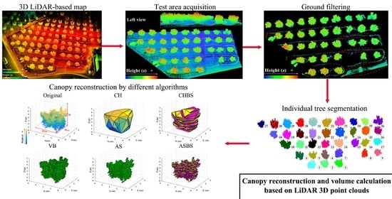
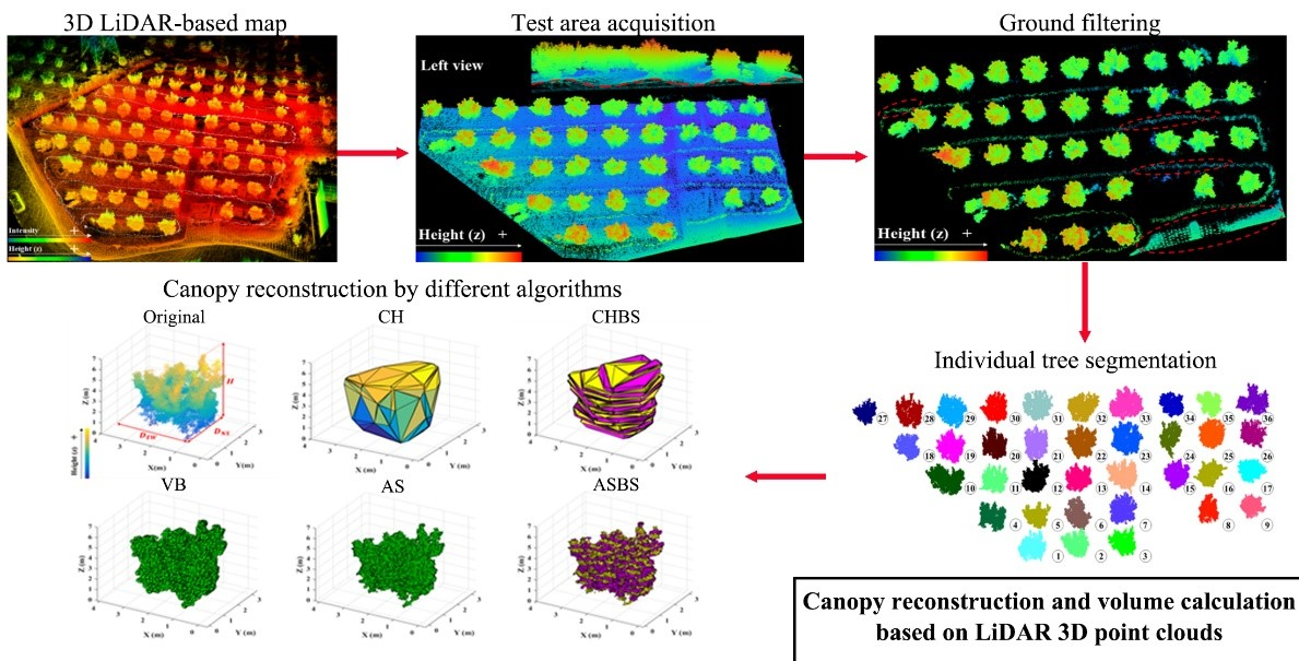
:The characteristic parameters of Citrus grandis var. Longanyou canopies are important when measuring yield and spraying pesticides. However, the feasibility of the canopy reconstruction method based on point clouds has not been confirmed with these canopies. Therefore, LiDAR point cloud data for C. grandis var. Longanyou were obtained to facilitate the management of groves of this species. Then, a cloth simulation filter and European clustering algorithm were used to realize individual canopy extraction. After calculating canopy height and width, canopy reconstruction and volume calculation were realized using six approaches: by a manual method and using five algorithms based on point clouds (convex hull, CH; convex hull by slices; voxel-based, VB; alpha-shape, AS; alpha-shape by slices, ASBS). ASBS is an innovative algorithm that combines AS with slices optimization, and can best approximate the actual canopy shape. Moreover, the CH algorithm had the shortest run time, and the R2 values of VCH, VVB, VAS, and VASBS algorithms were above 0.87. The volume with the highest accuracy was obtained from the ASBS algorithm, and the CH algorithm had the shortest computation time. In addition, a theoretical but preliminarily system suitable for the calculation of the canopy volume of C. grandis var. Longanyou was developed, which provides a theoretical reference for the efficient and accurate realization of future functional modules such as accurate plant protection, orchard obstacle avoidance, and biomass estimation.
1. Introduction
Citrus grandis var. Longanyou is distributed in Guang’an city, Sichuan Province, from the hills of central Sichuan to Huaying Mountain in the east. It is one of the national agricultural products of geographical indication in China; tree shapes include open-hearted, round-headed, and double-layered and Y-shaped [1]. The canopy adsorbs light, interacts with the external environment, and is the main place where fruit trees perform respiration and photosynthesis. Information perception studies have shown that the crown determines the growth and development of trees, which in turn affects their yield and economic benefits [2]. Canopy characteristics have important guiding significance for research related to trees, because they can usually be used for growth assessment [3], biomass estimation [4,5], pruning effect analysis [6], yield prediction [7], health assessment early disease detection [8,9] and in the use of plant protection products such as insecticides [10]. Fruit tree canopy characteristics include canopy height, width, and volume. Among these, canopy volume has an important influence on the nutrient demand and fruit yield of fruit trees [11]. In addition, accurate canopy volume information provides basic data for decisions related to variable spray application, and also affects the precise and variable application of pesticides [12]. Therefore, calculating the geometric parameters of the canopy quickly and accurately is of great significance for the intelligent and accurate management of orchards and plantations.
When precise information about the characteristics of the canopy is acquired, these data can be used for the fixed-point management of crops, thus improving crop yield [13]. At present, methods used to measure canopy volume mainly include manual measurement and various non-contact automatic measurement methods. Manual measurement usually involves collecting canopy height and diameter data for individual fruit trees on site; then, the canopy is treated as a regular solid shape based on the shape of the canopy, and canopy volume is calculated using a formula of approximate regular geometric volume [13]. Because canopy shapes vary from tree to tree, it is difficult to apply a standard uniform and regular geometrical shape to calculate canopy volume, and many researchers have independently proposed standards. Schinor et al. [14] assumed that a fruit tree takes on an ellipsoid shape to calculate the canopy volume. The ellipsoid model is also a common and frequently used geometric model [15,16]. In addition, managers of most Brazilian groves often calculate canopy volume by calculating the volume of a cube surrounding the canopy as the required volume; Scapin adopted this model when studying citrus canopies, independently [17]. Another type has been proposed by Li et al. [18] to measure the circumference at different heights of fruit tree canopies using a tape ruler, and then calculating the area of the circle. The volume of the fruit tree canopy is calculated by the layered volume of the cylinder measured at various heights, and the total volume is the sum of the volume of each layer. This method is more accurate and can reflect the volume of actual fruit trees. Manually measurement using the contact method is simple, easily undertaken, and requires limited mathematical knowledge for growers, but is time-consuming, labor-intensive, and inefficient; in addition, it is easy to damage a tree. Moreover, the accuracy of measurement is susceptible to mismeasurement of subjective factors. The lack of branches in the structure parameters of the system description fails to meet the requirements for an orchard measurement operation [13,19].
Approaches based on photoelectric technology have become the mainstream method used to establish three-dimensional (3D) models of objects without direct contact; this method is now used to study the canopy parameters of fruit trees. Ni et al. [20] reconstructed the canopy structure of Croton, pepper, and lemon using a monocular stereo vision system, whereas Hobart et al. [21] realized the 3D reconstruction of an apple orchard map with a RGB camera and calculated the tree trunk height. Dong et al. [22] used a high-resolution camera to achieve 3D reconstruction of apple and pear trees, and to calculate tree canopy area and diameter. Jurado et al. [23] reconstructed olive tree morphology and estimated plant height and volume using voxel-based methods by incorporating multi-spectral sensors based on high-resolution cameras. The advantages of using cameras and other devices to obtain data are their low cost, easy system development, and access to texture information. The disadvantages are that a camera is easily affected by natural light and post-processing is complicated. The advantages of a depth camera are wide-angle viewing and strong anti-interference ability, which makes up for the defects of cameras and other equipment. Li et al. [24] and Vazquez-Arellano et al. [25] used a depth camera to establish a 3D model of maize plants, and the latter applied it to plant positioning. Zhou et al. [26] realized the 3D reconstruction of the trunks, branches, and canopy of trees indoors and outdoors using a Kinect V2 depth camera, with a method featuring rapid timing and high accuracy. However, the main disadvantage of depth cameras is the low resolution of depth images. As a precision measuring approach, light detection and ranging (LiDAR) has the advantages of rapid image acquisition of 3D point cloud information and high precision, and is not easily affected by the external environment. As a result, it is currently widely used in agricultural production. Medeiros et al. [27] obtained point cloud data with a 2D laser sensor to reconstruct a model of apple trees, and then constructed the skeleton model of fruit trees for pruning. Qiu et al. [28] constructed a 3D map of cornfields and calculated the row spacing and plant height using LiDAR combined with the Global Navigation Satellite System on a mobile platform. Yun et al. [29] selected portable mobile LiDAR to obtain oak data to document hurricane and cold damage in three different sites, and evaluated the sensitivity of different rubber trees to damage from natural disturbance by calculating the included angle between the trunk and primary branches, tree height and canopy volume, and other biological characteristics.
Two methods have mainly been used to calculate canopy volume based on point clouds obtained by LiDAR: The first method involves using triangulation of points outside a point cloud to represent the object surface. This method allows the researcher to form an outer envelope polygon from the outside to the inside of the crown surface, and then calculate the volume. The second method is based on discretization to create small regular geometric or patch models within a point cloud structure [30]. The first method can be divided into two related methods, called convex hull and alpha shape. Xiao et al. [31] used a convex hull algorithm to calculate the volume of sugar beet for predicting biomass, and Lin et al. [32] proposed an improved convex hull algorithm to reconstruct the canopy of 20 trees and calculate the projected area and volume of the canopy, which greatly reduced the time required by the algorithm. Colaço et al. [30] used an alpha-shape algorithm to calculate the canopy height and volume of a commercial citrus orchard. Vauhkonen et al. discussed the application of the alpha-shape algorithm to estimating forest stock volume [33] and proposed an improved alpha-shape algorithm to estimate forest biomass [34]. Wang et al. [35] undertook canopy reconstruction and volume calculation for trees in orchards using the same algorithm. Yao et al. [36] used 2D convex hull and alpha-shape algorithms to calculate forest canopy area and volume, respectively, for the identification of forest tree species. In addition, 3D convex hull and alpha-shape algorithms were used to calculate forest canopy volume for comparison with field-measured values and the ellipsoid canopy volume in the study of Korhonen et al. [15]. The result showed that the estimated value based on LiDAR is usually smaller than the measured value. Jiang et al. [3] also calculated the canopy volume of blueberry bushes for yield assessment using these two algorithms.
Slicing- and voxel-based algorithms are based on discretization. The former borrows concepts from calculus along the horizontal Z-axis, which is split into slices; in turn, the subdivision volume is obtained using other methods, and finally the accumulated canopy volume can be obtained. The latter involves dividing the point cloud of trees into small cubes to reconstruct the trees’ canopy and then calculating the canopy volume. Wu et al. [37] used a voxel-based algorithm to reconstruct street trees, and calculated tree height, crown width, and other parameters. Zhang et al. [38] established a 13A high-spindle-shaped Malus domestica Borkh. digital model. Moreover, a cubic unit segmentation of the model was performed and the light capture rate of various branches in the total canopy and the canopy itself were analyzed. Hosoi et al. [39] established an accurate tree body model based on voxels for Camellia sasanqua and Deutzia crenata, and studied estimation methods used to accurately calculate leaf area density (LAD) and the cumulative leaf area index (LAI) under different conditions. Many researchers integrated the use of a variety of methods to reconstruct the canopy. Olsoy et al. [40] calculated the volume of sagebrush (Artemisia tridentata) by convex hull and voxel algorithms to estimate total and green biomass. Fernández-Sarría et al. [41] used convex hull, convex hull by slices, and voxel-based algorithms for street trees to reconstruct a canopy model and calculate canopy volume. Bi et al. [42] used the same algorithms for the Amorpha canopy to calculate canopy volume and verified that a voxel-based algorithm was most suitable. Cheein et al. [43] calculated the volume of the olive canopy using the same three algorithms compared with a cylindrical fitting model, and analyzed the characteristics of the different methods. Yan et al. [44] proposed another self-adaptive slicing concave-hull algorithm and compared the results with those of a convex hull, convex hull by slices, alpha-shape, voxel-based, and geometric models, which realized the reconstruction and volume calculation of a street tree canopy.
As a national agricultural product of geographical indication in China, published research studies about estimation of the canopy characteristics, and different calculated volume values using different algorithms, of C. grandis var. Longanyou have rarely been reported. In addition, few studies have been published to date on the method of calculating the crown volume by combining the alpha-shape algorithm and slices (alpha-shape by slices), or about comparative analysis based on the quantitative relationship of the calculated volume combined with the running time. In this study, based on 3D point cloud data collected by LiDAR, canopy point clouds of fruit trees were obtained by filtering and single tree segmentation. The existing manual method (MM) and five canopy reconstruction algorithms based on point clouds (APCs, specifically convex hull, CH; convex hull by slices, CHBS; voxel-based, VB; alpha-shape, AS; alpha-shape by slices, ASBS) were compared and analyzed by calculating results and determining the run time required for analysis. The relationship between different volume values is explored, and suitable algorithms are proposed for different job requirements. We calculated crown volume by combining the alpha-shape algorithm and slices (alpha-shape by slices, ASBS), and in this paper discuss the relationship among different algorithms. It was found that ASBS can better remove internal holes and gaps, and more closely approach the real canopy shape. Furthermore, VASBS can be calculated indirectly using a CH algorithm with the shortest running time via good quantity relationships. In addition, suitable algorithms are proposed for different job requirements. The six calculation methods shown in this work provide canopy-related geometry in addition to theoretical references designed to support intelligent orchard management in the future. The research method adopted in this study is described in Section 2. The discussion of Section 3 combines the calculation results and algorithm principles to conduct an in-depth analysis, discussing the reasons for the results and the main findings of this research. Section 4 summarizes the relationship among the volume values of different algorithms of C. grandis var. Longanyou and the optimal algorithms for different work requirements; it also emphasizes the potential contribution of this study and the improvements needed in future research.
2. Materials and Methods
2.1. Test Area and Test Equipment
The test site was a grapefruit plantation in Guang’an city, Sichuan Province, China. Citrus grandis var. Longanyou trees were used with row spacing of 5–6 m, plant spacing of about 6 m, and a tree height of about 4 m. The branches at the top are of different heights and diverge to both sides, and the branches of adjacent trees intersect each other inside, resulting in numerous holes and gaps between branches and leaves. The open-hearted shaped trees were cultivated using the ridge-tillage cultivation method; the ridge spacing is 5–6 m and the ridge height is 0.4–0.5 m. The experiment was conducted in Guang’an township, Guang’an district, Guang’an city in 2019. The local (30°50′ N, 106°76′ E) average elevation is 320 m, and the annual average temperature is 17.58 °C. The test site is in a typical hilly area of southwest China with high temperatures, a rainy climate, and medium soil fertility. A total of 36 grapefruit trees in five rows were selected as test samples in this experiment; the test scene is shown in Figure 1.
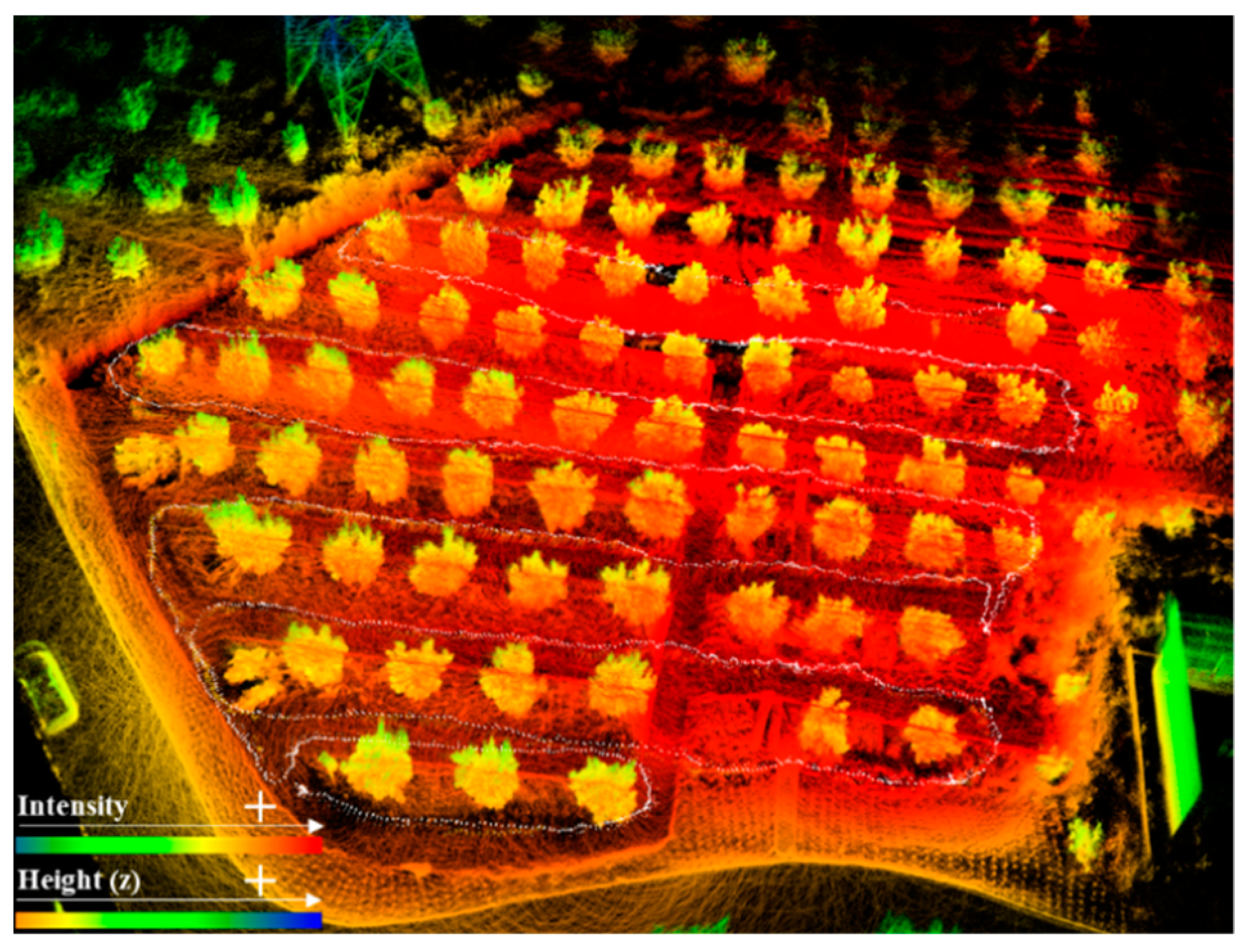
The hand-held 3D LiDAR scanning system consisted of a laser (VLP-16 LiDAR, Velodyne Lidar Co., San Jose, CA, USA), an inertial measurement unit (MTI-30-2A8G4, Xsens Co., Enschede, Holland), and a microcomputer (BRIX GB-BRi7H-8550, GIGABYTE Co., Zhejiang, China). Both are powered by a 12 V Guang Yi Sheng power lithium battery with a capacity of 30 Ah, and the LiDAR system can work continuously for about 6 hours with the power supply. According to the study by Jaakkola et al., the ranging error of a VLP-16 LiDAR scanner is 3 cm, which can meet the needs of forestry applications, and this study used manufacturing values without calibration [45]. The device connection diagram and specific parameters are described in detail in Zhou et al. [46]. The experimenters used a handheld laser radar scanning device to scan the orchard by walking a closed loop path and constructing a 3D map of the orchard (Figure 2).
2.2. Orchard Point Cloud Data Processing
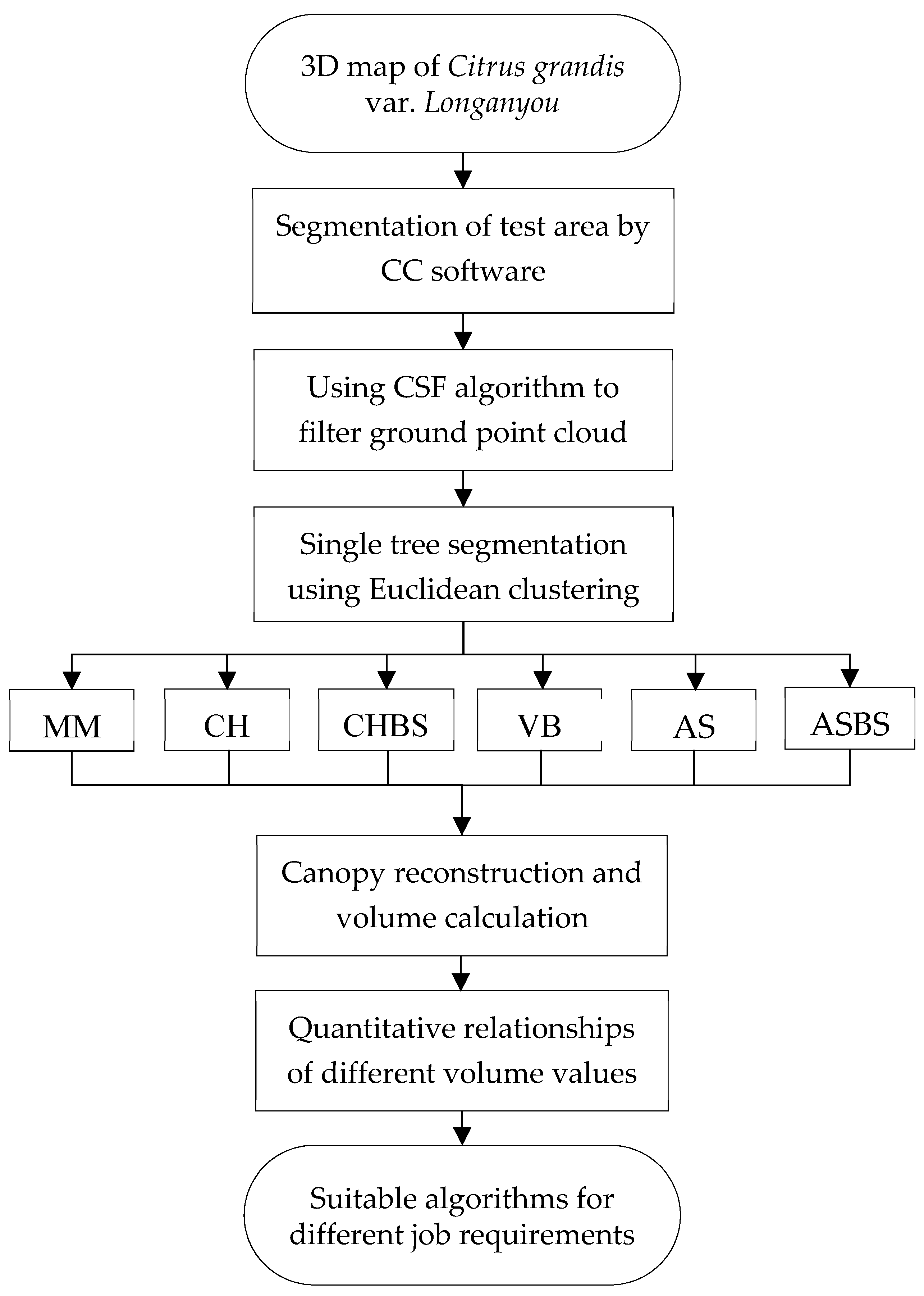
The flow of processing the orchard point cloud data is shown in Figure 3. First, a 3D map of the orchard was constructed using the LiDAR scanning system; next, open-source software, CloudCompare™ (vers. 2.9.1, General Public License software, http://www.cloudcompare.org/, 9 May 2021, CC), was used to segment the test area. To reduce the amount of data processing, the ground point cloud was filtered by the cloth simulation filter (CSF) algorithm [47]. A Euclidean clustering algorithm was then used to segment a single fruit tree, which was convenient for subsequent processing. Each method, MM and APCs (CH, CHBS, VB, AS, and ASBS), was used to realize C. grandis var. Longanyou canopy 3D reconstruction and calculate each tree’s volume. The relationship among the volume values of different algorithms and their adaptation to different scenarios were explored by analyzing different methods of calculation results and the run time.
2.2.1. Ground Filtering
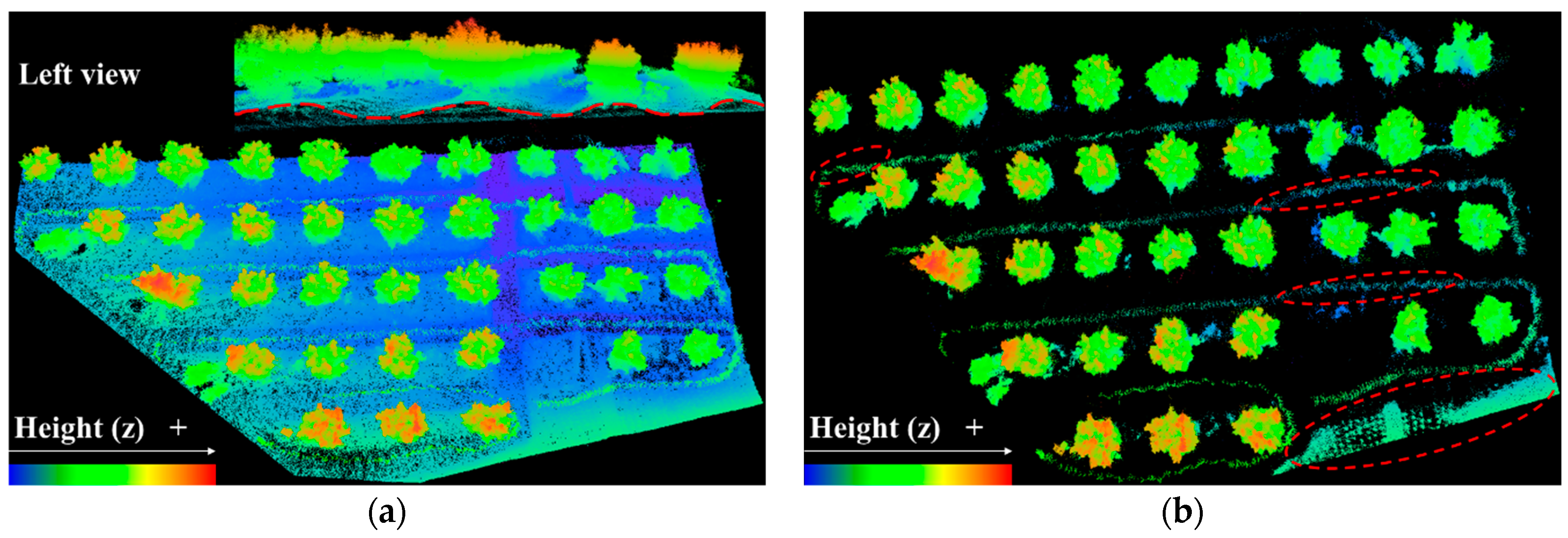
The 3D original point cloud map of the orchard contained both test and non-test areas. CloudCompare™ software was used to select the test area (Figure 4a). To reduce the calculation time for the subsequent processing of point cloud data, the ground point cloud was filtered by appropriate methods based on the ground terrain features. The most commonly used algorithms include the random sample consensus (RANSAC) and CSF algorithms. The RANSAC algorithm is widely used in point cloud plane fitting and segmentation, which is suitable for flat and gentle terrain; the CSF algorithm is suitable for uneven and steep terrain. Because the C. grandis var. Longanyou plantation is located in a hilly area, the ground has an uneven slope; grapefruit is typically grown using the ridge tillage method; the red wavy dotted line in the left part in Figure 4a is a topographic map of the actual ground. Because the terrain undulates, this study used the CSF algorithm to filter the ground point cloud.
The CSF algorithm in CC software has three parameters: Cloth resolution refers to the mesh size of the virtual cloth used to cover the terrain. The smaller the value, the finer the digital terrain model. Max Iterations is the maximum number of iterations of the terrain simulation. The higher this value, the higher the accuracy, but a higher Max Iterations value will require a longer time for calculation. Classification threshold refers to the threshold that divides the point cloud into ground and non-ground parts based on the distance between each point and the simulated terrain. The smaller this value, the smaller the number of ground points filtered out. The three parameter values set in this study were 0.5, 500, and 0.5, respectively. The effect after filtering is shown in Figure 4b. Most of the ground point clouds were filtered out, although there were a few sparsely scattered ground point clouds (inside the red ellipses around dotted lines); this did not affect the extraction of individual fruit trees.
2.2.2. Individual Tree Segmentation
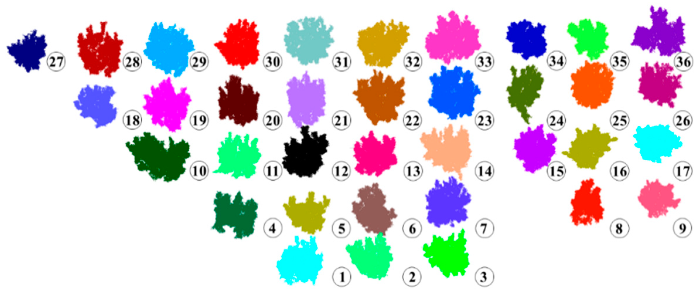
After filtering the ground point clouds in the test area, an appropriate clustering algorithm should be used for point cloud segmentation in combination with crop growth characteristics to obtain a point cloud data of each individual fruit tree. Clustering algorithms based on 3D point clouds mainly include the Density-Based Spatial Clustering of Application with Noise [48], K-means clustering [49], and European clustering [50]. European clustering was used to extract individual fruit trees because the C. grandis var. Longanyou trees had been planted with uniform spacing and had little shade between each other. The method of searching for the nearest neighbor based on the Euclidean distance uses the kd-tree data structure. The decisive parameters in a Euclidean clustering algorithm are MinClusterSize and MaxClusterSize, which are the minimum and maximum number of points in the cluster (or in this case, representing a fruit tree), respectively. The smaller these two values, the more types are included after segmentation. ClusterTolerance refers to the tolerance variable of the distance between the points in the cluster. If the tolerance value is too small, the label marked as one tree can be considered to represent multiple trees. Conversely, if the tolerance value is too large, multiple trees will be marked as a single tree. According to the actual planting tree-row spacing and plant spacing of C. grandis var. Longanyou within each row, the three parameter values in this article were set as 50,000, 5,000,000, and 0.05 m, respectively. The clustering results shown in Figure 5 show each tree represented by a different color. Simultaneously, the European clustering algorithm also removes any residual ground points from the cloud (Figure 4b).
2.3. Calculation of Canopy Height and Crown Width of Fruit Trees
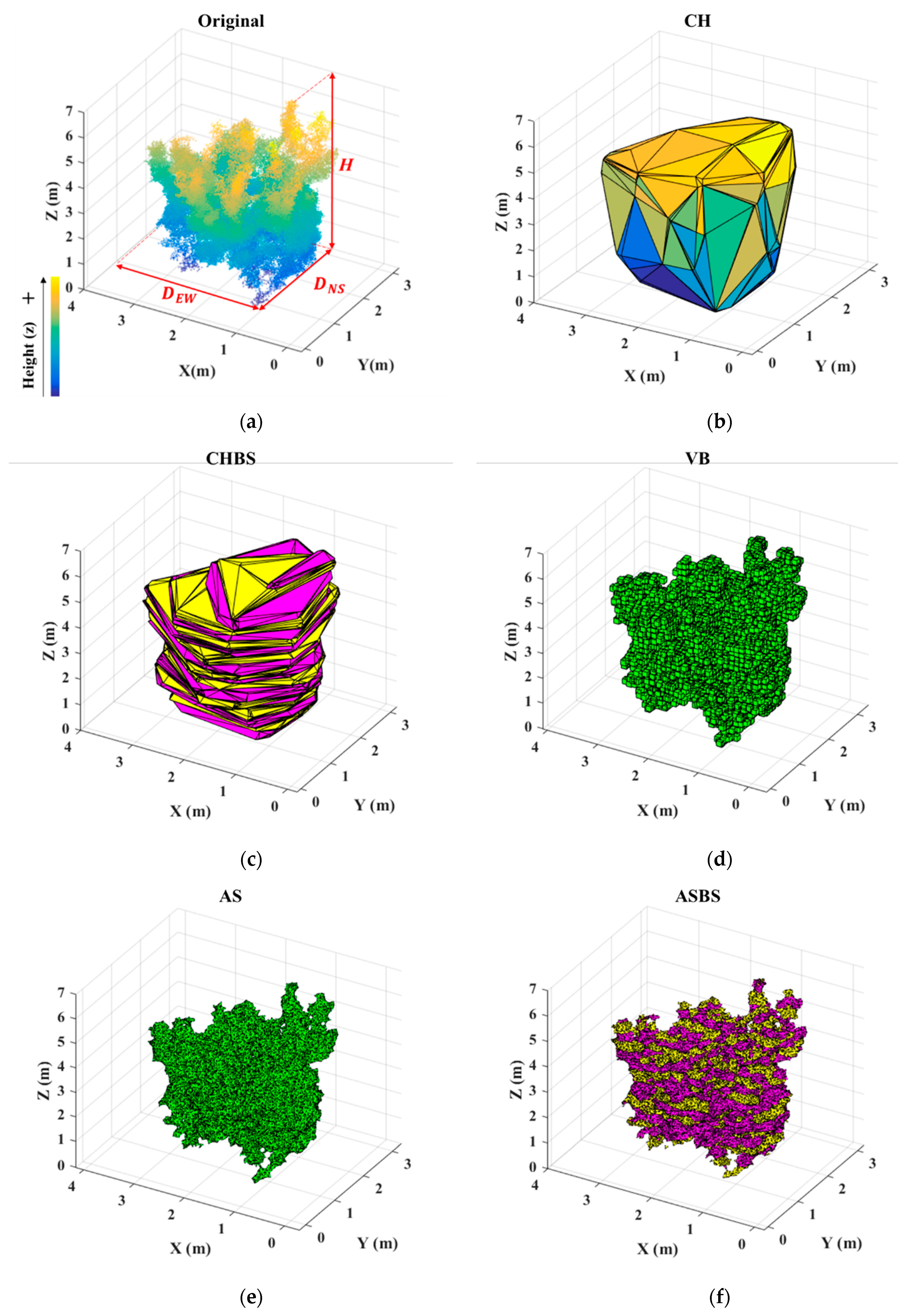
The crown height (H) and crown width (W) of fruit trees are both important characteristic variables of the crown structure (Figure 6), which directly affects the productivity and vitality of fruit trees, and can also reflect the yield of fruit. Obtaining crown height and width is convenient for orchard management, and in some countries managers determine pesticide dose according to crown height [13]. Forest canopy height refers to the distance from the highest point of the canopy to the first live branch above the ground. For C. grandis var. Longanyou, because its tree height is much lower than tree height in natural forests and the branches droop to touch the ground, the crown height of grapefruit was recorded as the distance from the highest point to the lowest point of the fruit tree point cloud according to Yang’s definition [2]. Therefore, crown height was calculated using Equation (1):
where Zmax and Zmin are the maximum and minimum values of Z-axis point cloud, respectively.
Crown width refers to the average north–south and east–west widths of trees, and is usually used to indicate the specifications of trees and fruit tree [51]. This study used Equation (2) to calculate canopy width:
where DNS is the north–south width and DEW is the east–west width.
2.4. Canopy Reconstruction and Volume Calculation
In this study, MM and APCs (CH, CHBS, VB, AS, and ASBS) were used to reconstruct the canopy of fruit trees, with the aim of calculating the canopy volume. All programs of APCs were run in MATLAB 2016A (Mathworks, Natick, MA, USA).
2.4.1. MM Method
Because C. grandis var. Longanyou are a type of citrus tree and because many researchers have often chosen an ellipsoid as the geometric model of a typical citrus tree canopy [14], this study used an ellipsoid model to represent the canopies of C. grandis var. Longanyou trees. The model diagram (Figure 6) used a blue ellipsoid for the fitting geometry of this manual measurement model, and the volume was calculated using Equation (3):
where H and W were measured three times using CC software to calculate the average volume [52].
Figure 7a provides a schematic diagram of canopy measurements.
2.4.2. CH Algorithm
Researchers have used four main methods to calculate tree canopy volume using the convex hull method: incremental, gift wrap, divide and conquer, and the quickhull method. The quickhull method was used in the present study [53]. This algorithm removes any points that are not within the bounds of each closed convex hull (that is, any internal points), and represents each tree crown as a 3D convex polyhedron with a triangular surface (Figure 7b). The volume determined by a CH algorithm contains all of the simplexes belonging to the smallest convex set containing point data.
2.4.3. CHBS Algorithm
The method using a CHBS algorithm mainly segments a point cloud in the Z direction based on a certain number (N) of slices; then, the point cloud is divided into N parts, and the CH algorithm is performed for each segmented point cloud. Finally, the sum of the convex hull volumes of all slices cumulatively is considered the volume of each canopy. Different slice numbers influence the experimental results differently. Because at least three points are required for each slice when calculating the volume with a CH or AS algorithm, Yan initially chose 15 cm spacing in the study of slices [44]. Furthermore, is 3.302 m in this study (Table 1). Therefore, to ensure that the two algorithms cover more points on the slice and facilitate the following comparative analysis, the N value in this study was 20. Figure 7c shows the effect diagram of crown reconstruction using a CHBS algorithm. The influence of different slice numbers on the calculation of canopy volume and operation performance of the CH algorithm is discussed in detail in Section 3.2.5 below.
2.4.4. VB Algorithm
The VB algorithm produces a representation of the point cloud with a small cube having certain specifications; the algorithm counts the number of cubes containing the canopy point cloud. Given the volume of the small cube, the volume of the canopy can be calculated by the number of cubes and the volume of each small cube [39]. For any irregular tree crown, a VB algorithm only needs to consider the size and validity of each cube, without considering the crown shape. Wei [54] considered that the canopy had many gaps rather than being a single entity, and used the VB method to calculate the canopy volume. The results show that the calculated canopy volume tends to be stable when the voxel size is equal to one-tenth of the canopy width. Because in this study is 3.302 m (Table 2), Lecigne [55] confirmed that a smaller voxel size is more suitable for observing subtle changes in spatial exploration than a larger voxel size in the results obtained with simulation data. Based on the specific parameters of C. grandis var. Longanyou, the voxel size of this study was 0.1 m; the VB algorithm effect diagram is shown in Figure 7d.
2.4.5. AS Algorithm
The AS algorithm is a concave hull algorithm. In this method, the simplex of the underlying triangulation is compared with the specified α, deleting the simplex with an empty external sphere and a square radius greater than the defined α. Then the volume of the 3D object is calculated [56]. It should be noted that when α is large enough, the canopy reconstruction effect will be similar to that of a CH algorithm.
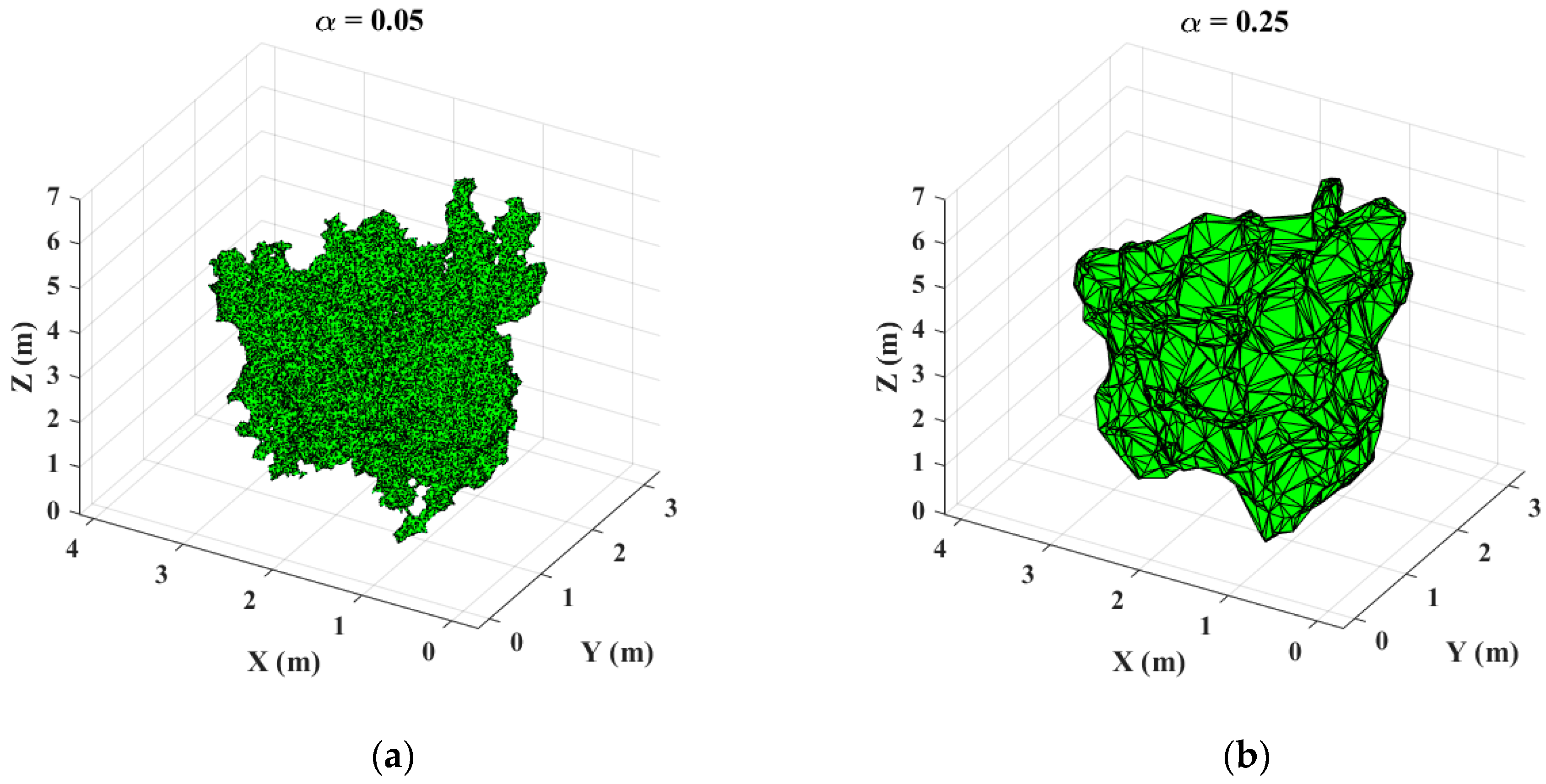
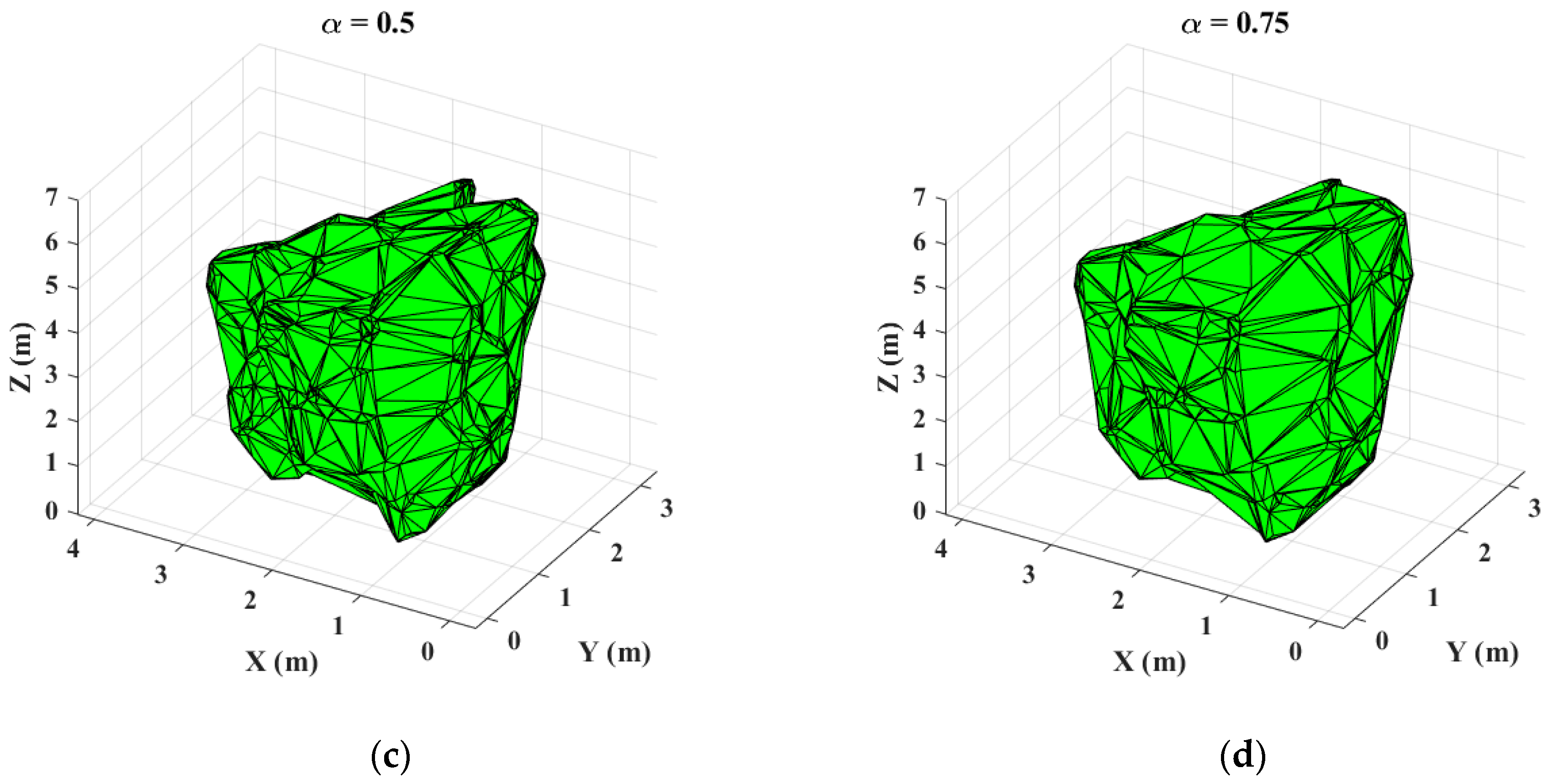
The parameter α is used to determine the level of detail of the obtained triangulation, which in turn controls the fineness of the generated polyhedron, which directly affects the surface reconstruction results [15,57]. Because the slender branches of tree number 1 are more scattered than those of other trees, its crown contour contains a large amount of detailed information, which is more representative than other trees. Figure 8 takes tree number 1 as an example, showing the canopy reconstruction effects under different values for α. When α = 0.05, the canopy structure of fruit trees is expressed in a detailed manner, which expresses the canopy topological structure and degree of density. When α is 0.25 and 0.5, smaller pores in the fruit tree canopy are surrounded by triangles, which only show the spatial extension of the canopy structure, but not the detailed branching characteristics. When α = 0.75, the canopy is completely wrapped, generating a convex hull of the external point cloud, and is unable to express the information in the internal structure. According to the above analysis, by setting different values of α, different models of a fruit tree canopy can be obtained, and different 3D structures can be reconstructed, which can reflect different spatial morphologies, degrees of density, and branching characteristics of the canopy. By comparing the effect diagrams of different values and CH algorithms, it can be clearly found that when α = 0.75 (i.e., far larger than 0.05) the canopy reconstruction diagram is similar to the diagram of the CH algorithm. This phenomenon is also the same as the principle of the two algorithms. In this study, α was selected as 0.05; the effect diagram of the AS algorithm is shown in Figure 7e.
2.4.6. ASBS Algorithm
The principle of the ASBS algorithm is similar to that of the CHBS algorithm. The only difference is that the AS algorithm was used for canopy reconstruction and volume calculation for the sub-parts equally divided along the Z-axis. As with the CHBS algorithm, the value of N was set at 20 in this study; the effect diagram of the ASBS algorithm is shown in Figure 7f. The number of slices in the ASBS algorithm is also discussed in detail in Section 3.2.5 below.
3. Results and Discussion
3.1. Crown Height and Crown Width
The mean, maximum, and minimum, in addition to the variance, absolute error (AE), and relative error (RE) of MM and APCs for the crown height (H) and width (W) of 36 C. grandis var. Longanyou trees are shown in Table 1 and Table 2.
Table 1 and Table 2 show that the RE difference between the MM and APCs results was very small, and the RE of W was even smaller (the RE of H was 0.054, and the RE of W was 0.031). This indicates that the collected point cloud data are similar to the actual data, and the method used can replace the MM to a certain extent, providing a more accurate data basis and a reliable method for the calculation of canopy volume below.
3.2. Crown Volume
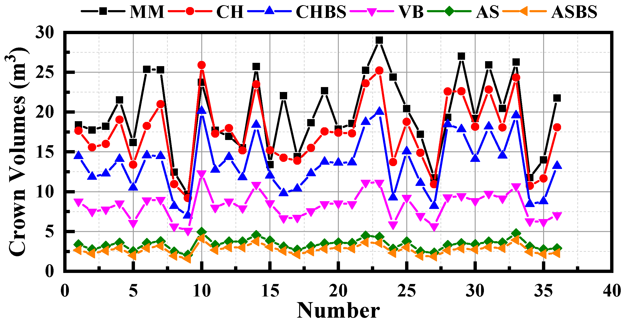
The canopy volumes of 36 C. grandis var. Longanyou trees were calculated using MM and five different APCs (Figure 9). The purpose of this step was not to verify the volume estimation, but to compare different canopy reconstruction methods, combined with the algorithm principle, to understand the differences resulting from different algorithms applied to the canopy of C. grandis var. Longanyou. Then the quantitative relationships of volume values among different algorithms, and the selection of appropriate algorithms for different operation requirements, is discussed.
3.2.1. Comparative Analysis of Six Different Methods
The relationship of measured volumes for a single plant was VMM > VCH > VCHBS > VVB > VAS > VASBS (Figure 9). Among these, the calculated canopy volumes from the MM model were greater than those of all canopy volume calculations by APCs ( = 19.60 m3); VVB was about half of VCH ( = 17.45 m3, = 8.25 m3); VASBS was about one-third of VVB ( = 2.74 m3). The significant differences and algorithm characteristics of these calculation results are closely related to the structural characteristics of the canopy of a C. grandis var. Longanyou tree.
MM treats the tree crown as an ellipsoid and then the canopy volume can be calculated. In addition to the internal holes in an actual canopy, this method also includes the external space between the canopy and the theoretical model (Figure 6). Of particular note, it appears that there are fewer internal holes and gaps in Figure 6 because the canopy of C. grandis var. Longanyou is only seen from one angle. In fact, the internal holes and gaps in the canopy are much larger than those shown in the figure. Therefore, the volume value calculated by MM method is much larger than the real volume of the canopy. The CH algorithm establishes a minimum convex hull based on the canopy point cloud as a whole (Figure 7b), and holes and gaps between branches and leaves are regarded as part of the canopy; this method also creates a larger calculated volume than the actual volume of the canopy. The CHBS algorithm divides the entire canopy into several sub-parts, and establishes the sub-part of the convex hull with partial point clouds as the calculation object; however, the algorithm still contains many holes and gaps, and the calculated volume is still larger than the actual volume of the canopy. Because the VB algorithm treats the point cloud of branches and leaves as a carrier to build small cubes, the internal holes hidden by external branches and leaves can be removed when using this algorithm; as a result, the calculated volume is greatly reduced. However, because 3D cubes are formed, the final volume will be larger than the result of an AS-related algorithm. The AS algorithm can form a smaller envelope network with a reasonable setting of α, and most holes and gaps are consequently removed to form the actual contours of the canopy. Therefore, VAS is smaller and VASBS is minimized.
The mean and variance of canopy volume calculated by MM are the largest, whereas those calculated by the ASBS algorithm are the smallest. In addition, the variance of the six methods decreases and tends to be stable as the volume decreases, which indicates that the holes and gaps between branches and leaves are the main factors affecting the canopy volume.
The volumes calculated by the six methods were fitted for analysis to explore the relationships between the different methods (Table 3). The R2 of MM and APCs were relatively small, between 0.432 and 0.699. The R2 between the five canopy-reconstruction and volume-calculation algorithms based on point clouds were between 0.719 and 0.996. The regression coefficients of each algorithm in Table 3 are consistent with the numerical relationships in Figure 9. Next, a comparative analysis among the APCs used here is described in detail.
3.2.2. Comparison between the MM and APCs
The regression coefficients of VMM and VCH are close to 1, indicating that the two values are very close, but their R2 is small (only 0.699). The is because an ellipsoid entity was used to simulate the canopy volume, which contains not only the holes and gaps inside the canopy, but also includes a small amount of space outside each canopy, resulting in excessive results and a large error in the estimation of canopy volume [18]. The increasing regression coefficient of VMM and other volume measurements means that the difference between VMM and other values increases, and the R2 of linear fitting between VMM and other volume measurements decreases with an increase in the difference in volume. This occurs because the ellipsoid model and CH algorithm overestimates the canopy volume compared with the actual value, and the canopy contains a large number of holes, whereas the VB and AS-related algorithms reduce a larger number of holes, and therefore the difference between the calculated volume of MM and APCs steadily increases, which leads to the above-mentioned trend of the regression coefficient and R2. When Li et al. [18] studied the volume of the canopy of citrus trees, they found that the envelope volume measured by the most external branches and leaves of the canopy was measured by MM, whereas the canopy volume calculated accurately by APCs through the spatial distribution of branches and leaves was closer to the actual volume. Therefore, the canopy volume calculated by APCs was generally smaller than VMM, which is consistent with our research results.
In summary, the MM model requires measures of the parameters for each tree individual and the selection of an appropriate geometry model. The differences in tree canopies make it difficult to have a unified geometric model suitable for replacing the actual canopy shape, and external space will exist between any geometric model and the real shape of the canopy, which will be much larger than the real volume of the canopy. Therefore, the calculated MM volume is far less accurate than those found using the five APCs.
3.2.3. Comparison of Canopy Volume Measured by APCs
Although VVB is approximately 47.3% and 61.1% of VCH and VCHBS, respectively, the R2 values are 0.898 and 0.920, respectively. The essence of the CH-related algorithm is to create an entity surrounded by triangles whose vertex is the outermost point of the point cloud data obtained by LiDAR. This volume includes all of the internal holes and the outer space between the branches and leaves; as a result, it overestimates the apparent volume. Even if the CHBS algorithm is used, the holes between the slices can be eliminated, but not effectively removed. In the VB algorithm, when no point cloud exists in these cubes, the voxels are not considered when calculating the total volume, which is why VCHBS is larger than VVB.
In the present study, VAS and VASBS were approximately 41.1% and 33.2% of VVB, respectively, and the R2 values were 0.876 and 0.874 when comparing VVB to VAS or VASBS, respectively. Because the AS algorithm forms 3D models of all point clouds surrounding the canopy from the outside to the inside, each vertex is composed of point clouds, whereas the VB algorithm has a fixed-size voxel formed with the point cloud as the center. Therefore, the spatial volume of the voxelized 3D canopy model is larger than the polyhedron formed by the AS algorithm. As VASBS becomes smaller, the above volume relationship exists and R2 decreases slightly (from 0.875 to 0.874).
The volume of the CH-related algorithm was much higher than that of the AS-related algorithm, and the regression coefficient between them was approximately 5; R2 was around 0.72. Although both the CH and AS algorithms use a 3D model to form the canopy from the outside to the inside, the CH algorithm uses a simplex of minimum convex triangulation, whereas the AS algorithm is a concave shell algorithm that uses the parameter α to limit the number of simple bodies in the triangulation to obtain more detailed shapes [15]. Therefore, when forming the envelope network on the surface of the canopy, the AS algorithm can effectively remove the holes and gaps inside the canopy, forming a more appropriate 3D model that is more consistent with the actual shape of the canopy. Based on the above discussion, the regression coefficients of the CH-related and AS algorithms are far larger than 1. In addition, because VASBS is the smallest with the addition of slices, the regression coefficient of the CH and ASBS algorithms (6.392) is greater than that between the CH and AS algorithm (5.492).
3.2.4. Running Time Analysis of APCs
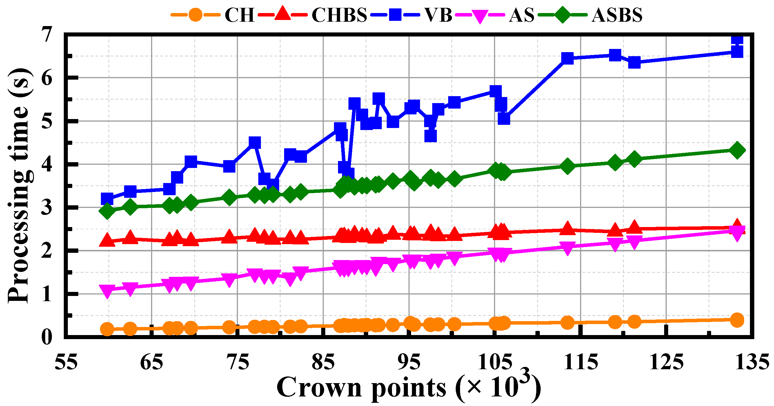
Five APC programs were run in MATLAB 2016a software on a Lenovo computer (processor Intel Core™ i7-8550U @1.80 GHz, 16 GB DDR4 2666 MHz memory, 256 GB SSD), and all other applications were shut down while running the program. To better compare and analyze these five algorithms, the run times of different algorithms were also calculated (Figure 10).
Figure 10 clearly shows the relationships between the run times for the five algorithms. These run times were = 0.277, = 1.699, = 2.343, = 3.909, = 4.867. Because CH and AS algorithms essentially form a 2D plane successively, whereas the VB algorithm forms a 3D voxel, the run time of the VB algorithm was the longest. The order of stability from strong to weak was CH, CHBS, AS, ASBS, VB. Because the number of point clouds in each tree was different, the number of small cubes generated by voxel was significantly different for point clouds with different structures, whereas the differences in 2D planes generated by the CH and AS algorithms were very small. Therefore, the stability of the VB algorithm was minimal; specifically, the variance was the largest (0.974). The slice variance increases because the point cloud distribution of different layers varied and the run time for forming the plane was disparate.
Based on the reconstruction effect, volume, and run time, the MM volumes were far higher than the actual volumes of the canopies; this method is time-consuming and laborious, making it inferior to the developed algorithms based on point clouds. The CH algorithm overestimates the actual canopy volume, but its run time is the shortest ( = 0.277s), and therefore it can be used for real-time obstacle avoidance by agricultural robots in an orchard [58]. The VB algorithm can better reflect the 3D spatial state of the canopy. The value of VVB falls within the mid-range for volume measurement, but it also required the longest run time ( = 4.867s) which fluctuated greatly. Therefore, the VB algorithm could be selected to calculate canopy volume off-line, and to precisely measure relevant parameters of leaves, such as leaf area and LAD [39,59]. The AS algorithm can better express the actual shape of the actual canopy. The VAS measurement was comparatively small, allowed more accurate reconstruction of the true shape of the canopy, and the run time of VAS was in the mid-range among the five processing times; as a result, VAS can be used to evaluate biomass and identify tree species. The slice-related problem is described below.
3.2.5. Discussion on the Different Number of Slices Used with CH and AS Algorithms
Different numbers of slices will produce different results for the reconstruction efforts and result in different volumes of the same C. grandis var. Longanyou canopy; furthermore, the number of slices will also affect the run time of algorithms. The slice spacing was selected as 10 and 5 cm by Fernández-Sarría and Bi, respectively [41,42]; the of C. grandis var. Longanyou was 3.302 m combined with the above. Therefore, five different slice numbers (N = 10, 20, 30, 40, 50) were selected to discuss the influence of different numbers of slices on CH and AS algorithms from the two perspectives of calculated volume and run time.
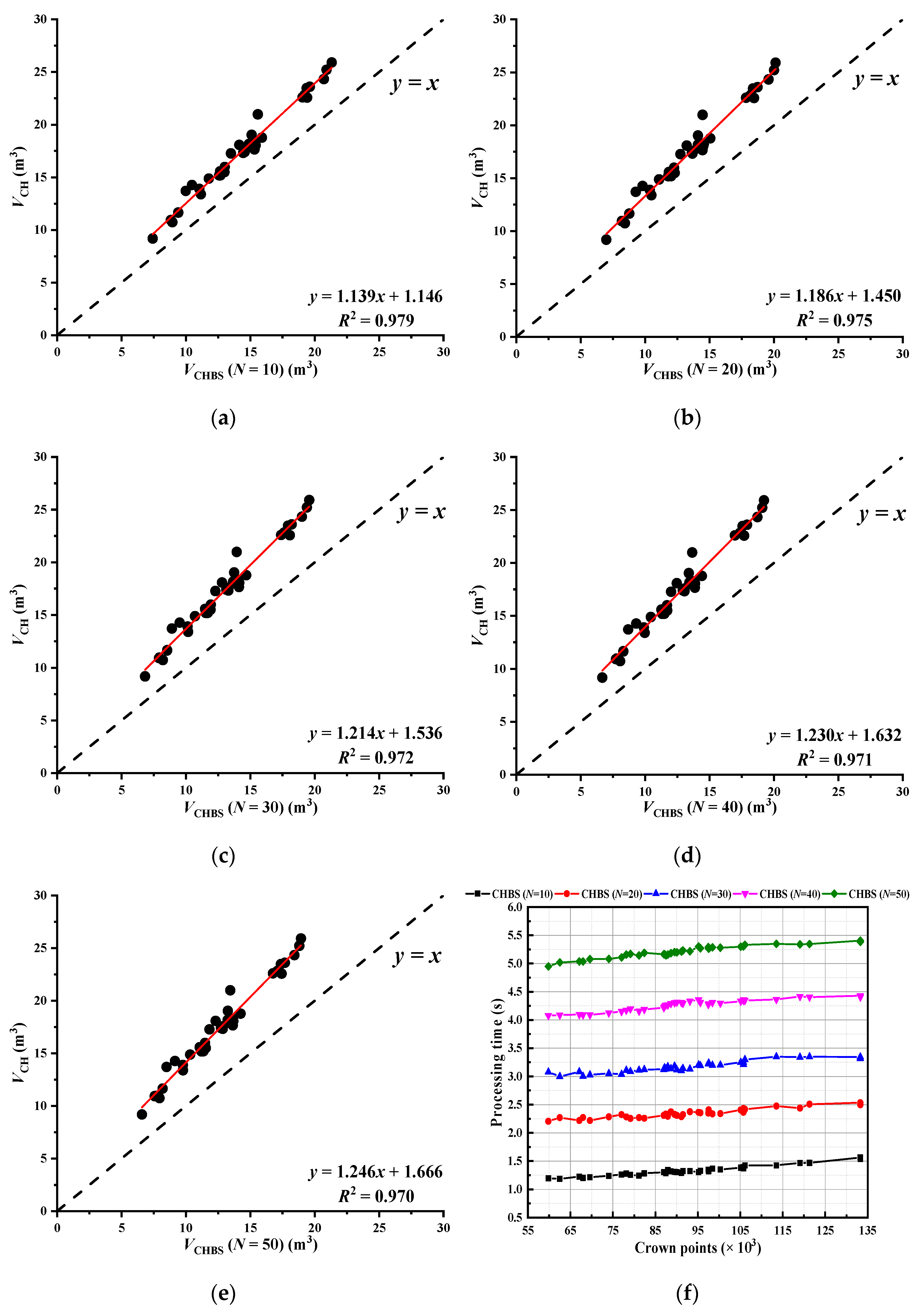
Based on the original CH algorithm, the percentages of holes and gaps removed by different number of slices (N = 10, 20, 30, 40, 50) were 12.2%, 15.7%, 17.6%, 18.7%, 19.7% respectively. As shown in Figure 11a–e, VCHBS decreased with an increasing N; the difference between VCH and VCHBS increased slightly, which resulted in the regression coefficient gradually moving away from 1, and R2 decreased to a small extent. According to the above, this occurred because the method of slicing divides the total crown volume into a certain number of sub-polyhedrons along the Z-axis, removing some holes and gaps in the volume calculated by the CH algorithm. As N increased, more holes and gaps were removed so that the difference in the volume increased and the actual crown shape at each height was better approximated.
In terms of run time, the corresponding run time will increase by 1 s for each increase of ten slices. However, the volume estimated by the CHBS algorithm decreased as the increase in the number of point clouds was small, and the difference between the minimum and maximum run times for the same number of slices was no more than 0.5 s (Figure 11f). This indicates that the operation time of the CHBS algorithm was stable with a different number of point clouds.
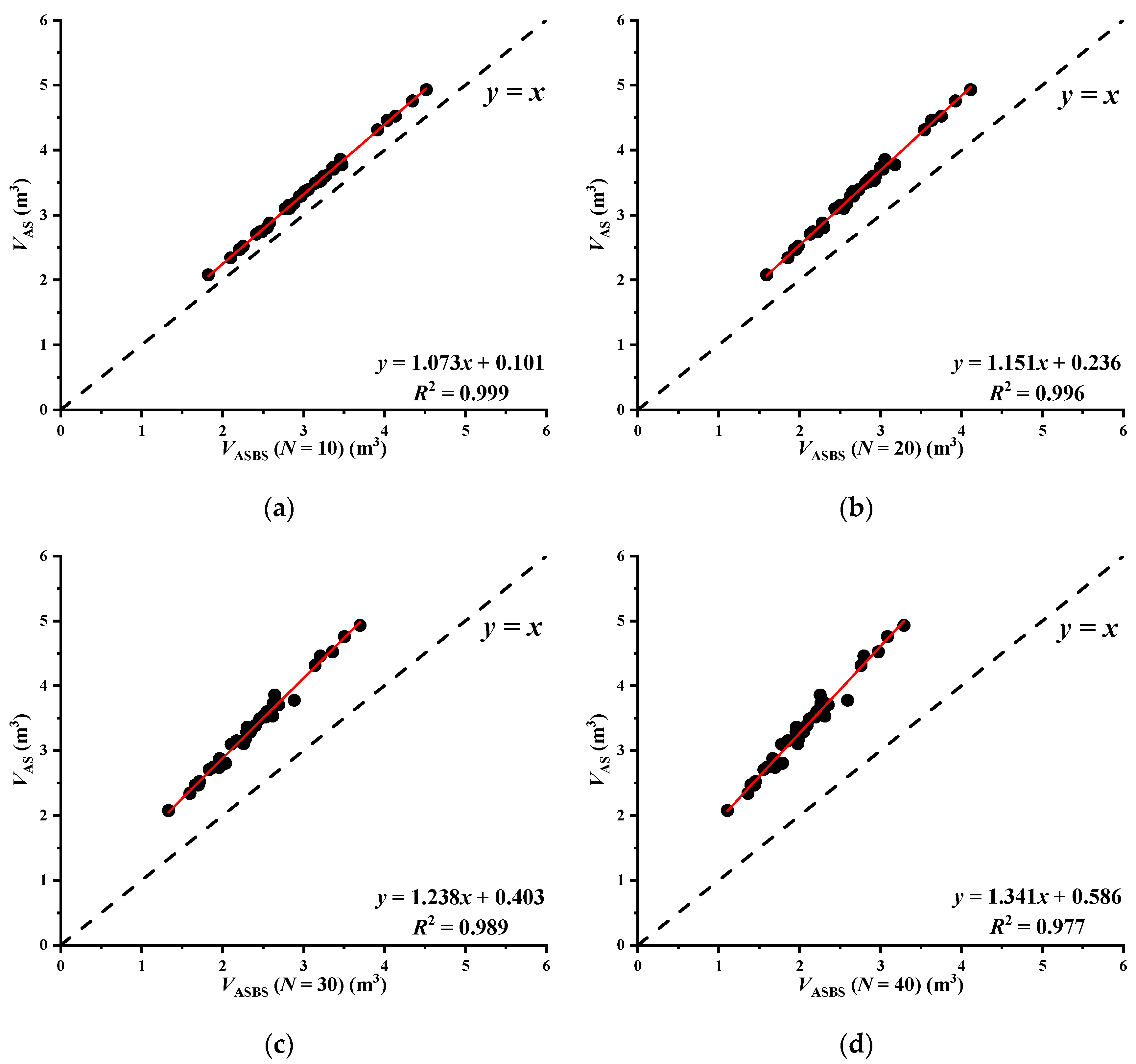
On the basis of the original AS algorithm, the percentages of holes and gaps removed by different number of slices (N = 10, 20, 30, 40, 50) were 6.8%, 13.1%, 19.2%, 25.4%, 32.0% respectively. The relationships, trends, and causes of the differences between the VAS and VASBS measurements were similar to those for VCH and VCHBS, and will not be repeated here (Figure 12a–e). Note that when the number of slices was small (N = 10, 20, 30), the R2 between AS and ASBS algorithms was greater than that between CH and CHBS algorithms (R2 of AS and ASBS was above 0.98, and the maximum R2 of CH and CHBS was 0.979). The R2 of AS and ASBS decreased with the increase in the slice number, and the attenuation was greater than that of CH and CHBS. In addition, the regression coefficient of AS and ASBS increased with an increase in the number of slices, and the amplification was greater than that of CH and CHBS. This shows that the AS algorithm can better remove the holes and gaps in the tree canopy than the CH algorithm, which is the same as the results presented based on the principles of these two algorithms.
In terms of run time, TASBS was 1 s longer than TCHBS for the same number of slices. When the number of slices increased by ten slices, the run time of TASBS also increased by 1 s, and its value significantly increased. The difference between the minimum and maximum run times for the same number of slices was about 1 s (Figure 12f). This shows that the ASBS algorithm had a large range of fluctuation in run times under different numbers of point clouds.
In summary, for the canopy of C. grandis var. Longanyou, adding different slices to the CH algorithm will affect its operating efficiency. The R2 values between VCH and different VCHBS values were 0.970–0.979, which means that the VCH can be calculated, and the different VCHBS also can be calculated using a linear fitting model. As the N increased in CHBS, fewer holes and gaps were removed, but the time was increased. Therefore, the CHBS algorithm is not suitable to calculate the canopy volume of C. grandis var. Longanyou. On the contrary, with the increase in N in ASBS, a greater number of holes and gaps were removed. Although the time was also increased, the R2 values between AS and different VASBS were 0.962–0.999, and different VASBS values were also able to be calculated by VAS. In addition, according to the above fitting relationship of the volumes calculated by different algorithms, the R2 of VCH and VVB was 0.898, and the R2 of VVB and VAS was 0.876. Therefore, VVB can be calculated by VCH, and VAS can then be obtained. Combined with the above analysis of slices, it can be seen that VASBS can be further obtained based on the obtained VAS. In addition, the above conclusion shows that the run time of the CH algorithm was the shortest ( = 0.277). Therefore, for the canopy of C. grandis var. Longanyou, the CH algorithm with the shortest time can be used to obtain the accuracy of the AS algorithm, and even the higher accuracy of the ASBS algorithm, which provides a better approximation of the actual shape of fruit tree canopy.
4. Conclusions
The canopy reconstruction and volume calculation of Citrus. grandis var. Longanyou were realized by the MM and five APC algorithms in this article. The specific research contents are summarized as follows:
- (1)
- A set of processing procedures is available for the extraction of point cloud parameters of the fruit tree canopies specifically for the ridge-tillage planting characteristics of C. grandis var. Longanyou in hilly and mountainous areas, forming a theoretical system for canopy volume analysis of this species. In addition, compared with five APC algorithms, it is difficult to select an appropriate geometric MM model, and the MM method takes a large amount of time, making it inefficient. Therefore, the APC algorithms were proven to be convenient and reliable for the calculation of canopy volume.
- (2)
- A suitable algorithm can be selected based on the different operational needs of C. grandis var. Longanyou: the CH algorithm is suitable for real-time obstacle avoidance and path planning for agricultural robots in orchards; LAI, LAD, and other leaf-related parameters in an offline state can be calculated by the VB algorithm; and the AS algorithm can be used for biomass estimation, tree species identification, and other operations in orchards. Furthermore, the AS algorithm was optimized by slicing in this study, and results of the ASBS algorithm were closer to the actual canopy shape. Although the running times were higher, the R2 values of the pairs of CH and VB, VB and AS, and AS and ASBS were all above 0.85, indicating good linear quantitative relationships existed among different volume values. Therefore, the high-precision volume value (VASBS) can be calculated via the quantitative relationships using the CH algorithm, with the shortest running time.
- (3)
- Changing the number of slices had little influence on the volume calculated using the CH algorithm, but had a significant influence on the AS algorithm results. Furthermore, the addition of slices affected the running efficiency of the algorithm. Therefore, for the calculation of C. grandis var. Longanyou canopy volume, the CH algorithm cannot be optimized with adding slices. By comparison, the implementation of slicing optimization with the AS algorithm is dependent on specific conditions. In addition, because R2 values between CH and different CHBS, AS, and different ASBS algorithms were greater than 0.95, the different volumes determined using the CHBS and ASBS algorithms under different slices can be calculated using only the CH and AS algorithms.
Discrete surfaces will be formed when α is set to a value that is too small, resulting in incomplete reconstruction results. Consequently, the effective implementation of the ASBS algorithm results in significant relationships with the distribution of the point cloud and the dynamic matching of the values of α and N. This will continue to be explored in depth in future work.
Author Contributions
Conceptualization, Y.W., F.K. and X.L.; methodology, Y.W., F.K. and X.L.; software, X.L. and Y.Y.; formal analysis, F.K. and X.L.; investigation, Y.W. and F.K.; resources, Y.W., F.K. and Y.Z.; data curation, X.L. and Y.Y.; writing—original draft preparation, F.K. and X.L.; writing—review and editing, F.K. and X.L.; supervision, Y.W., F.K. and Y.Z.; project administration, Y.W., F.K. and Y.Z.; funding acquisition, Y.W., F.K. and Y.Z. All authors have read and agreed to the published version of the manuscript.
Funding
This research was funded by the Fundamental Research Funds for the Central Universities (No. BLX201820).
Acknowledgments
We thank LetPub for its linguistic assistance during the preparation of this manuscript.
Conflicts of Interest
The authors declare no conflict of interest.
References
- Zhang, K.P.; Li, R.F.; Liu, S.Y.; He, Q.; Liang, G.L.; Lu, Z.M.; Yi, Y.W.; Hu, T.; Guo, Q.G. Analysis of the Canopy Structural Characteristics of Different Training Systems for Citrus Grandis Var. Longanyou. Acta Ecol. Sin. 2017, 37, 8456–8466. [Google Scholar]
- Yang, H.; Wang, X.; Sun, G. Three-Dimensional Morphological Measurement Method for a Fruit Tree Canopy Based on Kinect Sensor Self-Calibration. Agronomy 2019, 9, 741. [Google Scholar] [CrossRef] [Green Version]
- Jiang, Y.; Li, C.; Takeda, F.; Kramer, E.A.; Ashrafi, H.; Hunter, J. 3D Point Cloud Data to Quantitatively Characterize Size and Shape of Shrub Crops. Hortic. Res. 2019, 6, 1–17. [Google Scholar] [CrossRef] [Green Version]
- Fernández-Sarría, A.; López-Cortés, I.; Estornell, J.; Velázquez-Martí, B.; Salazar, D. Estimating Residual Biomass of Olive Tree Crops Using Terrestrial Laser Scanning. Int. J. Appl. Earth Obs. Geoinf. 2019, 75, 163–170. [Google Scholar] [CrossRef]
- Meng, Y.; Dong, X.; Liu, W.; Lin, W. Modeling Biomass of White Birch (Betula Platyphylla) in the Lesser Khingan Range of China Based on Terrestrial 3D Laser Scanning System. Nat. Resour. Model. 2020, 33, e12240. [Google Scholar] [CrossRef]
- Mészáros, M.; Laňar, L.; Sus, J.; Náměstek, J. Comparison of Two Training Methods Applied to Apple Trees Trained to Slender Spindle During the First Years After Planting. Acta Univ. Agric. Silvic. Mendel. Brun. 2017, 65, 1241–1245. [Google Scholar] [CrossRef] [Green Version]
- Sola-Guirado, R.R.; Castillo-Ruiz, F.J.; Jiménez-Jiménez, F.; Blanco-Roldan, G.L.; Castro-Garcia, S.; Gil-Ribes, J.A. Olive Actual “on Year” Yield Forecast Tool Based on the Tree Canopy Geometry Using UAS Imagery. Sensors 2017, 17, 1743. [Google Scholar] [CrossRef] [Green Version]
- Zhang, X.; Bao, Y.; Wang, D.; Xin, X.; Ding, L.; Xu, D.; Hou, L.; Shen, J. Using UAV LiDAR to Extract Vegetation Parameters of Inner Mongolian Grassland. Remote Sens. 2021, 13, 656. [Google Scholar] [CrossRef]
- Savian, F.; Martini, M.; Ermacora, P.; Paulus, S.; Mahlein, A.K. Prediction of the Kiwifruit Decline Syndrome in Diseased Orchards by Remote Sensing. Remote Sens. 2020, 12, 2194. [Google Scholar] [CrossRef]
- Hong, S.-W.; Zhao, L.; Zhu, H. CFD Simulation of Pesticide Spray from Air-Assisted Sprayers in an Apple Orchard: Tree Deposition and off-Target Losses. Atmos. Environ. 2018, 175, 109–119. [Google Scholar] [CrossRef]
- Rosell, J.R.; Sanz, R. A Review of Methods and Applications of the Geometric Characterization of Tree Crops in Agricultural Activities. Comput. Electron. Agric. 2012, 81, 124–141. [Google Scholar] [CrossRef] [Green Version]
- Jiang, H.; Liu, L.; Liu, P.; Wang, J.; Zhang, X.; Gao, D. Online Calculation Method of Fruit Trees Canopy Volume for Precision Spray. Trans. Chin. Soc. Agric. Mach. 2019, 50, 120–129. [Google Scholar]
- Martínez-Casasnovas, J.A.; Rufat, J.; Arnó, J.; Arbonés, A.; Sebé, F.; Pascual, M.; Gregorio, E.; Rosell-Polo, J.R. Mobile Terrestrial Laser Scanner Applications in Precision Fruticulture/Horticulture and Tools to Extract Information from Canopy Point Clouds. Precis. Agric. 2017, 18, 111–132. [Google Scholar]
- Schinor, E.H.; Cristofani-Yaly, M.; Bastianel, M.; Machado, M.A. Sunki Mandarin vs Poncirus Trifoliata Hybrids as Rootstocks for Pera Sweet Orange. J. Agric. Sci. 2013, 5, 190. [Google Scholar] [CrossRef]
- Korhonen, L.; Vauhkonen, J.; Virolainen, A.; Hovi, A.; Korpela, I. Estimation of Tree Crown Volume from Airborne Lidar Data Using Computational Geometry. Int. J. Remote Sens. 2013, 34, 7236–7248. [Google Scholar] [CrossRef]
- Miranda-Fuentes, A.; Llorens, J.; Gamarra-Diezma, J.L.; Gil-Ribes, J.A.; Gil, E. Towards an Optimized Method of Olive Tree Crown Volume Measurement. Sensors 2015, 15, 3671–3687. [Google Scholar] [CrossRef] [PubMed] [Green Version]
- da Silva Scapin, M.; Behlau, F.; Scandelai, L.H.M.; Fernandes, R.S.; Junior, G.J.S.; Ramos, H.H. Tree-Row-Volume-Based Sprays of Copper Bactericide for Control of Citrus Canker. Crop Prot. 2015, 77, 119–126. [Google Scholar] [CrossRef]
- Li, P.; Zhang, M.; Wang, T.; Zheng, Y.; Yi, S.; Lee, Q. Real-Time Estimation of Citrus Canopy Volume Based on Laser Scanner and Irregular Triangular Prism Module Method. Sci. Agric. Sin. 2020, 52, 4493–4504. [Google Scholar]
- Zhang, C.; Jiang, Y.; Xu, B.; Li, X.; Zhu, Y.; Lei, L.; Chen, R.; Dong, Z.; Yang, H.; Yang, G. Apple Tree Branch Information Extraction from Terrestrial Laser Scanning and Backpack-LiDAR. Remote Sens. 2020, 12, 3592. [Google Scholar] [CrossRef]
- Ni, Z.; Burks, T.F.; Lee, W.S. 3D Reconstruction of Plant/Tree Canopy Using Monocular and Binocular Vision. J. Imaging 2016, 2, 28. [Google Scholar] [CrossRef]
- Hobart, M.; Pflanz, M.; Weltzien, C.; Schirrmann, M. Growth Height Determination of Tree Walls for Precise Monitoring in Apple Fruit Production Using UAV Photogrammetry. Remote Sens. 2020, 12, 1656. [Google Scholar] [CrossRef]
- Dong, X.; Zhang, Z.; Yu, R.; Tian, Q.; Zhu, X. Extraction of Information about Individual Trees from High-Spatial-Resolution UAV-Acquired Images of an Orchard. Remote Sens. 2020, 12, 133. [Google Scholar] [CrossRef] [Green Version]
- Jurado, J.M.; Ortega, L.; Cubillas, J.J.; Feito, F.R. Multispectral Mapping on 3D Models and Multi-Temporal Monitoring for Individual Characterization of Olive Trees. Remote Sens. 2020, 12, 1106. [Google Scholar] [CrossRef] [Green Version]
- Li, D.; Xu, L.; Tang, X.; Sun, S.; Cai, X.; Zhang, P. 3D Imaging of Greenhouse Plants with an Inexpensive Binocular Stereo Vision System. Remote Sens. 2017, 9, 508. [Google Scholar] [CrossRef] [Green Version]
- Vázquez-Arellano, M.; Reiser, D.; Paraforos, D.S.; Garrido-Izard, M.; Burce, M.E.C.; Griepentrog, H.W. 3-D Reconstruction of Maize Plants Using a Time-of-Flight Camera. Comput. Electron. Agric. 2018, 145, 235–247. [Google Scholar] [CrossRef]
- Zhou, S.; Kang, F.; Li, W.; Kan, J.; Zheng, Y. Point Cloud Registration for Agriculture and Forestry Crops Based on Calibration Balls Using Kinect V2. Int. J. Agric. Biol. Eng. 2020, 13, 198–205. [Google Scholar] [CrossRef]
- Medeiros, H.; Kim, D.; Sun, J.; Seshadri, H.; Akbar, S.A.; Elfiky, N.M.; Park, J. Modeling Dormant Fruit Trees for Agricultural Automation. J. Field Robot. 2017, 34, 1203–1224. [Google Scholar] [CrossRef]
- Qiu, Q.; Sun, N.; Bai, H.; Wang, N.; Fan, Z.; Wang, Y.; Meng, Z.; Li, B.; Cong, Y. Field-Based High-Throughput Phenotyping for Maize Plant Using 3D LiDAR Point Cloud Generated with a “Phenomobile”. Front. Plant Sci. 2019, 10, 554. [Google Scholar] [CrossRef] [Green Version]
- Yun, T.; Jiang, K.; Hou, H.; An, F.; Chen, B.; Jiang, A.; Li, W.; Xue, L. Rubber Tree Crown Segmentation and Property Retrieval Using Ground-Based Mobile LiDAR after Natural Disturbances. Remote Sens. 2019, 11, 903. [Google Scholar] [CrossRef] [Green Version]
- Colaço, A.F.; Trevisan, R.G.; Molin, J.P.; Rosell-Polo, J.R. A Method to Obtain Orange Crop Geometry Information Using a Mobile Terrestrial Laser Scanner and 3D Modeling. Remote Sens. 2017, 9, 763. [Google Scholar] [CrossRef] [Green Version]
- Xiao, S.; Chai, H.; Shao, K.; Shen, M.; Wang, Q.; Wang, R.; Sui, Y.; Ma, Y. Image-Based Dynamic Quantification of Aboveground Structure of Sugar Beet in Field. Remote Sens. 2020, 12, 269. [Google Scholar] [CrossRef] [Green Version]
- Lin, W.; Meng, Y.; Qiu, Z.; Zhang, S.; Wu, J. Measurement and Calculation of Crown Projection Area and Crown Volume of Individual Trees Based on 3D Laser-Scanned Point-Cloud Data. Int. J. Remote Sens. 2017, 38, 1083–1100. [Google Scholar] [CrossRef]
- Vauhkonen, J.; Seppänen, A.; Packalén, P.; Tokola, T. Improving Species-Specific Plot Volume Estimates Based on Airborne Laser Scanning and Image Data Using Alpha Shape Metrics and Balanced Field Data. Remote Sens. Environ. 2012, 124, 534–541. [Google Scholar] [CrossRef]
- Vauhkonen, J.; Næsset, E.; Gobakken, T. Deriving Airborne Laser Scanning Based Computational Canopy Volume for Forest Biomass and Allometry Studies. ISPRS J. Photogramm. Remote Sens. 2014, 96, 57–66. [Google Scholar] [CrossRef]
- Wang, K.; Zhou, J.; Zhang, W.; Zhang, B. Mobile LiDARScanning System Combined WithCanopy Morphology ExtractingMethods for Tree Crown ParametersEvaluation in Orchards. Sensors 2021, 21, 339. [Google Scholar] [CrossRef]
- Yao, W.; Krzystek, P.; Heurich, M. Tree Species Classification and Estimation of Stem Volume and DBH Based on Single Tree Extraction by Exploiting Airborne Full-Waveform LiDAR Data. Remote Sens. Environ. 2012, 123, 368–380. [Google Scholar] [CrossRef]
- Wu, B.; Yu, B.; Yue, W.; Shu, S.; Tan, W.; Hu, C.; Huang, Y.; Wu, J.; Liu, H. A Voxel-Based Method for Automated Identification and Morphological Parameters Estimation of Individual Street Trees from Mobile Laser Scanning Data. Remote Sens. 2013, 5, 584–611. [Google Scholar] [CrossRef] [Green Version]
- Zhang, L.; Li, B.; Zhang, S.; Zhang, L.; Wang, F. Light Interception Measurement of Apple Trees Trained to Tall Spindle Shape Based on Three-dimensional Digitizer. North. Hortic. 2012, 7, 9–12. [Google Scholar]
- Hosoi, F.; Nakai, Y.; Omasa, K. Voxel Tree Modeling for Estimating Leaf Area Density and Woody Material Volume Using 3-D LIDAR Data. ISPRS Ann. Photogramm. Remote Sens. Spat. Inf. Sci. 2013, II-5/W2, 115–120. [Google Scholar] [CrossRef] [Green Version]
- Olsoy, P.J.; Glenn, N.F.; Clark, P.E.; Derryberry, D.R. Aboveground Total and Green Biomass of Dryland Shrub Derived from Terrestrial Laser Scanning. ISPRS J. Photogramm. Remote Sens. 2014, 88, 166–173. [Google Scholar] [CrossRef] [Green Version]
- Fernández-Sarría, A.; Martínez, L.; Velázquez-Martí, B.; Sajdak, M.; Estornell, J.; Recio, J.A. Different Methodologies for Calculating Crown Volumes of Platanus Hispanica Trees Using Terrestrial Laser Scanner and a Comparison with Classical Dendrometric Measurements. Comput. Electron. Agric. 2013, 90, 176–185. [Google Scholar] [CrossRef]
- Bi, Y.; Qi, L.; Chen, S.; Li, L.; Liu, S. Canopy Volume Measurement Method Based on Point Cloud Data. Sci. Technol. Rev. 2013, 31, 31–36. [Google Scholar]
- Cheein, F.A.A.; Guivant, J.; Sanz, R.; Escolà, A.; Yandún, F.; Torres-Torriti, M.; Rosell-Polo, J.R. Real-Time Approaches for Characterization of Fully and Partially Scanned Canopies in Groves. Comput. Electron. Agric. 2015, 118, 361–371. [Google Scholar] [CrossRef] [Green Version]
- Yan, Z.; Liu, R.; Cheng, L.; Zhou, X.; Ruan, X.; Xiao, Y. A Concave Hull Methodology for Calculating the Crown Volume of Individual Trees Based on Vehicle-Borne LiDAR Data. Remote Sens. 2019, 11, 623. [Google Scholar] [CrossRef] [Green Version]
- Jaakkola, A.; Hyyppä, J.; Yu, X.; Kukko, A.; Kaartinen, H.; Liang, X.; Hyyppä, H.; Wang, Y. Autonomous Collection of Forest Field Reference—The Outlook and a First Step with UAV Laser Scanning. Remote Sens. 2017, 9, 785. [Google Scholar] [CrossRef] [Green Version]
- Zhou, S.; Kang, F.; Li, W.; Kan, J.; Zheng, Y.; He, G. Extracting Diameter at Breast Height with a Handheld Mobile LiDAR System in an Outdoor Environment. Sensors 2019, 19, 3212. [Google Scholar] [CrossRef] [Green Version]
- Zhang, W.; Qi, J.; Wan, P.; Wang, H.; Xie, D.; Wang, X.; Yan, G. An Easy-to-Use Airborne LiDAR Data Filtering Method Based on Cloth Simulation. Remote Sens. 2016, 8, 501. [Google Scholar] [CrossRef]
- Wang, X.; Chan, T.O.; Liu, K.; Pan, J.; Luo, M.; Li, W.; Wei, C. A Robust Segmentation Framework for Closely Packed Buildings from Airborne LiDAR Point Clouds. Int. J. Remote Sens. 2020, 41, 5147–5165. [Google Scholar] [CrossRef]
- Hu, C.; Pan, Z.; Zhong, T. Leaf and Wood Separation of Poplar Seedlings Combining Locally Convex Connected Patches and K-Means++ Clustering from Terrestrial Laser Scanning Data. J. Appl. Remote Sens. 2020, 14, 1. [Google Scholar] [CrossRef]
- Gamal, A.; Wibisono, A.; Wicaksono, S.B.; Abyan, M.A.; Hamid, N.; Wisesa, H.A.; Jatmiko, W.; Ardhianto, R. Automatic LIDAR Building Segmentation Based on DGCNN and Euclidean Clustering. J. Big Data 2020, 7, 1–18. [Google Scholar] [CrossRef]
- Gallardo-Salazar, J.L.; Pompa-García, M. Detecting Individual Tree Attributes and Multispectral Indices Using Unmanned Aerial Vehicles: Applications in a Pine Clonal Orchard. Remote Sens. 2020, 12, 4144. [Google Scholar] [CrossRef]
- Colaço, A.F.; Trevisan, R.G.; Molin, J.P.; Rosell Polo, J.R. Orange Tree Canopy Volume Estimation by Manual and LiDAR-Based Methods. Adv. Anim. Biosci. 2017, 8, 477–480. [Google Scholar] [CrossRef] [Green Version]
- Chakraborty, M.; Khot, L.R.; Sankaran, S.; Jacoby, P.W. Evaluation of Mobile 3D Light Detection and Ranging Based Canopy Mapping System for Tree Fruit Crops. Comput. Electron. Agric. 2019, 158, 284–293. [Google Scholar] [CrossRef]
- Wei, X.; Wang, Y.; Zheng, J.; Wang, M.; Feng, Z. Tree Crown Volume Calculation Based on 3-D Laser Scanning Point Clouds Data. Nongye Jixie Xuebao Trans. Chin. Soc. Agric. Mach. 2013, 44, 235–240. [Google Scholar]
- Lecigne, B.; Delagrange, S.; Messier, C. Exploring Trees in Three Dimensions: VoxR, a Novel Voxel-Based R Package Dedicated to Analysing the Complex Arrangement of Tree Crowns. Ann. Bot. 2018, 121, 589–601. [Google Scholar] [CrossRef] [PubMed]
- Hadas, E.; Jozkow, G.; Walicka, A.; Borkowski, A. Determining Geometric Parameters of Agricultural Trees from Laser Scanning Data Obtained with Unmanned Aerial Vehicle. ISPRS Int. Arch. Photogramm. Remote Sens. Spat. Inf. Sci. 2018, XLII–2, 407–410. [Google Scholar] [CrossRef] [Green Version]
- Li, Q.; Gao, X.; Fei, X.; Zhang, H.; Wang, J.; Cui, Y.; Li, B. Construction of Tree Crown Three-dimensional Model Using Alpha-shape Algorithm. Bull. Surv. Mapp. 2018, 12, 91–95. [Google Scholar]
- Cheein, F.A.A.; Guivant, J. SLAM-Based Incremental Convex Hull Processing Approach for Treetop Volume Estimation. Comput. Electron. Agric. 2014, 102, 19–30. [Google Scholar] [CrossRef]
- Wu, D.; Johansen, K.; Phinn, S.; Robson, A. Suitability of Airborne and Terrestrial Laser Scanning for Mapping Tree Crop Structural Metrics for Improved Orchard Management. Remote Sens. 2020, 12, 1647. [Google Scholar] [CrossRef]
Figure 1.
Photos of the test location and scenario: (a) aerial view of the grapefruit orchard; (b) ground-based view of the Citrus grandis var. Longanyou orchard.
Figure 1.
Photos of the test location and scenario: (a) aerial view of the grapefruit orchard; (b) ground-based view of the Citrus grandis var. Longanyou orchard.

Figure 2.
A 3D LiDAR-based map of the Citrus grandis var. Longanyou orchard, colored to indicate reflection intensity and elevation; the white dotted line is the motion trajectory of the LiDAR scanning device.
Figure 2.
A 3D LiDAR-based map of the Citrus grandis var. Longanyou orchard, colored to indicate reflection intensity and elevation; the white dotted line is the motion trajectory of the LiDAR scanning device.

Figure 3.
Data processing flow of 3D point cloud in Citrus grandis var. Longanyou orchard. Note: CC, CloudCompare™ software; CSF, cloth simulation filter (CSF) algorithm; manual method, MM; the canopy reconstruction algorithms based on point cloud: convex hull, CH; convex hull by slices, CHBS; voxel-based, VB; alpha-shape, AS; alpha-shape by slices, ASBS.

Figure 4.
Three-dimensional point cloud maps: (a) initial test area diagram; an inset diagram shows a view looking down orchard rows and to the left, where the red wavy dotted line indicates the topography of the Citrus grandis var. Longanyou orchard; (b) test area diagram after ground filtering, where some ground point clouds still existed in the red dashed ellipse after filtering.

Figure 5.
Clustering results for the experimental area, where each color represents one tree.

Figure 6.
Schematic diagram of manual measurement parameters of Citrus grandis var. Longanyou, where the blue curves show the ellipsoid model, the voids between the canopy and the theoretical model represent external space, and the red parts refer to the parts of the internal holes and gaps between branches and leaves.

Figure 7.
Canopy reconstruction renderings of tree No. 1 with (a) the manual method (MM) and five algorithms based on point clouds: (b) convex hull (CH); (c) convex hull by slices (CHBS); (d) voxel-based (VB); (e) alpha-shape (AS); and (f) alpha-shape by slices (ASBS) algorithms. Note: X, Y, and Z are the three dimensions of the canopy, length, width, and height, respectively.

Figure 8.
Diagrams showing canopy reconstruction of tree No. 1 with different α values: (a) α = 0.05; (b) 0.25; (c) 0.5; (d) 0.75. Note: X, Y, and Z are the three dimensions of the canopy, length, width, and height, respectively.
Figure 8.
Diagrams showing canopy reconstruction of tree No. 1 with different α values: (a) α = 0.05; (b) 0.25; (c) 0.5; (d) 0.75. Note: X, Y, and Z are the three dimensions of the canopy, length, width, and height, respectively.


Figure 9.
The volume values of 36 trees calculated by six methods, indicated by different colors (lesser to greater sequences). Note: manual method, MM; canopy reconstruction algorithms, convex hull, CH; convex hull by slices, CHBS; voxel-based, VB; alpha-shape, AS; alpha-shape by slices, ASBS.
Figure 9.
The volume values of 36 trees calculated by six methods, indicated by different colors (lesser to greater sequences). Note: manual method, MM; canopy reconstruction algorithms, convex hull, CH; convex hull by slices, CHBS; voxel-based, VB; alpha-shape, AS; alpha-shape by slices, ASBS.

Figure 10.
Run time of reconstruction algorithms based on point clouds for crown reconstruction and volume calculation, indicated in order of number of crown points. Canopy reconstruction algorithms included convex hull, CH; convex hull by slices, CHBS; voxel-based, VB; alpha-shape, AS; alpha-shape by slices, ASBS.

Figure 11.
Scatter plot and linear fitting of crown volumes between the convex hull (CH) algorithm and different numbers of slices (N): (a) N = 10; (b) 20; (c) 30; (d) 40; (e) 50. (f) Processing time of different slices using the convex hull by slices (CHBS) algorithm.
Figure 11.
Scatter plot and linear fitting of crown volumes between the convex hull (CH) algorithm and different numbers of slices (N): (a) N = 10; (b) 20; (c) 30; (d) 40; (e) 50. (f) Processing time of different slices using the convex hull by slices (CHBS) algorithm.

Figure 12.
Scatter plot and linear fitting of crown volumes between the alpha-shape (AS) algorithm and different numbers of slices (N): (a) N = 10; (b) 20; (c) 30; (d) 40; (e) 50. (f) Processing time of different slices using the alpha-shape by slices (ASBS) algorithm.
Figure 12.
Scatter plot and linear fitting of crown volumes between the alpha-shape (AS) algorithm and different numbers of slices (N): (a) N = 10; (b) 20; (c) 30; (d) 40; (e) 50. (f) Processing time of different slices using the alpha-shape by slices (ASBS) algorithm.


Table 1.
Comparative analysis of crown height obtained using MM and APCs.
| H | Manual (m) | Algorithm (m) | Absolute Error (m) | Relative Error |
|---|---|---|---|---|
| Mean | 3.302 | 3.432 | 0.167 | 0.054 |
| Var. | 0.146 | 0.099 | 0.019 | 0.002 |
| Max | 4.080 | 4.262 | 0.575 | 0.255 |
| Min | 2.250 | 2.825 | 0.002 | 0.001 |
Table 2.
Comparative analysis of crown diameters obtained using MM and APCs.
| W | Manual (m) | Algorithm (m) | Absolute Error (m) | Relative Error |
|---|---|---|---|---|
| Mean | 3.336 | 3.348 | 0.105 | 0.031 |
| Var. | 0.088 | 0.114 | 0.021 | 0.001 |
| Max | 3.825 | 4.340 | 0.769 | 0.215 |
| Min | 2.729 | 2.837 | 0.004 | 0.001 |
Table 3.
Equations relating crown volumes calculated by six different methods and R2.
| Equation/R2 | VMM | VCH | VCHBS | VVB | VAS | VASBS |
|---|---|---|---|---|---|---|
| VMM | y = 0.954x + 2.965 | y = 1.076x + 5.083 | y = 2.069x + 2.544 | y = 4.891x + 3.027 | y = 5.864x + 3.536 | |
| VCH | 0.699 | y = 1.186x + 1.449 | y = 2.382x − 2.196 | y = 5.492x − 1.163 | y = 6.392x − 0.066 | |
| VCHBS | 0.614 | 0.975 | y = 2.008x − 3.066 | y = 4.586x − 2.045 | y = 5.295x − 1.013 | |
| VVB | 0.515 | 0.898 | 0.920 | y = 2.410x + 0.090 | y = 2.773x + 0.649 | |
| VAS | 0.432 | 0.719 | 0.722 | 0.876 | y = 1.151x + 0.236 | |
| VASBS | 0.470 | 0.733 | 0.724 | 0.874 | 0.996 |
Note: manual method, MM. Canopy reconstruction algorithms include: convex hull, CH; convex hull by slices, CHBS; voxel-based, VB; alpha-shape, AS; alpha-shape by slices, ASBS.
Publisher’s Note: MDPI stays neutral with regard to jurisdictional claims in published maps and institutional affiliations. |
© 2021 by the authors. Licensee MDPI, Basel, Switzerland. This article is an open access article distributed under the terms and conditions of the Creative Commons Attribution (CC BY) license (https://creativecommons.org/licenses/by/4.0/).
Share and Cite
MDPI and ACS Style
Liu, X.; Wang, Y.; Kang, F.; Yue, Y.; Zheng, Y. Canopy Parameter Estimation of Citrus grandis var. Longanyou Based on LiDAR 3D Point Clouds. Remote Sens. 2021, 13, 1859. https://0-doi-org.brum.beds.ac.uk/10.3390/rs13091859
AMA Style
Liu X, Wang Y, Kang F, Yue Y, Zheng Y. Canopy Parameter Estimation of Citrus grandis var. Longanyou Based on LiDAR 3D Point Clouds. Remote Sensing. 2021; 13(9):1859. https://0-doi-org.brum.beds.ac.uk/10.3390/rs13091859
Chicago/Turabian StyleLiu, Xiangyang, Yaxiong Wang, Feng Kang, Yang Yue, and Yongjun Zheng. 2021. "Canopy Parameter Estimation of Citrus grandis var. Longanyou Based on LiDAR 3D Point Clouds" Remote Sensing 13, no. 9: 1859. https://0-doi-org.brum.beds.ac.uk/10.3390/rs13091859
Note that from the first issue of 2016, this journal uses article numbers instead of page numbers. See further details here.