Performance Improvement of Spaceborne Carbon Dioxide Detection IPDA LIDAR Using Linearty Optimized Amplifier of Photo-Detector

Abstract

The spaceborne double-pulse integrated-path differential absorption (IPDA) light detection and ranging (LIDAR) system was found to be helpful in observing atmospheric CO₂ and understanding the carbon cycle. The airborne experiments of a scale prototype of China’s planned spaceborne IPDA LIDAR was implemented in 2019. A problem with data inversion caused by the detector module nonlinearity was found. Through many experiments, the amplifier circuit board (ACB) of the detector module was proved to be the main factor causing the nonlinearity. Through amplifier circuit optimization, the original bandwidth of the ACB was changed to 1 MHz by using a fifth-order active filter. Compared with the original version, the linearity of optimized ACB is improved from 42.6% to 0.0747%. The optimized ACB was produced and its linearity was verified by experiments. In addition, the output waveform of the optimized ACB changes significantly, which will affect the random error (RE) of the optimized IPDA LIDAR system. Through the performance simulation, the RE of more than 90% of the global area is less than 0.728 ppm. Finally, the transfer model of the detector module was given, which will be helpful for the further optimization of the CO₂ column-averaged dry-air mixing ratio (XCO₂) inversion algorithm.

1. Introduction

In the past few decades, Earth’s environment has been sacrificed for industrial development. For human sustainable development, we need to protect the environment, control pollution and live in peace with nature. Global warming is mainly caused by the anthropogenic emission of greenhouse gases, and carbon dioxide (CO₂) is one of the main greenhouse gases [1,2,3,4,5]. Effective means of controlling greenhouse gases depend on accurate and comprehensive monitoring. The passive spectrometers used by greenhouse gases observing satellite (GOSAT) and orbiting carbon observatory-2 (OCO-2) require sunlit and cloud-free conditions [6,7]. Their current observations over the tropical land biosphere, the northern hemisphere high latitudes, and the Southern Ocean remain infrequent and are subject to larger biases [6,7]. Therefore, due to the advantages of high-precision global detection coverage, and day and night sampling, active CO₂ measurement instruments are urgently needed. Several integrated-path differential absorption (IPDA) light detection and ranging (LIDAR) instruments for active detection of CO₂ were studied for the U.S. National Aeronautical and Space Administration (NASA) Active Sensing of CO₂ Emission over Nights, Days, and Seasons (ASCENDS) and Advanced Space Carbon and Climate Observation of Planet Earth (A-SCOPE) missions [8,9]. Although spaceborne active CO₂ detection LIDAR has not yet been realized, the LIDAR system simulation and airborne experiments have laid a good foundation for its development [10,11,12,13,14,15,16,17].

China plans to launch an atmospheric environment monitoring satellite with active instruments to measure clouds, aerosols, and CO₂. The active CO₂ measurement instrument is based on the principle of double-pulse IPDA, and its wavelengths are 1572.024 nm and 1572.084 nm, respectively. Based on the preliminary system parameters, Han et al. and Wang et al. evaluated the CO₂ detection performance of China’s planned spaceborne IPDA LIDAR in 2017 and 2020, respectively [18,19]. They carried out a detailed analysis of the macro performance and simulation detection for the spaceborne IPDA LIDAR. However, the accuracy effects of detection linearity have not yet been analyzed. Airborne field experiments of the scale LIDAR prototype of the spaceborne IPDA LIDAR system were conducted at an altitude of approximately 7 km in 2019 [20]. However, good inversion results were only obtained with a signal amplitude below 400 mV in the airborne experiments. The airborne experiments exposed a detection nonlinearity problem when the signal amplitude is too large. We optimized and simulated the amplifier circuit board (ACB), and put it into production and tested and verified it in May 2020.

This paper is organized as follows. In Section 2, the schematic diagram and main parameters of the optimized spaceborne IPDA LIDAR system are introduced. In Section 3, the dynamic range of laser pulse peak power before reaching the detector is simulated, and the ACB was designed and optimized to meet the requirement of linearity in the dynamic range. The transfer model of the detector module is established by SIMULINK and CADENCE. The linearity of the ACB before and after optimization is compared by simulation and experimental test results, respectively. In Section 4, under different surface reflectance and atmospheric transmittance, the main noise is analyzed and the total global noise distribution is given. Through the response and transfer model of the detector module, peak voltage and integral voltage distribution of the echo signal pulse were calculated theoretically, and then the signal-to-noise (SNR) distribution was obtained to evaluate the global random error (RE). In Section 5, the transfer model of the detector module established by SIMULINK is given to study the output waveform and algorithm optimization in the future.

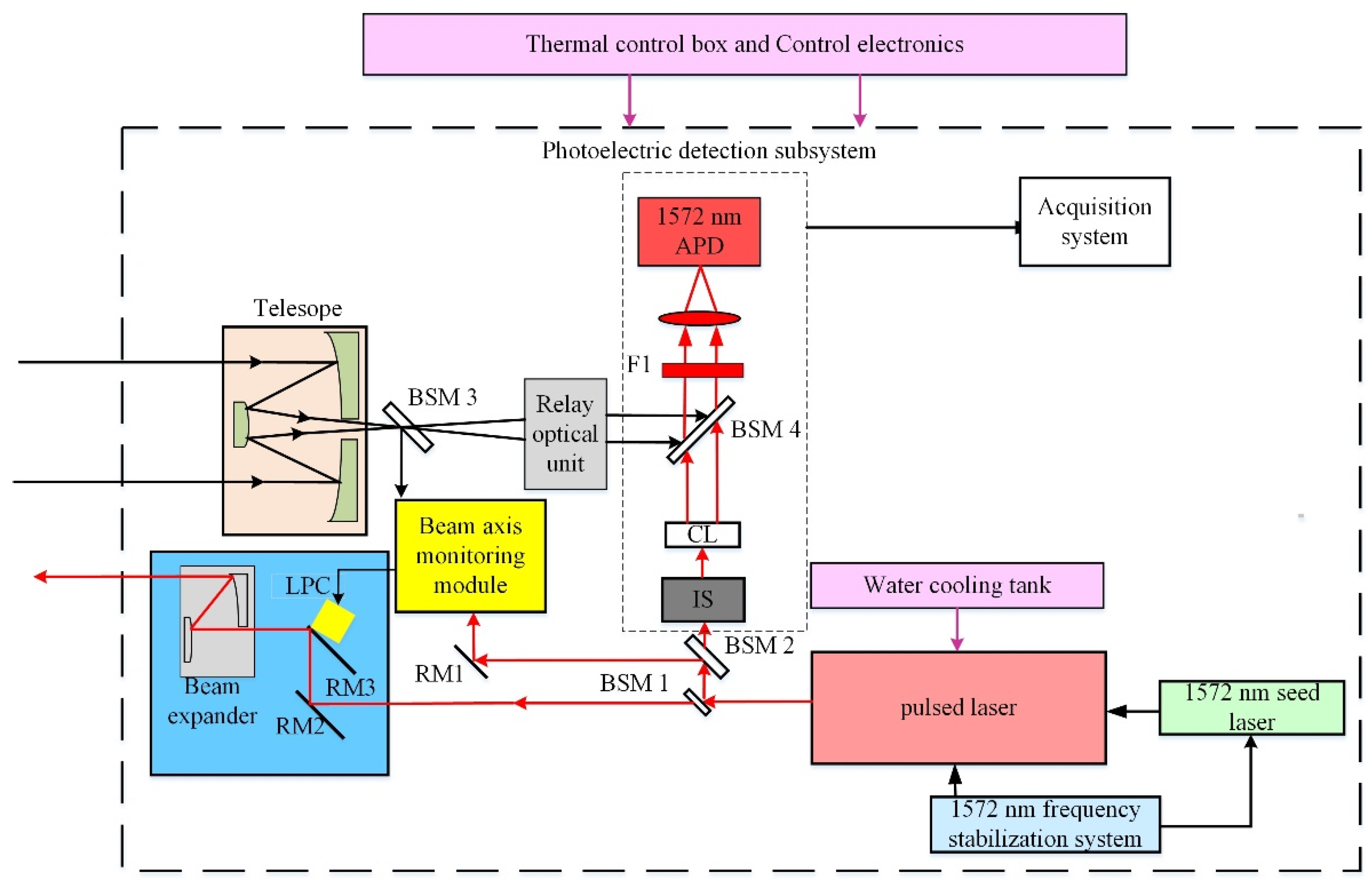
2. Spaceborne IPDA LIDAR Instrument and Principle

The active instrument for detecting carbon dioxide, clouds, and aerosols is called aerosol and carbon detection LIDAR (ACDL). Figure 1 shows the schematic diagram of the IPDA LIDAR system of ACDL for CO₂ measurement. The transmitted laser of the IPDA LIDAR system requires 1572 nm high-energy laser pulses with high-frequency stability. There are many methods to stabilize laser frequency [21,22]. The 1572 nm seeder laser, 1572 nm frequency stabilization system, and the pulsed laser together generate the double-pulsed 1572 nm with frequency stability less than 0.60 MHz [23,24]. Beam splitter mirror 1 (BSM1) divides the 1572 nm laser pulse into two parts. One part of the laser pulse enters the atmosphere through the beam expander, and the other part is reflected into the monitoring system. The monitoring system includes a beam axis monitoring module and an energy monitoring module. To improve receiving efficiency, the beam axis monitoring module makes the optical axis of the emitted light consistent with the optical axis of the telescope. The energy monitoring module is composed of an integrating sphere (IS), an optical fiber, and a collimator lens (CL), which is used for accurate monitoring of emitting laser energy. The echo signals are received by the telescope and 1572 nm avalanche photodiode (APD) detector. The main parameters of the spaceborne IPDA LIDAR system are listed in

Table 1. System parameters of the spaceborne IPDA LIDAR.

Category	Parameter	Value
1572 nm Laser Transmitter	Wavelength (On-/offline)	1572.024/1572.085 nm
	Energy (On-/offline)	75/35 mJ
	Pulse width	15 ns
	Repetition frequency	20 Hz
	Pulse separation	200 μs
	Linewidth	30 MHz
	Frequency stability	0.6 MHz
	Spectral purity (OPA)	0.9995
Transceiver optics	Emission optical efficiency	0.9558
	Beam divergence	100 μrad
	Energy monitoring accuracy	0.9993
	Receiver optical efficiency	0.7186
	Telescope diameter	1 m
	Field of view	0.2 mrad
	Optical filter bandwidth	0.45 nm
APD Photoreceivers	Detector type	InGaAs APD
	Responsivity	4 MV/W@M = 10&RL = 50 Ω)
	APD NEP	33 fw/√Hz (@5 °C)
	Excess noise factor	5.5 (@M = 10)
	APD Bandwidth	8.9 MHz
ACB	Small gain channel	10 times
	High gain channel	60 times
	Bandwidth	1 MHz
	NEP at 10 times	38 nV/√Hz
Data acquisition (DA)	Sampling rate for 1572 nm	50 MS/s
	Effective numbers of bit	11 bits
	Voltage range	2 V
Satellite Platform	Orbit altitude	705 km
	Spatial resolution of land	50 km
	Spatial resolution of sea	100 km

.

Figure 2 shows the timing relationship of return signals (including monitoring and echo pulses) and schematic diagram of 1572 nm detector for the spaceborne IPDA LIDAR. Monitoring pulses are online and offline pulses with a time interval of 200 μs and an energy ratio of about 2:1. Echo pulses are received by the telescope after being reflected by the target. The online echo pulse is attenuated by trace gas molecules during propagation through the atmosphere. In contrast, the offline echo pulse is only weakly attenuated because it is far away from the center of the absorption line [25].

Without considering the ground fluctuations, the width of laser pulses before reaching the detector is about 15 ns. Due to the satellite altitude of 705 km, the time interval between the echo pulse and the monitoring pulse is about 4.7 ms. When laser pulse is focused on the APD photosensitive surface, photoelectric conversion occurs. The APD photoreceiver is widely used in various fields [16,26,27]. The preamplifier is a reverse amplifier with a bandwidth of 8.9 MHz. Therefore, after the APD photoreceiver, the signal is reversely broadened to about 40 ns. A fifth-order active filter is used to filter the signal and improve the linearity of the ACB. Finally, through CADENCE simulation, the optimized ACB bandwidth is designed as 1 MHz. After optimizing the ACB, the signal is further broadened to about 390 ns.

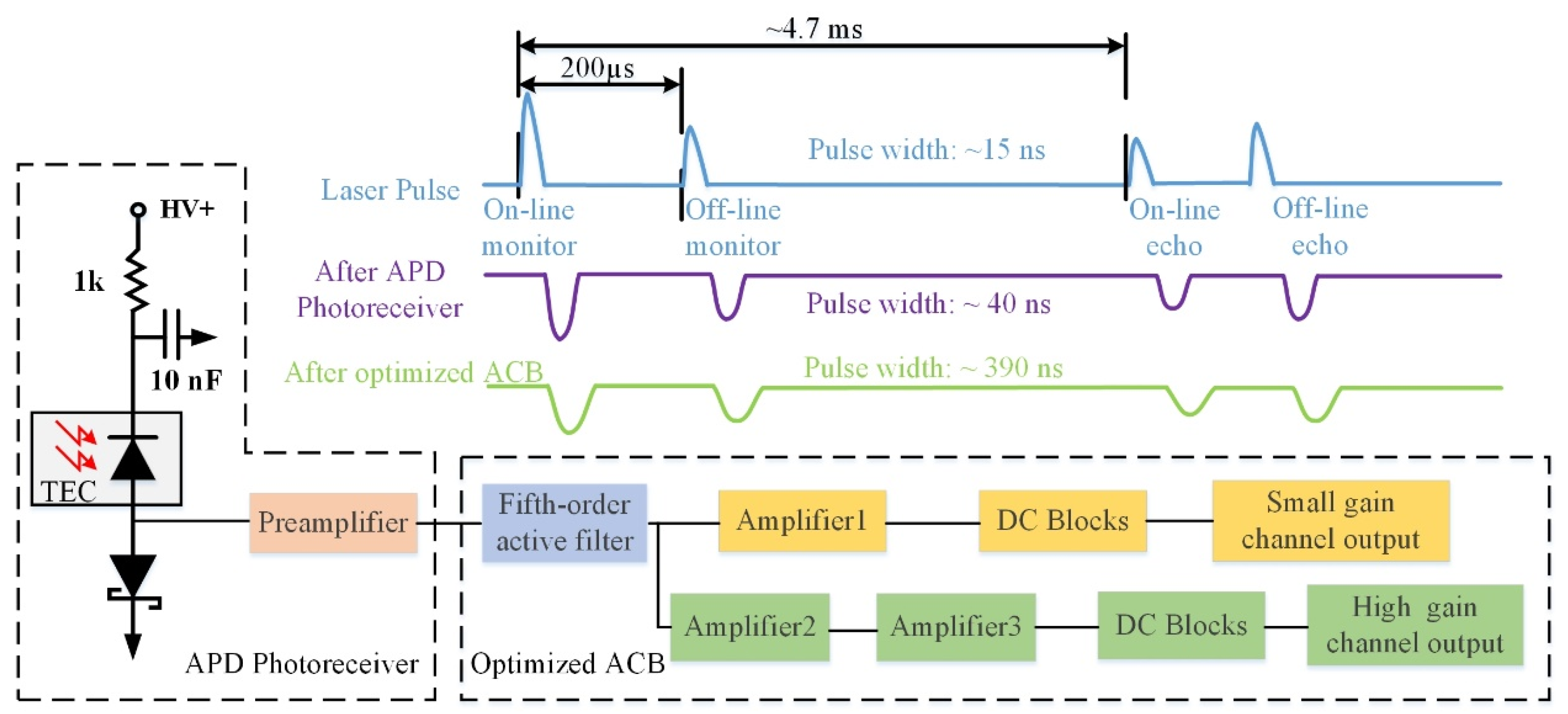
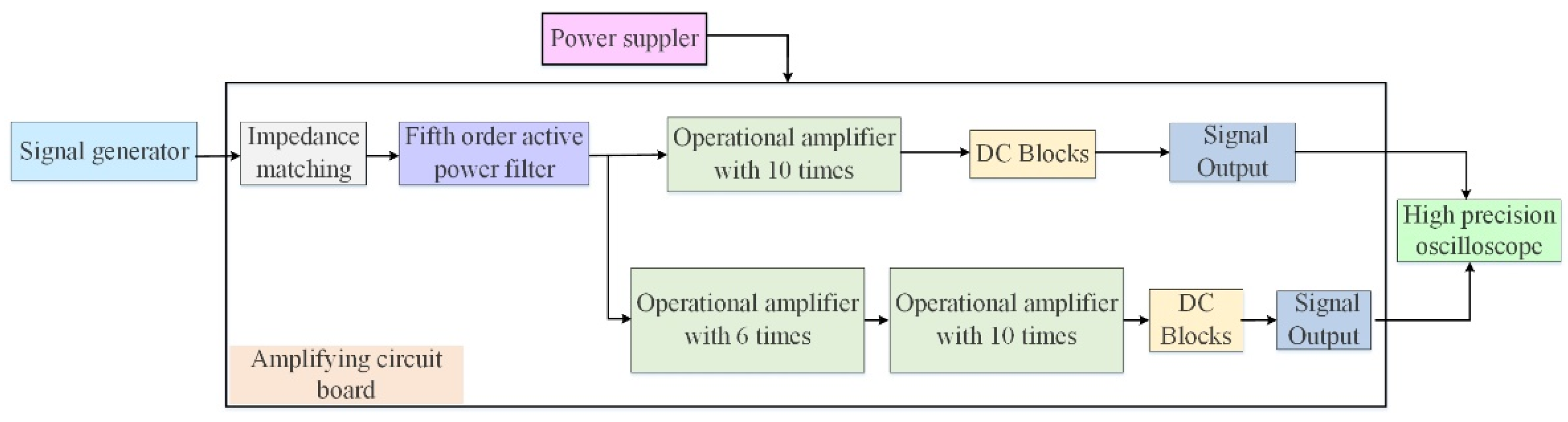
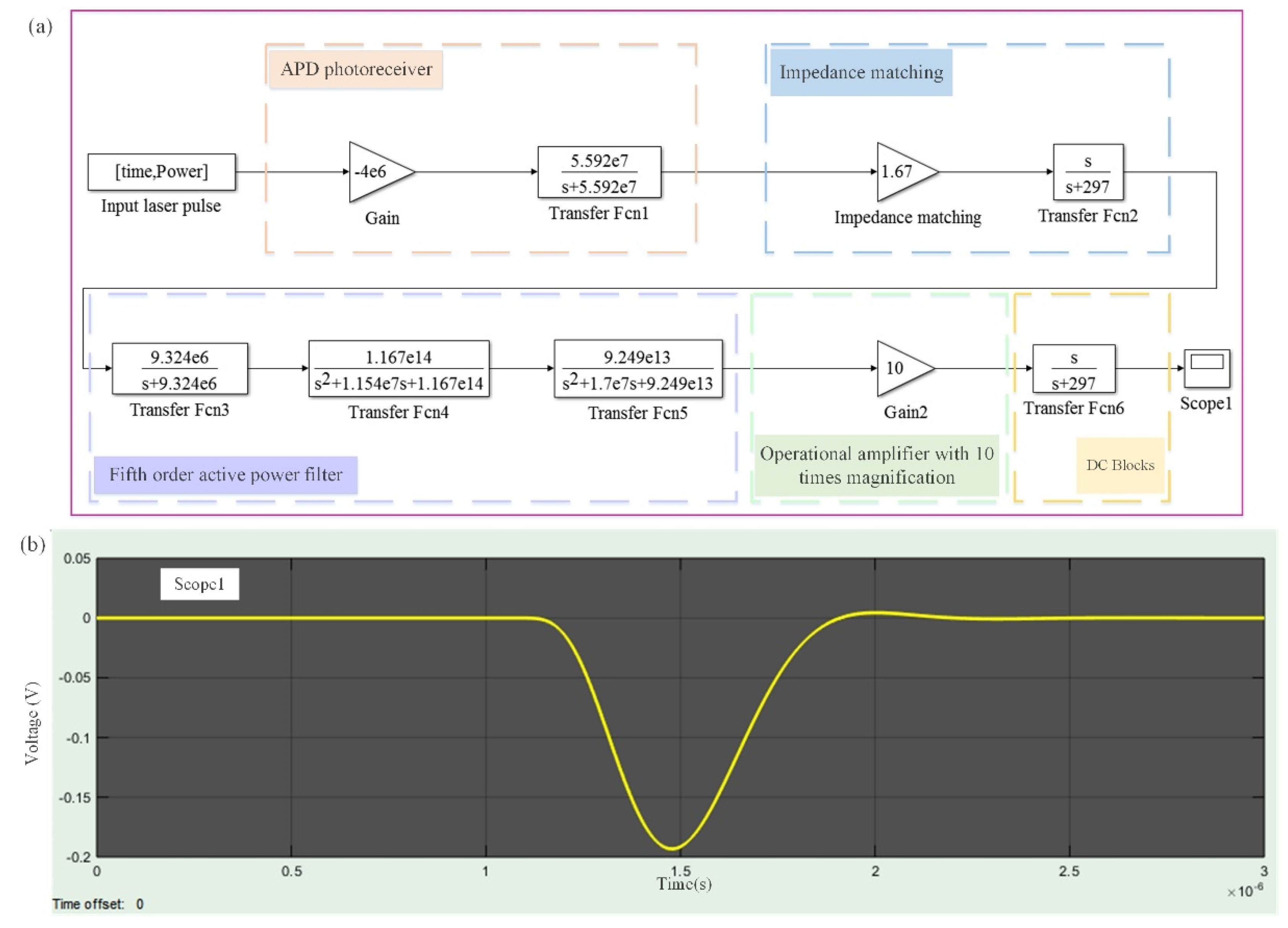
3. Optimization of Linearity and Amplification of the ACB

The nonlinearity of detector is not mentioned in many spaceborne IPDA LIDAR simulations [16,17,18,19,20]. However, due to the great variation in surface reflectance, the amplitude of the echo signal may vary greatly. Therefore, detector linearity is an important factor to determine the detection accuracy of the spaceborne IPDA LIDAR. There are two methods to improve detector linearity: One is to optimize the detector hardware to meet the requirement of linearity in the required dynamic range; the other is to calibrate the nonlinear curve of the detector in the required dynamic range and to correct the measured data. The second method will lead to the complexity of the inversion algorithm. Therefore, we chose the first method to optimize the ACB of the detector. First, the peak of laser pulse power before reaching the detector is simulated under different surface reflectance and atmospheric transmittances. Second, the ACB is designed to meet the requirement of linearity in the dynamic range of peak power, and the transfer model of the detector module is established by SIMULINK and CADENCE. The linearity before and after optimization is compared through simulation and experiment.

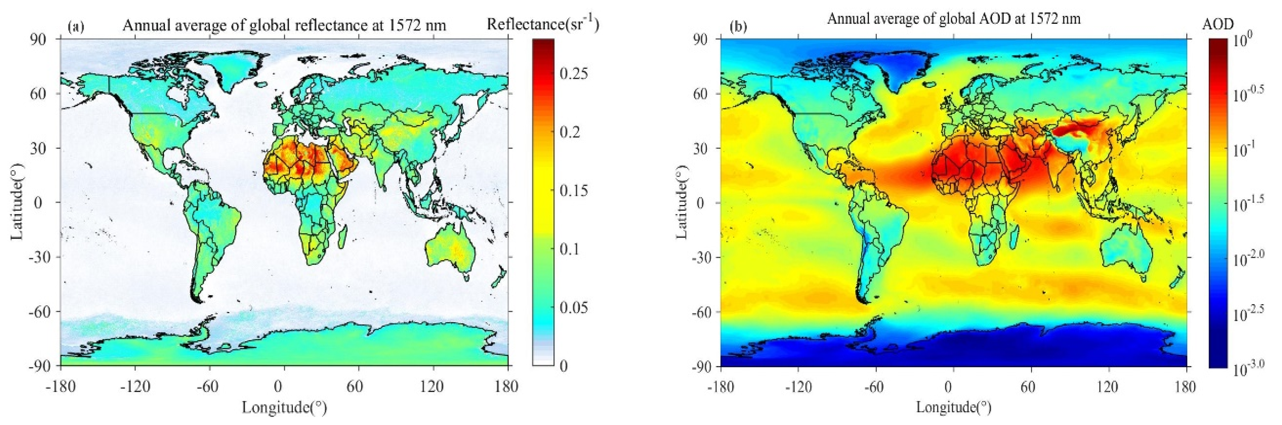
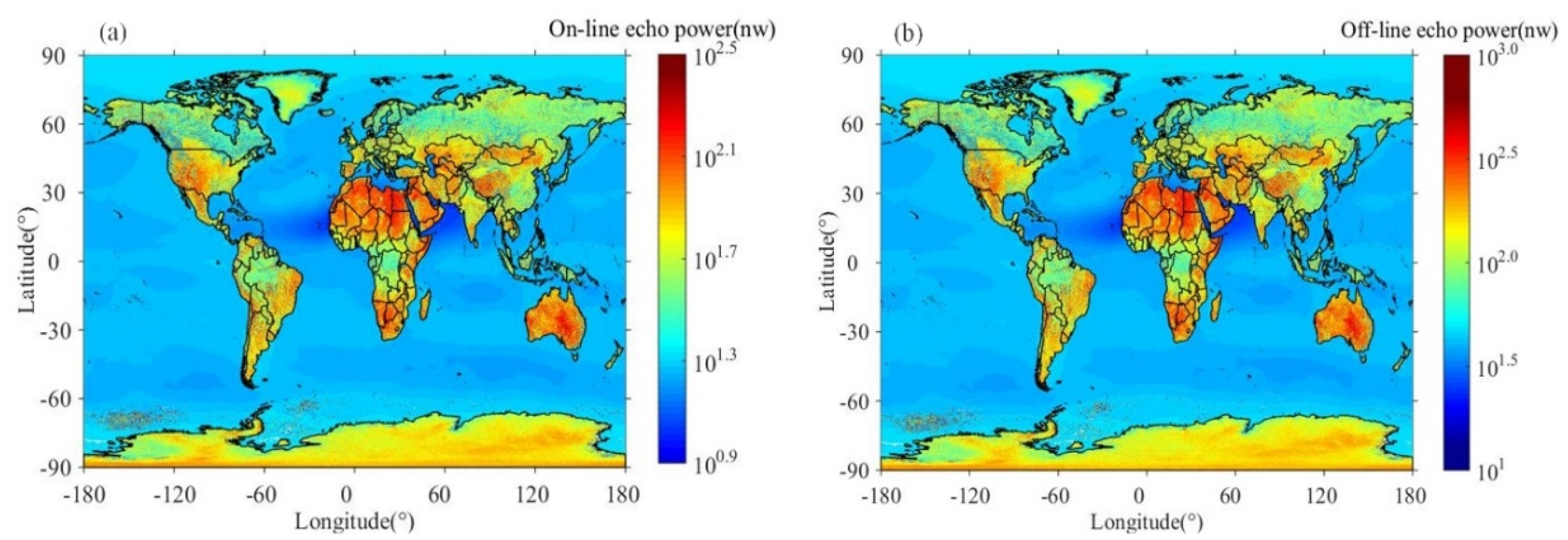
3.1. Dynamic Range of the Global Echo Signal

Echo signal power can be calculated by the hard target LIDAR equation [28], which can be written as

$$P_e(\lambda ,R_A)={\eta }_r\cdot O_r\cdot \frac{A}{{\left(R_A-R_G\right)}^2}\cdot \frac{E(\lambda )}{\Delta t(\lambda )}\cdot {\rho }^{*}\cdot T_m\cdot \exp [-{\tau }_{C{O}_2}(\lambda ,R_A)]$$

(1)

where $P_e$ is the echo signal power, ${\eta }_r$ is the product of emission and receiver optical efficiency, $O_r$ is the overlap function, $A$ is the area of the telescope, $R_A$ is the satellite altitude, $R_G$ is the altitude of the hard target above sea level, $E$ is the transmitted laser energy, $\Delta t$ is the effective pulse width of the return pulse, ${\rho }^{*}$ is the target reflectivity defined as the reflected power per steradian toward the receiver divided by the incident power [3], ${\tau }_{C{O}_2}$ is the total integrated double-path optical depth caused by atmospheric CO₂ molecules, and $T_m$ is the atmospheric transmission efficiency. Here, we assume that the altitude of the hard target is 0 km.

The surface reflectance of 1572 nm can be obtained by interpolating band 6 (1628~1652 nm) and band 7 (2105~2155 nm) of the moderate-resolution imaging spectroradiometer (MODIS) [29,30]. The central wavelength of band 6 is 1640 nm, and the central wavelength of band 7 is 2130 nm. The reflectance of 1572 nm can be calculated by [30]

$${\rho }_{1572\mathrm{nm}}=0.727\cdot {\rho }_{1640\mathrm{nm}}+0.309\cdot {\rho }_{2130\mathrm{nm}}$$

(2)

where ${\rho }_{1640\mathrm{nm}}$ and ${\rho }_{2130\mathrm{nm}}$ are the reflectance of 1640 nm and 2130 nm, respectively. Figure 3a shows the annual average of global surface reflectance in 2018. The atmospheric transmission efficiency at 1572 nm is mainly caused by the absorption of atmospheric aerosols. The aerosols optical depth (AOD) at 1572 nm can be calculated by the relationship between AOD and Angstrom’s exponent at two known wavelengths. Figure 3b shows the annual average of global AOD at 1572 nm in 2018. The total integrated double-path optical depth caused by atmospheric CO₂ molecules is calculated from an assumed CO₂ column-averaged dry-air mixing ratio (XCO₂) of 400 ppm and the spectroscopy database HITRAN 2016 [31]. Furthermore, the echo power of online and offline signals calculated by Equation (1) is shown in Figure 4. Figure 4 shows that the minimum echo power of the spaceborne IPDA LIDAR system is 10 nW and the maximum echo power is 690 nW. The dynamic range of echo signal power is approximately 70.

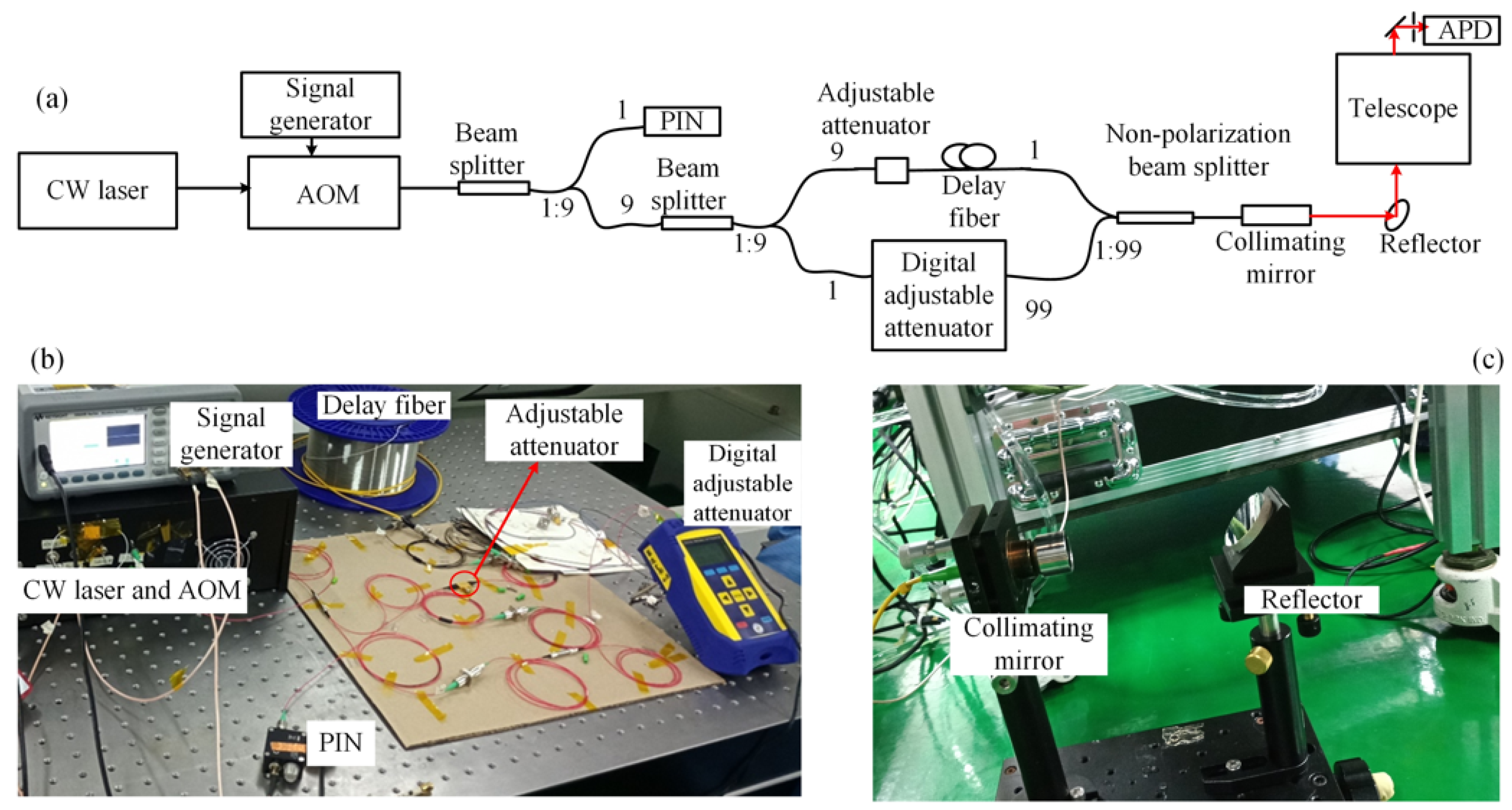
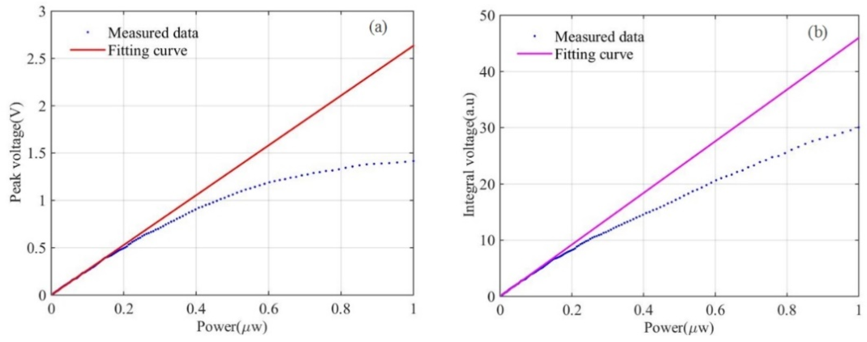
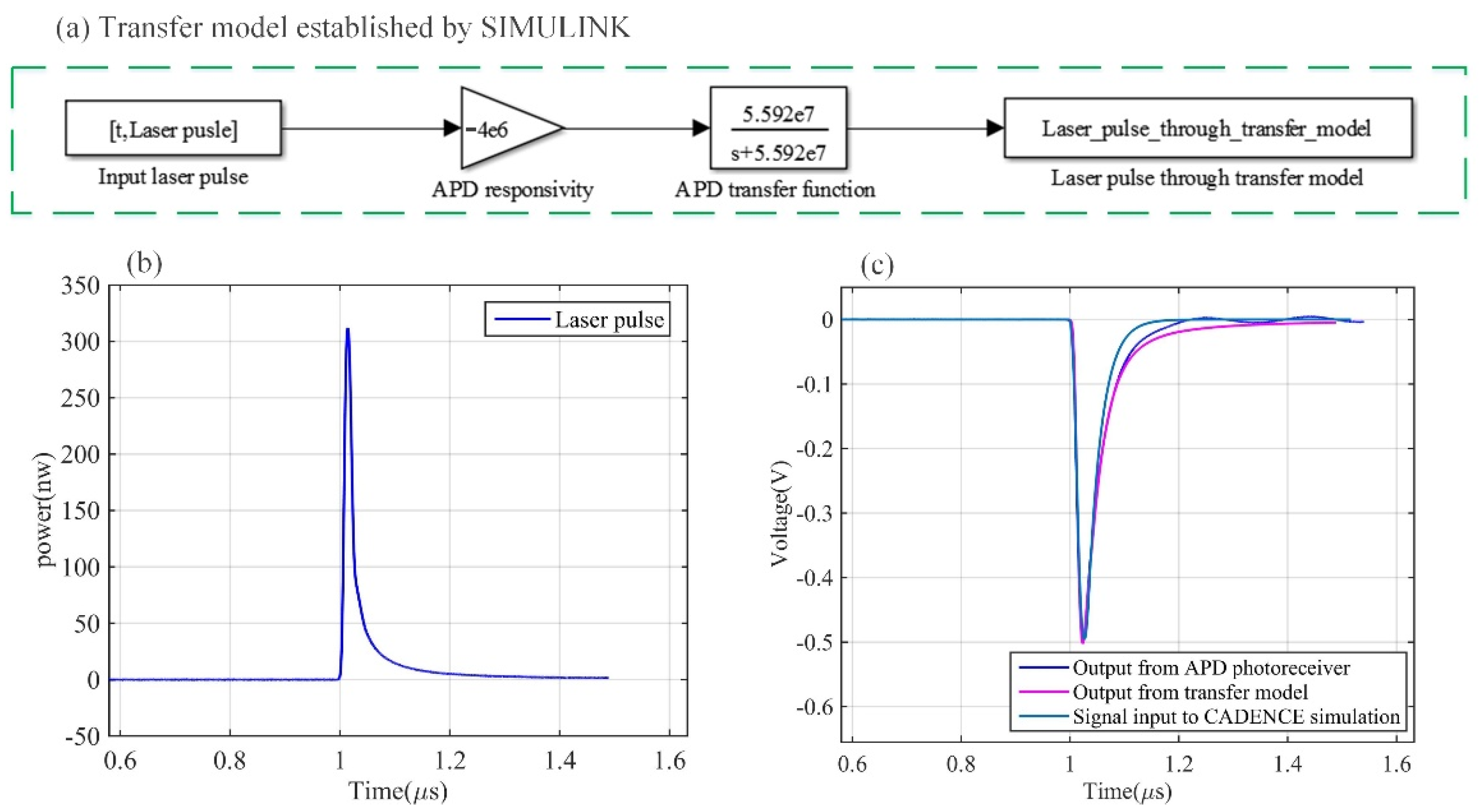
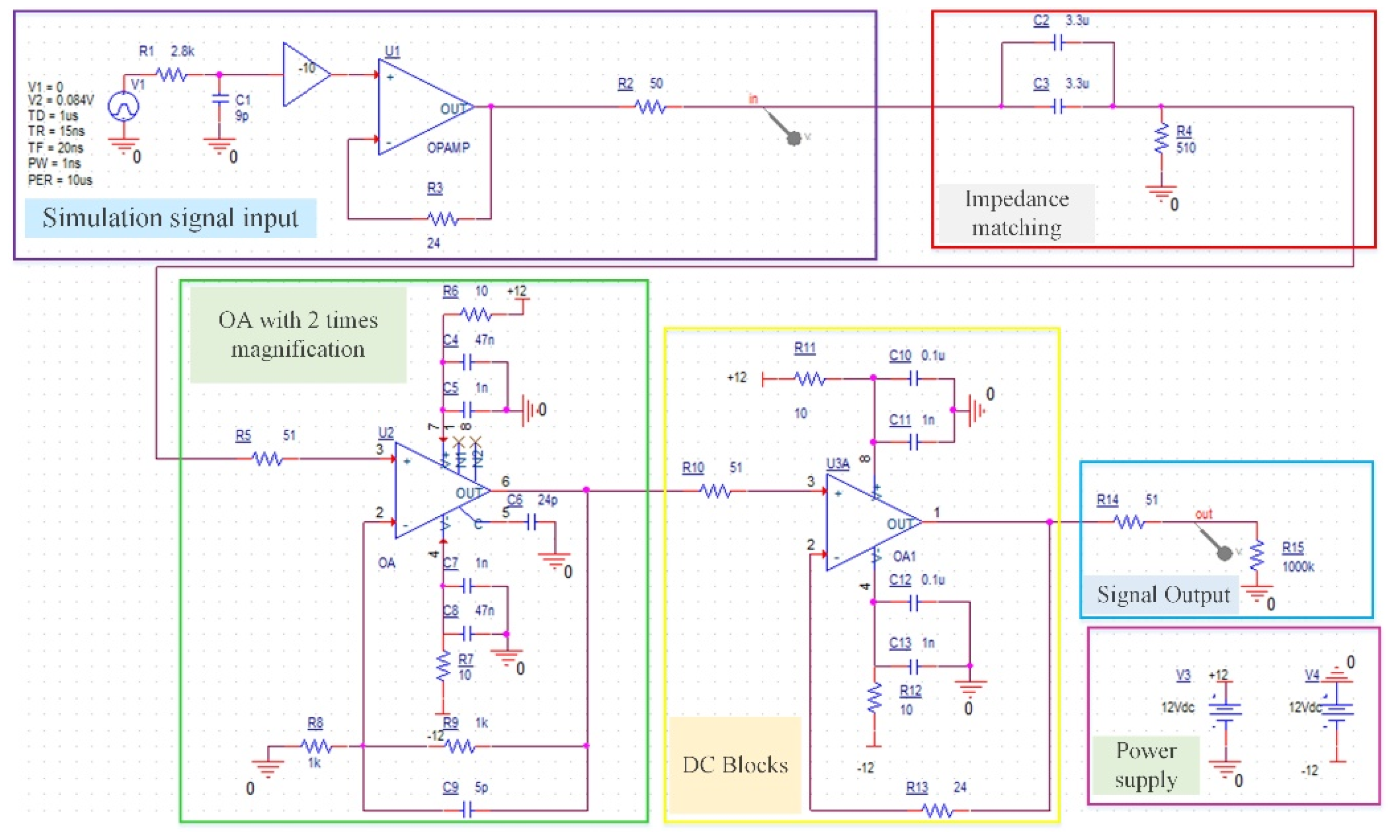
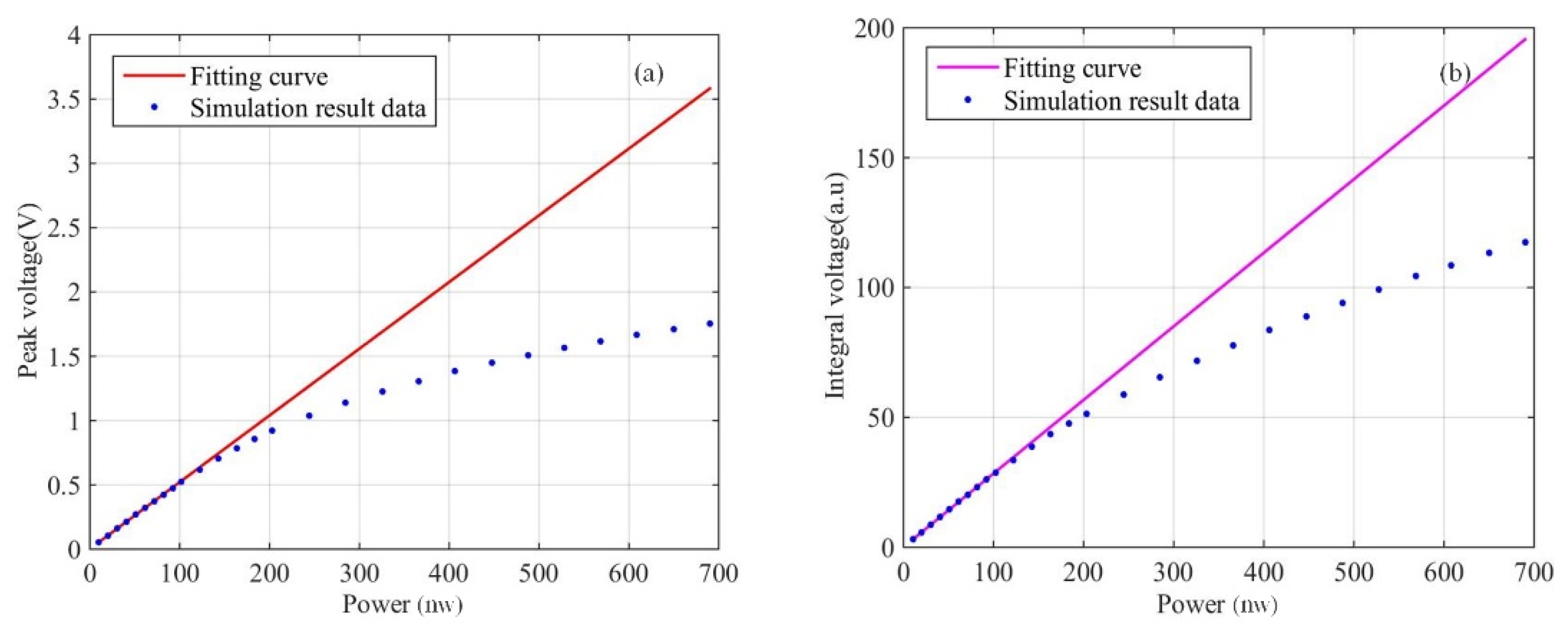
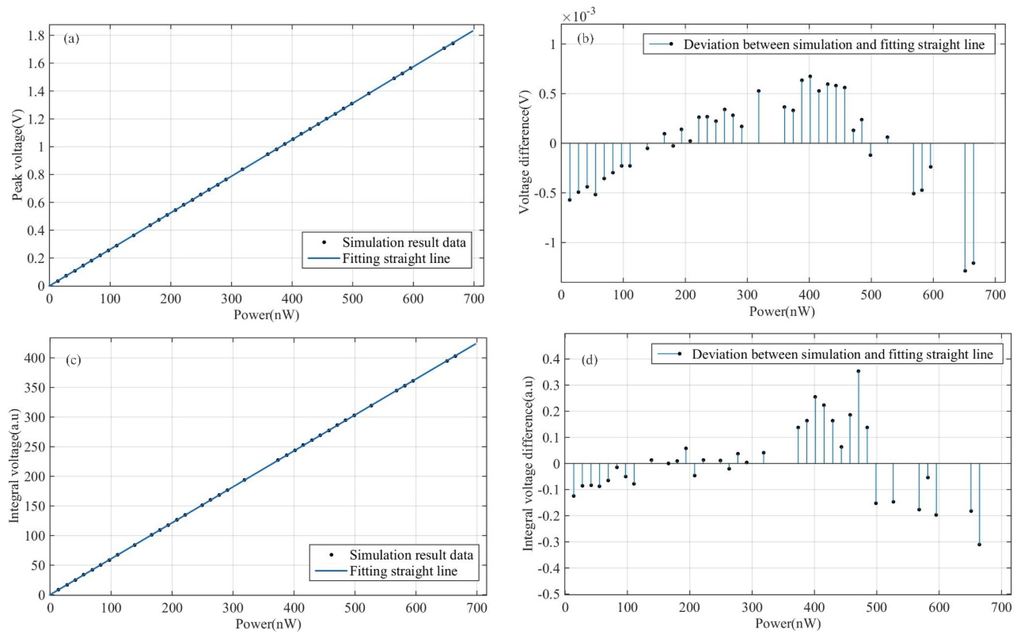
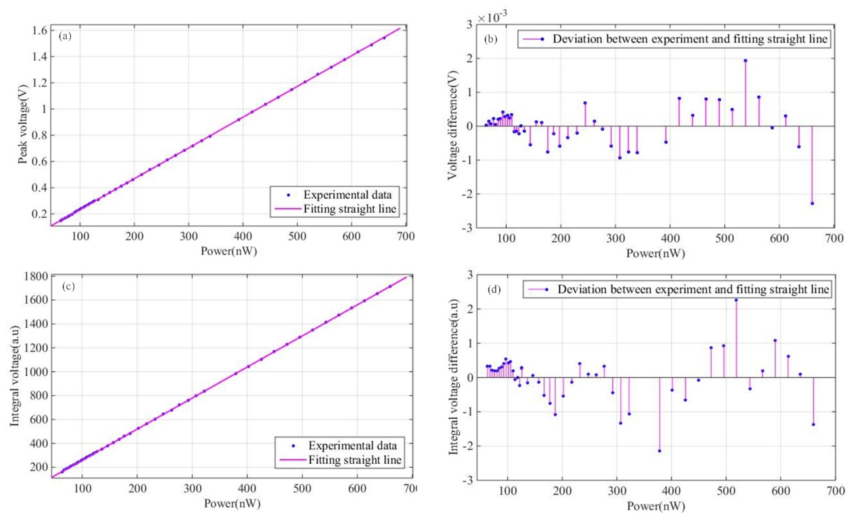
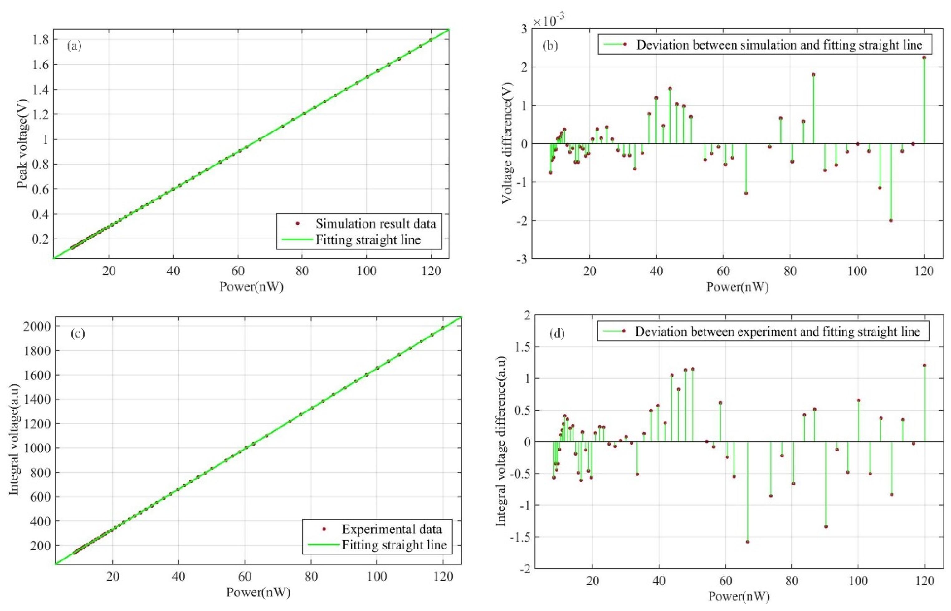
3.2. Linearity Simulation and Test

In the airborne experiment, a problem of data inversion caused by nonlinearity was found [20]. The signal with peak voltages greater than 400 mV could not be used to retrieve CO₂ with high accuracy. Figure 5 shows the detector linearity test setup and instruments. Figure 6a shows the output peak voltage of the airborne prototype detector varying with input power. Figure 6b shows the output integral voltage of the airborne prototype detector varying with the input power. The actual output voltage in Figure 6 is negative. For descriptive convenience, the absolute values of output peak and integral voltage are taken here. The integral voltage value is obtained by adding the voltages of all points on the pulse, and its value depends on the sampling rate. Figure 6 proves that when the peak voltage is greater than 400 mV, there is a serious nonlinear phenomenon. The expression of linearity is

$$\delta =\frac{\Delta Y_{\max }}{Y}\times 100\%$$

(3)

where $\Delta Y_{\max }$ is the maximum deviation between the output curve and the fitting line, and $Y$ is the full scale output. The linearity in the dynamic range reaches 42.60%. Therefore, it is very important to find out the cause of nonlinearity and optimize the performance of detector to meet the requirement of linearity.

Through many experiments, the ACB of the detector was found to be the main factor causing nonlinearity. To optimize the ACB, SIMULINK and CADENCE software were used to model the detector. First, the transfer model of the APD photoreceiver is established by SIMULINK. Second, CADENCE software is used to simulate the output signal of the ACB. The APD photoreceiver converts a laser pulse into an electrical signal. The responsivity of the APD photoreceiver is 4 MV/W in its bandwidth range. Due to the narrow pulse width of the laser pulse, the frequency distribution of the converted signal is much larger than the bandwidth of the APD photoreceiver. Hence, the APD photoreceiver transfer model needs to be equivalent to the product of the response and transfer function. The transfer function can be expressed by

$$H(j\omega )=\frac{1}{1+\raisebox{1ex}{$j\omega $}\!\left/ \!\raisebox{-1ex}{$2\pi B$}\right.}$$

(4)

where $B$ is the bandwidth of the APD photoreceiver. Let $S=j\omega$, then

$$H(S)=\frac{2\pi B}{S+2\pi B}$$

(5)

Therefore, the transfer model of the APD photoreceiver can be expressed as Figure 7a. Figure 7b shows a laser pulse which is used to verify the accuracy of the transfer model. The laser pulse waveform was detected by a broadband detector and the laser pulse power was detected by a dynamometer. The blue line in Figure 7c is the direct output signal of the laser pulse passing through the APD photoreceiver, and the red line is the simulated signal of the laser pulse passing through the transfer model. It can be seen from the figure that the blue line and the red line are very consistent, which proves the accuracy of the transfer model.

In order to detect accurately in this dynamic range, the noise of the amplifier chip and the linearity of the signal response should be considered simultaneously. The high-speed, low-noise operational amplifier (OA) was selected as the amplifier chip. On the basis of the original airborne ACB design, CADENCE simulation at twice amplification is carried out for the ACB of spaceborne IPDA LIDAR, as shown in Figure 8. The CADENCE simulation for ACB consists of six parts: simulation signal input, impedance matching, OA, DC blocks, signal output, and power supply. The cyan line in Figure 7c is generated by the simulation signal input part in Figure 8, which is almost consistent with the blue line in Figure 7c. The green line (the same as the cyan line in Figure 7c) and the red line in Figure 9 are the input signal and output signal of the ACB in simulation. Combining the APD photoreceiver model in Figure 7a with the CADENCE simulation of ACB in Figure 8, we can get the output voltage of the detector when it changes with input power. Figure 10 shows the curve of the output voltage changing with the input power. In the simulation, the transfer function $H(S)$ of the APD photoreceiver is linear. By comparing the curve change trend in Figure 10 with Figure 6, it can be concluded that the ACB is the main factor leading to the nonlinearity of the IPDA LIDAR system.

After a detailed analysis of the ACB, the nonlinear problem has been located. Figure 11a shows the optimized ACB. The optimization adds a fifth-order active power filter with 1 MHz bandwidth in front of the OA. This reduces the slew rate requirement of the OA so that the optimized ACB can meet the requirement of linearity. Figure 11b shows the output waveform of the optimized ACB. Because the fifth-order active power filter reduces the peak value of the signal, the amplification factor of the OA is increased to adapt to the voltage range of the DA. Figure 12a shows the simulated output peak voltage of the optimized ACB varying with input power. When the maximum power is 690 nW, the corresponding output peak voltage is about 1.70 V. As can be seen from Figure 12b, the maximum voltage deviation between the simulation data and the fitting curve is −1.27 mV. Therefore, the output peak voltage linearity of the optimized ACB is 0.0747%. Figure 12c shows the simulated integral peak voltage of the optimized ACB varying with input power. The sampling interval used in the CADENCE simulation is 1 ns. According to Equation (3) and Figure 12d, the output integral voltage linearity of the optimized ACB is 0.0877%.

The CADENCE simulation results show that the linearity of the optimized ACB meets the requirements of IPDA LIDAR detection. For further verification, the optimized ACB is produced according to the CADENCE design, and its linearity is verified by experiment test. Figure 13 shows the test flow chart. The input of the optimized ACB is given by a signal generator, and incident light power change is simulated by changing the output amplitude of the signal generator. The output of the signal generator is sent to the optimized ACB. The optimized ACB has two channels to amplify the signal, and finally output to a high-precision oscilloscope for signal acquisition. The high-precision oscilloscope has 12 effective bit numbers, and the sampling rate reaches 3.125 GS/s. To reduce the influence of error, we chose the oscilloscope mode with the highest precision. The small gain channel is responsible for amplifying the signal with high echo power (from 55 nW to 700 nW), and the large gain channel is responsible for amplifying the signal with weak echo power (from 10 nW to 120 nW). The design reduces the influence of quantization noise on weak signals.

Figure 14 and Figure 15 show the test results in small and large gain channels, respectively. The optimal amplification of the small gain channel is 10 times, and that of the large gain channel is 60 times. However, due to individual differences of devices in the actual production process, such as error between the actual value and the nominal value of resistance of ±5%, or no resistance is equal to the design value, there may be a 10% error between the amplification and the design value. This does not affect the performance of the optimized ACB. Using Equation (3) and Figure 14, the output peak voltage linearity of the small gain channel is calculated as 0.149% and the output integral voltage linearity is 0.135%. Using Equation (3) and Figure 15, the output peak voltage linearity of the large gain channel is 0.127% and the output integral voltage linearity is 0.085%. Small changes in the instrument and environment during the experiment will lead to poor results. Therefore, compared experimental results with simulation results, the linearity of the optimized ACB can meet the detection requirements. The optimal amplification is determined in the simulation process, which is 10 times in the small gain channel and 60 times in the large gain channel. To avoid the state change of the spaceborne IPDA LIDAR system during operation, we set four gain levels. The small gain channels are 5 times, 10 times, 15 times, and 20 times, and the large gain channels are 30 times, 60 times, 90 times, and 120 times.

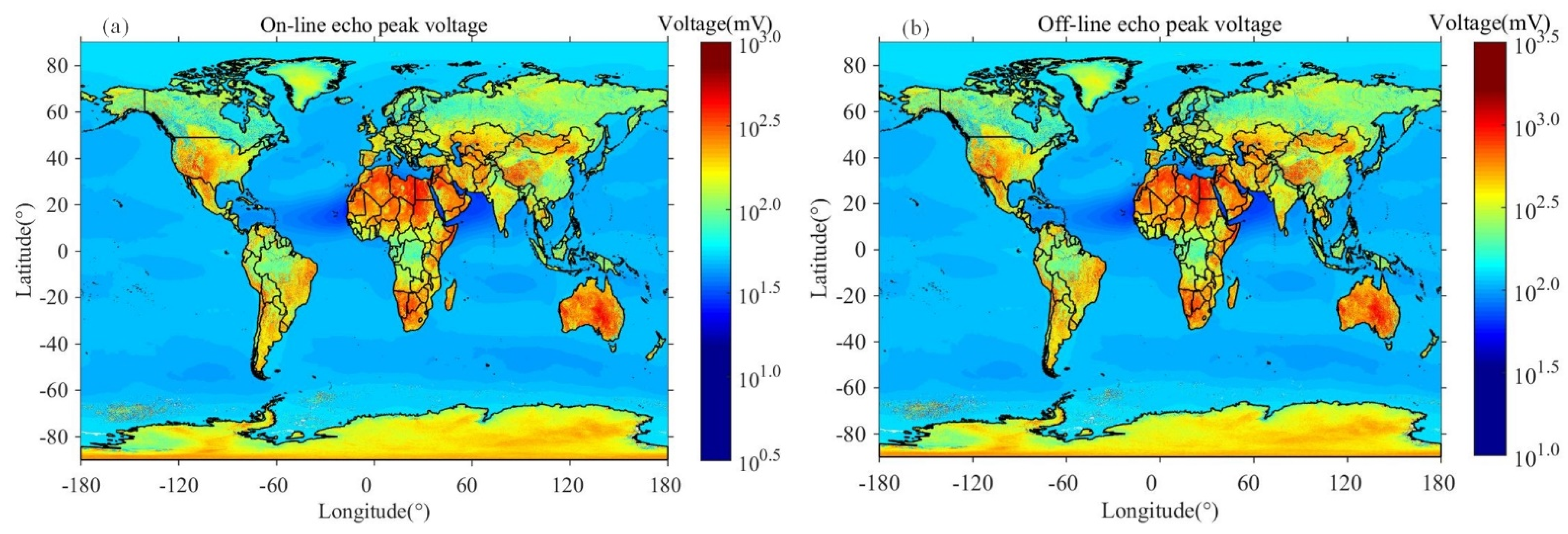
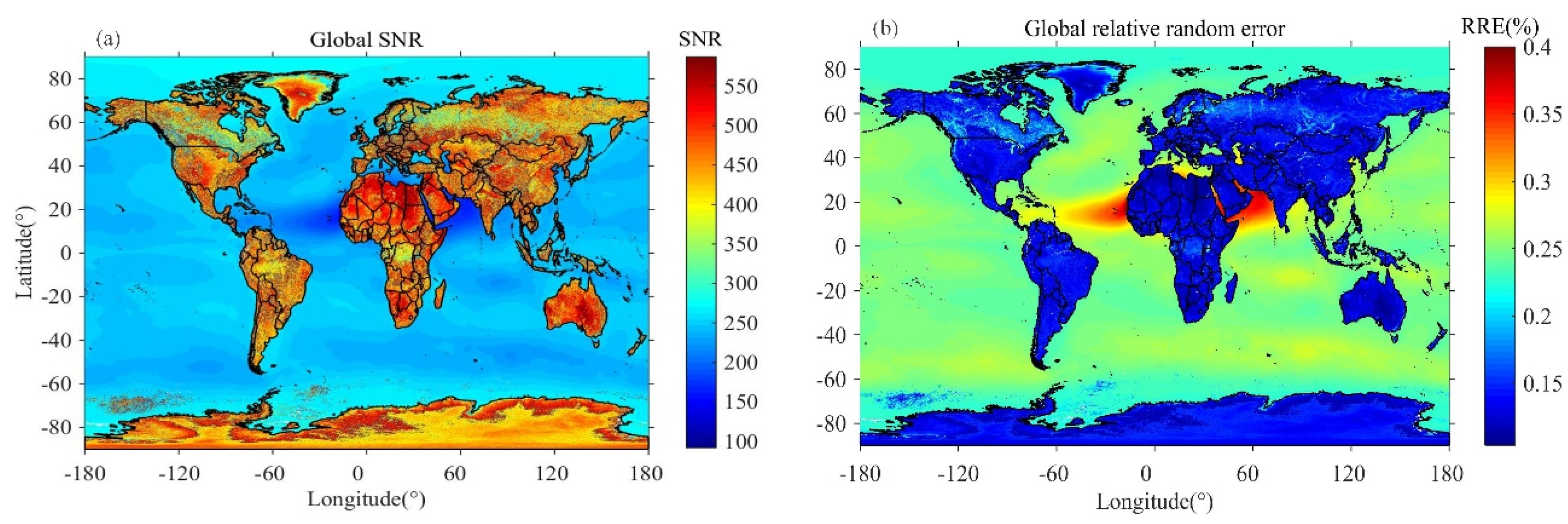
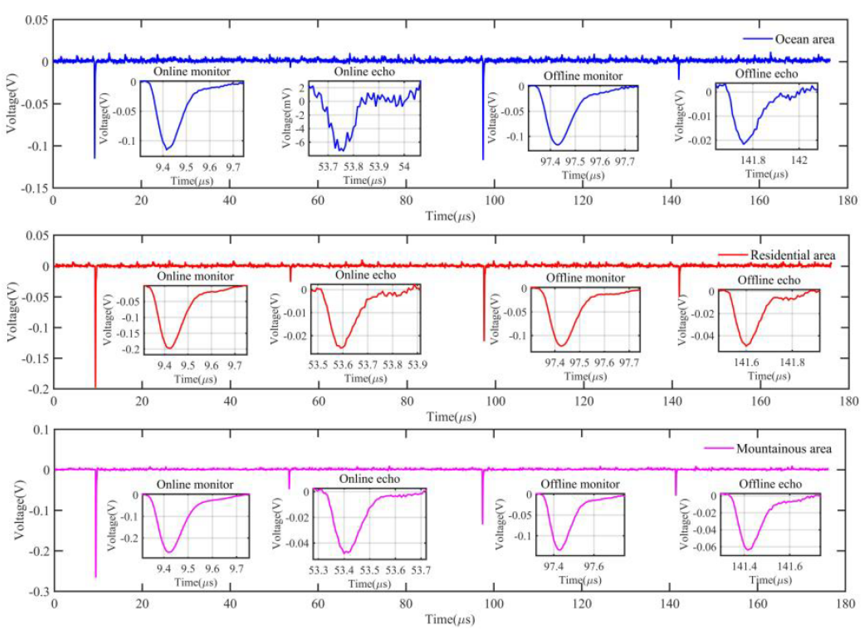
4. System Performance of Spaceborne IPDA LIDAR

Several groups have analyzed the performance of the IPDA LIDAR system [18,19,32], including the influence of system error on precision. However, effects on accuracy caused by nonlinearity have not been studied. The system performance of spaceborne IPDA LIDAR depends on detection accuracy and precision. Nonlinearity of the detector is the main factor affecting the inversion accuracy of the system, whereas random and systematic errors are the main factors affecting inversion precision. The output waveform of the optimized ACB changes obviously, which will affect the RE of the optimized IPDA LIDAR system. Therefore, after detector linearity is optimized to meet accuracy requirements as described in Section 3, the impact of RE on the precision of the optimized system should be analyzed again. Compared with the relative systematic error (RSE) simulation results of Han and Wang [18,19], there is no obvious change in other aspects, except that the spectral purity of the laser transmitter is optimized to 99.95%. The detector optimization in this paper does not affect the RSE. Therefore, RSE analysis is not repeated here.

When the gain (M) of APD photoreceiver is 10, and the amplification (F) of optimized ACB is 10, the peak voltages of the online and offline monitoring signals are set to 1.40 V and 0.70 V, respectively. According to the detector model in Section 3, the peak voltages of online and offline echo pulses are in the range of 0.025–0.78 V and 0.055–1.70 V, respectively. Figure 16 shows the global online and offline echo peak voltage distributions. Signal noise, background noise, APD photoreceiver noise, ACB noise, and quantization noise are the main factors causing RE. The expressions of these noises are given by Ehret et al. [25] and Kiemle et al. [33]. The calculation of noise is not repeated here. Because signal noise and background noise are related to the intensity of light, they are affected by surface reflectance and atmospheric transmittance. Figure 17 shows the global signal noise distribution of online and offline echo signals, and global background noise distribution. When the high voltage of the APD photoreceiver is constant, the APD photoreceiver noise is constant. The noise of the ACB varies linearly with its amplification. When the measurement range of the DA remains unchanged, the quantization noise is also a fixed value.

Table 2. The values of four signals and all noise sources at M = 10, T = 5 °C and F = 10.

Laser pulse (@M = 10, F = 10)	Peak Voltage	Unit
Online monitoring	1.40	V
Offline monitoring	0.70
Online echo	0.025–0.78
Offline echo	0.055–1.70
Noise (@M = 10, T = 5 °C, F = 10)	STD	Unit
Signal noise	1.40–12.0	mV
Background noise	0.39–1.80
APD photoreceiver noise	2.00
ACB noise	0.38
Quantization noise	0.98

shows the values of four signals and all noise sources.

The SNR is an important index of the evaluation system. The SNR for signals can be expressed as

$$SN{R}_i=\frac{V_i}{\sqrt{V_{N_S}^2+V_{N_B}^2+V_{N_A}^2+V_{N_C}^2+V_{N_Q}^2}}$$

(6)

where $i$ represents online monitoring, offline monitoring, online echo or offline echo signal; $V_i$ is the peak voltage of each signal; $V_{N_S}$ represents the signal noise; $V_{N_B}$ represents the background noise; $V_{N_A}$ represents the APD photoreceiver noise; $V_{N_C}$ represents the ACB noise; and $V_{N_Q}$ represents the quantization noise. Because the noise is uncorrelated, the total SNR can be expressed as

$$\frac{1}{SN{R}_{total}}=\sqrt{{\displaystyle \sum _i\frac{1}{SN{R}_i^2}}}$$

(7)

When land and ocean spatial resolutions are 50 km and 100 km, respectively, the corresponding average times can be calculated as 148 and 296 pulses, respectively. The number of pulses is calculated according to satellite speed and the laser transmitter repetition frequency. The final SNR can be expressed as

$$SNR=SN{R}_{total}\cdot \sqrt{N_{shot\mathrm{s}}}$$

(8)

where $N_{shot\mathrm{s}}$ is the number of pulses. Figure 18a shows the global SNR calculated using MODIS data and cloud-aerosol LIDAR and infrared pathfinder satellite observation (CALIPSO) data from 2018. The relative RE (RRE) in XCO₂ can be approximated as

$$\frac{\delta XC{O}_2}{XC{O}_2}\approx \frac{1}{\Delta {\tau }_{C{O}_2}\cdot SN{R}_{total}\cdot \sqrt{N_{shot\mathrm{s}}}}$$

(9)

where $\Delta {\tau }_{C{O}_2}$ is total integrated double-path differential absorption optical depth caused by atmospheric CO₂ molecules. Figure 18b shows the corresponding global RRE. The proportion of RRE of different segments is listed in

Table 3. Proportion of RRE or different segments.

RRE (%)	$\mathit{\delta }\mathit{X}\mathit{C}{\mathit{O}}_2 \left(\mathbf{ppm}\right)$	Proportion
>0.3	>1.2	1.12%
0.25–0.3	1.0–1.2	25.66%
0.15–0.25	0.6–1.0	47.38%
<0.15	<0.6	25.84%

.

The analysis results in Table 3 are based on the MODIS annual average of global surface reflectance in 2018. According to the probability distribution of global surface reflectance in Figure 19 calculated by kiemle et al. using MODIS land data and GMAO sea surface data, the sea surface reflectance given in Figure 3a is low [34]. Because there are many clouds on the sea surface, and the effect of cloud removal is not good, the reflectivity of the sea surface processed by MODIS data may be low. Kiemle et al. gave that the area with surface reflectivity greater than 0.03 sr⁻¹ accounted for more than 90% of the world [34]. Using aerosol AOD distribution in Figure 3b for calculation, the sea surface reflectivity of 0.03 sr⁻¹ corresponds to an average RE of 0.182% (0.728 ppm). Therefore, more than 90% of the global RE can be less than 0.728 ppm.

5. Discussion

This paper analyzes the problem of nonlinearity, which is seldomly mentioned in system performance simulations of the spaceborne IPDA LIDAR [18,19]. Continuous hardware updating and iterating can achieve better system performance. For spaceborne IPDA LIDAR, the most important thing is the performance and lifetime of the transmitter and receiver. The performance of the detector also plays an important role in a long-term operation of the spaceborne IPDA LIDAR. The choice of detector is very difficult because it needs to maintain linearity and low noise in a large dynamic range. This paper presents the design and test method of a detector ACB, which has certain reference value for other LIDAR systems. An optimized detector has been installed, debugged and will be used in airborne experiments in the near future. Although the linearity of the ACB has been tested in the laboratory and can meet requirements, we are now preparing to use a test scheme similar to that in Figure 5 to test the linearity of the whole detector under the vacuum conditions of its future operation. After the spaceborne IPDA LIDAR launched, nonlinear curves under different pulse widths (due to surface fluctuations) will be given for data correction. This work helps improve the inversion accuracy of spaceborne IPDA LIDAR data in the future.

In prior system simulation work, the conversion process of the laser pulse in detector was unknown. According to LIDAR system parameters, only signal amplitude and the root mean square value of noise can be calculated. The actual pulse signal waveform and noise characteristics cannot be obtained from simulations. According to the principle of the optimized ACB in Section 3, the transfer model of the detector is established by SIMULINK, as shown in Figure 20a. The transfer function of impedance matching depends on the extent of matching with APD photoreceiver output impedance and first-order high pass filter characteristics. The first transfer function of the fifth-order active power filter is a first-order low-pass filtering characteristic, as shown in Equation (4). The second transfer function of the fifth-order active power filter is a second-order low-pass Sallen-key type filter, which can be expressed by

$$H_4(S)=\frac{1}{R_{27}\cdot R_{28}\cdot C_{28}\cdot C_{27}\cdot S^2+(R_{27}+R_{28})\cdot C_{27}\cdot S+1}$$

(10)

where $R_{27}$, $R_{28}$, $C_{28}$, and $C_{27}$ are the resistance and capacitance values in Figure 11a, respectively. The third transfer function of the fifth-order active power filter is expressed in the same way as Equation (10). Because the bandwidth of the fifth-order active power filter is the smallest, it determines the bandwidth of the whole ACB, and the OA can be directly regarded as its amplification. As shown in Figure 20a, the transfer function in SIMULINK replaces the corresponding part in Figure 11a. The output waveform from the transfer model in Figure 20b is consistent with that in Figure 11b. In this way, the simulation process is simplified, and the signal conversion process inside the detector can be completed using SIMULINK without learning CADENCE software. Using the transfer model of the detector to analyze the real pulse waveform and amplitude-frequency characteristics of noise, we can further study the inversion algorithm to improve inversion accuracy and precision.

Comparing the final output waveform of airborne experiments in Figure 21 with that of the optimized ACB in Figure 11, it can be seen that pulse shape and pulse width have changed significantly. This will affect the RE and data inversion algorithm of the optimized IPDA LIDAR system. In Section 3, system linearity is optimized to meet accuracy requirements, and linearity in the dynamic range is 0.0747% (0.30 ppm). In Section 4, the impact of RE on the precision of the optimized system is analyzed. The RRE of 25.84% of the global area is less than 0.15% (0.60 ppm). The RRE of 47.38% of the global area is between 0.15 and 0.25% (0.60–1.00 ppm), and the RRE of 25.66% of the global area is between 0.25 and 0.3% (1.00–1.20 ppm) Only 1.12% of the global area exceeded 0.3% RRE (1.20 ppm), mainly concentrated in the ocean near Africa due to its relatively high aerosol concentration. We require that the error of the land part should not exceed 0.60 ppm. Land accounts for about 29% of the global area, indicating that data efficiency is high. Kiemle concluded that more than 90% of the world’s surface reflectance is greater than 0.03 sr⁻¹. Through the performance simulation by the optimized system parameters and Kiemle’s conclusion, the RE of more than 90% of the global area is less than 0.728 ppm. Compared with the results of the airborne experiments in 2019 [20], the performance of optimized system has improved. Compared with the simulation results of Han et al. and Wang et al. [18,19], RE of the optimized IPDA LIDAR system does not increase. However, the influence of ground undulations on waveforms is not considered here, which needs to be analyzed in future research. It can be combined with the transfer model of the detector in Figure 20 to study the inversion algorithm or neural network learning to get better inversion results.

6. Conclusions

The airborne experiments of a scale prototype of China’s planned spaceborne IPDA LIDAR was implemented in 2019. A problem with data inversion caused by nonlinearity was found. The results of detector linearity tests show that when the peak voltage is greater than 400 mV, there is a serious nonlinear phenomenon. Through many experiments, it is found that the detector was the main factor causing the nonlinearity. In order to find the cause of the nonlinearity, SIMULINK and CADENCE software are used to model the detector. The model of APD photoreceiver is established by using SIMULINK. The model of ACB is established by CADENCE. Comparing nonlinear curve obtained from the simulation with experiments, it can be concluded that ACB is the main factor leading to the nonlinearity of the IPDA LIDAR measurement system.

According to the requirements of the spaceborne IPDA LIDAR system for CO₂ concentrations measurements, the ACB is optimized. First, the global echo signal power distribution is simulated using average annual surface reflectance and average annual aerosol concentration from other sensors in 2018. The minimum echo power of the spaceborne IPDA LIDAR system is 10 nW and the maximum echo power is 690 nW. The dynamic range of echo signal power is approximately 70. Second, the ACB is optimized by adding a fifth-order active power filter with 1 MHz bandwidth in front of OA. The purpose of this method is to reduce the slew rate requirement of the OA and make the optimized ACB meet the requirement of linearity. The CADENCE simulation results show that the output peak voltage linearity of the optimized ACB is 0.0747% and the output integral voltage linearity of the optimized ACB is 0.0877%. For further verification, the optimized ACB is produced, and its linearity is verified by experiments. To reduce the influence of quantization noise on weak signals, small gain channel and large gain channel are set in the optimized ACB. The signal is amplified 10 times in the small gain channel and 60 times in the large gain channel in the simulation. The output peak voltage linearity of the small gain channel is 0.149% and the output integral voltage linearity is 0.135%. The output peak voltage linearity of the large gain channel is 0.127% and the output integral voltage linearity is 0.085%. Because small changes of instruments and environments in the experimental process will lead to poor results, the simulation is taken as the final result. Therefore, the linearity of the optimized ACB in the dynamic range reaches 0.0747%, which is much better than the original version, with a linearity of 42.60%. The accuracy of the optimized IPDA LIDAR system can be controlled within 0.30 ppm. In order to avoid the influence of the state change of the spaceborne IPDA LIDAR system during operation, we set four gain levels. The small gain channels are 5, 10, 15, and 20 times, and the large gain channels are 30, 60, 90, and 120 times.

System performance of the spaceborne IPDA LIDAR depends on detection accuracy and precision. Nonlinearity of the detector is the main factor affecting the inversion accuracy of the system, while random and systematic errors are the main factors affecting inversion precision. The output waveform of the optimized ACB changes significantly, which will affect the RE of the optimized IPDA LIDAR system. Therefore, the global RE distribution of the optimized IPDA LIDAR system is simulated. Kiemle concluded that more than 90% of the world’s surface reflectance is greater than 0.03 sr⁻¹. Through the performance simulation by the optimized system parameters and Kiemle’s conclusion, the RE of more than 90% of the global area is less than 0.728 ppm. Finally, the transfer model of the detector module was given, which will be helpful for the further optimization of XCO₂ inversion algorithm.

7. Patents

An amplifier design circuit for avalanche photodetector, patent for invention, application No.: 202011039567.1 (2020).

References

1. Pachauri, R.K.; The Core Writing Team; Reisinger, A. Synthesis Report. Contribution of Working Groups I, II and III to the Fourth Assessment Report of the Intergovernmental Panel on Climate Change; Climate Change 2007; IPCC: Geneva, Switzerland, 2007; p. 104. [Google Scholar]
2. Stocker, T.F.; Qin, D.; Plattner, G.-K.; Tignor, M.; Allen, S.K.; Boschung, J.; Nauels, A.; Xia, Y.; Bex, V.; Midgley, P.M. The Physical Science Basis. Contribution of Working Group I to the Fifth Assessment Report of the Intergovernmental Panel on Climate Change; Climate Change 2013; Cambridge University Press: Cambridge, UK; New York, NY, USA, 2013; p. 1535. [Google Scholar]
3. Kavaya, M.J.; Menzies, R.T.; Haner, D.A.; Oppenheim, U.P.; Flamant, P.H. Target reflectance measurements for calibration of lidar atmospheric backscatter data. Appl. Opt. 1983, 22, 2619–2628. [Google Scholar] [CrossRef]
4. Tans, P.P.; Fung, I.Y.; Takahashi, T. Observational Constraints on the Global Atmospheric CO2 Budget. Science 1990, 247, 1431–1438. [Google Scholar] [CrossRef] [PubMed]
5. Fan, S.; Gloor, M.; Mahlman, J.; Pacala, S.; Sarmiento, J.; Takahashi, T.; Tans, P. A large terrestrial carbon sink in North America implied by atmospheric and oceanic carbon dioxide data and models. Science 1998, 282, 442–446. [Google Scholar] [CrossRef] [PubMed]
6. NASA ASCENDS Mission Ad-Hoc Science Definition Team. 2015 ASCENDS Mission White Paper. Available online: https://cce.nasa.gov/ascends_2015/ASCENDSFinalDraft81915.pdf (accessed on 19 August 2015).
7. Liang, A.L.; Han, G.; Gong, W.; Yang, J.; Xiang, C.Z. Comparison of Global X-CO2 Concentrations From OCO-2 With TCCON Data in Terms of Latitude Zones. IEEE J. Stars 2017, 10, 2491–2498. [Google Scholar] [CrossRef]
8. Clissold, P.; European Space Agency. Six candidate Earth Explorer core missions: Reports for assessment: A-SCOPE, BIOMASS, CoReH2O, FLEX, PREMIER, TRAQ. In ESA SP; ESA Communications: Noordwijk, The Netherlands, 2008. [Google Scholar]
9. Kawa, R.S.; Abshire, J.B.; Baker, D.F.; Browell, E.V.; Sean, D.C.; Crowell, M.R.; Hyon, J.J.; Jacob, J.C.; Jucks, K.W.; Lin, B.; et al. Active Sensing of CO2 Emissions over Nights, Days, and Seasons (ASCENDS): Final Report of the ASCENDS Ad Hoc Science Definition Team; NASA/TP–2018-219034; 2018; p. 1535. Available online: https://ntrs.nasa.gov/citations/20190000855 (accessed on 16 May 2021).
10. Amediek, A.; Fix, A.; Ehret, G.; Caron, J.; Durand, Y. Airborne lidar reflectance measurements at 1.57 mu m in support of the A-SCOPE mission for atmospheric CO2. Atmos. Meas. Tech. 2009, 2, 755–772. [Google Scholar] [CrossRef] [Green Version]
11. Abshire, J.B.; Ramanathan, A.; Riris, H.; Mao, J.P.; Allan, G.R.; Hasselbrack, W.E.; Weaver, C.J.; Browell, E.V. Airborne Measurements of CO2 Column Concentration and Range Using a Pulsed Direct-Detection IPDA Lidar. Remote Sens. 2014, 6, 443–469. [Google Scholar] [CrossRef] [Green Version]
12. Refaat, T.F.; Singh, U.N.; Yu, J.R.; Petros, M.; Remus, R.; Ismail, S. Double-pulse 2-mu m integrated path differential absorption lidar airborne validation for atmospheric carbon dioxide measurement. Appl. Opt. 2016, 55, 4232–4246. [Google Scholar] [CrossRef] [PubMed]
13. Amediek, A.; Ehret, G.; Fix, A.; Wirth, M.; Budenbender, C.; Quatrevalet, M.; Kiemle, C.; Gerbig, C. CHARM-F-a new airborne integrated-path differential-absorption lidar for carbon dioxide and methane observations: Measurement performance and quantification of strong point source emissions. Appl. Opt. 2017, 56, 5182–5197. [Google Scholar] [CrossRef]
14. Du, J.; Zhu, Y.D.; Li, S.G.; Zhang, J.X.; Sun, Y.G.; Zang, H.G.; Liu, D.; Ma, X.H.; Bi, D.C.; Liu, J.Q.; et al. Double-pulse 1.57 mu m integrated path differential absorption lidar ground validation for atmospheric carbon dioxide measurement. Appl. Opt. 2017, 56, 7053–7058. [Google Scholar] [CrossRef]
15. Yu, J.R.; Petros, M.; Singh, U.N.; Refaat, T.F.; Reithmaier, K.; Remus, R.G.; Johnson, W. An Airborne 2-mu m Double-Pulsed Direct-Detection Lidar Instrument for Atmospheric CO2 Column Measurements. J. Atmos. Ocean. Tech. 2017, 34, 385–400. [Google Scholar] [CrossRef]
16. Abshire, J.B.; Ramanathan, A.K.; Riris, H.; Allan, G.R.; Sun, X.L.; Hasselbrack, W.E.; Mao, J.P.; Wu, S.; Chen, J.; Numata, K.; et al. Airborne measurements of CO2 column concentrations made with a pulsed IPDA lidar using a multiple-wavelength-locked laser and HgCdTe APD detector. Atmos. Meas. Tech. 2018, 11, 2001–2025. [Google Scholar] [CrossRef] [Green Version]
17. Mao, J.P.; Ramanathan, A.; Abshire, J.B.; Kawa, S.R.; Riris, H.; Allan, G.R.; Rodriguez, M.; Hasselbrack, W.E.; Sun, X.L.; Numata, K.; et al. Measurement of atmospheric CO2 column concentrations to cloud tops with a pulsed multi-wavelength airborne lidar. Atmos. Meas. Tech. 2018, 11, 127–140. [Google Scholar] [CrossRef] [Green Version]
18. Han, G.; Ma, X.; Liang, A.L.; Zhang, T.H.; Zhao, Y.N.; Zhang, M.; Gong, W. Performance Evaluation for China’s Planned CO2-IPDA. Remote Sens. 2017, 9, 768. [Google Scholar] [CrossRef] [Green Version]
19. Wang, S.B.; Ke, J.; Chen, S.J.; Zheng, Z.F.; Cheng, C.H.; Tong, B.W.; Liu, J.Q.; Liu, D.; Chen, W.B. Performance Evaluation of Spaceborne Integrated Path Differential Absorption Lidar for Carbon Dioxide Detection at 1572 nm. Remote Sens. 2020, 12, 2570. [Google Scholar] [CrossRef]
20. Zhu, Y.D.; Yang, J.X.; Chen, X.; Zhu, X.P.; Zhang, J.X.; Li, S.G.; Sun, Y.G.; Hou, X.; Bi, D.C.; Bu, L.B.; et al. Airborne Validation Experiment of 1.57-mu m Double-Pulse IPDA LIDAR for Atmospheric Carbon Dioxide Measurement. Remote Sens. 2020, 12, 1999. [Google Scholar] [CrossRef]
21. Huang, J.C.; Wang, L.K.; Duan, Y.F.; Huang, Y.F.; Ye, M.F.; Liu, L.; Li, T. All-fiber-based laser with 200 mHz linewidth. Chin. Opt. Lett. 2019, 17. [Google Scholar] [CrossRef]
22. Chen, X.T.; Jiang, Y.Y.; Li, B.; Yu, H.F.; Jiang, H.F.; Wang, T.; Yao, Y.; Ma, L.S. Laser frequency instability of 6x10(-16) using 10-cm-long cavities on a cubic spacer. Chin. Opt. Lett. 2020, 18. [Google Scholar] [CrossRef]
23. Du, J.; Sun, Y.G.; Chen, D.J.; Mu, Y.J.; Huang, M.J.; Yang, Z.G.; Liu, J.Q.; Bi, D.C.; Hou, X.; Chen, W.B. Frequency-stabilized laser system at 1572 nm for space-borne CO2 detection LIDAR. Chin. Opt. Lett. 2017, 15, 31401–31405. [Google Scholar]
24. Chen, X.; Zhu, X.L.; Li, S.G.; Ma, X.H.; Xie, W.; Liu, J.Q.; Chen, W.B.; Zhu, R. Frequency Stabilization of Pulsed Injection-Seeded OPO Based on Optical Heterodyne Technique. Chin. Phys. Lett. 2018, 35. [Google Scholar] [CrossRef]
25. Ehret, G.; Kiemle, C.; Wirth, M.; Amediek, A.; Fix, A.; Houweling, S. Space-borne remote sensing of CO2, CH4, and N2O by integrated path differential absorption lidar: A sensitivity analysis. Appl. Phys. B 2008, 90, 593–608. [Google Scholar] [CrossRef] [Green Version]
26. Liang, Y.; Fei, Q.L.; Liu, Z.H.; Huang, K.; Zeng, H.P. Low-noise InGaAs/InP single-photon detector with widely tunable repetition rates. Photonics Res. 2019, 7, A1–A6. [Google Scholar] [CrossRef]
27. Zhou, X.Y.; Tan, X.; Wang, Y.G.; Song, X.B.; Han, T.T.; Li, J.; Lu, W.L.; Gu, G.D.; Liang, S.X.; Lu, Y.J.; et al. High-performance 4H-SiC p-i-n ultraviolet avalanche photodiodes with large active area. Chin. Opt. Lett. 2019, 17. [Google Scholar] [CrossRef]
28. Refaat, T.F.; Singh, U.N.; Yu, J.R.; Petros, M.; Ismail, S.; Kavaya, M.J.; Davis, K.J. Evaluation of an airborne triple-pulsed 2 mu m IPDA lidar for simultaneous and independent atmospheric water vapor and carbon dioxide measurements. Appl. Opt. 2015, 54, 1387–1398. [Google Scholar] [CrossRef] [PubMed]
29. Disney, M.I.; Lewis, P.E.; Bouvet, M.; Prieto-Blanco, A.; Hancock, S. Quantifying Surface Reflectivity for Spaceborne Lidar via Two Independent Methods. IEEE Trans. Geosci. Remote. Sens. 2009, 47, 3262–3271. [Google Scholar] [CrossRef]
30. Yang, J.X.Z.; Wang, Q.; Bu, L.B.; Liu, J.Q.; Wei, B.C. Effects of surface reflectance and aerosol optical depth on the performance of spaceborne path integral differential absorption lidar. China Laser J. 2019, 46, 266–274. [Google Scholar]
31. Gordon, I.E.; Rothman, L.S.; Hill, C.; Kochanov, R.V.; Tan, Y.; Bernath, P.F.; Birk, M.; Boudon, V.; Campargue, A.; Chance, K.V.; et al. The HITRAN2016 molecular spectroscopic database. J. Quant. Spectrosc. Radiat. 2017, 203, 3–69. [Google Scholar] [CrossRef]
32. Han, G.; Xu, H.; Gong, W.; Liu, J.Q.; Du, J.; Ma, X.; Liang, A.L. Feasibility Study on Measuring Atmospheric CO2 in Urban Areas Using Spaceborne CO2-IPDA LIDAR. Remote Sens. 2018, 10, 985. [Google Scholar] [CrossRef] [Green Version]
33. Kiemle, C.; Quatrevalet, M.; Ehret, G.; Amediek, A.; Fix, A.; Wirth, M. Sensitivity studies for a space-based methane lidar mission. Atmos. Meas. Tech. 2011, 4, 2195–2211. [Google Scholar] [CrossRef] [Green Version]
34. Kiemle, C.; Kawa, S.R.; Quatrevalet, M.; Browell, E.V. Performance simulations for a spaceborne methane lidar mission. J. Geophys. Res. Atmos. 2014, 119, 4365–4379. [Google Scholar] [CrossRef] [Green Version]
Figure 1. Schematic diagram of the spaceborne IPDA LIDAR system. BSM1, 2, 3, 4: beam splitter mirrors; RM 1, 2 and 3: reflecting mirrors; IS: integrating sphere; CL: collimating lens; LPC: laser pointing control; F1: filter; APD: Avalanche photodiode.
Remotesensing 13 02007 g001
Figure 2. The timing relationship of return signals and schematic diagram of 1572 nm detector for the spaceborne IPDA LIDAR. TEC: Thermo electric cooler. DC: Direct current.
Remotesensing 13 02007 g002
Figure 3. (a) Annual average of global surface reflectance in 2018. (b) Annual average of global aerosols optical depth (AOD) in 2018.
Remotesensing 13 02007 g003
Figure 4. (a) Global online echo power. (b) Global offline echo power.
Remotesensing 13 02007 g004
Figure 5. (a) Schematic diagram of detector linearity test setup. (b) The instruments used for the experiment. (c) The instruments used for the experiment.
Remotesensing 13 02007 g005
Figure 6. (a) The curve of the output peak voltage of the airborne prototype detector with the input power. (b) The curve of the output integral voltage of the airborne prototype detector with the input power.
Remotesensing 13 02007 g006
Figure 7. (a) The transfer model of the APD photoreceiver established by SIMULINK. (b) The laser pulse used to verify the accuracy of the transfer model. (c) The blue line is the direct output signal of the APD photoreceiver, the red line is the simulated signal output from the transfer model, and the cyan line is the simulation signal input to CADENCE simulation.
Remotesensing 13 02007 g007
Figure 8. The simulation of the airborne prototype ACB at magnification of 2.
Remotesensing 13 02007 g008
Figure 9. The green line is the input signal and the red line is the output signal of the original airborne ACB in simulation.
Remotesensing 13 02007 g009
Figure 10. (a) The curve of the output peak voltage of the original airborne ACB varying with input power. (b) The curve of the output integral voltage of the original airborne ACB varying with input power.
Remotesensing 13 02007 g010
Figure 11. (a) The simulation of the optimized ACB at magnification of 10. (b) The green line is the input signal and the red line is the output signal.
Remotesensing 13 02007 g011
Figure 12. (a) Simulation data of output peak voltage of the optimized ACB changing with input power and its fitting straight line. (b) Voltage differences between simulation data and fitting straight line in Figure 12a. (c) Simulation data of output integral voltage of the optimized ACB changing with input power and its fitting straight line. (d) Integral voltage differences between simulation data and fitting straight line in Figure 12c.
Remotesensing 13 02007 g012
Figure 13. Schematic diagram of optimized ACB linearity test.
Remotesensing 13 02007 g013
Figure 14. (a) Experimental data of output peak voltage of the optimized ACB varying with input power at magnification of 10 and its fitting straight line. (b) Voltage differences between experimental data and fitting straight line in Figure 14a. (c) Experimental data of output integral voltage of the optimized ACB varying with input power at magnification of 10 and its fitting straight line. (d) Integral voltage differences between experimental data and fitting straight line in Figure 14c.
Remotesensing 13 02007 g014
Figure 15. (a) Experimental data of output peak voltage of the optimized ACB varying with input power at magnification of 60 and its fitting straight line. (b) Voltage differences between experimental data and fitting straight line in Figure 15a. (c) Experimental data of output integral voltage of the optimized ACB varying with input power at magnification of 60 and its fitting straight line. (d) Integral voltage differences between experimental data and fitting straight line in Figure 15c.
Remotesensing 13 02007 g015
Figure 16. (a) Global online echo peak voltage distribution. (b) Global offline echo peak voltage distribution.
Remotesensing 13 02007 g016
Figure 17. (a) Global signal noise distribution of online echo signal. (b) Global signal noise distribution of offline echo signal. (c) Global background noise distribution.
Remotesensing 13 02007 g017
Figure 18. (a) Global SNR calculated by using MODIS data and CALIPSO data from 2018 and Equation (8). (b) The corresponding global RRE.
Remotesensing 13 02007 g018
Figure 19. Probability distribution function of surface reflectence at 1.6 wavelength, computed using MODIS data over land (thin solid line) and GMAO winds over sea (thin dotted), for the whole year 2007 [34].
Remotesensing 13 02007 g019
Figure 20. (a) The transfer model of the whole detector established by SIMULINK. (b) The output waveform of the signal output from the transfer model.
Remotesensing 13 02007 g020
Figure 21. The echo signals of ocean, residential area and mountainous area received in airborne flight test in 2019 [20].
Remotesensing 13 02007 g021