Evaluation of the Effective Microstructure Parameter of the Microwave Emission Model of Layered Snowpack for Multiple-Layer Snow

Abstract

Natural snow, one of the most important components of the cryosphere, is fundamentally a layered medium. In forward simulation and retrieval, a single-layer effective microstructure parameter is widely used to represent the emission of multiple-layer snowpacks. However, in most cases, this parameter is fitted instead of calculated based on a physical theory. The uncertainty under different frequencies, polarizations, and snow conditions is uncertain. In this study, we explored different methods to reduce the layered snow properties to a set of single-layer values that can reproduce the same brightness temperature (T_B) signal. A validated microwave emission model of layered snowpack (MEMLS) was used as the modelling tool. Multiple-layer snow T_B from the snow’s surface was compared with the bulk T_B of single-layer snow. The methods were tested using snow profile samples from the locally validated and global snow process model simulations, which follow the natural snow’s characteristics. The results showed that there are two factors that play critical roles in the stability of the bulk T_B error, the single-layer effective microstructure parameter, and the reflectivity at the air–snow and snow–soil boundaries. It is important to use the same boundary reflectivity as the multiple-layer snow case calculated using the snow density at the topmost and bottommost layers instead of the average density. Afterwards, a mass-weighted average snow microstructure parameter can be used to calculate the volume scattering coefficient at 10.65 to 23.8 GHz. At 36.5 and 89 GHz, the effective microstructure parameter needs to be retrieved based on the product of the snow layer transmissivity. For thick snow, a cut-off threshold of 1/e is suggested to be used to include only the surface layers within the microwave penetration depth. The optimal method provides a root mean squared error of bulk T_B of less than 5 K at 10.65 to 36.5 GHz and less than 10 K at 89 GHz for snow depths up to 130 cm.

1. Introduction

Seasonal snow cover is an important component of the cryosphere. Approximately 5% of the precipitation in the world reaches the ground in the form of snowfall [1]. Each snowfall event accumulates a new amount of fresh snow over the old snow, which results in a naturally layered snow profile of vertical inhomogeneity. On the ground, snow particles undergo a complex metamorphism process, where the particle size increases and the particle shape changes. The snow microstructure governs many snow physical properties and the radiative transfer properties for remote sensing at visible, near-infrared, and microwave bands [2,3,4,5]. Although the snow microstructure parameters, for example, the geometric grain size, specific surface area, and autocorrelation function, are measurable using different instruments [6,7,8], when it comes to the remote sensing signal simulation or snow parameter retrieval based on the theory of forward models, the idea of an effective microstructure parameter (or simply called the effective grain size) was widely used and defined as the fitted value of a snow microstructure parameter that gives the same signal as the remote sensing observations. For example, the effective microstructure parameter at the snow’s surface was fitted using the observed reflectance of visible to shortwave infrared (SWIR) sensors in [9,10,11], and the effective microstructure parameter at the microwave bands was fitted based on single-layer snow radiative transfer models in [12,13,14].

The effective snow microstructure parameter at microwave wavelengths is more complex than the visible-to-SWIR bands due to the penetration ability of microwaves and the vertical variability of the physical properties of natural snow. Optical sensors observe the topmost part of snow. However, the microwave sensors can receive emissions from the deeper part of snow, and the snow at the bottom is hotter, denser and of larger particle size than the snow at the surface. At microwave bands, based on the controlled conditions experiments of homogeneous snow samples extracted from the snowpits, stable relationships between the observed microstructure parameter and the microwave radiometric signal were established [15,16]. This relationship is unaffected by snow depth or snow stratigraphy. Effective snow microstructure parameter is possible to be fitted using these radiometric measurements, although it can be different with the observations due to the difference in the model-used and observed parameter types, particle shape assumptions or the weakness of the model itself to represent the snow’s volume scattering characteristics. On the contrary, snow stratigraphy and total depth can influence the stability of the effective microstructure parameter of a multiple layer snowpack. Several studies have explored the influence of the vertical variability of snow properties on the brightness temperature (T_B) observed at the snow’s surface [17,18,19,20]. The key point is that the ground radiometer-observed T_B can be reproduced using the in situ multiple-layer snow physical measurements, but it sometimes fails using the average values. Du et al. (2010) [21] showed that the influence of stratigraphy is not significant for X- and Ku-band radars, but it was not systematically evaluated for passive microwave cases at high frequencies.

The effective microstructure parameter was widely used in snow water equivalent retrieval, where the snowpack was assumed to have only one homogeneous snow layer [22,23]. However, this parameter was fitted instead of calculated using a formulated method based on a physical basis. In this paper, we tested different methods to build an effective microstructure parameter and calculated the bulk T_B of a single-layer snowpack to be compared with the true T_B of multiple snow layers. This study covered the microwave frequencies of 10.65, 18.7, 23.8, 36.5, and 89 GHz at both polarizations.

To isolate the snow parameter and radiometric observation errors and snow radiative transfer model error from the error of single-layer approximation, the comparison was first made between multiple-layer and single-layer simulations from the same validated model. The microwave emission model of layered snowpack (MEMLS), based on the improved Born approximation (IBA) [24,25], was selected as the modelling tool. This model is one of the first that considers layered snowpacks. It has a wide applicable frequency range from 5 to 100 GHz. The IBA, used to calculate snow volume scattering, has a physical basis. Snow is considered as a dense media at microwave bands, because it has hundreds of thousands of snow particles packed closely within a one-wavelength cube, such that the scattered electromagnetic wave fields from each particle are coherent [26,27]. Löwe et al. (2015) [28] showed that IBA is consistent with the widely accepted dense media radiative transfer (DMRT) models [26,27]. Their scattering coefficients differ by only a factor that is close to unity. In previous studies, MEMLS have been extensively validated in Finland [19], US [19,29,30], Canada [19,31], and China [32] using a ground-based radiometer and concurrent snowpit measurements. The accuracy of MEMLS-IBA is approximately 5 K root mean squared error (RMSE) if the snow microstructure parameter is allowed to be scaled by an optimized multiplication factor [29,30,32], and the accuracy is about 10–15 K RMSE [19,31] if no optimization is performed. The snow microstructure parameter used in MEMLS is called the exponential correlation length (p_ex).

In this study, the bulk T_B calculation method was evaluated over the snow profile samples that followed the natural snow characteristics. A validated snow process model, the snow thermal model (SNTHERM) [33], was utilized to generate these profiles globally. SNTHERM simulates the evolution of a snowpack over bare soil forced by meteorological conditions. It tracks the new snow accumulation, divides the snow and frozen soil into multiple horizontal layers, and calculates the thickness, density, temperature, grain size, total water content, and liquid water content of each snow layer until the snow completely melts.

In this paper, first, four methods to calculate the MEMLS-simulated bulk T_B were formulated and used to be compared with the MEMLS-simulated multiple-layer T_B. The effective p_ex was also compared with the iteratively fitted p_ex based on a cost function. Second, the sensitivity of bulk T_B error to the incidence angle, snow depth and the average p_ex itself was explored. Third, we introduced the idea of penetration depth, which stands for the distance at which the radiation from the snow’s surface is attenuated to a negligible fraction of its original value, to check whether the performance at high frequencies (36.5 and 89 GHz) can be further improved. Finally, the proposed method was tested using in situ snowpit observations from the Altay experiment [32].

2. Materials and Methods

2.1. Data

In this section, two datasets composed of multiple-layer snow profile samples are introduced as follows.

2.1.1. SNTHERM Simulated and Validated Multiple-layer Snow Dataset from the Altay Winter Experiment

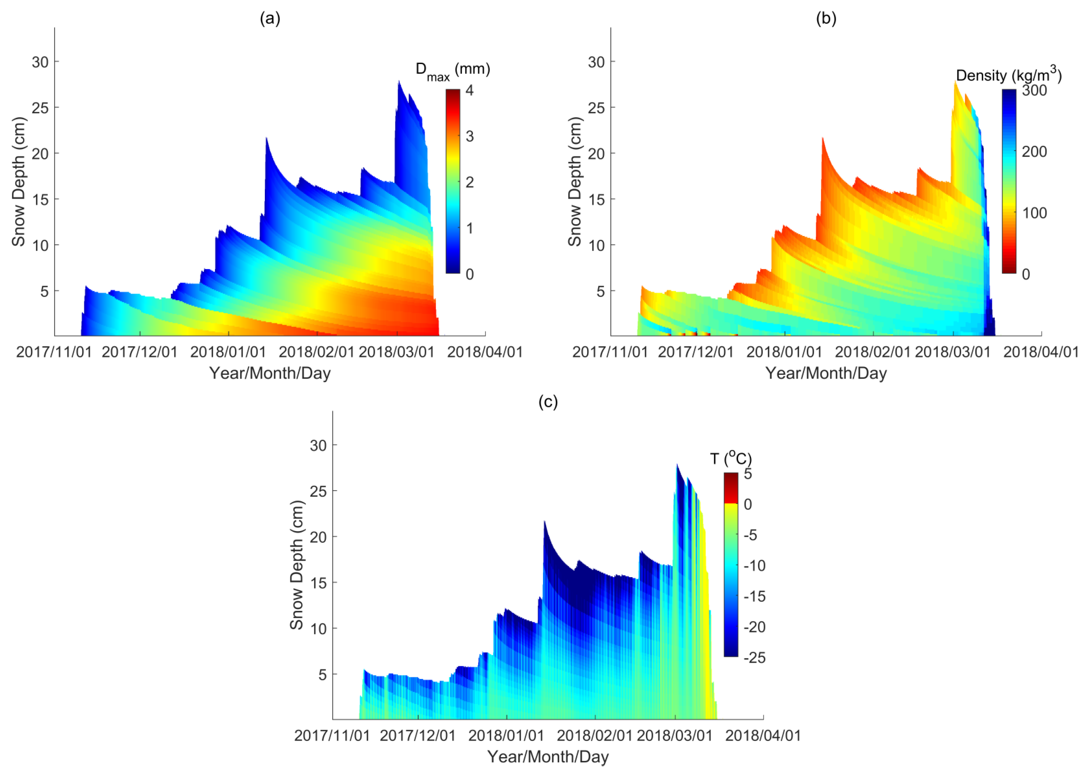
The Altay winter snow observation experiment conducted at the Altay Meteorological Station (47°44′26.58″ N, 88°4′21.55″ E) in Xinjiang, China, from October 2017 to March 2018 provided time series measurements of snowpits and brightness temperature observed by the ground-based radiometer. Chen et al. (2020) [32] used the hourly meteorological forcing data observed at the station (including near-surface air temperature, air pressure, precipitation, wind speed, relative humidity, and solar radiation) to drive SNTHERM and obtained simulated snow profiles at the 1 hour step as shown in Figure 1.

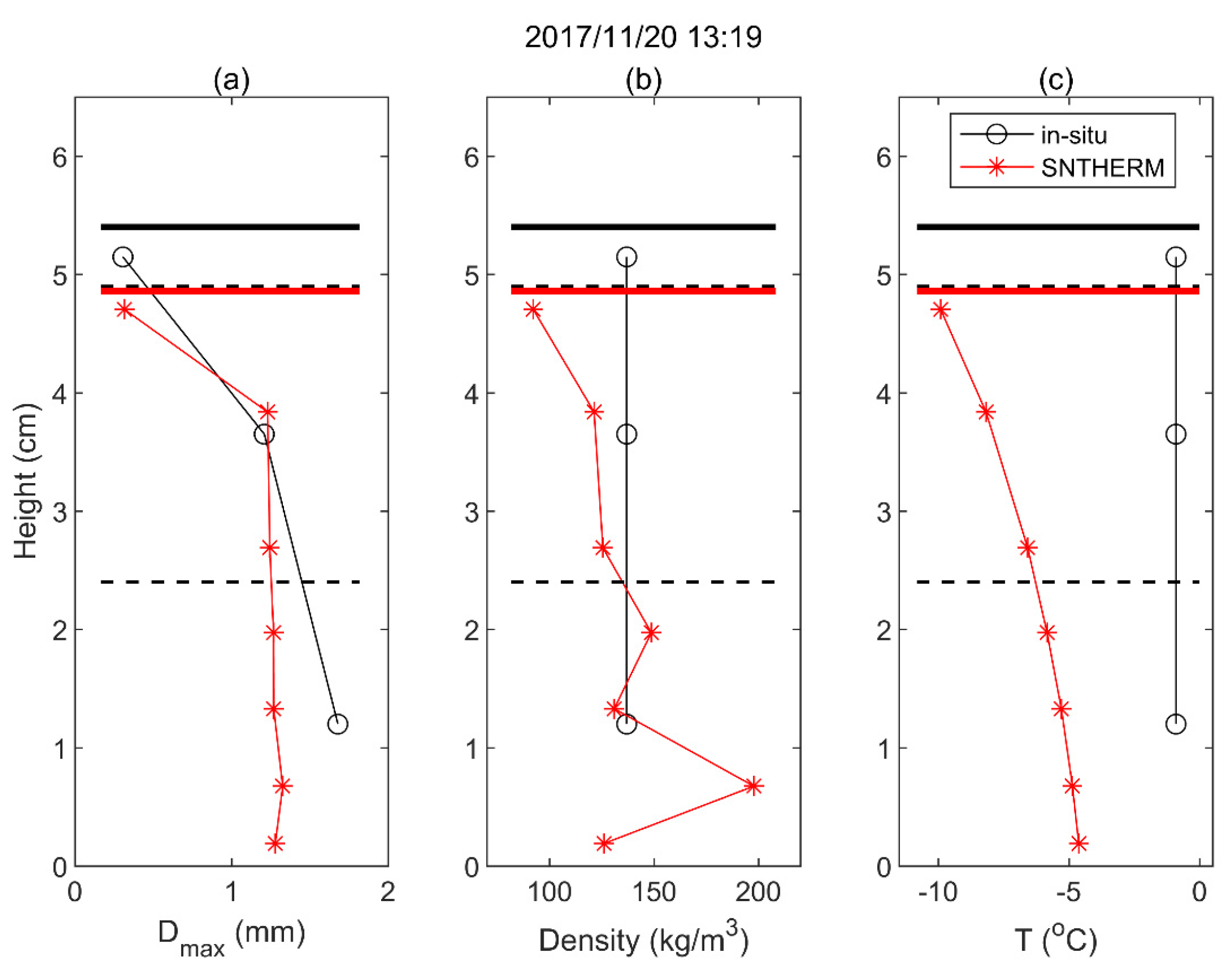
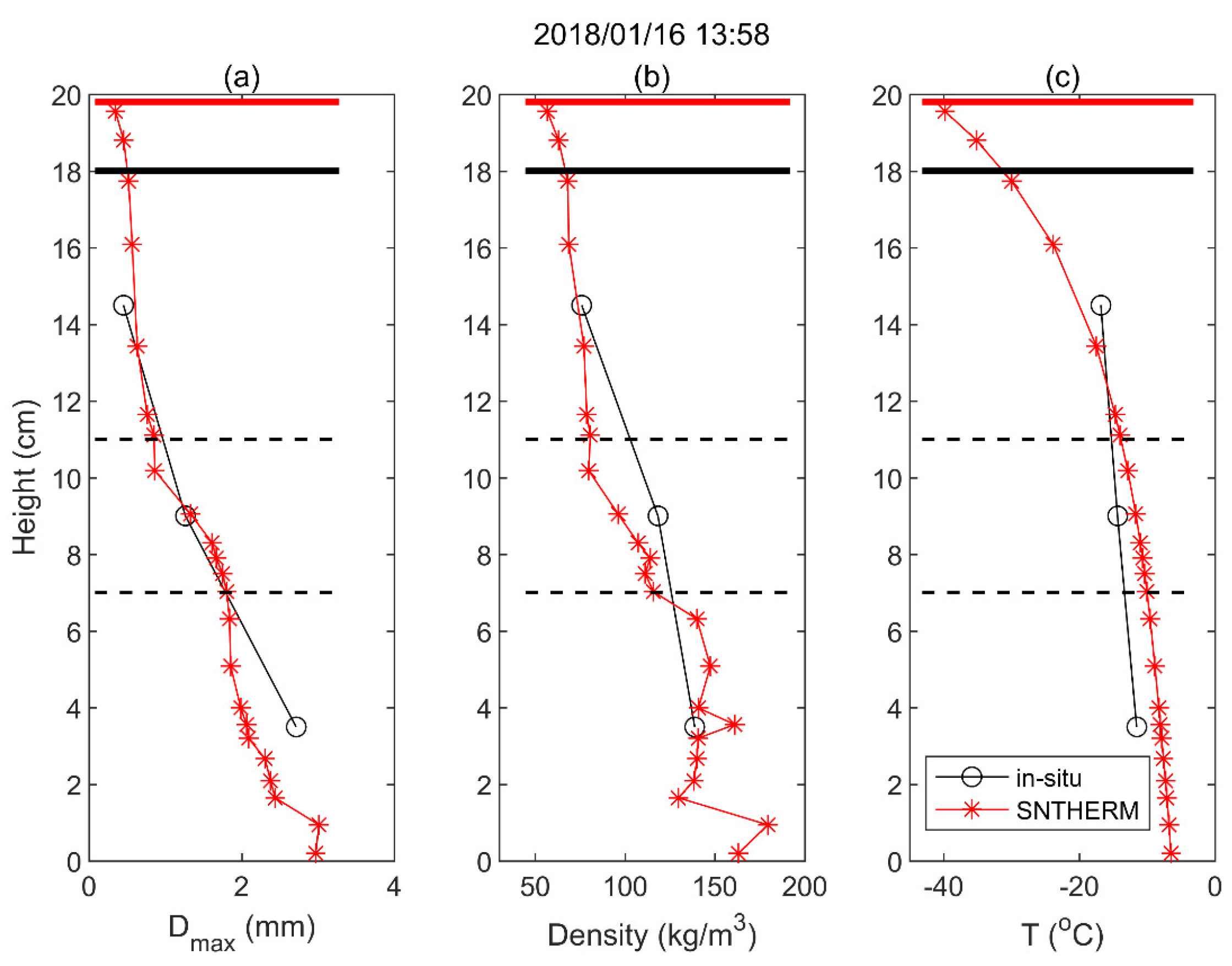
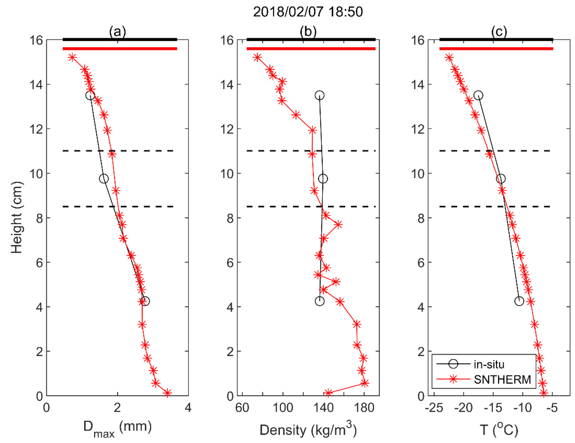
This dataset was used as the samples inputted into MEMLS to study the bulk T_B calculation method. It is composed of 2800 snow profiles with a number of snow layers from 1 to 30, a maximum snow depth up to 28 cm and an average depth of 11.9 cm; more details are summarized in

Table 1. Statistics for the multiple-layer snow properties of the Altay snow samples.

Statistics	Depth (cm)	Layers	Average Density (kg/m3)	Average Geometric Grain Size (mm)	Average Exponential Correlation Length (mm)
Mean	11.9	17	131.54	1.83	0.29
Standard deviation	6.4	10	12.94	0.42	0.04
Maximum	28.0	35	161.64	2.54	0.34
Minimum	2.5	2	93.63	0.25	0.05

. Each sample is a layered snow profile over bare soil that contains the thickness, temperature, density, and SNTHERM-simulated grain size of each snow layer, and the temperature, water content, and unfrozen soil water content averaged over 0–5 cm of soil. The SNTHERM simulated snow depth, layered geometric grain size (D_max), snow density and snow temperature were validated using in situ snowpit measurements in [32]. In Figure 2, Figure 3 and Figure 4, we further present a comparison of vertical profiles on three different days. It shows that SNTHERM captured the vertical variability of the natural snowpack and can provide a finer snow stratigraphic resolution compared to in situ measurements.

2.1.2. Global SNTHERM Simulated Multiple-Layer Snow Dataset

Although the Altay dataset was validated using in situ snow pit observations, this dataset covers only a small range of physical properties constrained by meteorological conditions. Instead of artificially generating random snow property values, we were more interested in a dataset that follows natural snow’s characteristics. Therefore, we conducted a global-scale SNTHERM simulation for application in this study. The SNTHERM was applied to the GLDAS (Global Land Data Assimilation System) meteorological forcing data [34] from August 2016 to August 2017 at a 3 hour step and 0.25° spatial resolution. The SNTHERM adds a new snow layer when snowfall occurs. It also subdivides thick layers to maintain the simulation resolution and accuracy. Therefore, in the standalone SNTHERM code, the number of snow layers allowed is unlimited. To generate the global dataset, the standalone SNTHERM was run uninterrupted. However, after the SNTHERM was running finished, layers more than ten were combined before being saved to the global grids. Layers were combined iteratively by finding the pair of adjacent snow layers with maximum similarity in D_max and density.

In this paper, we selected a longitudinal stripe at 5°–85° N, 90°–95° E in the Northern Hemisphere. The data are from the simulations on 28 February 2017 at 0:00 UTC time. The number of samples was approximately 2500. It covered a large spatial range and different climate zones and, thus, potentially contained a wider range of snow properties compared to the Altay dataset. In Figure 5, a south-to-north profile of D_max and snow density centered at 92.375° E is presented. From the statistics in

Table 2. Statistics of multiple-layer snow properties of global samples in 5°–85° N and 90°–95° E grids.

Statistic	Depth (cm)	Layers	Average Density (kg/m3)	Average Geometric Grain Size (mm)	Average Exponential Correlation Length (mm)
Mean	81.8	10	220.13	1.351	0.248
Standard deviation	34.1	0	32.92	0.334	0.035
Maximum	134.7	10	563.70	2.605	0.344
Minimum	4.1	10	102.32	0.796	0.183

, the maximum snow depth of this dataset can reach 1.3 m, and the average snow depth is 81.8 cm. The number of snow layers was 10 for all samples, because it had reached mid to peak snow season.

2.2. Methods

2.2.1. Snow Brightness Temperature Simulation Models

The MEMLS, based on the improved Born approximation (IBA), was selected as the radiative transfer model to calculate the T_B of multiple-layer and single-layer snowpacks. It calculates the volume scattering of each snow layer using the IBA theory and solves the radiative transfer equation using the six-stream approximation.

The MEMLS model assumes that the snow cover is composed of a set of plane-parallel horizontal layers (j = 1, 2, …, n). At each layer, it uses four fluxes to describe the upward and downward propagated radiations near the upper and lower interfaces, respectively. The fluxes across the interfaces are linked by the Fresnel equation with an assumption that interface bistatic scattering is negligible, and the fluxes inside each layer are linked by the radiative transfer theory. For example, the upward radiation just below the upper interface is composed of the upwelling radiation from the lower interface attenuated by a snow layer transmissivity of t, the downwelling radiation from the upper interface reflected by an internal reflectivity of snow layer r and the thermal emission of the snow layer, denoted by e*T, where e = 1 − r − t, and T is the snow physical temperature. See Equations (1)–(4) and Figure 1 and Figure 2 in [24] for more details. The downwelling sky T_B and the upwelling soil emitted T_B are considered the boundary conditions at the air–snow and snow–soil boundaries, respectively. All these relationships can be used to build a large matrix. The four fluxes at each layer can be solved, and the values at the topmost layer can be used to calculate the T_B observed from the snow’s surface.

In this paper, MEMLS was also used to calculate the scattering coefficient and the internal transmissivity of snow layers to support a standalone calculation of the effective snow microstructure parameter, which is the effective exponential correlation length (p_ex), to be specific. p_ex is a coefficient used to fit the snow autocorrelation function A(x) as A(x) = exp(−x/p_ex). A(x) describes the statistics of correlation between two random points in the snow medium, and x is their distance. The dry snow is composed of ice and air. A(x) is higher if more pairs of points are both occupied by the same component, and lower if one is occupied by ice and the other is occupied by air. The geometric grain size (D_max) simulated by SNTHERM is converted to p_ex following Pan et al. (2016) [19] as:

$$P_{ex}=0.227+0.126\ast \ln D_{max}$$

(1)

where both D_max and p_ex is in mm.

The upwelling soil-emitted T_B was calculated as the product of soil temperature (T_soil) and one minus the snow–soil boundary reflectivity S_ss. S_ss was calculated using the fitted frequency-independent Q-H model in [35], which uses the root mean squared height of the soil surface (rms) as the soil roughness parameter. T_soil and unfrozen soil water content (mv_soil) from the SNTHERM simulations were used to calculate the soil dielectric constants using Zhang et al.’s (2003) model [36]. The rms was set the same as the simulation in Chen et al.’s [32] at Altay, which was 2 cm. Fixed values of downwelling sky T_B (0 K) and rms (2 cm) were used to reduce the influence of nuisance parameters, when the MEMLS multiple-layer snow T_B was compared only with the MEMLS bulk snow T_B. The sky T_B was calculated using air temperature, relative humidity and a standard atmosphere, as described in [37], when the simulation was compared with the T_B observations.

2.2.2. Methods to Calculate the Effective p_ex and Snow Bulk T_B

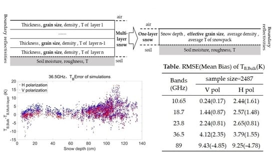
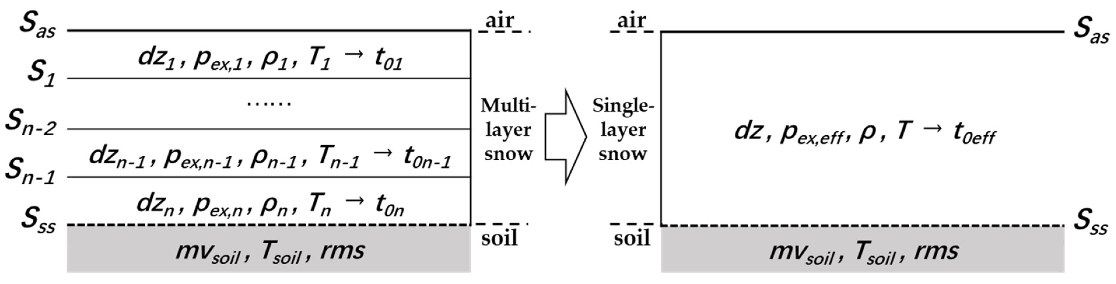
Figure 6 shows the concept of using the snow parameters of a single-layer snowpack to represent the emission of a multiple-layer snowpack. Here, d_z, p_ex, ρ and T are snow thickness, exponential correlation length, density and temperature of each snow layer. The effective p_ex was specially denoted as p_{ex_eff}. S_as and S_ss are the reflectivity of air–snow and snow–soil boundaries, and S₁ to S_n−1 refer to the reflectivity of interfaces between snow layers. t₀₁, t₀₂…t_0n are the one-way transmissivity of each snow layer, and t_0eff is the effective single-layer value.

In MEMLS, the air–snow boundary reflectivity and the interface reflectivity were calculated by the Fresnel equation, with snow permittivity calculated by an empirical model as a function of snow density and temperature in [24]. S_ss is also influenced by the snow density of the bottommost layer. S_ss is important, because the soil emission background is the main source of radiation before it was attenuated by the snow cover. As the snow depth increases, the attenuation increases and, thus, the T_B observed from the snow’s surface decreases. S_as is important because the relative permittivity of air and snow determines the radiation that can pass through the boundary and emit out of the snowpack.

t₀ is an intermediate radiometric parameter defined in [24]. It describes the fraction of radiation attenuated when it propagates through a snow layer once. In [24], it is officially called the one-way transmissivity. t₀ is calculated as:

$$t_0=\exp \left(-\gamma \ast dz\ast \sec \theta \right)$$

(2)

where dz is the layer thickness. $\theta$ is the local incidence angle of microwave inside this layer. $dz\ast \sec \theta$ is also called the slant thickness. $\gamma$ is the damping coefficient calculated as:

$$\gamma =\sqrt{{\gamma }_a^{\prime }\left({\gamma }_a^{\prime }+2{\gamma }_b^{\prime }\right)}$$

(3)

Here, ${\gamma }_a^{\prime }$ and ${\gamma }_b^{\prime }$ are the two-flux equivalent absorption and scattering coefficients in the backward direction, calculated from the six-flux absorption coefficient (${\gamma }_{\mathrm{a}}$) and scattering coefficient (${\gamma }_b$ in backward direction and ${\gamma }_c$ in horizontal direction). ${\gamma }_{\mathrm{a}}$, ${\gamma }_b$ and ${\gamma }_c$ are directly calculated by the IBA as a function of snow density, p_ex and temperature [25]. ${\gamma }_{\mathrm{a}}$ is mainly determined by snow density, whereas ${\gamma }_b$ and ${\gamma }_c$ are mainly determined by p_ex. For dry snow, the scattering effect is usually much larger than the absorption/re-emission effect. Therefore, p_ex is the key parameter for the snow volume scattering.

It can be seen from the physical theory in MEMLS that the snow density mainly determines the soil background radiation emitted across the snow–soil boundary, and p_ex mainly influences the snow medium’s attenuation from the volume scattering. When T_B at the snow’s surface decreases with snow depth, it acts like the intercept (at zero depth, unit: K) and slope (unit: 1/cm), respectively, as in the parameterized model described in Jiang et al. (2007) [38]. Therefore, our formulation of a bulk T_B calculation method considers both the boundary condition and p_ex. Also, as presented in many previous studies [24,25,26,27], the relationship between the p_ex and scattering coefficient is nonlinear. Larger snow particles produce much larger scattering. Therefore, compared to a mass-weighted average p_ex that is mass conversative in the snow physics, a new effective p_ex that is radiative conversative in snow emission theory needs to be formulated.

In the following subsections, four different methods to calculate the effective p_ex and bulk T_B are described. In all of the methods, the single-layer snow thickness is the summed thickness of all the layers (i.e., snow depth), and the single-layer snow temperature is the mass-weighted average snow temperature of all the layers (T_avg).

(1)

Option 1: Use the mass-weighted average p_ex of the multiple layers (p_ex,avg) as the effective p_ex to calculate the snow scattering coefficient and use the mass-weighted average density (ρ_avg) to calculate S_as and S_ss. See Equations (4)–(6). This is the simplest and most mass conservative method without consideration of any nonlinearity in snow radiative transfer theory.

$$p_{ex,avg}=\frac{{{\displaystyle \sum }}_{i=1}^n{W}_i·p_{ex,i}}{{{\displaystyle \sum }}_{i=1}^n{W}_i}$$

(4)

$${\rho }_{avg}=\frac{{{\displaystyle \sum }}_{i=1}^n{W}_i·{\rho }_i}{{{\displaystyle \sum }}_{i=1}^n{W}_i}$$

(5)

where n is the total number of snow layers, and,

$$W_i={\rho }_i\ast d{z}_i$$

(6)

(2)

Option 2: Use the product of one-way transmissivity of all layers as the effective one-way transmissivity (t0eff) and retrieve pex,eff according to t0eff using a look-up table generated using MEMLS-IBA (see Equations (7)–(10)). Use ρavg to calculate Sas and Sss.

$$t_{0eff}=t_{01}\ast t_{02}\dots \ast t_{0j}$$

(7)

$$t_{0eff}=\exp \left(-{\gamma }_{eff}\ast d{z}^{\prime }\right)$$

(8)

where

$$d{z}^{\prime }={\displaystyle \sum }_{i=1}^{n}d{z}_i\ast sec{\theta }_i$$

(9)

$${\gamma }_{eff}=M_{IBA}\left(p_{ex,eff},T_{avg},{\rho }_{avg}\right)$$

(10)

Here, ${\gamma }_{eff}$ is the effective damping coefficient. M_IBA represents the look-up table generated by MEMLS-IBA.

(3)

Option 3: Calculate pex,eff using the same method in Option 2, but use the density of the topmost and bottommost snow layer to calculate Sas and Sss.

(4)

Option 4: Use pex,avg to calculate the snow scattering coefficient. Use the density of the topmost and bottommost snow layer to calculate Sas and Sss.

In general, Option 3 is the most complicated method. Option 4 features a simplification in effective p_ex, to be compared with Option 3.

When the T_B of a multiple-layer snowpack is regarded as the true value, the brightness temperature error (T_B Error) of the bulk T_B calculated by these four methods (T_B,bulk) is calculated as:

$$T_{B}Error=T_{B,bulk}-T_{B,true}$$

(11)

The root mean square error (RMSE) is calculated as:

$$RMSE=\sqrt{\frac{{{\displaystyle \sum }}_{i=1}^N{\left(T_B{}_{i,bulk}-T_B{}_{i,true}\right)}^2}{N}}$$

(12)

where N is the number of samples.

The correlation coefficient R between T_B,bulk and T_B,true is calculated as:

$$R=\frac{{{\displaystyle \sum }}_{i=1}^N\left(T_{B_{i,bulk}}-\overline{T_{B_{bulk}}}\right)\left(T_{B_{i,true}}-\overline{T_{B_{true}}}\right)}{\sqrt{{{\displaystyle \sum }}_{i=1}^N{\left(T_{B_{i,bulk}}-\overline{T_{B_{bulk}}}\right)}^2\ast {{\displaystyle \sum }}_{i=1}^N{\left(T_{B_{i,true}}-\overline{T_{B_{true}}}\right)}^2}}$$

(13)

2.2.3. Fitted Effective p_ex to Match the multiple-layer Brightness Temperature

Another common way to find the effective p_ex is to iteratively tune and fit this parameter until it matches the multiple-layer T_B. A difference with the previous studies is that we used the same S_as and S_ss as the multiple-layer snowpack calculated from the topmost and bottommost snow density as in Option 2 and 3. The cost function is:

$$\mathrm{F}\left(p_{ex,fit}\right)=T_{B,MEMLS}\left(freq, pol,\theta , p_{ex,fit}\left({\rho }_{avg}\right),SD,T_{avg},S_{as},S_{ss}\right)-T_{B,MEMLS}\left(freq, pol,\theta , p_{ex,i~n},d_{z,i~n},T_{i~n},{\rho }_{i~n}\right)$$

(14)

where freq and pol stand for the frequency and polarization, respectively. SD is the snow depth. p_ex,fit is the fitted p_ex to be calculated.

The iteration started from the mass-weighted p_ex,avg and stopped until the cost function was smaller than 0.1 K. The relationship between p_ex,avg, p_ex,eff and p_ex,eff was studied.

2.2.4. Effective p_ex with the Consideration of Penetration Depth

At high frequencies, there is the possibility that the microwave cannot propagate through the entire snowpack. In other words, the bottom layers become “in-observable” by the radiometer. The emission from these layers cannot reach the snow’s surface, and the T_B from the snow’s surface loses the sensitivity to their snow properties.

Therefore, here, the concept of penetration depth is introduced to constrain the snow layers involved in bulk T_B calculation in surface layers. Penetration depth refers to the depth at which the electromagnetic wave can penetrate. It is determined both by the medium properties and the microwave wavelength. The distance at which the intensity is attenuated to 1/e (e ≈ 2.77) of its original value is a commonly used cut-off threshold. In this study, the powers of 1/e were tested, too. With the penetration depth considered, the new $t_{0eff}^{\prime }$ and ${\gamma }_{eff}^{\prime }$was recalculated using Equation (15) and used to retrieve effective p_ex using Equation (10).

$t_{0eff}^{\prime }$ is defined as:

$$t_{0eff}^{\prime }=\exp \left(-{\gamma }_{eff}^{\prime }\ast d{z}^{″}\right)={\displaystyle \prod }_{i=1}^m{t}_{0i}\approx CR=1/e^k$$

(15)

where

$$d{z}^{″}={\displaystyle \sum }_{i=1}^{m}d{z}_i\ast sec{\theta }_i$$

(16)

where m ≤ n. k is changed in order to find m, and afterwards, m is used to calculate $t_{0eff}^{\prime }$. $T_{avg}$ and ${\rho }_{avg}$ used to find $p_{ex,eff}$ using the M_IBA look-up table were also calculated from layer 1 to m.

3. Results

3.1. Comparison of Four Bulk T_B Calculation Methods

3.1.1. Results Based on the Altay Snow Samples

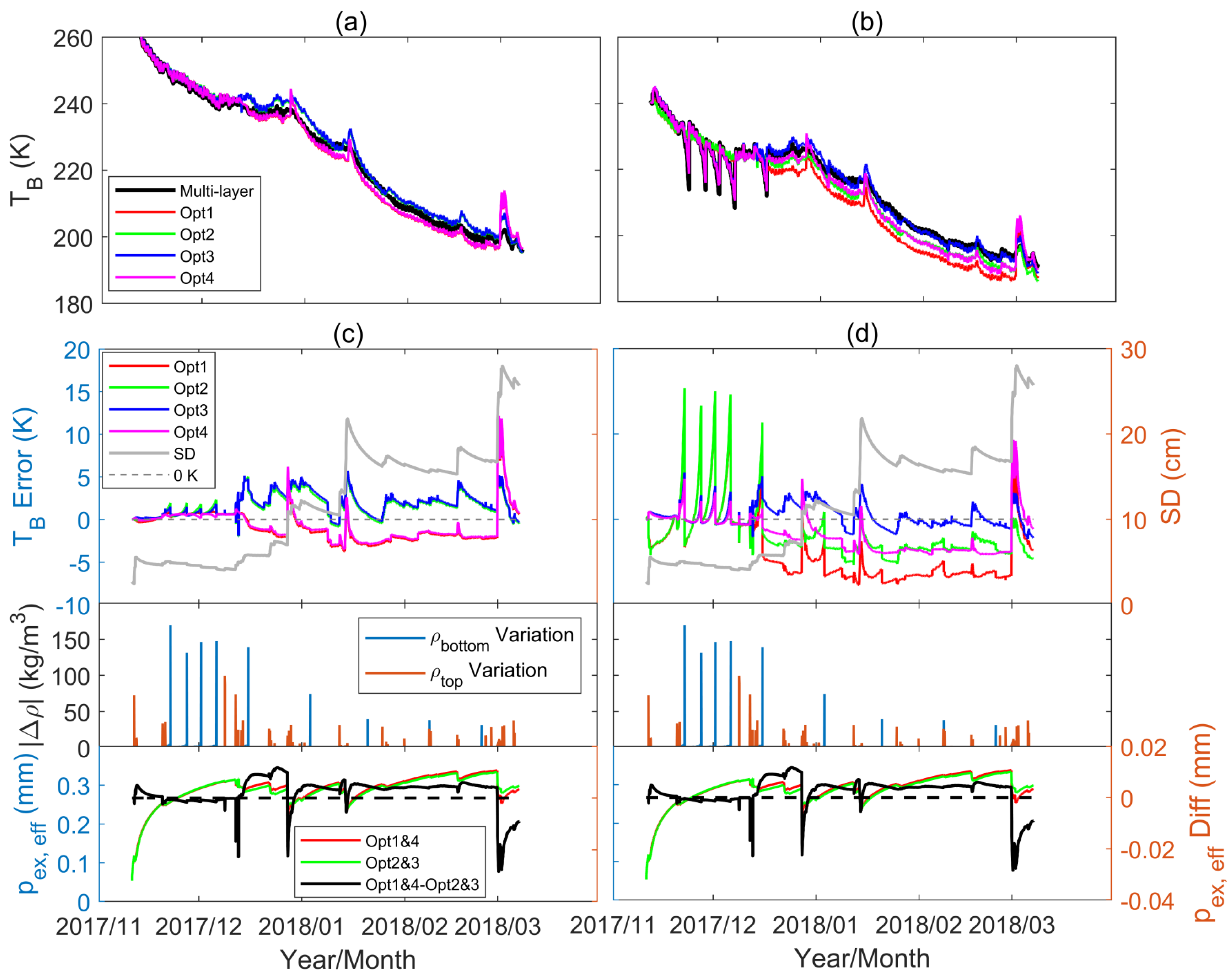
First, the four methods to calculate the effective p_ex and the corresponding bulk T_B described in Section 2.2.2 were evaluated using the multiple-layer snow samples from the Altay experiment at an incidence angle of 55° and at the frequencies of 10.65 GHz, 18.7 GHz, 23.8 GHz, 36.5 GHz and 89 GHz. The simulated brightness temperature at 36.5 GHz and the T_B Error are shown in Figure 7. The x-axis is time. In order to improve the understanding of T_B Error, the snow depth is presented in thick gray lines. The change in snow density at the topmost and bottommost layers between two adjacent samples in a time series, calculated as $\left|\Delta \rho \right|=\left|{\rho }_i-{\rho }_{i-1}\right|$, are represented as orange and blue lines, respectively, where i is the sample ID. The results at other frequencies are shown in Figure 8.

As can be seen in Figure 7, at 36.5 GHz, in most cases, the absolute value of T_B Error is smaller than 5 K at both polarizations, which is approximated at 2.3% relative error (5 K divided by 220 K). Five kelvins is between the observation accuracy of the radiometer (2–3 K) and the accuracy of snow radiative transfer models (10–15 K) [18,19,29,30,31,32,39]. Two factors lead to the difference of T_B error calculated by different options. One was from the abrupt change in the local snow density near the air–snow and snow–soil boundaries. The change in the topmost snow density was from the new snowfall. The change in the bottommost snow density was basically due to the arithmetic in the snow process model calculation. Although the snow density of a single layer in most cases monotonically increases due to the snow compaction [24], when the sublimation and windblown effects at the snow’s surface are excluded, the mass of the bottommost snow layer can decrease due to the movement of water vapor to upper layers. At some point, the mass of the bottom layer decreases to zero and is combined with the adjacent layer in the next step. At this turning point, an abrupt change in the bottommost snow density occurred, because we updated the snow density in a timely manner. It can be seen in Figure 7d that using the mass-weighted average snow density of the entire snowpack (Options 1 and 2) will result in an overestimation of T_B observed at the snow’s surface, up to ~15 K. However, using the local density near the air–snow and snow–soil boundaries, in other words, to keep the same boundary reflectivity as the multiple-layer snow case, will largely reduce the T_B Error to ~5 K. From a comparison between Figure 7c,d and Figure 8, it shows the importance of boundary reflectivity, as it was much stronger at low frequencies and horizontal polarization. This led to a generally smaller RMSE at vertical polarization than horizontal polarization. The second was from the single-layer exponential correlation length used for simulation. The same p_ex,avg was used for both polarizations, same as for p_ex,eff. At 36.5 GHz, vertical polarization, when the p_ex,avg used in Options 1 and 4 was larger than p_ex,eff used in Options 2 and 3 at approximately 0.005 mm, it resulted in a smaller bulk T_B, ~4 K on average. Note that the influence of p_ex was so large because the absolute value of p_ex was large after November 2017. In Figure 7c, it also shows that the difference from the different boundary reflectivities was very small at 36.5 GHz, vertical polarization. However, at the horizontal polarization in Figure 7d, the T_B difference from the boundary reflectivity was of the same magnitude (~4 K) as the difference from the p_ex. In Figure 7d, Option 1 gave the largest mean bias, whereas Option 3 gave the smallest mean bias; these two methods had differences in both the boundary reflectivity and effective p_ex choices.

Another interesting point in Figure 7c,d is that after January 2018, the variation in the T_B Error sometimes showed a short-time local correlation with the variation in snow depth. This is because the Altay samples were from a continuous snow process. At each time step, the snow compaction and snow grain growth resulted in a continuous change in thickness, density, and grain size of each layer, and these parameters further influenced the local interface reflectivity and scattering coefficient. In a simplified single-layer model, it is indeed impossible to capture all the fine resolution details inside the snowpack. Therefore, a drift of T_B Error due to the combined effect is understandable. Such phenomenon is only found at a short time scale. For all the samples, the T_B error and snow depth are clearly uncorrelated.

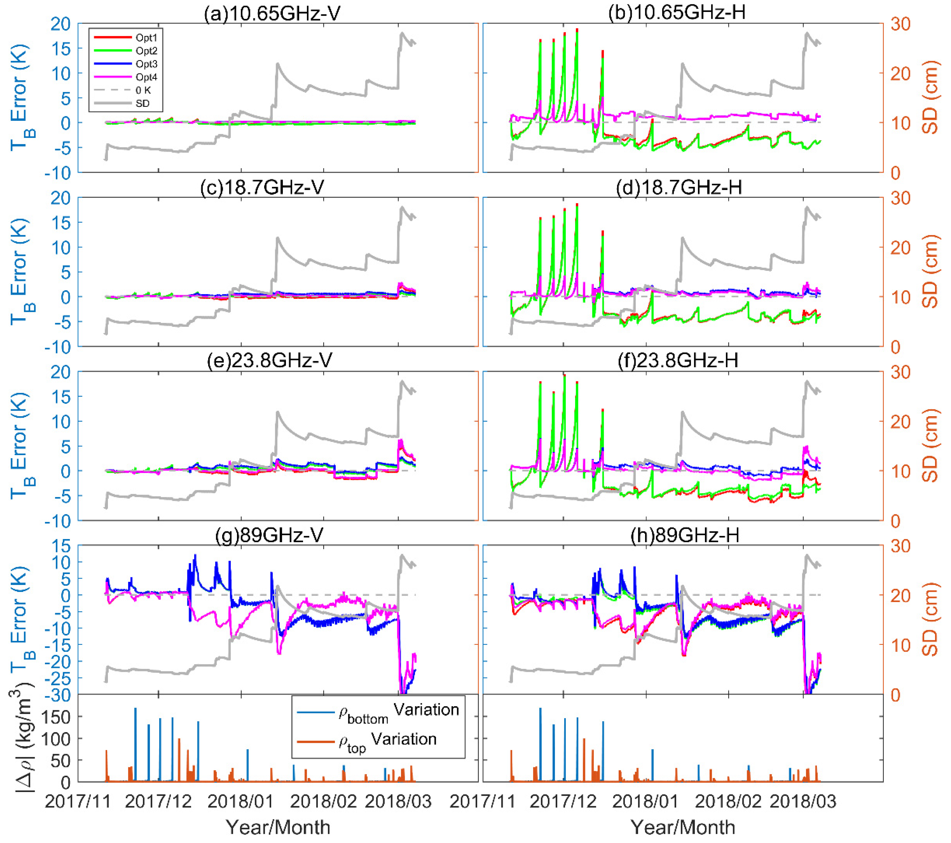
In general, the result at 36.5 GHz shows that Option 3 is the best effective p_ex and bulk T_B calculation method. Later, we explored the results at other frequencies (see Figure 8). Figure 8 shows clearly that at 10.65 to 23.8 GHz, the use of boundary reflectivity calculated by local snow density (Options 3 and 4) gave less biased simulation at horizontal polarization. A comparison between Options 3 and 4 shows that, the difference from different p_ex was less than 1 K. From the statistics of mean bias, RMSE, and correlation coefficient in

Table 3. Statistics for mean bias (MB), RMSE, and correlation coefficient (R) of simulated brightness temperature in different bands and polarizations (Altay samples). The sample size was 3016. The values in bold represent the highest accuracy among four methods.

Frequency (GHz)	Polarization	MB(K)				RMSE (K)				R
		Opt1	Opt2	Opt3	Opt4	Opt1	Opt2	Opt3	Opt4	Opt1	Opt2	Opt3	Opt4
10.65	H	−1.96	−2.20	1.51	1.51	4.11	4.26	1.31	1.31	0.332	0.335	0.984	0.985
18.7	H	−2.51	−2.63	0.88	0.78	4.25	4.29	0.99	0.91	0.097	0.119	0.983	0.981
23.8	H	−2.73	−2.59	0.68	0.35	4.61	4.34	1.06	1.22	0.559	0.585	0.975	0.953
36.5	H	−3.85	−2.23	0.18	−1.63	5.40	3.50	1.39	2.77	0.973	0.983	0.996	0.992
89	H	−6.74	−6.32	−5.89	−6.14	8.57	8.57	8.38	8.16	0.968	0.969	0.969	0.969
10.65	V	−0.24	−0.30	0.11	0.10	0.28	0.29	0.09	0.08	0.981	0.982	0.999	0.999
18.7	V	−0.07	0.01	0.36	0.22	0.43	0.28	0.48	0.48	0.981	0.996	0.995	0.981
23.8	V	−0.12	0.26	0.57	0.14	1.11	0.75	0.95	1.13	0.979	0.994	0.993	0.978
36.5	V	−0.87	1.23	1.43	−0.72	2.18	2.10	2.06	2.10	0.995	0.998	0.997	0.995
89	V	−5.41	−4.88	−4.86	−5.39	7.91	8.38	8.37	7.90	0.970	0.968	0.968	0.970

, it shows Option 4 had the best performance at 10.65 and 18.7 GHz, whereas Option 3 had a smaller RMSE and higher correlation coefficient at 23.8 and 36.5GHz. The performance at 89 GHz was quite different with other frequencies. In Figure 8g–h, from mid-November 2017 to January 2018, the simulation using p_ex,eff (Options 2 and 3) gave a smaller bias; however, after mid-January 2018, the simulation using p_ex,avg (Options 1 and 4) gave a smaller bias. The influence of boundary reflectivity was minor at both polarizations. The performance of different options was unstable. From the statistics, it showed the RMSE at 89 GHz at both polarizations can reach 8 K, which is at least three times of other frequencies.

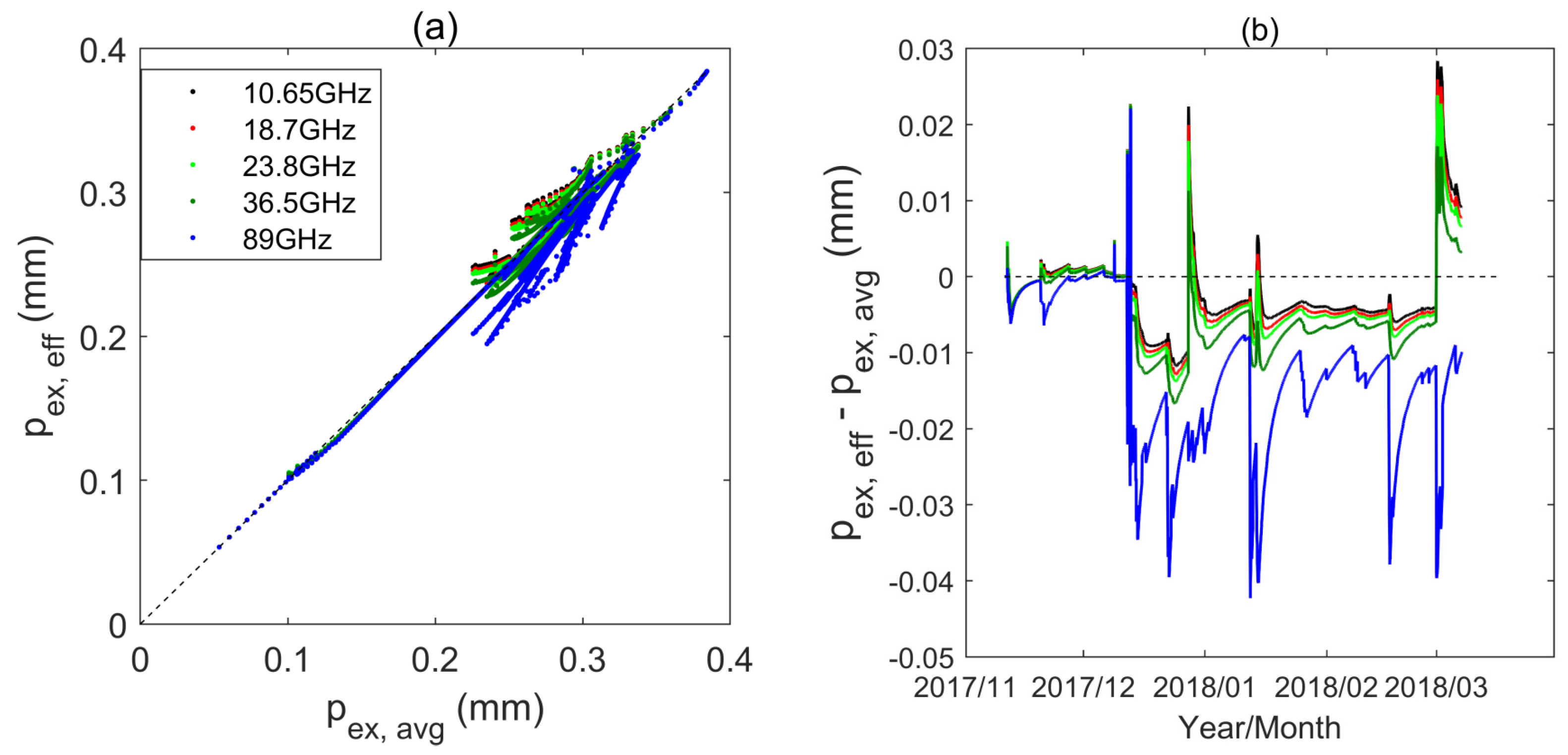
Figure 9 shows a comparison of p_ex,eff at different frequencies. It shows this parameter was smaller at higher frequencies. This was because the smaller penetration depth at high frequencies gives larger weight to surface snow layers.

3.1.2. Results Based on the Global Snow Process Model Simulation Samples

In this section, the global simulated snow samples from a longitudinal stripe described in Section 2.1.2 were used to evaluate the T_B Error of four methods at an incidence angle of 55°. The statistics of the mean bias (MB), RMSE, and R are listed in

Table 4. Statistics for mean bias (MB), RMSE and correlation coefficient (R) of simulated brightness temperature in different bands and polarizations (global samples). The sample size was 2487. The values in bold represent the highest accuracy among four methods.

Frequency (GHz)	Polarization	MB(K)				RMSE(K)				R
		Opt1	Opt2	Opt3	Opt4	Opt1	Opt2	Opt3	Opt4	Opt1	Opt2	Opt3	Opt4
10.65	H	−8.03	−8.15	1.62	1.61	8.67	8.79	2.46	2.44	0.718	0.715	0.919	0.920
18.7	H	−6.76	−6.35	1.98	1.48	7.41	6.91	2.73	2.57	0.784	0.831	0.930	0.914
23.8	H	−5.91	−4.71	2.08	0.81	6.69	5.29	2.92	2.65	0.894	0.934	0.955	0.927
36.5	H	−8.72	−6.90	−3.75	−5.14	9.20	7.93	5.58	5.76	0.974	0.954	0.950	0.980
89	H	−27.95	−36.87	−36.50	−26.29	32.09	39.97	39.64	30.61	0.698	0.709	0.704	0.688
10.65	V	−0.80	−0.82	0.21	0.17	0.98	1.03	0.27	0.24	0.987	0.985	0.999	0.999
18.7	V	0.19	0.79	1.54	0.87	1.15	1.14	1.73	1.44	0.979	0.990	0.994	0.981
23.8	V	0.36	1.84	2.38	0.81	2.08	2.36	2.80	2.24	0.974	0.987	0.988	0.973
36.5	V	−5.16	−3.48	−3.31	−5.05	5.94	5.76	5.69	5.86	0.984	0.959	0.958	0.983
89	V	−26.71	−36.96	−36.95	−26.69	31.14	40.21	40.20	31.12	0.686	0.690	0.690	0.686

, and the comparison of p_ex,eff, p_ex,avg, and p_ex,fit is presented in Figure 10.

Table 4 shows that, like the results from Altay samples, the T_B Error at the vertical polarization was smaller than the horizontal polarization, and the T_B RMSE from the best model at each frequency from 10.65 to 36.5 GHz was no larger than 6 K. However, none of the four methods was applicable to 89 GHz, where the T_B error RMSE was at least 30 K. At horizontal polarization, the performance of using the correct boundary reflectivity (Options 3 and 4) was better than the other choice. Between Option 3 and Option 4, similar to the results from the Altay samples, Option 4 performed better at 10.65 and 18.7 GHz, and Option 3 was better at 36.5 GHz. The difference in the results from the global samples shows Option 4 also performed better at 23.8 GHz.

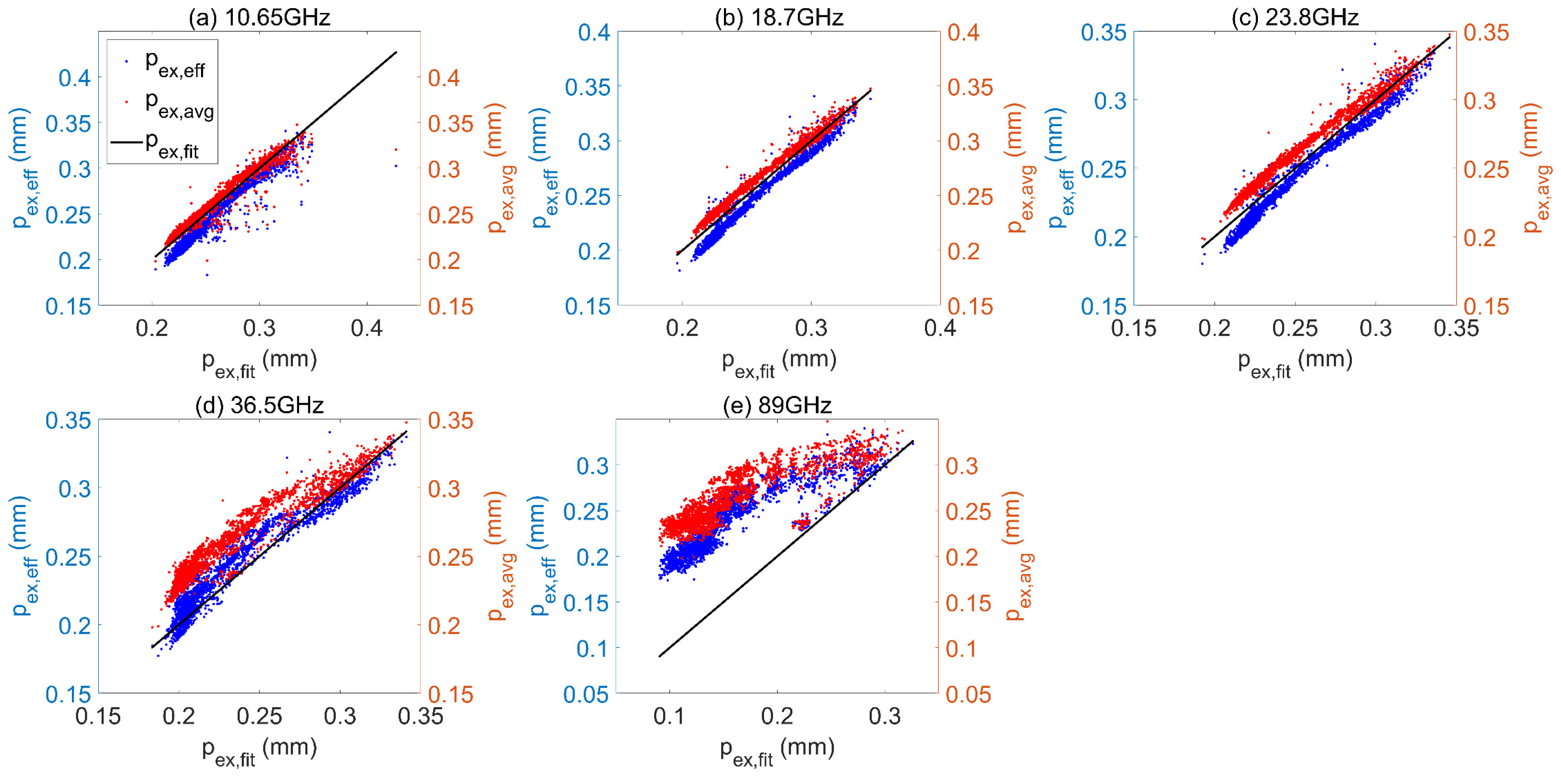
Figure 10 shows a comparison between p_ex,eff and p_ex,avg using the global snow samples. p_ex,fit can be considered as the true value, as it was fitted to match the multiple-layer T_B. In all cases, p_ex,eff was larger than p_ex,avg. At 10.65 to 23.8 GHz, both p_ex,eff and p_ex,avg were close to p_ex,fit, whereas p_ex,eff showed an underestimation and p_ex,avg showed an overestimation. p_ex,eff was unbiased at 36.5 GHz. At 89GHz, both p_ex,avg and p_ex,eff were strongly overestimated, especially for the small grain size cases.

3.2. Sensitivity Analysis of Bulk T_B Error

This section explores the sensitivity of T_B Error to the incident angle, snow mass-weighted average grain size, and snow depth using Option 3 and the global snow samples.

3.2.1. Sensitivity of T_B Error to Incident Angle

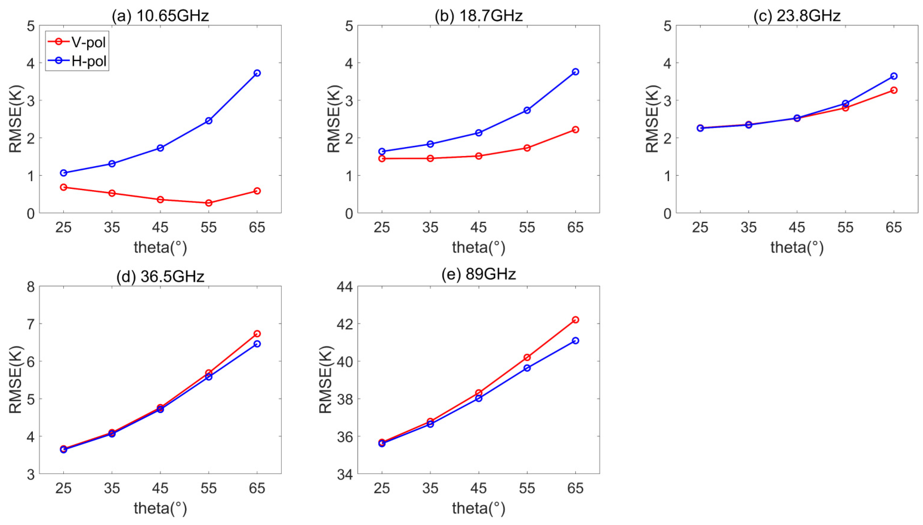
Figure 11 shows the sensitivity of T_B Error to incidence angle at different frequencies. It shows that T_B Error generally increases with the incidence angle (except at 10.65 GHz, horizontal polarization), because the slant snow depth ($SD\ast \sec \theta$) increases with $\theta$. However, as the incidence angle increases from 25° to 65°, the increase in T_B RMSE was smaller than 3 K. At all angles, T_B RMSE was smaller than 4 K at 10.65 to 23.8 GHz, and smaller than 7 K at 36.5 GHz.

Figure 11 also shows the sensitivity of the T_B RMSE at the horizontal polarization was larger than vertical polarization at low frequencies (10.65 and 18.7 GHz), but it was smaller at high frequencies (36.5 and 89 GHz). This indicates that the boundary reflectivity dominated the performance at low frequencies, whereas the accuracy of effective p_ex and volume scattering calculation was more important at high frequencies. At 89 GHz, T_B RMSE increased from ~35 K at 25° to ~41 K at a 65° incidence angle.

3.2.2. Sensitivity of T_B Error to Average p_ex

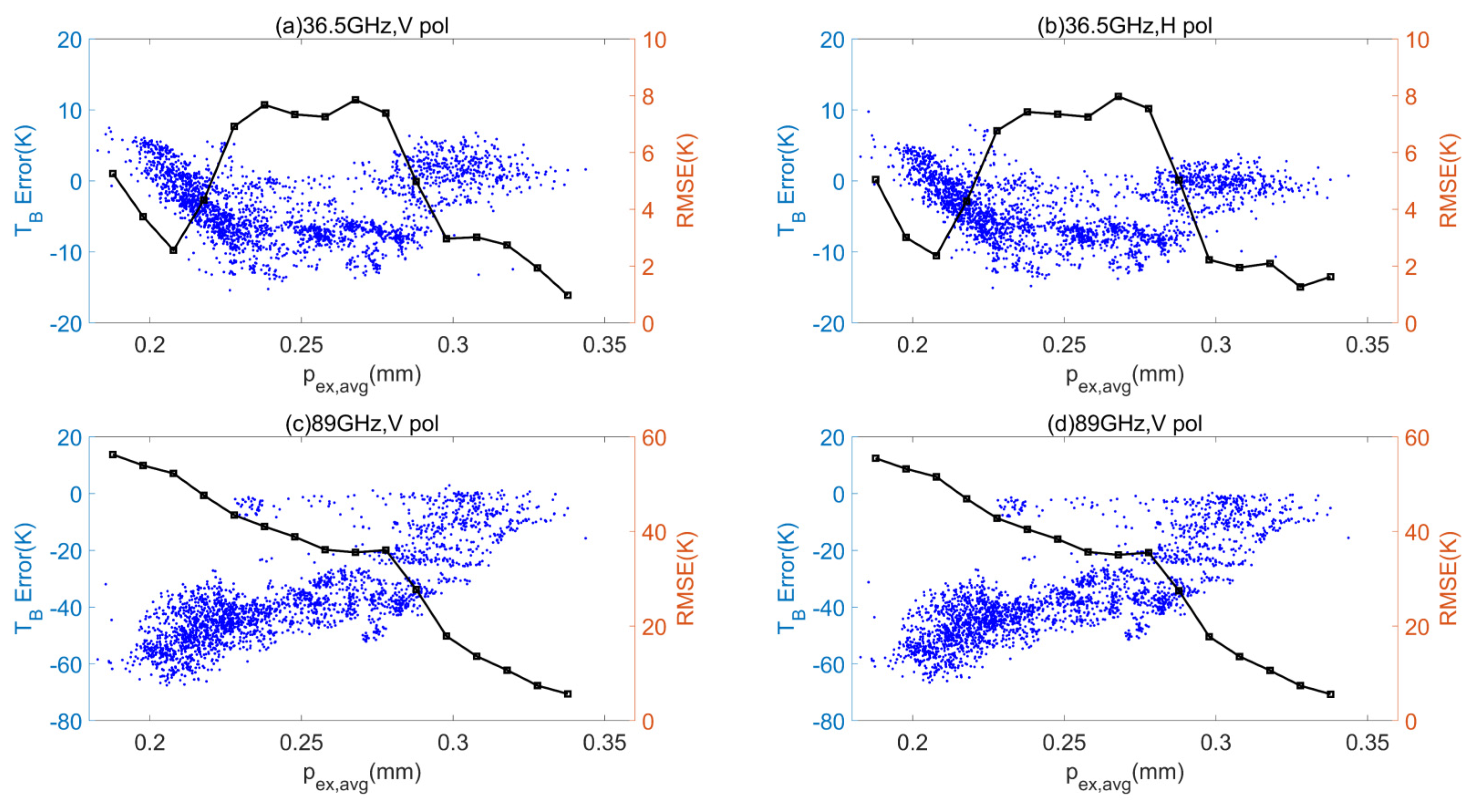
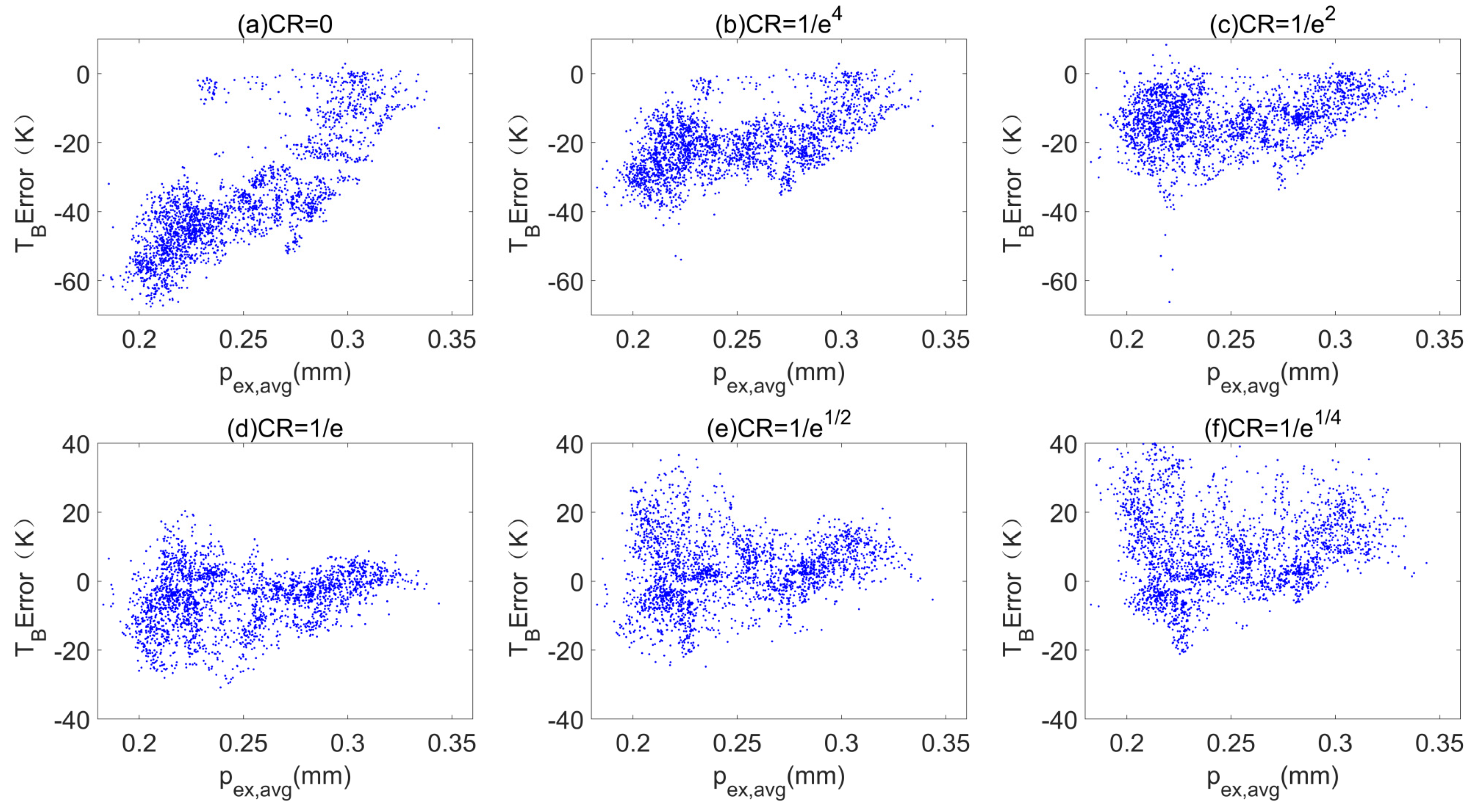
Figure 12 shows the sensitivity of T_B Error to p_ex,avg, which represents the average level of snow particle sizes. Only the results at 36.5 and 89 GHz are presented, because the volume scattering is less important at lower frequencies. The incidence angle was 55°. Figure 12 shows T_B RMSE at 36.5 GHz was the largest at medium values of p_ex,avg. However, in general, it was uncorrelated with p_ex,avg. At 89 GHz, T_B Error distribution gave a relatively complex pattern. The scatter points can be summarized in two groups. In the first group, the bulk T_B was unbiased and generally insensitive to p_ex,avg (see the points of T_B Error > –5 K). In the second group, the bulk T_B was significantly underestimated, and the underestimation decreased as p_ex,avg increased. This indicates the strongly underestimated T_B at 89 GHz came from the small grain size samples. It does not mean the influence of p_ex to T_B is smaller for small p_ex, but is more likely related to the characteristics of natural snow—p_ex,avg is smaller for deeper snowpacks. The results in Section 3.2.3 prove this assumption. The results at other incidence angles were similar.

3.2.3. Sensitivity of T_B Error to Snow Depth

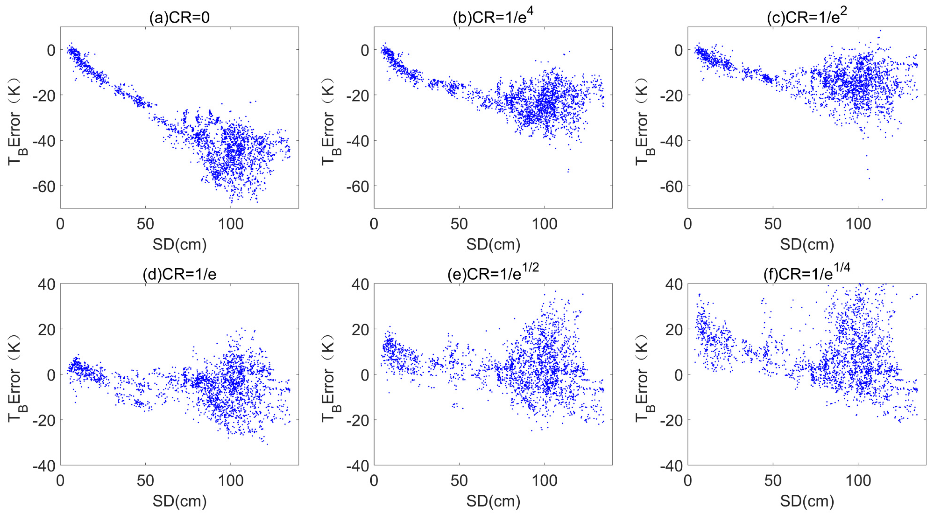
Figure 13 shows the sensitivity of T_B Error to snow depth. It shows in all cases that the T_B RMSE was larger for thicker snow, expect at 10.65 GHz. This is understandable. From 10.65 to 36.5 GHz, the T_B Error and snow depth was uncorrelated, although some samples tended to be overestimated for thick snow from 10.65 to 23.8 GHz and underestimated at 36.5 GHz. Only at 89 GHz was the underestimation of T_B and the snow depth highly correlated. When snow depth reached 1 meter, the bulk T_B could be underestimated by 60 K compared to the multiple-layer T_B.

3.3. Improvement of Bulk T_B at High Frequencies Using the Penetration Depth

In this section, the concept of penetration depth was applied to improve the bulk T_B performance at 36.5 and 89 GHz.

At 89 GHz, the underestimation of bulk T_B and snow depth was highly correlated. Here, by reducing the range of snow layers involved in p_ex calculation to surface layers using different cut-off thresholds (i.e., CR values), the accuracy of the simulated T_B at 89 GHz was significantly improved (

Table 5. Statistics for mean bias (MB), RMSE, and correlation coefficient (R) with different penetration depth thresholds (CR) at 89 GHz and a 55° incidence angle. The values in bold represent the highest accuracy among different CR thresholds.

CR	V pol.			H pol.
	MB (K)	RMSE (K)	R	MB (K)	RMSE (K)	R
0	−36.95	40.20	0.690	−36.50	39.64	0.704
1/e4	−20.42	22.08	0.930	−20.14	21.72	0.933
1/e2	−13.32	15.36	0.927	−13.13	15.08	0.929
1/e	−4.85	9.43	0.919	−4.78	9.25	0.920
1/e1/2	3.38	10.23	0.898	3.28	9.97	0.901
1/e1/4	8.83	15.13	0.861	8.56	14.63	0.867

). When the CR value gradually increased from 0 to 1/e, the T_B RMSE decreased from 40.20 to 9.43 K at vertical polarization, whereas that at horizontal polarization was reduced from 39.64 to 9.25 K. The accuracy was the highest when CR=1/e and started to decrease when CR further increased to 1/e^1/4. It can clearly be seen in Figure 14 and Figure 15 that the underestimation for deep snow and small p_ex,avg was reduced when the CR value gradually increased from 0 to 1/e^1/2. However, a very large value of CR at 1/e^1/4 led to an overestimation of T_B. Therefore, the best CR threshold was near 1/e, where the T_B RMSE at both polarizations could be reduced to below 10 K at 89 GHz.

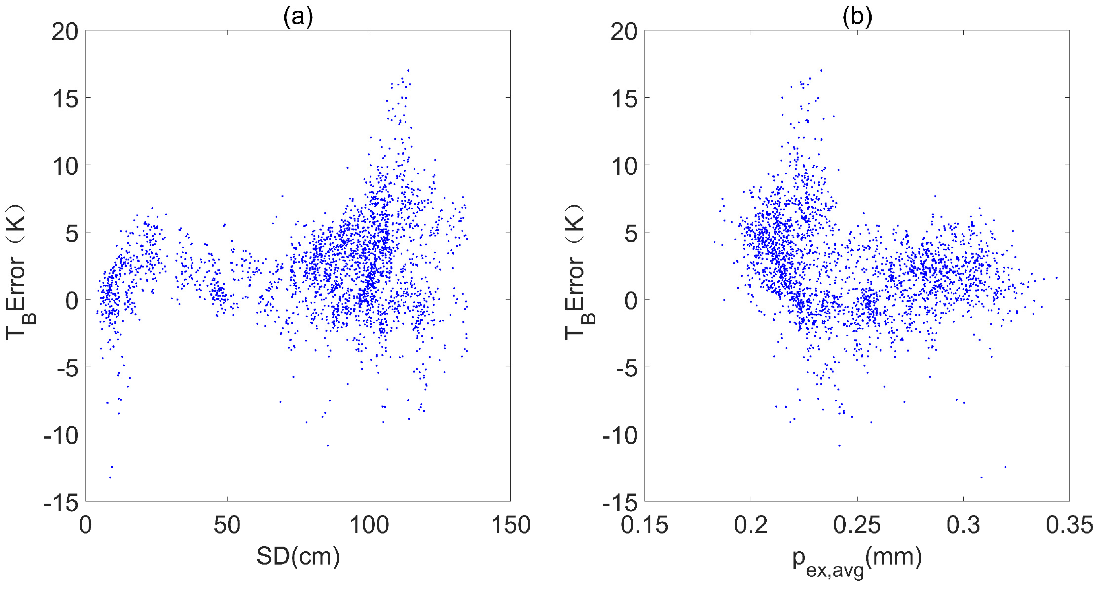
At 36.5 GHz, the bulk T_B was underestimated for some thick snow (>60 cm) and medium p_ex,avg (approximately 0.25 mm) cases. Here, the results in

Table 6. Statistics for mean bias (MB), RMSE and correlation coefficient (R) with different penetration depth thresholds (CR) at 36.5 GHz and a 55° incidence angle. The values in bold represent the highest accuracy among different CR thresholds.

CR	V pol.			H pol.
	MB (K)	RMSE (K)	R	MB (K)	RMSE (K)	R
0	−3.31	5.69	0.958	−3.75	5.58	0.950
1/e4	−3.31	5.69	0.958	−3.75	5.58	0.950
1/e2	−3.30	5.66	0.959	−3.73	5.55	0.950
1/e	2.35	4.12	0.970	1.55	3.79	0.954
1/e1/2	14.59	16.59	0.825	12.77	14.92	0.754
1/e1/4	23.00	25.41	0.656	20.24	22.59	0.573

and Figure 16 show that the use of a cut-off threshold of 1/e for the product of transmissivity improved the accuracy of these samples and reduced the overall RMSE from approximately 5.6 to about 4 K.

3.4. Application of the Optimal Method

3.4.1. Application to In-Situ Snow Profile and Ground-Based Radiometer Measurements

Summarizing Section 3.1, Section 3.2 and Section 3.3, the optimal method for calculating bulk T_B is to use p_ex,avg, S_as, and S_ss calculated from the local density near the boundaries for 10.65 to 23.8 GHz, and use p_ex,eff calculated from the product of one-way transmissivity of snow layers within the penetration depth of microwaves propagating from the snow’s surface and S_as and S_ss calculated from the local density near the boundaries at 36.5 and 89 GHz.

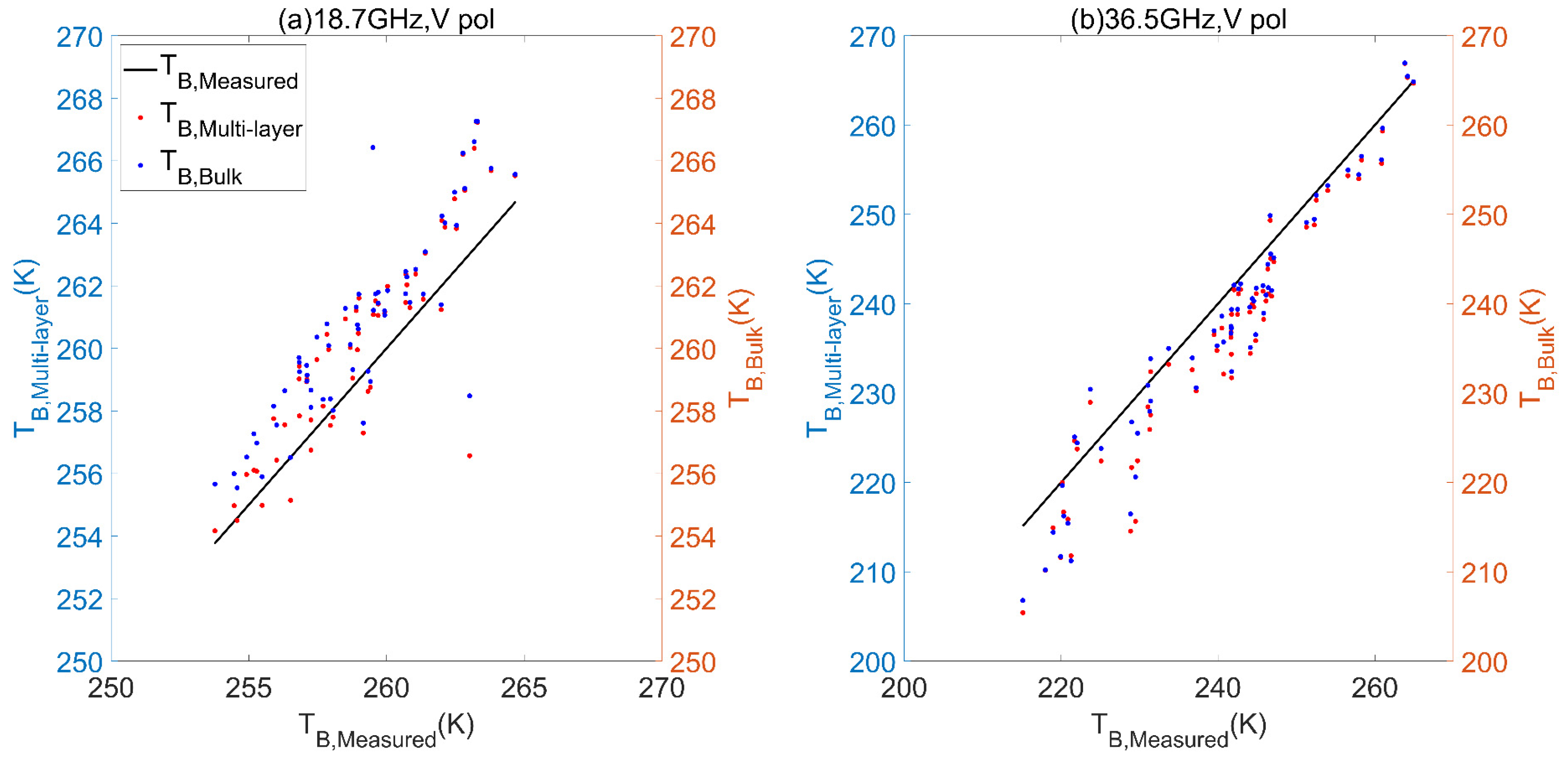
The optimal methods were applied to the in situ snow profile measurements from the Altay experiment. The bulk T_B was compared with the T_B measured by a ground-based radiometer (see Chen et al. (2020) [32]), and the error from single-layer approximation was compared to the model error of MEMLS.

Table 7. Error statistics for the MEMLS-simulated multiple-layer brightness temperature (T_{B,Multi-layer}), MEMLS-simulated single-layer temperature (T_B,Bulk) and brightness temperature measured by ground-based radiometer (T_B,Measured).

Error (K)	RMSE (MB) (Sample Size = 63)
	18.7 V	18.7 H	36.5 V	36.5 H
TB,Multi-layer − TB,Measured	2.08(1.22)	6.91(6.29)	5.53(−4.01)	5.84(−4.13)
TB,Bulk − TB,Measured	2.20(1.64)	7.10(6.51)	4.74(−3.11)	6.44(−4.72)
TB,Bulk − TB,Multi-layer	0.63(0.43)	0.42(0.23)	1.41(0.90)	1.16(−0.59)

Note that, compared to the result in [32], the measured single-layer snowpits were not included in the statistics of T_{B,Multi-layer} − T_B,Measured.

and Figure 17 show that the MEMLS model error was between 2–7 K, whereas the error of single-layer approximation itself was only between 0.6–1.5 K. The error of single-layer approximation applied for in situ snowpits was even smaller than that applied for SNTHERM-simulated profiles in Table 3, because the observed snow profiles had much fewer layers.

3.4.2. Comparison to Satellite T_B and the Problems

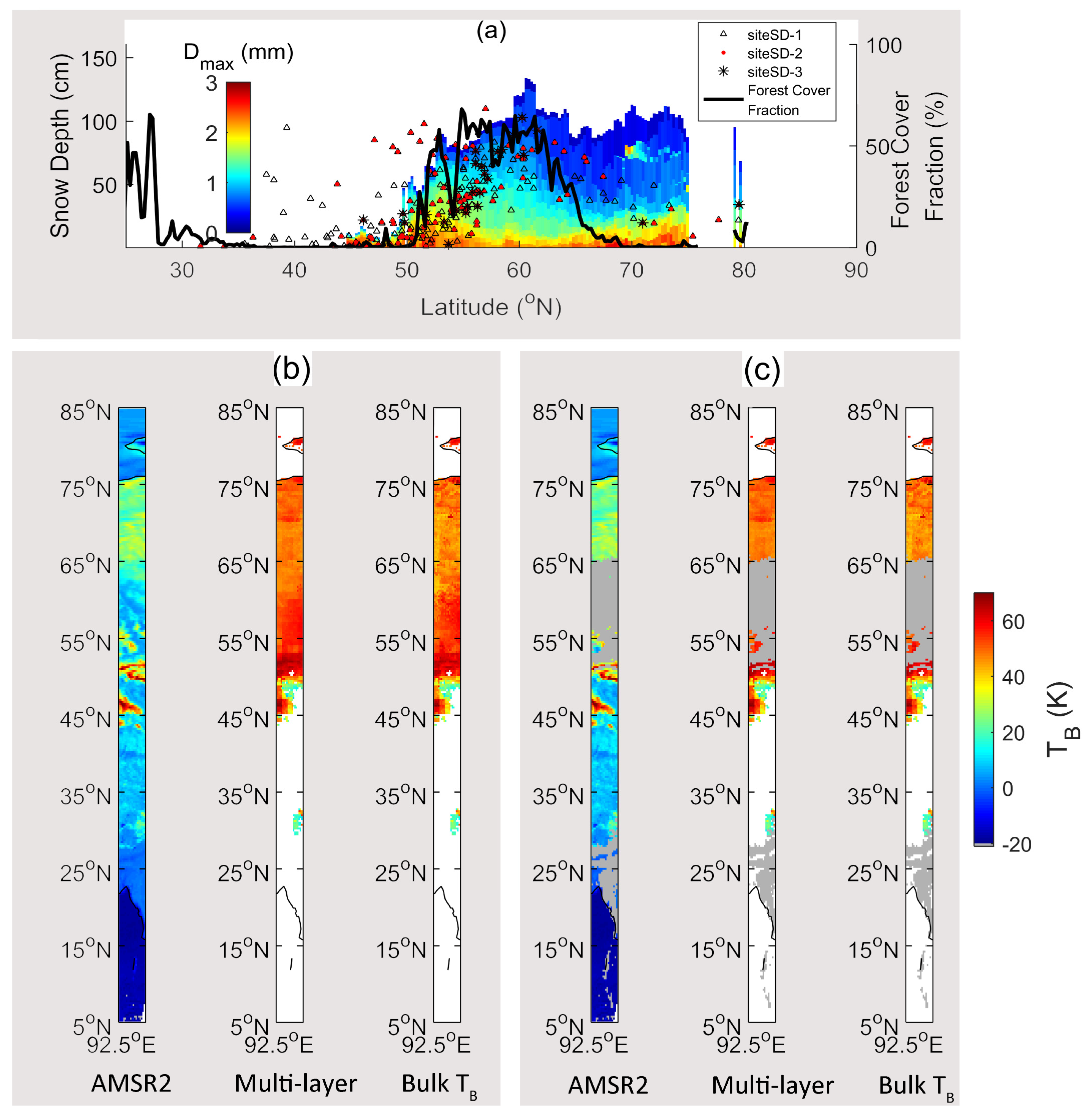
In this section, the MEMLS-simulated 18.7–36.5 GHz T_B difference using multiple and single snow profiles for vertical polarization, calculated in Section 3.1.2, are presented as a geographic map in Figure 18b. It shows that the MEMLS simulations in these two cases had a similar spatial distribution pattern.

The satellite-observed T_B from the Advanced Microwave Scanning Radiometer 2 (AMSR2) [40] is also presented. The daily snow depth measurements from the meteorological stations in the Global Historical Climatology Network [41,42], and the forest cover fraction of a 0.25° spatial resolution calculated from the MODIS/Terra Vegetation Continuous Fields Yearly L3 Global 250 m SIN Grid Version 6 (MOD44B v006) dataset [43] were introduced in the error analysis.

It can be seen from Figure 18b, c that the simulated T_B was different with the AMSR2 T_B north of 52° N. The reasons are as follows.

First, it can be seen in Figure 18a that GLDAS+SNTHERM simulated the snow depth measured at the meteorological stations north of 65° N more than once. Because there are only two stations within the 90–95 ° E range (see black asteroids), measurements from stations in a wider longitude range (70–115 °E) are also presented (see black triangles and red points). Because of the overestimation of snow depth, the simulated snowpack gave stronger volume scattering, which resulted in an overestimation of the 18.7–36.5 GHz T_B difference, north of 65 ° N. The average AMSR2 T_B difference was approximately 30 K, whereas the GLDAS+SNTHERM+MEMLS simulation reached approximately 50 K. The overestimation of the SNTHERM-simulated snow depth was not because SNTHERM did not contain a canopy interception module for the snowfall, because the forest fraction was below 20% north of 65° N. More work is needed to check the error in the GLDAS forcing data and the deficiency of SNTHERM. SNTHERM also does not consider the windblown effect; however, it is unlikely half of the snow was blown off by wind.

Second, between 52° and 65° N, the forest cover fraction was larger than 20%. The forest canopy can strongly attenuate the volume scattering signal emitted from the snow’s surface. As a result, the 18.7–36.5 GHz T_B difference will decrease. The modelling tool used in this study has only a snow emission model; the forest emission model is not included. Therefore, the T_B difference in 52′65° N was also overestimated, which was approximately 50–60 K compared to 10–20 K observed by AMSR2.

4. Discussion

In this paper, a method for calculating a single-layer effective microstructure parameter that can reproduce the T_B of a multiple-layer natural snowpack was formulated. The proposed single-layer approximation method was mainly established based on the physical radiative transfer theory and through a model-to-model comparison study based on MEMLS. Compared to previous studies [12,13,14], the effective microstructure parameter was not fitted from any real T_B observations. No observation error or radiative transfer model error were involved in the evaluation of the optimal method.

In previous studies, the focus was not on finding the theory of how a multiple-layer snowpack can be radiometrically equivalent to a single-layer snowpack. An effective microstructure parameter was fitted from T_B observations. The focus was on the possibility of simultaneously conducting effective grain size and snow water equivalent (SWE) retrievals [12], proving the existence of a consistent effective grain size fitted from the ground-based, airborne, and satellite T_B observations using the same snow emission model [13] and the relationship between the effective grain sizes fitted from radiometer and radar and, consequently, the possibility to use the former as prior knowledge for radar SWE retrieval [14].

Because the effective microstructure parameter was completely fitted from T_B observations using a cost function between the model simulation and observations [12,13,14], the importance of keeping the multiple-layer snow case boundary conditions was not found.

In [12], Kongoli et al. (2008) generated a look-up table by one-layer DMRT snow emission model (range of inputs: 1–60 cm snow depth, 0.25–0.75 mm snow grain radius) and used this table to simultaneously find the snow depth and grain radius of the closest match to the atmosphere corrected land surface emissivity. He only empirically considered the influence of penetration depth at high frequencies, by tuning the one-layer snow grain radius to 0.8, 0.6, and 0.5 of the low-frequency values at 50, 89, and 157 GHz, respectively. When the retrieval method was applied in the Continental US on April 15, 2008, the forest influence was not considered.

In Lemmetyinen et al. (2015) [13], the effective grain size was fitted from tower-based, mobile sled-based, airborne and satellite T_B near Sodankylä, Finland, based on cost functions. The snow emission model was the Helsinki University of Technology (HUT) model. Concurrent field experiments were carried out to provide information about snow depth and snow vertical properties for the effective grain size fitting. It was found that the use of at least two snow layers can improve the simulation accuracy for mobile sled-based T_B and for airborne T_B for snowpits in forests and over lakes at 36.5 GHz. The multiple-layer configuration was not important for airborne-level simulation at 18.7 GHz. This was consistent with our study. Lemmetyinen et al. (2015) proved that the effective grain size and the measured average geometric grain size have relationships that vary temporally. Because their T_B modelling tool incorporated a forest and an atmosphere correction model, they successfully retrieved very close effective grain size of a similar seasonal variation trend from the ground-based, airborne and satellite T_B observations. The modelling tool used in our study failed to do so (Section 3.4.2), but our main conclusion was unaffected. In [13], it was pointed out that the fitted grain size contains errors unrelated to the effective snow grain size from vegetation, soil conditions, scene heterogeneity, etc.

In [14], the effective p_ex was fitted based on MEMLS3&a [44] using the tower-based passive microwave and active microwave observations. It was found that the effective p_ex fitted from 18.7–37 GHz T_B difference for vertical polarization was highly correlated with that fitted from 10.2–16.7 GHz VV backscattering coefficient difference (in dB), although their absolute values were different.

In this paper, the SNTHERM simulated snow depth driven by GLDAS did not fully match the observed snow depth in the global snow samples; the satellite T_B cannot be reproduced because of the error in simulated snow depth and the lack of forest T_B correction model. These factors led to some differences between the global snow samples and the actual conditions. Our study was based on MEMLS. Therefore, although it has considered the physical theory, the main conclusions may still need to be re-evaluated if other snow emission models are used.

5. Conclusions

This paper described our study of the method of using single-layer snow parameters to reproduce the T_B of multiple-layer snowpacks based on MEMLS model simulations and natural snow’s characteristics. The results showed that it is important to use the same air–snow and snow–soil boundary reflectivity as the multiple-layer snow case, which can largely improve the accuracy of bulk T_B compared to multiple-layer T_B at low frequencies and for horizontal polarization. After the correct boundary reflectivity is used, the simple mass-weighted average snow p_ex can be used for 10.65 to 23.8 GHz. For higher frequencies, it is suggested to use the product of one-way snow layer transmissivity within the microwave penetration to retrieve the effective p_ex.

The optimal method provided an RMSE of single-layer approximation of less than 5 K for 10.65 to 36.5 GHz, and less than 10 K for 89 GHz. The error was insensitive to incidence angle, average p_ex, and snow depth.

The effective microstructure parameter is widely used in snow water equivalent (SWE) retrieval. The research in this study provides a method for calculating the effective microstructure parameter of a snowpack using only the snow physical parameters, without the need for T_B observations.

References

- Joshua, K.; Chris, D.; Peter, T.; Alexandre, L.; Chris, L.; Juha, L.; Phil, M.; Benoit, M.; Alexandre, R.; Nick, R.; et al. The influence of snow microstructure on dual-frequency radar measurements in a tundra environment. Remote Sens. Environ. 2018, 215, 242–254. [Google Scholar]
- Domine, F.; Albert, M.; Huthwelker, T.; Jacobi, H.W.; Kokhanovsky, A.A.; Lehning, M.; Picard, G.; Simpson, W.R. Snow physics asrelevant to snow photochemistry. Atmos. Chemistryand Phys. 2008, 8, 171–208. [Google Scholar] [CrossRef] [Green Version]
- Dozier, J.; Painter, T.H. Multispectral and hyperspectral remote sensing of alpine snow properties. Ann. Rev. Earth Planet. Sci. 2004, 32, 465–494. [Google Scholar] [CrossRef] [Green Version]
- Grenfell, T.C.; Warren, S.G. Representation of a nonsperical ice particle by a collection of independent spheres for scattering and absorption of radiation. J. Geophys. Res. 1999, 104, 31697–31709. [Google Scholar] [CrossRef]
- Chang, T.C.; Gloersen, P.; Schmugge, T.; Wilheit, T.T.; Zwally, H.J. Microwave emission from snow and glacier ice. J. Glaciol. 1976, 16, 23–39. [Google Scholar] [CrossRef] [Green Version]
- Nolin, A.W.; Dozier, J. A hyperspectral method for remotely sensing the grain size of snow. Remote Sens. Environ. 2000, 74, 207–216. [Google Scholar] [CrossRef]
- Mätzler, C. A simple snow pack/cloud reflectance and teansmittance model from microwave to ultraviolet: The ice-lamella pack. J. Glaciol. 2000, 46, 20–24. [Google Scholar] [CrossRef]
- Mätzler, C. Relation between Grain-Size and Correlation Length of Snow. J. Glaciol. 2002, 48, 461–466. [Google Scholar] [CrossRef] [Green Version]
- Negi, H.S.; Kokhanovsky, A. Retrieval of snow albedo and grain size using reflectance measurements in Himalayan basin. Cryosphere 2011, 5, 203–217. [Google Scholar] [CrossRef] [Green Version]
- Wang, J.G.; Feng, X.Z.; Xiao, P.F.; Ye, N.; Zhang, X.L.; Cheng, Y.Y. Snow grain-size estimation over mountainous areas from MODIS imagery. IEEE Geosci. Remote Sens. Lett. 2017, 15, 1–5. [Google Scholar] [CrossRef]
- Donahue, C.; Skiles, S.M.; Hammonds, K. In situ effective snow grain size mapping using a compact hyperspectral imager. J. Glaciol. 2021, 67, 49–57. [Google Scholar] [CrossRef]
- Kongoli, C.; Boukabara, S.A.; Weng, F. The retrievals of effective grain size and snow water equivalent from variationally-retrieved microwave surface emissivities. In Proceedings of the 2008 Microwave Radiometry and Remote Sensing of the Environment, Florence, Italy, 25 July 2008. [Google Scholar]
- Lemmetyinen, J.; Derksen, C.; Toose, P.; Proksch, M.; Pulliainen, J.; Kontu, A.; Rautiainen, K.; Seppänen, J.; Hallikainen, M. Simulating seasonally and spatially varying snow cover brightness temperature using HUT snow emission model and retrieval of a microwave effective grain size. Remote Sens. Environ. 2015, 156, 71–95. [Google Scholar] [CrossRef]
- Lemmetyinen, J.; Derksen, C.; Rott, H.; Macelloni, G.; King, J.; Schneebeli, M.; Wiesmann, A.; Leppänen, L.; Kontu, A.; Pulliainen, J. Retrieval of effective correlation length and snow water equivalent from radar and passive microwave measurements. Remote Sens. 2018, 10, 170. [Google Scholar] [CrossRef] [Green Version]
- Wiesmann, A.; Mätzler, C.; Weise, T. Radiometric and structural measurements of snow samples. Radio Sci. 1998, 33, 273–289. [Google Scholar] [CrossRef]
- Hallikainen, M.T.; Ulaby, F.T.; Van Deventer, T.E. Extinction behavior of dry snow in the 18-to 90-GHz Range. IEEE Trans. Geosci. Remote Sens. 1987, 25, 737–745. [Google Scholar] [CrossRef]
- Surdyk, S. Using microwave brightness temperature to detect short-term surface air temperature changes in Antarctica: An analytical approach. Remote Sens. Environ. 2002, 80, 256–271. [Google Scholar] [CrossRef]
- Durand, M.; Kim, E.J.; Margulis, S.A. Quantifying uncertainty in modeling snow microwave radiance for a mountain snowpack at the point-scale, including stratigraphic effects. IEEE Trans. Geosci. Remote Sens. 2008, 46, 1753–1767. [Google Scholar] [CrossRef]
- Pan, J.M.; Durand, M.; Sandells, M.; Lemmetyinen, J.; Kim, E.J.; Pulliainen, J.; Kontu, A.; Derksen, C. Differences between the HUT snow emission model and MEMLS and their effects on brightness temperature simulation. IEEE Trans. Geosci. Remote Sens. 2016, 54, 2001–2019. [Google Scholar] [CrossRef]
- Brucker, L.; Picard, G.; Arnaud, L.; Barnola, J.-M.; Schneebeli, M.; Brunjail, H.; Lefebvre, E.; Fily, M. Modeling time series of microwave brightness temperature at Dome C, Antarctica, using vertically resolved snow temperature and microstructure measurements. J. Glaciol. 2011, 57, 171–182. [Google Scholar] [CrossRef] [Green Version]
- Du, J.Y.; Shi, J.C.; Rott, H. Comparison between a Multi-scattering and Multi-layer Snow Scattering Model and its Parameterized Snow Backscattering Model. Remote Sens. Environ. 2010, 114, 1089–1098. [Google Scholar] [CrossRef]
- Takala, M.; Luojus, K.; Pulliainen, J.; Derksen, C.; Lemmetyinen, J.; Kärnä, J.P.; Koskinen, J.; Bojkov, B. Estimating northern hemisphere snow water equivalent for climate research through assimilation of space-borne radiometer data and ground-based measurements. Remote Sens. Environ. 2011, 115, 3517–3529. [Google Scholar] [CrossRef]
- Tedesco, M.; Jeyaratnam, J. A new operational snow retrieval algorithm applied to historical AMSR-E brightness temperatures. Remote Sens. 2016, 8, 1037. [Google Scholar] [CrossRef] [Green Version]
- Mätzler, C.; Wiesmann, A. Microwave emission model of layered snowpack. Remote Sens. Environ. 1999, 70, 307–316. [Google Scholar] [CrossRef]
- Mätzler, C.; Wiesmann, A. Extension of the Microwave Emission Model of Layered Snowpack to Coarse-Grained Snow. Remote Sens. Environ. 1999, 70, 317–325. [Google Scholar] [CrossRef]
- Tsang, L.; Pan, J.; Liang, D.; Li, Z.; Cline, D.W.; Tan, Y. Modeling active microwave remote sensing of snow using dense media radiative transfer (DMRT) theory with multiple-scattering effects. IEEE Trans. Geosci. Remote Sens. 2007, 45, 990–1004. [Google Scholar] [CrossRef]
- Picard, G.; Brucker, L.; Roy, A.; Dupont, F.; Fily, M.; Royer, A.; Harlow, C. Simulation of the microwave emission of multi-layered snowpacks using the Dense Media Radiative transfer theory: The DMRT-ML model. Geosci. Model. Dev. 2013, 6, 1061–1078. [Google Scholar] [CrossRef] [Green Version]
- Löwe, H.; Picard, G. Microwave scattering coefficient of snow in MEMLS and DMRT-ML revisited: The relevance of sticky hard spheres and tomography-based estimates of stickiness. Cryosphere 2015, 9, 2101–2117. [Google Scholar] [CrossRef] [Green Version]
- Pan, J.; Durand, M.T.; Courville, Z.; Vander Jagt, B.J.; Molotch, N.P.; Margulis, S.A.; Kim, E.J.; Schneebeli, M.; Mätzler, C. Evaluation of stereology for snow microstructure measurement and microwave emission modeling: A case study. Int. J. Digit. Earth 2021, 1–21. [Google Scholar] [CrossRef]
- Huang, C.; Margulis, S.A.; Durand, M.T.; Musselman, K.N. Assessment of snow grain-size model and stratigraphy representation impacts on snow radiance assimilation: Forward modeling evaluation. IEEE Trans. Geosci. Remote Sens. 2012, 50, 4551–4564. [Google Scholar] [CrossRef]
- Royer, A.; Roy, A.; Montpetit, B.; Saint-Jean-Rondeau, O.; Picard, G.; Brucker, L.; Langlois, A. Comparison of commonly-used microwave radiative transfer models for snow remote sensing. Remote Sens. Environ. 2017, 190, 247–259. [Google Scholar] [CrossRef] [Green Version]
- Chen, T.; Pan, J.M.; Chang, S.L.; Xiong, C.; Shi, J.C.; Liu, M.Y.; Che, T.; Wang, L.F.; Liu, H.R. Validation of the SNTHERM Model Applied for Snow Depth, Grain Size, and Brightness Temperature Simulation at Meteorological Stations in China. Remote Sens. 2020, 12, 507. [Google Scholar] [CrossRef] [Green Version]
- Jordan, R.E. A One-Dimensional Temperature Model for a Snow Cover: Technical Documentation for SNTHERM.89; U.S. Army Cold Regions Research and Engineering Laboratory: Hanover, NH, USA, 1991. [Google Scholar]
- Beaudoing, H.; Rodell, M. GLDAS Noah Land Surface Model L4 3 hourly 0.25 × 0.25 degree V2.1 Distributed by Goddard Earth Sciences Data and Information Services Center (GES DISC). 2020. Available online: https://data.amerigeoss.org/lv/dataset/gldas-noah-land-surface-model-l4-3-hourly-0-25-x-0-25-degree-v2-1-gldas-noah025-3h-at-ges (accessed on 9 April 2021).
- Montpetit, B.; Royer, A.; Wigneron, J.P.; Chanzy, A.; Mialon, A. Evaluation of multi-frequency bare soil microwave reflectivity models. Remote Sens. Environ. 2015, 162, 186–195. [Google Scholar] [CrossRef]
- Zhang, L.X.; Shi, J.C.; Zhang, Z.J.; Zhao, K.G. The estimation of dielectric constant of frozen soil-water mixture at microwave bands. IGARSS 2003. IEEE Int. Geosci. Remote Sens. Symp. Proc. 2003, 4, 2903–2905. [Google Scholar] [CrossRef]
- Durand, M.; Margulis, S.A. Correcting first-order errors in snow water equivalent estimates using a multifrequency, multiscale radiometric data assimilation scheme. J. Geophys. Res. Atmos. 2007, 112, 1–16. [Google Scholar] [CrossRef] [Green Version]
- Jiang, L.; Shi, J.; Tjuatja, S.; Dozier, J.; Chen, K.; Zhang, L. A parameterized multiple-scattering model for microwave emission from dry snow. Remote Sens. Environ. 2007, 111, 357–366. [Google Scholar] [CrossRef]
- Tedesco, M.; Kim, E.J. Intercomparison of electromagnetic models for passive microwave remote sensing of snow. IEEE Trans. Geosci. Remote Sens. 2006, 44, 2654–2666. [Google Scholar] [CrossRef]
- Japan Aerospace Exploration Agency. GCOM-W1 AMSR2 L3 Global 0.25 degree Gridded Brightness Temperature. Distributed by JAXA Global Portal (G-Portal) System. Available online: https://gportal.jaxa.jp/gpr/information/product (accessed on 9 April 2021).
- Menne, M.J.; Durre, I.; Vose, R.S.; Gleason, B.E.; Houston, T.G. An overview of the global historical climatology network-daily database. J. Atmos. Ocean. Technol. 2012, 29, 897–910. [Google Scholar] [CrossRef]
- Menne, M.J.; Durre, I.; Korzeniewski, B.; McNeal, S.; Thomas, K.; Yin, X.; Anthony, S.; Ray, R.; Vose, R.S.; Gleason, B.E.; et al. Global Historical Climatology Network—Daily (GHCN-Daily), Version 3. 2012. Available online: https://www.ncei.noaa.gov/access/metadata/landing-page/bin/iso?id=gov.noaa.ncdc (accessed on 9 April 2021).
- DiMiceli, C.; Carroll, M.; Sohlberg, R.; Kim, D.; Kelly, M.; Townshend, J. MOD44B MODIS/Terra Vegetation Continuous Fields Yearly L3 Global 250m SIN Grid V006. 2015. Available online: https://ladsweb.modaps.eosdis.nasa.gov/missions-and-measurements/products/MOD44B/ (accessed on 9 April 2021).
- Proksch, M.; Mätzler, C.; Wiesmann, A.; Lemmetyinen, J.; Schwank, M.; Löwe, H.; Schneebeli, M. MEMLS3&a: Microwave emission model of layered snowpacks adapted to include backscattering. Geosci. Model. Dev. 2015, 8, 2611–2626. [Google Scholar] [CrossRef] [Green Version]
Figure 1.
Time series change in snow depth, snow stratigraphy, and snow properties in the Altay dataset: (a) layered geometric grain size (Dmax); (b) layered snow density; and (c) layered physical temperature (T).
Figure 2.
Comparison of the vertical profiles of snow parameters on 20 November 2017 between the SNTHERM simulations and Altay in situ measurements: (a) geometric grain size (Dmax); (b) snow density; and (c) physical temperature (T). The horizontal dashed lines in black are layer interfaces recognized from the in situ snowpits. The horizontal lines in black and red are the snow’s surface of in situ measurements and SNTHERM simulations, respectively.
Figure 3.
Comparison of the vertical profiles of snow parameters on 16 January 2018 between the SNTHERM simulations and Altay in situ measurements: (a) geometric grain size (Dmax); (b) snow density; and (c) physical temperature (T).
Figure 4.
Comparison of the vertical profiles of snow parameters on 7 February 2018 between the SNTHERM simulation and Altay in situ measurements: (a) geometric grain size (Dmax); (b) snow density; and (c) physical temperature (T).
Figure 5.
SNTHERM-simulated snow parameter profiles centered at 92.375° E: (a) geometric grain size (Dmax); and (b) snow density.
Figure 6.
Concept of simplification of a multiple-layer snowpack to a single-layer snowpack. (dz, pex, ρ, and T respectively refer to snow thickness, exponential correlation length, density, and temperature of each snow layer, and pex_eff refers to the effective pex. Sas and Sss are the reflectivity of air–snow and snow–soil boundaries, and S1 to Sn−1 refer to the reflectivity of interfaces between snow layers. t01, t02…t0n are the one-way transmissivity of each snow layer, and t0eff is the effective single-layer value. mvsoil, Tsoil and rms refer to moisture, temperature and roughness of soil).
Figure 7.
Comparison of MEMLS simulated brightness temperature (TB) based on a multiple-layer snowpack and single-layer snowpack using four calculation methods at 36.5 GHz: (a,b) simulated TB observed at the snow’s surface; (c,d) error of bulk TB compared to multiple-layer TB, together with the snow depth (SD), difference () in density of topmost ()/bottommost () snow layer between two adjacent samples in time series and the difference (pex,eff Diff) in effective exponential correlation length (pex,eff) used for simulation.
Figure 8.
Error of the simulated brightness temperature (TB) based on four different calculation methods at other frequencies: (a,b) 10.65 GHz, V and H pol.; (c,d) 18.7 GHz, V and H pol.; (e,f) 23.8 GHz, V and H pol.; and (g,h) 89 GHz V and H pol.; and difference () in density of topmost ()/bottommost () snow layer between two adjacent samples, together with snow depth (SD), in time series.
Figure 9.
Comparison between effective exponential correlation length (pex,eff) at different frequencies: (a) mass-weighted average exponential correlation length (pex,avg) used in Options 1 and 4 versus pex,eff used in Options 2 and 3; and (b) difference in pex,eff at different frequencies using pex,avg as the reference value.
Figure 10.
Comparison of effective exponential correlation length (pex,eff, in blue dots) used in Option 3 and average exponential correlation length (pex,avg, in red dots) used in Option 4 at different frequencies using fitted exponential correlation length (pex,fit) as the reference: (a) 10.65 GHz; (b) 18.7 GHz; (c) 23.8 GHz; (d) 36.5 GHz; and (e) 89 GHz.
Figure 11.
RMSE of simulated brightness temperature varies with theta at different bands. (Theta refers to incidence angle ).
Figure 12.
Sensitivity of brightness temperature (TB) Error to mass-weighted average exponential correlation length (pex,avg) at 55° incidence angle: (a) 36.5 GHz, V pol.; (b) 36.5 GHz, H pol.; (c) 89 GHz, V pol.; and (d) 89 GHz, H pol. The blue scatter points are TB Error of different samples. The black line is the TB RMSE summarized at 0.01 mm pex,avg step. It was calculated using samples ±0.005 mm around each pex,avg step.
Figure 13.
Sensitivity of brightness temperature (TB) Error to snow depth (SD) at a 55° incidence angle: (a) 10.65 GHz; (b) 18.7 GHz; (c) 23.8 GHz; (d) 36.5 GHz; and (e) 89 GHz. The scatter points are TB Error of different samples. The lines are the TB RMSE summarized at 10 cm SD step. It was calculated using samples ±5 cm around each SD step. The results at the vertical polarization are presented in red and horizontal polarization are presented in blue.
Figure 14.
Sensitivity of brightness temperature (TB) Error to mass-weighted average exponential correlation length (pex,avg) using different penetration depth cut-off thresholds (CR) at 89 GHz, vertical polarization, and a 55° incidence angle.
Figure 15.
Sensitivity of brightness temperature (TB) Error to snow depth (SD) using different penetration depth cut-off thresholds (CR) at 89 GHz, vertical polarization and a 55° incidence angle.
Figure 16.
Sensitivity of brightness temperature (TB) Error to snow depth (SD) (a) and mass-weighted average exponential correlation length (pex,avg) (b) using cut-off threshold (CR) of 1/e at 36.5 GHz, vertical polarization and a 55° incidence angle.
Figure 17.
Comparison of the MEMLS-simulated multiple-layer brightness temperature (TB, Multi-layer) and MEMLS-simulated single-layer brightness temperature (TB,Bulk) to measured brightness temperature (TB,Measured) at vertical polarization: (a) 18.7 GHz; and (b) 36.5 GHz.
Figure 18.
Comparison of GLDAS+SNTHERM+MEMLS-simulated TB with the AMSR2 observations on February 28, 2017: (a) The comparison of GLDAS+SNTHERM-simulated snow depth with that measured at meteorological stations at the same longitude. siteSD-3 used the stations placed in 90–95° E, whereas siteSD-2 and siteSD-1 contained observations from wider longitude ranges in 80–105° E and 70–115° E, respectively. In both (b) and (c), from left to right, are the 18.7–36.5 brightness temperature (TB) difference for vertical polarization from the AMSR2 measurements, MEMLS multiple-layer TB simulation, and MEMLS bulk TB simulation. The white area in the MEMLS simulation is from snow-free pixels. The only difference between (b,c) is that the area of forest cover fraction >20% was masked by the grey color in (c).