
Spherically Optimized RANSAC Aided by an IMU for Fisheye Image Matching
by
 , and
, and
Anbang Liang
1, 
Qingquan Li
1,2,*,
Zhipeng Chen
1,2,
Dejin Zhang
2,
Jiasong Zhu
2,
Jianwei Yu
2 and
Xu Fang
2 1
State Key Laboratory of Information Engineering in Surveying, Mapping and Remote Sensing, Wuhan University, Wuhan 430079, China
2
Guangdong Key Laboratory of Urban Informatics, Shenzhen University, Shenzhen 518060, China
*
Author to whom correspondence should be addressed.
Remote Sens. 2021, 13(10), 2017; https://0-doi-org.brum.beds.ac.uk/10.3390/rs13102017
Submission received: 22 March 2021
/
Revised: 29 April 2021
/
Accepted: 17 May 2021
/
Published: 20 May 2021
(This article belongs to the Special Issue GPS/INS and Mapping Techniques for Environmental and Infrastructure Monitoring)
Abstract
:Fisheye cameras are widely used in visual localization due to the advantage of the wide field of view. However, the severe distortion in fisheye images lead to feature matching difficulties. This paper proposes an IMU-assisted fisheye image matching method called spherically optimized random sample consensus (So-RANSAC). We converted the putative correspondences into fisheye spherical coordinates and then used an inertial measurement unit (IMU) to provide relative rotation angles to assist fisheye image epipolar constraints and improve the accuracy of pose estimation and mismatch removal. To verify the performance of So-RANSAC, experiments were performed on fisheye images of urban drainage pipes and public data sets. The experimental results showed that So-RANSAC can effectively improve the mismatch removal accuracy, and its performance was superior to the commonly used fisheye image matching methods in various experimental scenarios.
1. Introduction
Fisheye cameras have a wide field of view (FOV). The images acquired by fisheye cameras have richer visual information than those acquired by perspective cameras, which is conducive to extracting and tracking more visual features [1]. In infrastructure monitoring applications, such as bridge inspection, tunnel inspection, and drainage pipeline disease detection [2,3,4], due to the long mileage, narrow internal space, and lack of texture in the inspection scene, visual localization is prone to problems with extracting sufficient features and error accumulation, and it is difficult to ensure the stability and reliability of localization. In this case, wide-angle fisheye images are more conducive to the matching and tracking of visual features, thereby improving the reliability of image registration and camera pose estimation and further improving the visual localization accuracy. Therefore, in a complex environment, using a fisheye camera for visual localization is more advantageous than using traditional cameras.
However, the special properties of fisheye images also bring challenges to image matching: fisheye images compress visual information while acquiring a wide FOV, so objects in fisheye images undergo nonrigid deformation; at the same time, perspective projection models cannot describe the imaging process of fisheye cameras, so a specific imaging model is needed to accurately describe the two-view geometry of fisheye images. In view of these problems, the existing matching methods are not effective. On the one hand, traditional feature matching methods are sensitive to distortion, fast motion, and sparse texture, so a large number of outliers will be generated in fisheye image matching, resulting in a decline in the matching accuracy. On the other hand, the mismatch removal algorithm represented by random sample consensus (RANSAC) [5] usually requires the establishment of specific geometric models (e.g., essential matrix). These models are usually based on perspective projection and cannot accurately describe the two-view geometry between fisheye images, which will lead to errors in fisheye image matching. These errors may then lead to inaccurate pose estimation or localization failure. Therefore, it is of great importance to develop robust and reliable fisheye image matching methods that can lay the foundation for high-precision localization of complex scenes.
To solve the problem of poor matching accuracy and inaccurate pose estimation caused by severe fisheye image distortion, we propose an IMU-assisted fisheye image matching method called spherically optimized RANSAC (So-RANSAC). First, a fisheye spherical model was adopted to restore the epipolar geometry of fisheye images. Then, the relative rotation angle was estimated by IMU propagation. On this basis, IMU-assisted RANSAC was adopted to improve the accuracy of pose estimation, and the putative correspondences set was filtered by the estimated pose to achieve reliable fisheye image matching.
The contribution of this paper is two-fold. First, we propose the So-RANSAC for fisheye image matching. A fisheye spherical model is proposed to reconstruct the epipolar geometry of fisheye images that projects the putative correspondences on the original fisheye images to a sphere. By combining the spherical model, IMU, and RANSAC, we propose an outlier removal method that is adaptive to fisheye distortion thus reducing the influence of fisheye deformation on pose estimation and improving the outlier removal accuracy. Second, we performed an experiment on an infrastructure monitoring application of urban drainage pipe inspection. The fisheye images of pipes were acquired using a self-developed pipe capsule robot. The experimental results validate the superiority of our method in fisheye image matching.
2. Related Work
The process of fisheye image feature matching can be abstracted into two stages [6]: a feature matching stage and an outlier removal stage. In the feature matching stage, the features are extracted and described by descriptors, and then feature matching is performed based on the descriptors to obtain the putative correspondences set. However, this set contains outliers; therefore, the second stage is to filter the putative set, keep as many inliers as possible, and remove outliers. In the following, we review the related works and briefly classify and introduce them according to the above two stages.
In the fisheye image feature matching stage, the main factor that affects the accuracy is severe distortion. Traditional matching methods are sensitive to distortion and cannot guarantee accuracy and robustness in fisheye image matching tasks. Therefore, the key to improving the accuracy of fisheye image matching is how to deal with distortion. According to their different principles of processing deformation, we divided the current fisheye image feature matching methods into two groups: methods based on geometric correction and methods based on distortion models. Methods based on geometric correction adopt rectification algorithms to remove distortion and then perform traditional matching. The first step is to calibrate the fisheye camera [7,8,9], project the fisheye image onto a new image plane through projection transformation to correct the image [10,11,12,13], and, finally, apply traditional matching methods (e.g., scale-invariant feature transform (SIFT) [14], oriented FAST and rotated BRIEF (ORB) [15]). This group of methods has a simple process flow; however, there are two shortcomings: one is that the rectification process will cause the loss of information [16], which loses the advantages of the wide FOV, and the other is that reprojection will lead to image artifacts [17]. The methods based on distortion models build improved feature matching descriptors that are based on fisheye distortion models to directly match fisheye images. The affine-invariant detectors, Harris–Affine and Hessian–Affine [18], have good adaptability to local deformation, and it was verified in [19] that they can achieve good performance against fisheye distortion. Another idea has been to introduce fisheye distortion models into the scale space to improve the SIFT algorithm (e.g., Spherical SIFT [20]; Omni SIFT [21]; sRD-SIFT [22], and the division model [23]). This group of methods avoids the artifacts caused by reprojection, and the improved feature descriptor is adaptable to distortions, and effectively improves the accuracy of fisheye image feature matching.
Feature matching results inevitably include outliers; thus, outlier removal is necessary. There are two difficulties in removing outliers from fisheye images. First, fisheye images do not conform to perspective geometry, so epipolar constraints in pose estimation (e.g., essential matrix) will lead to errors. Therefore, methods based on geometric models (e.g., RANSAC) become inaccurate. Second, severe distortion leads to a large number of outliers.
To address the challenge of outlier removal, researchers have proposed nonparametric outlier removal methods independent of geometric models [24] that are based on the assumption of local geometric consistency. The assumption is that the geometric properties of image features remain consistent before and after deformation in a small local region. The locality preserving matching (LPM) [25] algorithm looks for adjacent points of putative correspondences in a local region and takes the distance between adjacent points as the metric standard. The locality affine-invariant matching (LAM) [26] algorithm is based on the principle that the area ratio before and after affine transformation remains unchanged, and it uses the adjacent points in the local region of putative correspondences to construct the affine-invariant triangle, which can improve the matching accuracy in the case of deformation. The four-feature-point structure (4FP-Structure) [27] algorithm combines point and line feature constraints to construct a strict geometric relationship composed of four pairs of putative correspondences, and the matching accuracy is further improved. This kind of nonparametric method has a higher adaptability to distortion. However, if the constraints are loose, the accuracy will be low, and if the constraints are strict, the efficiency will be reduced. Moreover, these methods do not straightforwardly deal with fisheye distortion, so there are still challenges in fisheye image matching.
Another idea is to use additional information to assist image matching. Additional information is provided by means of pre-calibration, multi-sensor fusion or fixed connections between the camera and the vehicle platform to provide a reference for matching. The recursive search space method (SIFTRFS) [28] uses global positioning system (GPS) data to provide the camera pose and improves the fisheye epipolar geometry model through spherical projection so that the essential matrix can be used for pose estimation. The inliers are selected by predicting the positions of the points after they are projected onto the adjacent images. However, the depth of the point in the pose estimation process is estimated only by experience. The one-point RANSAC method was proposed in [29]; this method affixes a fisheye camera on a vehicle platform and establishes nonholonomic constraints through the instantaneous center of rotation (ICR) of the wheel. However, this method requires the camera to be installed along the rear axle, and the x-axis must be perpendicular to the rear axle; thus, the application scenarios are limited. A four-point RANSAC method is proposed in [30], which uses the attitude provided by an IMU affixed to a camera to assist pose estimation and does not require camera-IMU calibration. However, this method is used only for perspective cameras. The adaptive fisheye matching algorithm [31] also uses fisheye epipolar constraints, but the constraint is constantly adjusted based on the Kalman filter prediction state to improve the pose estimation accuracy. This kind of multi-sensor fusion method can effectively improve the accuracy of pose estimation and outlier removal by using additional information, and the results of RANSAC-type methods can be integrated into a visual oedometer as the initial value. However, such methods are usually limited to specific hardware requirements and application scenarios or are not suitable for fisheye images.
In addition to the above works, learning-based methods provide a new way to address fisheye image matching problems. In the feature matching stage, deep learning methods can significantly improve the accuracy of matching [32]. However, existing studies mainly focus on rectilinear perspective images. For fisheye images with significant distortions, deep learning methods still face challenges. Learning from images for transformation model estimation is limited when applied to images under complex and serious deformation [6]. A deep architecture was developed in [32] to learn to find good correspondences for multiple types of images, but the recall rate was low in severely distorted scenes. An end-to-end framework was introduced in [33] with the aim to enhance both precision and recall in the fisheye image matching process, but they transformed the fisheye image to a rectilinear perspective image to remove the radial distortion, which will lead to the loss of image information. To develop learning-based methods for fisheye image matching, the key lies in how to model the distortion in a deep neural network, but there is no representative method at present. However, the success of learning-based methods in the field of conventional images indicates the potential of deep learning for fisheye image matching.
3. Spherically Optimized RANSAC Aided by an IMU
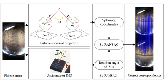
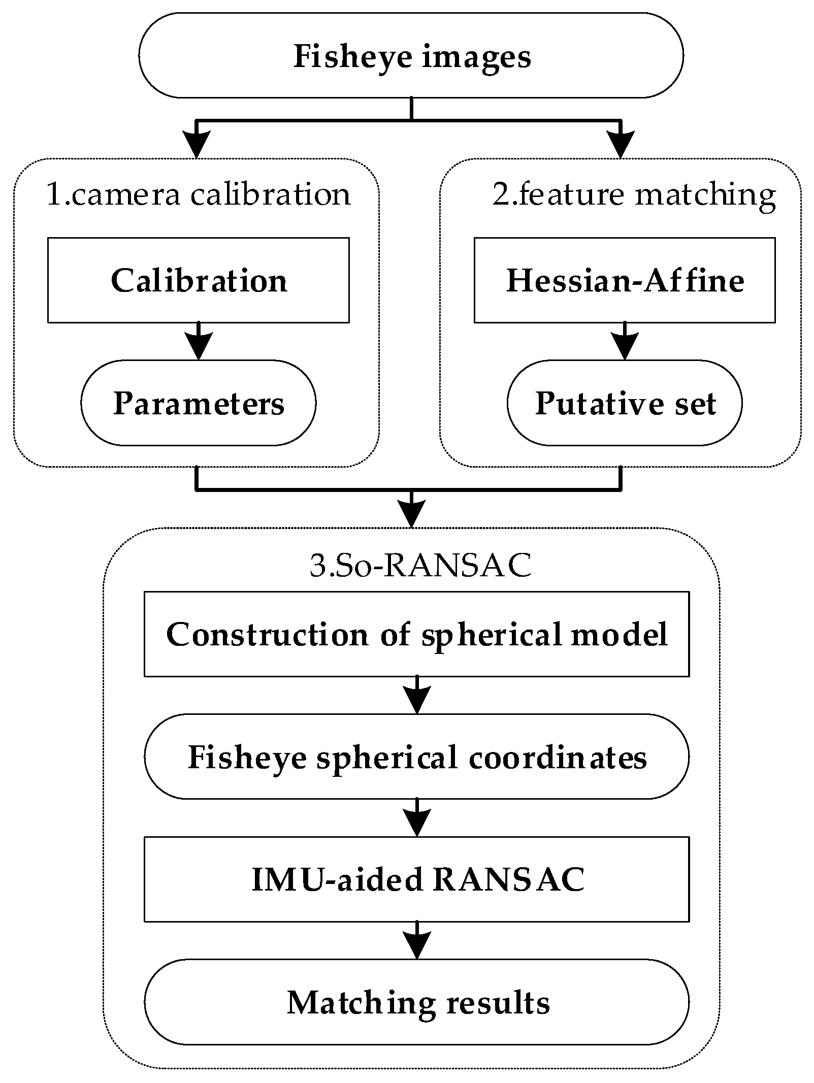
The motivation for this paper was to explore an inertial-assisted matching method suitable for fisheye images in view of the limitations of the previous multi-sensor-assisted matching method. The So-RANSAC algorithm proposed in this paper was inspired by previous works [22,28,29,30]. This method can be divided into three stages: (1) fisheye model construction: the internal parameters and the distortion parameters of the fisheye camera were obtained by calibration, and the fisheye camera imaging model was recovered from the fisheye image; (2) image feature matching: feature points were extracted by an affine-invariant detector; (3) outlier removal: So-RANSAC method was proposed to construct the fisheye spherical coordinates, and then outliers were removed. Compared with the previous methods, So-RANSAC not only improves the outlier removal accuracy by using the IMU, but also has good adaptability to fisheye distortion. The main innovation of this paper is the construction of a fisheye spherical model that restores the fisheye epipolar constraints and improves the outlier removal accuracy. The overall process of our method is shown in Figure 1.
3.1. Camera Model and Feature Matching
Fisheye camera models do not conform to the perspective geometry; that is, they do not conform to the collinear condition, so the fundamental matrix or essential matrix under the perspective geometry cannot be directly applied to fisheye images. To handle this problem, the fisheye camera needs to be calibrated, and the two-view geometry needs to be restored based on a specific model. Therefore, in this stage, the fisheye camera calibration method proposed in [7] was adopted. The principle can be expressed as:
where (u, v) represents the image pixel coordinates, X represents the world coordinates, f(u, v) is a function related to , ρ is the distance from (u, v) to the principal point of the image, a0, a1,∙∙∙, an is the set of coefficients to be calculated (usually, n = 5), and P is the projection matrix. After calibration, a collinear relationship is established between the pixel coordinates of the points in the fisheye image and the world coordinates of the spatial points.
[u, v, f(u, v)] = PX
f(u, v) = a0 + a1ρ + a2ρ2+∙∙∙+ anρn
In the feature matching stage, the Hessian–Affine detector [18] is used to extract feature points. The principle of the Hessian–Affine algorithm is that the deformation between the local regions of fisheye images can be approximated by an affine transformation. Based on this principle, affine regularization is carried out on the local regions of extracted features to reduce the influence of deformation on feature description. Finally, the extraction and matching of feature points are completed, and the putative correspondence set is obtained.
3.2. Fisheye Image Matching Aided by an IMU
In the outlier removal stage, we propose So-RANSAC to remove outliers while correctly estimating poses. Traditional RANSAC first randomly extracts a minimum sample from the putative set to estimate a pose model and then divides inliers and outliers based on this model. The optimal pose is constructed through an iterative process of sample selection and estimation. However, traditional RANSAC is sensitive to a high proportion of outliers, and the pose estimation step is based on perspective geometry. In this paper, RANSAC is improved by projecting the fisheye image correspondences onto a sphere and restoring the epipolar geometry for pose estimation, and the matching process is assisted by an IMU.
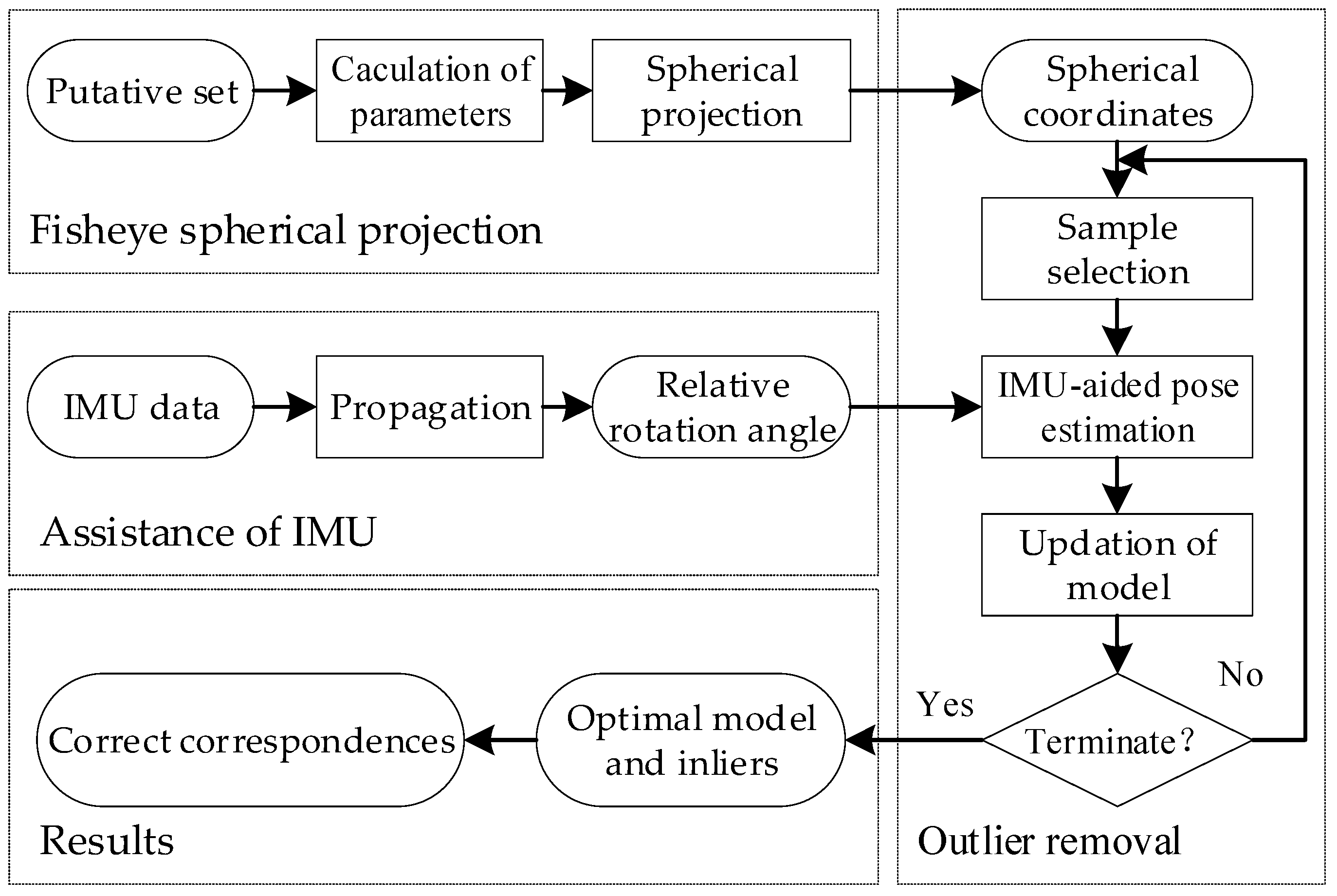
The process of So-RANSAC is shown in Figure 2. The putative correspondence set is converted into spherical coordinates in the fisheye spherical projection part; the relative rotation angle is obtained by IMU propagation in the assistance of the IMU part as a constraint of pose estimation. By combining the above two parts, four-point RANSAC [30] is used to remove outliers, and, finally, the matching result is obtained.
3.2.1. Fisheye Spherical Projection
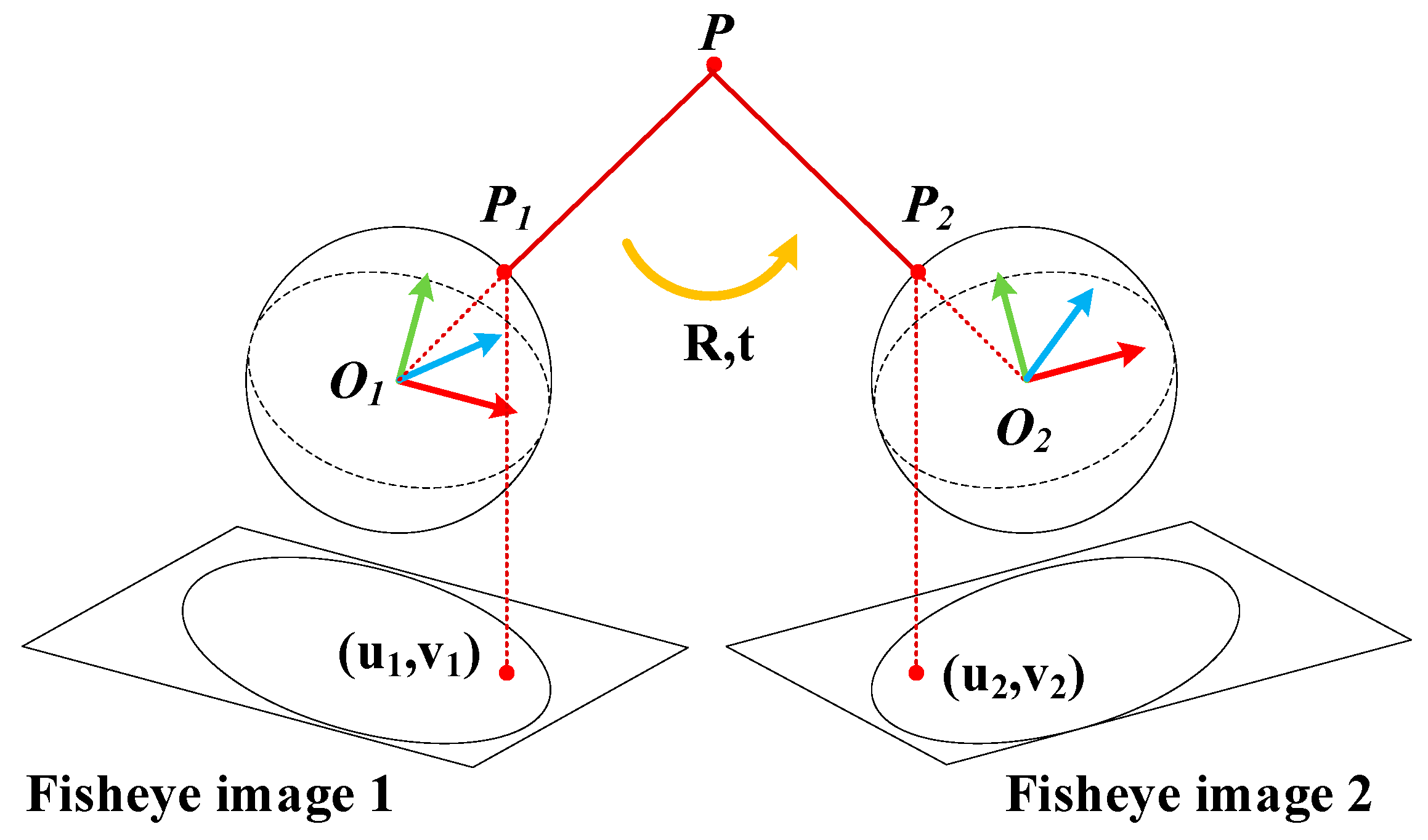
The fisheye images undergo severe distortions such that the perspective geometry of rectilinear perspective images cannot be directly applied to fisheye images [34]. Specific projections (e.g., panoramic or log-polar) can reduce the distortions, while the spherical projection is a non-deformed model for the fisheye images. The projection of the visual information on the sphere correctly handles the information without introducing distortion [21]. Therefore, we adopted the spherical projection to restore the epipolar geometric relationship of the fisheye image and apply the RANSAC method to the fisheye image. The projection of image coordinates onto a sphere was conducted on the basis of calibration as shown in Figure 3.
Fisheye cameras can be modeled by a unit sphere and a perspective camera [9], which means the fisheye imaging process can be performed in two steps: First, we project the world points onto the unit sphere. This step is similar to perspective cameras and conforms to the collinear condition. Then, points on the unit sphere are projected onto the fisheye image plane, and fisheye distortion is mainly produced in this step.
According to this imaging process of a fisheye camera, we can also restore the fisheye epipolar geometry in two steps: First, we reproject the image points back to the unit sphere through calibration to avoid the influence of distortion. Then, we can restore the collinear relationship between the spherical points and the world points.
In Figure 3, (u1, v1) is the image pixel coordinates of world point P. (u1, v1), P1, and P do not satisfy the collinear condition due to the influence of fisheye distortion. Under the calibration model [7], f(u, v) was used to represent the image distortion. We converted an image pixel point (u, v) to the point (u, v, f(u, v)) on the sensor plane thus taking the fisheye distortion into consideration. The point (u, v, f(u, v)) is related to a ray emanating from the viewpoint O to the world point, and this relation is expressed by Formula (1). Therefore, the points on the sensor plane and the world points conform to the perspective projection. Finally, we normalized the points on the sensor plane to the unit sphere. Through the above process, we modeled the fisheye distortion and restored the collinear condition. The details are as follows: According to Formula (1), the coordinates (u, v, f(u, v)) restore the collinear geometry by calibration [7]. (u, v, f(u, v)) are normalized to the unit sphere and converted into spherical coordinates (Xs, Ys, Zs) for the subsequent implementation of the pose estimation algorithm. The normalization and projection are accomplished by the following formula:
where (u1, v1) and (u2, v2) are the image pixel coordinates of world point P projected onto fisheye images A and B. The fisheye camera is calibrated to obtain (u1, v1, f(u1, v1)) and (u2, v2, f(u2, v2)), and the spatial coordinates are normalized to spherical coordinates O1 and O2 to obtain P1(Xs1, Ys1 Zs1) and P2(Xs2, Ys2 Zs2), so the collinear relationship can be reconstructed, and the relative motion between the two fisheye images can be described by essential matrix. By combining this spherical model and the IMU-aided RANSAC, we extend the RANSAC method for rectilinear perspective images and propose the So-RANSAC with fisheye distortion adaptability.
[Xs, Ys, Zs)] = [u, v, f(u, v)]/n
3.2.2. Relative Rotation Angle
The IMU can obtain accurate short-term poses, so when the accuracy of visual pose estimation is not good, the pose obtained by the IMU is used as the constraint of RANSAC to improve the matching accuracy.
In this paper, the theoretical basis of IMU-aided matching was the invariance of the rotation angle of a rigid body in different coordinate systems [35]. It was further proved in [30] that when the camera and IMU are fixed, the rotation angle obtained by the IMU can be directly regarded as the rotation angle of the camera without the need for camera-IMU calibration. Based on this theory, we first used the IMU affixed to the camera to obtain the measurement data, then Madgwick’s method [36] was used to obtain the attitude, and, finally, we converted the attitude into the equivalent rotation vector and rotation angle in which the rotation angle was used to assist with outlier removal.
The complete propagation of the IMU state is complex; thus, for the sake of clarity, we used a simplified navigation equation to describe the IMU orientation propagation:
where is the attitude matrix of IMU, which represents the conversion from the body frame (b) to the navigation frame (n), and is the real angular velocity measured by the IMU, and × represents the conversion of the vector into the skew-symmetric matrix. The change in attitude over time is described by Equation (5).
After the attitude at each moment of the IMU is obtained by IMU propagation, the relative transformation between the attitudes of adjacent moments is calculated to obtain the rotation matrix R. R describes the relative motion between of adjacent moments, and then R is expressed as a function of the equivalent rotation vector ϕ by Rodrigue’s rotation formula [37].
where ϕ represents the three-dimensional equivalent rotation vector, the vector direction of the equivalent rotation vector represents the direction of the axis of rotation, and the magnitude of the norm ‖ϕ‖ represents the magnitude of the rotation angle.
3.2.3. RANSAC Aided by the IMU
RANSAC estimates the essential matrix, E, through a five-point method. For a correspondence s and s’, the two-view geometry is described by the essential matrix:
where t represents the displacement, [t]× represents the skew-symmetric matrix, and R represents the rotation matrix. The essential matrix E has 5 degrees of freedom, and at least 5 correspondences are needed to estimate it.
s Es’ = 0
E = [t]×R
The rotation matrix is expressed by Rodriguez’s rotation formula. The vector direction of the equivalent rotation vector ϕ in Formula (6) is expressed by the unit rotation axis vector μ in three-dimensional space, the magnitude of the norm ‖ϕ‖ is expressed by the rotation angle θ, and the rotation matrix is described by R(θ, μ). At the same time, according to Lie Algebras [38], the skew-symmetric matrix is rewritten by Formula (9), Formula (6) is transformed into Formula (10), and Formula (8) is converted into Formula (11):
([μ]×)2 = μ μT − I
R(θ, μ) = (cos θ)I + (1 − cos θ) μ μT + (sin θ)[μ]×
E(θ, μ, t) = [t]× R(θ, μ)
To estimate E(θ, μ, t), the parameters to be calculated are the rotation angle θ, unit rotation axis vector μ = (μx, μy, μz)T, and displacement t = (tx, ty, tz)T, for a total of 7 unknowns. Since the scale is unknown, μ and t are normalized, so there are 5 degrees of freedom. For the RANSAC task, the reduction in the degree of freedom means the reduction in the number of points required in the minimum sample set, and the influence of the outliers is reduced, so fewer iterations are required, and the theoretical accuracy of the method will also be improved [30]. We adopted four-point RANSAC to estimate E(θ, μ, t), and we provided the rotation angle θ through the IMU to reduce the degrees of freedom of pose estimation. After introducing θ, E had only 4 degrees of freedom, and 4 correspondences were required to estimate the pose, which simplified the calculation. Subsequently, the obtained pose model was used to calculate the reprojection error of each point in the putative set, and the inliers and outliers were classified. After iterating, the optimal pose and inliers set were finally obtained.
The above content is the principle of the So-RANSAC algorithm on the fisheye spherical point set S; the algorithm flow is shown in (Algorithm 1).
| Algorithm 1. So-RANSAC aided by IMU |
| Input: putative set M, relative rotation angle θ, fisheye camera calibration parameters |
| Initialization: |
| 1. The putative set M is projected onto the sphere, and the spherical set S is obtained |
| 2. for i=1:N do |
| 3. Select a minimum sample set (4 correspondences) from S |
| 4. The essential matrix E is estimated, and the attitude of the model is given by θ |
| 5. The reprojection error of S is calculated according to model E, and the number of inner points Ninliers is calculated. |
| 6. The model with the largest Ninliers is regarded as the best model |
| 7. end for |
| 8. Save the optimal model Eoptimal and the inliers |
| Output: Inliers |
In summary, the method proposed in this paper adopted four-point RANSAC to integrate the IMU and visual information, and we used the IMU to improve the effect of outlier removal. This did not require camera–IMU calibration, which was convenient to apply. More importantly, the reliability of the epipolar constraint was improved by constructing the fisheye spherical coordinate model, and the accuracy of RANSAC was improved.
4. Results
4.1. Experimental Data
To verify the method proposed in this paper (So-RANSAC), image matching experiments were carried out in a real application and using public data sets.
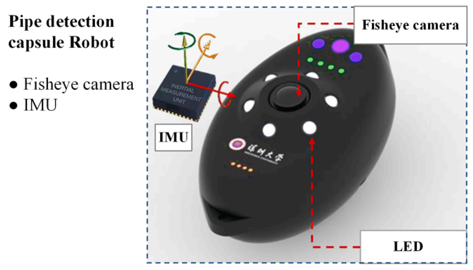
The real application was the detection of urban drainage pipes. The fisheye images of the drainage pipe were acquired by a self-developed pipe capsule robot. The robot had a small, portable structure and traveled in the pipeline by drifting; it also had a high work efficiency and autonomously localized and detected pipeline issues. An IMU and a fisheye camera were integrated into the robot. The type of IMU was an ICM-20689 high-performance six-axis microelectromechanical systems (MEMS), and the fisheye lens was a high-definition 220° wide-angle lens. The main hardware specifications of the capsule robot are shown in Table 1.
The appearance of the capsule robot is shown in Figure 4. The original data taken by the robot were 1080p video data, and the frame rate was 60 frames per second. The video was sampled at 30 frames per second to obtain discrete fisheye images as shown in Figure 5. Due to the complex internal environment of drainage pipes, the factors that affected the fisheye image matching problem included motion blur and lens occlusion caused by the water environment, fisheye distortion, and the lack of texture caused by the pipe surface material. Therefore, the fisheye image matching task of this scene was challenging.
In addition, we used fisheye images from the Technical University of Munich’s (TUM) monocular visual odometry data set [39]. The scene in the data set is an indoor environment. Compared with the pipeline data, the TUM images have richer textures, no violent motion artifacts, and better image quality as shown in Figure 6. This data set was selected for comparison to verify the robustness of the proposed method in different scenarios. The TUM data set provided the ground truth of the camera pose, that is, the absolute pose information at each moment, and the poses are represented by quaternions. In this experiment, the quaternion data were converted into relative rotation angles, which are regarded as auxiliary information.
4.2. Image Matching Results
The ground truth of the fisheye image matching experiment was manually selected to ensure correctness. The So-RANSAC was compared with RANSAC [5] and the current state-of-the-art methods: LPM [25], vector field consensus (VFC) [24], and four-point RANSAC [30]. The matching quality was evaluated through the precision, recall, and F-score, which were calculated by Formulas (12)–(14). In addition, we counted the number of correct matches (NCMs) and the success rate (SR) as the evaluation metrics.
For the parameter settings of each matching method, the confidence of the RANSAC-type methods was set to 0.99, and the threshold of the reprojection error of the inliers during iteration was set to 3 pixels. The parameters of the LPM and VFC algorithms were set according to the default parameters of the source code provided by the authors. The IMU measurements in the pipeline were processed in accordance with the method in Section 3.2.2, using Madgwick’s method [36] to obtain the attitude at each moment and then converted to the relative rotation angle. The TUM data set provided the ground truth of the attitude, which was directly converted into the relative rotation angle. Detailed information on the experiment is shown in Table 2.
The average number of correct matches (NCMs) and the success rate (SR) of matches were calculated on the pipeline data set as shown in Table 3. To calculate the matching success rate, we first estimated the correct pose using the correspondences of the ground truth; then, we calculated the residuals of the putative correspondences under the estimated pose of the ground truth and regarded the correspondences with residuals less than 3 pixels as the correct matches. If the number of correct matches of an image pair was less than four, we considered that the match had failed. Due to the complex characteristics of pipeline images (e.g., motion blur, fisheye distortion, and the lack of texture), the RANSAC-type methods may fail when the number of correct correspondences is less than four pairs or there are too many outliers. Therefore, the matching success rate of the three RANSAC-type methods was only 96%. The introduction of IMU assistance did not improve this situation, but it did increase the number of correct matches. The LPM and VFC methods are based on local geometric constraints, so they are more adaptable to these situations, and their matching success rates were both 100%, and they retained more correct matches than RANSAC-type methods. However, it should be noted that although the matching success rate can reflect the adaptability of the matching method under harsh conditions, if the restriction is too loose, the high matching success rate may also lead to undiscovered outliers. Therefore, in order to measure the performance of the matching methods, it is also necessary to consider other evaluation metrics (e.g., precision and recall).
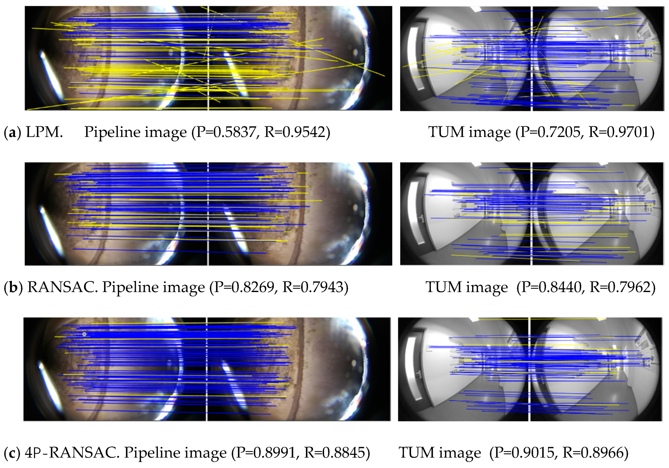
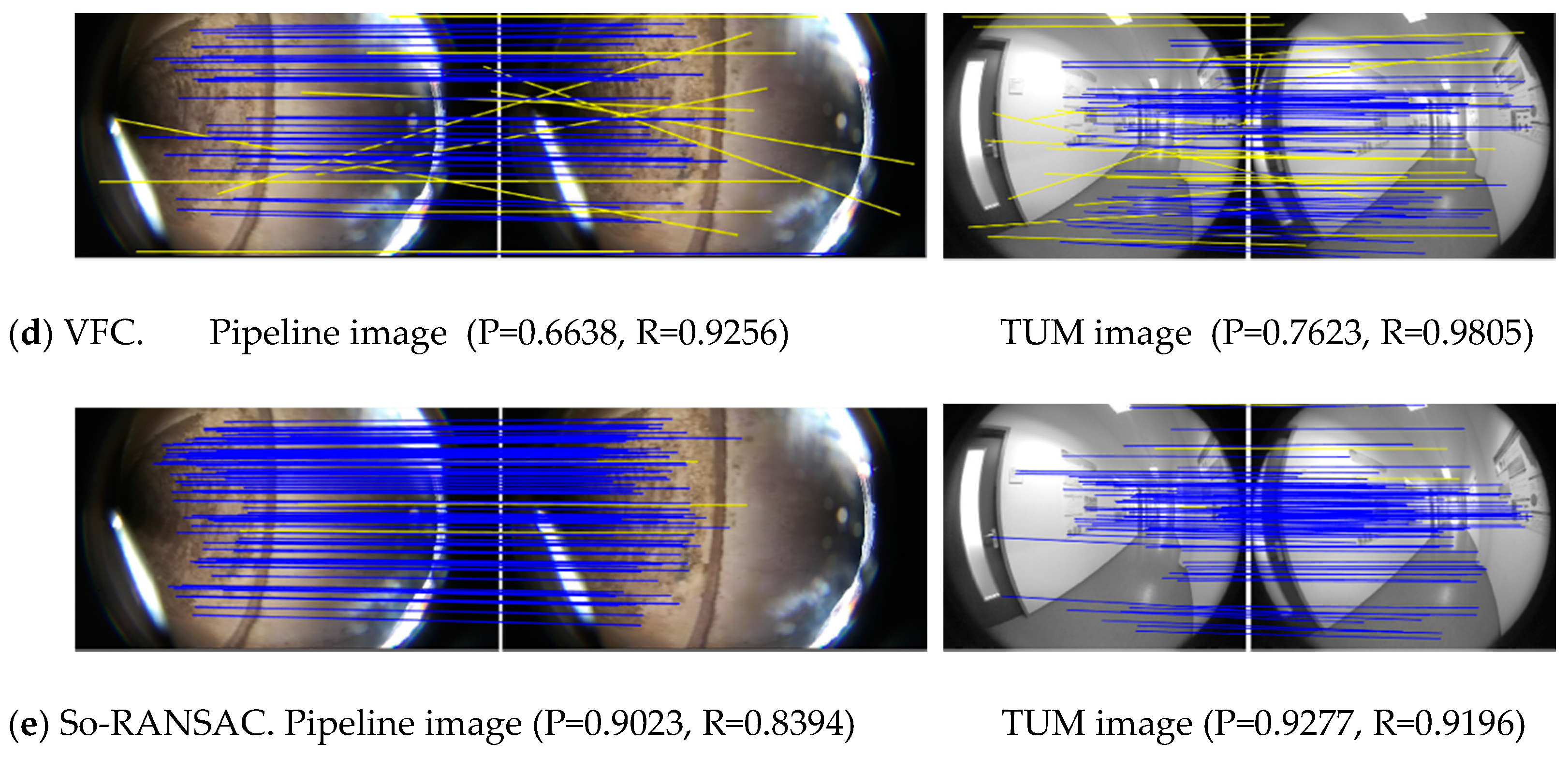
Figure 7 shows the matching results of sample image pairs selected from the pipeline and TUM data sets. In the pipeline image matching example in Figure 7, the LPM algorithm considered only the geometric consistency in the local area (usually within a few pixels), and the precision was only 58.37% in the case of repeated texture in the pipeline image. However, due to the fact of its loose geometric restrictions, the recall reached 95.42%. The VFC algorithm assumed that the correct matching points should conform to the same vector field model, but due to the serious distortion in fisheye images, this assumption was inaccurate, so the precision was only 66.38%. However, it is worth mentioning that although the accuracy of the above two methods is not high, they have a high recall and can retain most of the correct correspondences. Therefore, in tasks requiring real-time performance, they can be used as coarse matching method to provide initial values for subsequent optimization. RANSAC, four-point RANSAC, and So-RANSAC have the same basic principles, but the difference lies in two points: whether to use IMU assistance and whether to use a fisheye spherical model. Neither RANSAC nor four-point RANSAC adopted the fisheye model; the precision of RANSAC was 82.69%, and the precision of four-point RANSAC improved to 89.91% after the addition of IMU assistance. The So-RANSAC method adopted fisheye spherical coordinates in the pose estimation stage, which was more adaptive to distortions, so the precision improved to 90.23%, thus indicating the feasibility of this spherical model.
In the example of the TUM data set image in Figure 7, the performance of each matching method is relatively improved due to the better image quality and richer texture. By comparison, the precision values of the LPM and VFC algorithm were still relatively lower than those of the RANSAC-type methods, but the recall values were high. The So-RANSAC method still outperformed RANSAC and four-point RANSAC.
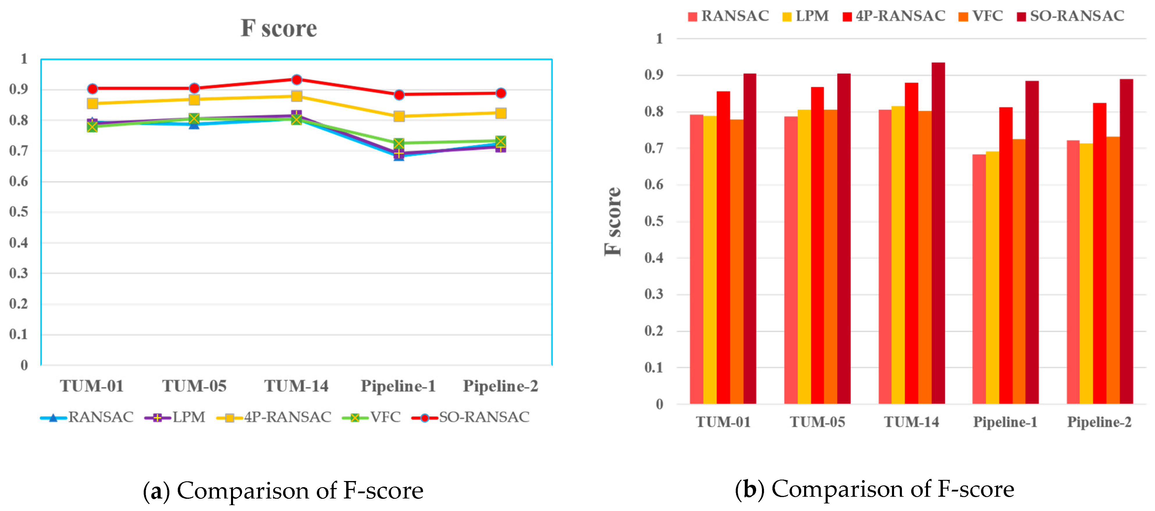
Figure 8 and Figure 9 quantitatively compare the precision, recall, and F-score of each method in five sets of experimental data (the detailed information on the five sets are shown in Table 2). For each set, we calculated the mean value of the matching results of all the images (precision, recall, and F-score), and displayed them via line chart and histogram. Finally, all the data were integrated to calculate the overall precision, recall, and F-score, which are shown in Table 4.
By comparison, it can be seen from Table 5 that the precision of the LPM algorithm was 66.49%, but the recall was 96.82%, which was the highest among the five methods. The VFC algorithm was sensitive to distortion, and its precision was the lowest (65.57%). So-RANSAC achieved the best performance with a precision of 92.57% and a recall of 88.41%; its F-score was 90.44%, both precision and F-score were the highest. The performance of four-point RANSAC ranked second; the precision and the recall of four-point RANSAC were better than those of RANSAC with IMU assistance, and the F-score was 85.53%. The precision of RANSAC was 83.26%, which was better than that of the LPM and VFC algorithms, but the recall was the lowest (75.73%).
In addition, the performance of the five methods on the TUM data set was superior to their performance on the pipeline data, because the image quality was better and the image textures were richer in the TUM data set. In addition, the motion blur and repeated textures of the pipeline images reduced the matching accuracy. In general, the So-RANSAC method had good performance in real and experimental scenes and was robust to complex environments.
4.3. Reprojection Error
RANSAC-type methods carry out pose estimation while removing outliers, and the result can be used as the initial value in visual odometry or simultaneous localization and mapping (SLAM). To verify the pose estimation accuracy, the correspondences of the ground truth in all the image pairs were reprojected according to the estimated pose, and the reprojection error vi was calculated. Reprojection errors of RANSAC, four-point RANSAC and So-RANSAC were compared and evaluated by calculating the 𝑚𝑒𝑎𝑛 𝑎𝑏𝑠𝑜𝑙𝑢𝑡𝑒 𝑒𝑟𝑟𝑜𝑟 (MAE) and 𝑟𝑜𝑜𝑡 𝑚𝑒𝑎𝑛 𝑠𝑞𝑢𝑎𝑟𝑒 𝑒𝑟𝑟𝑜𝑟 (RMSE) of the ground truth points set.
Detailed information on the experiment is shown in Table 5. The experiment shows that the reprojection error of four-point RANSAC was smaller than that of RANSAC, indicating that IMU assistance can improve the pose estimation accuracy, while So-RANSAC achieved the optimal result, indicating that the fisheye spherical model was helpful for enhancing the adaptability to distortion and improving the pose estimation accuracy.
4.4. Computation Time
In terms of the computation time, we recorded the runtimes of the various algorithms on 100 pipeline images and compared the average runtimes. The computational efficiency results are shown in Table 6. The time complexity of the LPM algorithm was O( N log(N) ), which was the fastest, and the average matching time was only 0.013 s, but the accuracy was the lowest. The time complexity of the VFC algorithm was O(N3), which ranked second in terms of efficiency. The iterative solution process of RANSAC resulted in a relatively slow computational efficiency, which was more than 10 times that of the LPM algorithm, but the average efficiency was still controlled within 1 s, and the matching accuracy was higher. The four-point RANSAC algorithm with the addition of IMU assistance increased the average runtime to 0.651 s, while the So-RANSAC algorithm with the addition of the spherical model increased the average time to 0.719 s. It is worth mentioning that the RANSAC-type methods can obtain inliers and pose at the same time, which can provide an accurate initial value for subsequent bundle adjustment of SLAM and make it converge faster. Therefore, RANSAC-type methods are more suitable for tasks requiring localization than other nonparametric methods.
5. Discussion
The IMU will inevitably produce errors in the measurement process. Since this paper focused on the outlier removal method using visual information, and the relative rotation angle provided by the IMU was only used for the relative restriction in the epipolar geometric, we did not analyze the IMU errors in detail. In this chapter, the influence of IMU error on matching accuracy is discussed theoretically and experimentally.
In general, translation estimation of IMU is much more sensitive to noise compared to rotation estimation, and the relative rotation measurements are more stable. In addition, we only used IMU information as auxiliary information to improve the accuracy of outlier removal. In the estimation of E(θ, t), although the error of θ will affect the accuracy in theory, in practice this effect will not be obvious when the error is small. Since the errors of IMU are time dependent, long-term pose estimation will cause trajectory drift and error divergence, but the effect of the error on the pose estimation in the short time is tolerable. The sampling interval between two images in this paper was only 1/30s, and in this short time interval, the influence of the IMU error on RANSAC would not be significant.
We carried out comparative experiments to show how the noise from the IMU influences the accuracy of the So-RANSAC method, and the experimental results are shown in Table 7. Due to the limitations of the pipeline environment and equipment, it was difficult to obtain the ground truth of pipeline data at present. Therefore, we compared the matching precisions of So-RANSAC using the pose obtained by Madgiwick’s method (MARG) and the Kalman-based algorithm (Kalman), and we discuss the impact of IMU error on matching results. We used the open-source codes in [36] to implement the above methods. It was proved in [36] that the MARG method has higher accuracy than Kalman-based algorithm, so the results of Kalman can be regarded as data with greater noise. In addition, we set-up simulation data for comparison. We assumed that the relative rotation angle θ (obtained by MARG) was measured as (1 + e)θ by the IMU, where e reflects the noise, and we set e as 0.02. In practice, the error of θ provided by IMU was much smaller than e. Therefore, through this simulation experiment, the influence of the IMU noise on So-RANSAC can be better tested.
As shown in Table 7, the precision of MARG was improved by approximately 0.1% than that of Kalman, and the average correct matching number was improved by 0.14 pairs, while the matching success rate remains unchanged, indicating that small IMU errors have indeed affected the matching precision, but the impact was small. By comparing the simulation data (1 + e)θ with the MARG method, it can be seen that when the error increased, the average number of correct matches decreased by approximately 1 pair, and the matching precision decreased by approximately 7%, but the matching success rate still remains unchanged. This is because the failure of RANSAC usually occurred when the number of correct correspondences was less than four or there were too many outliers (the rate of the outlier was higher than 90%). Therefore, the above experiments indicate that small IMU errors in a short period of time will not cause serious impacts on the matching result.
How to integrate IMU errors into the matching model is a meaningful research direction. In visual-inertial SLAM, the IMU error is eliminated through a tightly coupled optimization process. In photogrammetry, the IMU error can be eliminated by bundle adjustment. However, since the focus of this paper is on the matching of two images, overall optimization is not the focus of this paper. Meanwhile, due to the limitations of current equipment, data and theory, at this stage we have not integrated the IMU error into the matching model, which is a limitation of our method. However, this limitation does not affect the innovation of our method, the above experiments and discussions are sufficient to indicate the superiority of So-RANSAC in fisheye image matching.
6. Conclusions
To improve the accuracy of fisheye image matching, we proposed an outlier removal method called So-RANSAC, which integrates IMU visual information to deal with the challenge of fisheye distortion. We used the relative rotation angle of the IMU to assist in pose estimation via RANSAC. Then, we introduced fisheye spherical coordinates to reconstruct the fisheye epipolar geometry; this model can enhance the adaptability to distortion and improve the matching quality. We conducted experiments on drainage pipe fisheye images, and the experimental results show that So-RANSAC can accurately remove outliers and achieve robust fisheye image matching results for infrastructure monitoring.
The limitation of So-RANSAC is that the geometric model of IMU-assisted matching can be further improved. At present, only the relative rotation angle was used to reduce the degrees of freedom in pose estimation by one, and the pose information provided by the IMU was not fully utilized. Therefore, there is still much room for improvement in the IMU-aided method to improve the accuracy of fisheye image matching.
Author Contributions
Conceptualization, A.L. and Z.C.; methodology, A.L.; software, A.L.; validation, A.L.; writing—original draft preparation, A.L.; writing—review and editing, Z.C. and Q.L.; visualization, X.F.; supervision, J.Y. and D.Z.; project administration, Q.L. and J.Z. All authors have read and agreed to the published version of the manuscript.
Funding
This research was funded by the China Natural Science Foundation (grant number N2019G012, 41901412) and the National key research and development plan (2019YFB2102703, 2020YFC1512001).
Institutional Review Board Statement
Not applicable.
Informed Consent Statement
Not applicable.
Conflicts of Interest
The authors declare no conflict of interest.
References
- Zhang, Z.; Rebecq, H.; Forster, C.; Scaramuzza, D. Benefit of Large Field-of-View Cameras for Visual Odometry. In Proceedings of the 2016 IEEE International Conference on Robotics and Automation (ICRA), Stockholm, Sweden, 16–21 May 2016; pp. 801–808. [Google Scholar] [CrossRef] [Green Version]
- Hughes, C.; Glavin, M.; Jones, E.; Denny, P. Wide-Angle Camera Technology for Automotive Applications: A Review. IET Intell. Transp. Syst. 2009, 3, 19. [Google Scholar] [CrossRef] [Green Version]
- Liu, Z. State of the Art Review of Inspection Technologies for Condition Assessment of Water Pipes. Measurement 2013, 46, 1–15. [Google Scholar] [CrossRef] [Green Version]
- Zhang, Y.; Hartley, R.; Mashford, J.; Wang, L. Pipeline Reconstruction from Fisheye Images. J. WSCG 9 2011, 19, 49–57. [Google Scholar]
- Nister, D. An Efficient Solution to the Five-Point Relative Pose Problem. IEEE Trans. Pattern Anal. Mach. Intell. 2004, 26, 756–770. [Google Scholar] [CrossRef] [PubMed]
- Ma, J.; Jiang, X.; Fan, A.; Jiang, J.; Yan, J. Image Matching from Handcrafted to Deep Features: A Survey. Int. J. Comput. Vis. 2021, 129, 23–79. [Google Scholar] [CrossRef]
- Scaramuzza, D.; Martinelli, A.; Siegwart, R. A Flexible Technique for Accurate Omnidirectional Camera Calibration and Structure from Motion. In Proceedings of the Fourth IEEE International Conference on Computer Vision Systems (ICVS’06), New York, NY, USA, 4–7 January 2006; p. 45. [Google Scholar] [CrossRef] [Green Version]
- Kannala, J.; Brandt, S.S. A Generic Camera Model and Calibration Method for Conventional, Wide-Angle, and Fish-Eye Lenses. IEEE Trans. Pattern Anal. Mach. Intell. 2006, 28, 1335–1340. [Google Scholar] [CrossRef] [Green Version]
- Puig, L.; Bermúdez, J.; Sturm, P.; Guerrero, J.J. Calibration of Omnidirectional Cameras in Practice: A Comparison of Methods. Comput. Vis. Image Underst. 2012, 116, 120–137. [Google Scholar] [CrossRef] [Green Version]
- Zhang, X.; Zhao, P.; Hu, Q.; Ai, M.; Hu, D.; Li, J. A UAV-Based Panoramic Oblique Photogrammetry (POP) Approach Using Spherical Projection. ISPRS J. Photogramm. Remote Sens. 2020, 159, 198–219. [Google Scholar] [CrossRef]
- Zhao, Q.; Wan, L.; Feng, W.; Zhang, J.; Wong, T.-T. Cube2Video: Navigate Between Cubic Panoramas in Real-Time. IEEE Trans. Multimed. 2013, 15, 1745–1754. [Google Scholar] [CrossRef]
- Ha, S.J.; Koo, H.I.; Lee, S.H.; Cho, N.I.; Kim, S.K. Panorama Mosaic Optimization for Mobile Camera Systems. IEEE Trans. Consum. Electron. 2007, 53, 9. [Google Scholar] [CrossRef] [Green Version]
- Coorg, S.; Teller, S. Spherical Mosaics with Quaternions and Dense Correlation. Int. J. Comput. Vis. 2000, 37, 259–273. [Google Scholar] [CrossRef]
- Lowe, D.G. Distinctive Image Features from Scale-Invariant Keypoints. Int. J. Comput. Vis. 2004, 60, 91–110. [Google Scholar] [CrossRef]
- Rublee, E.; Rabaud, V.; Konolige, K.; Bradski, G. ORB: An Efficient Alternative to SIFT or SURF. In Proceedings of the 2011 International Conference on Computer Vision, Barcelona, Spain, 6–13 November 2011; IEEE: Barcelona, Spain, 2011; pp. 2564–2571. [Google Scholar] [CrossRef]
- Furnari, A.; Farinella, G.M.; Bruna, A.R.; Battiato, S. Distortion Adaptive Sobel Filters for the Gradient Estimation of Wide Angle Images. J. Vis. Commun. Image Represent. 2017, 46, 165–175. [Google Scholar] [CrossRef]
- Puig, L.; Guerrero, J.J.; Daniilidis, K. Scale Space for Camera Invariant Features. IEEE Trans. Pattern Anal. Mach. Intell. 2014, 36, 1832–1846. [Google Scholar] [CrossRef] [PubMed] [Green Version]
- Mikolajczyk, K.; Tuytelaars, T.; Schmid, C.; Zisserman, A.; Matas, J.; Schaffalitzky, F.; Kadir, T.; Gool, L.V. A Comparison of Affine Region Detectors. Int. J. Comput. Vis. 2005, 65, 43–72. [Google Scholar] [CrossRef] [Green Version]
- Furnari, A.; Farinella, G.M.; Bruna, A.R.; Battiato, S. Affine Covariant Features for Fisheye Distortion Local Modeling. IEEE Trans. Image Process. 2017, 26, 696–710. [Google Scholar] [CrossRef]
- Arican, Z.; Frossard, P. Scale-Invariant Features and Polar Descriptors in Omnidirectional Imaging. IEEE Trans. Image Process. 2012, 21, 2412–2423. [Google Scholar] [CrossRef] [Green Version]
- Cruz-Mota, J.; Bogdanova, I.; Paquier, B.; Bierlaire, M.; Thiran, J.-P. Scale Invariant Feature Transform on the Sphere: Theory and Applications. Int. J. Comput. Vis. 2012, 98, 217–241. [Google Scholar] [CrossRef]
- Lourenco, M.; Barreto, J.P.; Vasconcelos, F. SRD-SIFT: Keypoint Detection and Matching in Images with Radial Distortion. IEEE Trans. Robot. 2012, 28, 752–760. [Google Scholar] [CrossRef]
- Fitzgibbon, A.W. Simultaneous Linear Estimation of Multiple View Geometry and Lens Distortion. In Proceedings of the 2001 IEEE Computer Society Conference on Computer Vision and Pattern Recognition, CVPR 2001, Kauai, HI, USA, 8–14 December 2001; pp. I-125–I-132. [Google Scholar] [CrossRef]
- Ma, J.; Zhao, J.; Tian, J.; Yuille, A.L.; Tu, Z. Robust Point Matching via Vector Field Consensus. IEEE Trans. Image Process. 2014, 23, 1706–1721. [Google Scholar] [CrossRef] [Green Version]
- Ma, J.; Zhao, J.; Jiang, J.; Zhou, H.; Guo, X. Locality Preserving Matching. Int. J. Comput. Vis. 2019, 127, 512–531. [Google Scholar] [CrossRef]
- Li, J.; Hu, Q.; Ai, M. LAM: Locality Affine-Invariant Feature Matching. ISPRS J. Photogramm. Remote Sens. 2019, 154, 28–40. [Google Scholar] [CrossRef]
- Li, J.; Hu, Q.; Ai, M. 4FP-Structure: A Robust Local Region Feature Descriptor. Photogramm. Eng. Remote Sens. 2017, 83, 813–826. [Google Scholar] [CrossRef]
- Campos, M.B.; Tommaselli, A.M.G.; Castanheiro, L.F.; Oliveira, R.A.; Honkavaara, E. A Fisheye Image Matching Method Boosted by Recursive Search Space for Close Range Photogrammetry. Remote Sens. 2019, 11, 1404. [Google Scholar] [CrossRef] [Green Version]
- Scaramuzza, D.; Fraundorfer, F.; Siegwart, R. Real-Time Monocular Visual Odometry for on-Road Vehicles with 1-Point RANSAC. In Proceedings of the 2009 IEEE International Conference on Robotics and Automation, Kobe, Japan, 12–17 May 2009; pp. 4293–4299. [Google Scholar] [CrossRef]
- Li, B.; Heng, L.; Lee, G.H.; Pollefeys, M. A 4-Point Algorithm for Relative Pose Estimation of a Calibrated Camera with a Known Relative Rotation Angle. In Proceedings of the 2013 IEEE/RSJ International Conference on Intelligent Robots and Systems, Tokyo, Japan, 3–7 November 2013; pp. 1595–1601. [Google Scholar] [CrossRef]
- Valiente, D.; Gil, A.; Reinoso, Ó.; Juliá, M.; Holloway, M. Improved Omnidirectional Odometry for a View-Based Mapping Approach. Sensors 2017, 17, 325. [Google Scholar] [CrossRef] [Green Version]
- Yi, K.M.; Trulls, E.; Ono, Y.; Lepetit, V.; Salzmann, M.; Fua, P. Learning to find good correspondences. arXiv 2018, arXiv:1711.05971. [Google Scholar]
- Pourian, N.; Nestares, O. An End to End Framework to High Performance Geometry-Aware Multi-Scale Keypoint Detection and Matching in Fisheye Imag. In Proceedings of the 2019 IEEE International Conference on Image Processing (ICIP), Taipei, Taiwan, 22–25 September 2019; pp. 1302–1306. [Google Scholar] [CrossRef]
- Liu, S.; Guo, P.; Feng, L.; Yang, A. Accurate and Robust Monocular SLAM with Omnidirectional Cameras. Sensors 2019, 19, 4494. [Google Scholar] [CrossRef] [PubMed] [Green Version]
- Chen, H.H. A Screw Motion Approach to Uniqueness Analysis of Head-Eye Geometry. In Proceedings of the 1991 IEEE Computer Society Conference on Computer Vision and Pattern Recognition, Maui, HI, USA, 3–6 June 1991; pp. 145–151. [Google Scholar] [CrossRef]
- Madgwick, S.O.H.; Harrison, A.J.L.; Vaidyanathan, R. Estimation of IMU and MARG Orientation Using a Gradient Descent Algorithm. In Proceedings of the 2011 IEEE International Conference on Rehabilitation Robotics, Zurich, Switzerland, 29 June–1 July 2011; pp. 1–7. [Google Scholar] [CrossRef]
- Hartley, R.; Zisserman, A. Multiple View Geometry in Computer Vision; Cambridge University Press: Cambridge, UK, 2003. [Google Scholar]
- Iachello, F. Lie Algebras and Applications; Lecture Notes in Physics; Springer: Berlin/Heidelberg, Germany, 2015; Volume 891. [Google Scholar] [CrossRef] [Green Version]
- Matsuki, H.; von Stumberg, L.; Usenko, V.; Stuckler, J.; Cremers, D. Omnidirectional DSO: Direct Sparse Odometry With Fisheye Cameras. IEEE Robot. Autom. Lett. 2018, 3, 3693–3700. [Google Scholar] [CrossRef] [Green Version]
Figure 1.
Overall flowchart of the fisheye image matching method.

Figure 2.
Flowchart of the So-RANSAC.

Figure 3.
The fisheye spherical projection.

Figure 4.
The appearance of the capsule robot.

Figure 5.
The fisheye images obtained by the capsule robot.

Figure 6.
The fisheye images from the TUM data set.

Figure 7.
Examples of the matching results. (a–e) show the results of the matching methods. The left column shows the results on a pipeline image pair, and the right column shows the results on a TUM image pair. The blue lines indicate correct correspondences, and the yellow lines indicate outliers. For good visualization, only parts of the correspondences are displayed. (P represents the precision, and R represents the recall).


Figure 8.
Precision and recall of each method in the five sets of experimental data: (a) precision and (b) recall.
Figure 8.
Precision and recall of each method in the five sets of experimental data: (a) precision and (b) recall.

Figure 9.
F-score of each method in the five sets of experimental data: (a) line chart and (b) histogram.
Figure 9.
F-score of each method in the five sets of experimental data: (a) line chart and (b) histogram.


Table 1.
Main parameters of the capsule robot.
| Main Components of the Robot | Parameters |
|---|---|
| CMOS | IMX274 1080p HD sensor |
| Lens | 220° wide-angle HD lens |
| Video resolution | HD 1080p |
| Frame rate | 1080p 60 fps |
| IMU | ICM-20689 high-performance 6-axis MEMS |
Table 2.
The details of the experimental settings.
| Scheme 1 | Information |
|---|---|
| Parameters | (1) So-RANSAC, Four-point RANSAC, RANSAC: p = 0.99, T = 3 (2) LPM, VFC: default |
| Data sets | (1) TUM data set: sequence_01, 50 images; sequence_05, 50 images; sequence_14, 50 images (2) Pipeline data set 1: 50 images; Pipeline data set 2: 50 images |
| Methods | (1) RANSAC, C++, OpenCV 2.4.9 (2) Four-point RANSAC, C++: https://github.com/prclibo/relative-pose-estimation/tree/master/four-point-groebner (3) LPM, MATLAB: https://github.com/jiayi-ma/LPM (4) VFC, MATLAB: https://github.com/jiayi-ma/VFC |
| Evaluation metrics | Precision; recall; F-score; MAE; RMSE |
Table 3.
The comparison of NCMs and SR on the pipeline data set.
| Method | Correct Matches Number | Success Rate/% |
|---|---|---|
| RANSAC | 127.15 | 96 |
| LPM | 190.45 | 100 |
| Four-Point RANSAC | 147.21 | 96 |
| VFC | 187.19 | 100 |
| So-RANSAC | 165.27 | 96 |
Table 4.
Performance comparison.
| Method | Precision | Recall | F-Score |
|---|---|---|---|
| RANSAC | 0.832693 | 0.757375 | 0.793250 |
| LPM | 0.664963 | 0.968233 | 0.788440 |
| Four-Points RANSAC | 0.888411 | 0.824689 | 0.855364 |
| VFC | 0.655793 | 0.957326 | 0.778377 |
| So-RANSAC | 0.925717 | 0.884100 | 0.904430 |
Table 5.
Comparison of the reprojection error.
| Method | MAE/Pixels | RMSE/Pixels |
|---|---|---|
| RANSAC | 2.757730 | 3.119673 |
| Four-Points RANSAC | 2.208425 | 3.093145 |
| So-RANSAC | 1.595407 | 2.109953 |
Table 6.
Comparison of the reprojection error.
| Method | Times/s |
|---|---|
| LPM | 0.013 |
| VFC | 0.226 |
| RANSAC | 0.373 |
| Four-Points RANSAC | 0.651 |
| So-RANSAC | 0.719 |
Table 7.
Performance comparison under IMU error.
| Method | Correct Matches Number | Success Rate/% | Precision |
|---|---|---|---|
| MARG | 165.27 | 96 | 0.925717 |
| Kalman | 165.13 | 96 | 0.924592 |
| Simulation | 152.55 | 96 | 0.854469 |
Publisher’s Note: MDPI stays neutral with regard to jurisdictional claims in published maps and institutional affiliations. |
© 2021 by the authors. Licensee MDPI, Basel, Switzerland. This article is an open access article distributed under the terms and conditions of the Creative Commons Attribution (CC BY) license (https://creativecommons.org/licenses/by/4.0/).
Share and Cite
MDPI and ACS Style
Liang, A.; Li, Q.; Chen, Z.; Zhang, D.; Zhu, J.; Yu, J.; Fang, X. Spherically Optimized RANSAC Aided by an IMU for Fisheye Image Matching. Remote Sens. 2021, 13, 2017. https://0-doi-org.brum.beds.ac.uk/10.3390/rs13102017
AMA Style
Liang A, Li Q, Chen Z, Zhang D, Zhu J, Yu J, Fang X. Spherically Optimized RANSAC Aided by an IMU for Fisheye Image Matching. Remote Sensing. 2021; 13(10):2017. https://0-doi-org.brum.beds.ac.uk/10.3390/rs13102017
Chicago/Turabian StyleLiang, Anbang, Qingquan Li, Zhipeng Chen, Dejin Zhang, Jiasong Zhu, Jianwei Yu, and Xu Fang. 2021. "Spherically Optimized RANSAC Aided by an IMU for Fisheye Image Matching" Remote Sensing 13, no. 10: 2017. https://0-doi-org.brum.beds.ac.uk/10.3390/rs13102017
Note that from the first issue of 2016, this journal uses article numbers instead of page numbers. See further details here.