1. Introduction
Through-the-wall imaging (TWI) is an application area that exploits penetration of microwave fields through building materials for the detection of humans or other targets hidden behind a wall, in a non-destructive way [
1]. It addresses the needs of safety and surveillance in both civil and military operations. Due to the presence of a wall that separates the radar antennas and the target, the complexity of this imaging problem is enhanced compared to classical microwave imaging of free-space targets, or of targets buried in the subsoil, as in ground penetrating radar (GPR) applications [
2]. Indeed, the scattering response may be strongly affected by the additional dielectric layer [
3,
4], since the electromagnetic signal undergoes significant effects of attenuation and distortion due to the multipath propagation occurring at the wall boundaries. The choice of the operational frequencies also plays an important role, and it is the result of a compromise: a better resolution can be achieved at higher frequencies, but at the expense of increased losses in the wall materials and lower penetration inside the building. These considerations suggest the range 0.3–4 GHz as optimal in many TWI scenarios [
5,
6]. Different hardware architectures can be employed: a pulsed radar, where the source is radiating a wideband signal, or a frequency-stepped approach, where the source field is radiated in a limited number of frequencies.
The aims of TWI reconstruction may be different, according to the implemented approach. In most cases, the goal is the identification of the presence of the targets and the retrieval of their positions and shapes. This can be achieved, for example, through synthetic aperture radar approaches, that exploit beamforming techniques for the localization and imaging of static or moving targets [
7,
8,
9,
10,
11]. Refocusing approaches to compensate image distortions due to multipath [
12,
13,
14] and clutter by wall reflections [
15,
16,
17] have been also considered. The concept of all-directions through-the-wall imaging with a large 2D synthetic aperture has been proposed in [
18], and experimentally validated in [
19]. Recently, the issue of mapping the internal walls of the building’s interior has been considered to improve discrimination between walls and objects [
20].
A different approach to TWI is given by inverse scattering algorithms. The developed algorithms mainly extend inverse scattering approaches of free space by including, in exact or approximate forms, the scattering effects introduced by the wall. In most cases, the scattering problem is tackled under a linearized form, e.g., using the Born or Kirchhoff approximations. This approach leads to a qualitative imaging, i.e., it returns target localization and a reconstruction of geometrical information, as target shape and detection of boundaries. Among the proposed techniques, widely used approaches are based on the truncated singular value decomposition (TSVD) [
21,
22,
23], and linear sampling methods [
24,
25,
26]. Moreover, in [
27,
28,
29] the inverse scattering problems applied to TWI have been cast in the form of stochastic optimization approaches. Linearized TWI approaches can be also applied to the tracking of multiple moving targets, as in [
30]. Strategies to suppress multipath ghosts, useful to improve targets detectability in a high-clutter environment, have been proposed in [
31,
32,
33]. Compressive sensing (CS) has been explored, too, to enhance the reconstruction capabilities of targets in the presence of sparse scenarios [
34,
35,
36]. In these implementations, small, mainly point-like, targets are assumed. Advanced CS formulations have also been proposed to solve the imaging problem in presence of ‘non sparse’ extended targets, as in [
37,
38]. CS applied to a multipath propagation scheme is proposed in [
39], developed in a Bayesian framework. Although in some cases free-space Green’s functions or other simplified formulations may be used in the reconstruction procedures, the adoption of a Green’s function developed for a layered background provides a more accurate reconstruction by fully including the effects of the wall in the reconstruction algorithms [
40,
41,
42]. A further approach is the quantitative imaging, i.e., the reconstruction of the distribution of the dielectric properties of the inspected scenario, which is obtained through fully non-linear inverse scattering techniques [
43,
44,
45,
46]. However, their practical implementation is quite challenging, also due to the wide investigation domains, and the limited-view data available from scanning. Finally, it is worth remarking that in many works, TWI algorithms are mainly validated against synthetic data, provided by numerical approaches. However, only validation against experimental data can assess reliability and limits of the reconstructions, while tackling the several non-idealities of real through-wall environments.
In this paper, a new TWI approach based on an inverse-scattering scheme developed in variable-exponent Lebesgue spaces is presented. In particular, the reconstruction is obtained by means of a hybrid procedure, where the TSVD is combined for the first time with a variable-exponent Landweber-like iterative method (VpLW). More in details, a preliminary image of the scenario is obtained by using the TSVD method, and it is used to build the exponent function of the variable-exponent Lebesgue spaces used in the subsequent Landweber-like scheme. In both steps, a linearized scattering model is adopted, which relies upon the use of the Green’s function for a layered background for an accurate characterization of the multipath effects occurring at the wall boundaries.
In particular, the variable-exponent approach has been chosen since it has been found to provide significant enhancements in the reconstruction capabilities in different microwave imaging configurations [
47,
48]. Indeed, the exploitation of the geometrical properties of the variable-exponent Lebesgue spaces allows introducing non-standard regularization behaviors. For instance, it has been found that small values of the exponent function lead to a sparser reconstruction, which is beneficial for the background part of the imaging domain, whereas higher values (e.g., close to 2) improve the characterization of smooth profiles, such as those often shown by the targets. Moreover, the developed variable-exponent technique adaptively defines the values of the exponent function on the basis of a preliminary image, which in this work is obtained through a direct inversion of the adopted scattering operator by means of a TSVD-based approach.
It is worth remarking that this approach extends the one originally presented in [
41], where however the exponent function was built using a delay-and-sum (DAS) beamforming technique. In that case, however, an approximate propagation model was adopted for characterizing the contribution of the wall, in which straight ray-propagation was assumed and the delays used in the beamforming process were obtained by solving, for every focusing point inside the investigation domain, an optimization problem for computing the shortest electric path from the transmitting–receiving antennas. The new approach has the advantage of allowing to use the same scattering model in both steps, which fully take into account the wall effects without approximations, while keeping the same good reconstruction capabilities of the original method. This also allows reusing the same underlying Green’s matrices, which can be thus precomputed for a given scenario, helping to increase the computational efficiency of the method.
Validation of the proposed TWI algorithm against experimental data is given. An experimental campaign is performed in a laboratory environment simulating a through-the-wall scenario, with a single wall hiding metallic or dielectric targets. A pulsed GPR is used in a fully bistatic mode for scanning the transmitting (TX) and receiving (RX) antenna locations under multi-view and multi-illumination mode. A set of measurements of the field scattered by the wall alone is preliminarily acquired in order to isolate the scattering response by the targets. Furthermore, the measured time-domain data have been pre-processed by using a Fourier transform to obtain the frequency-domain scattered-field data at the receiving antennas locations for a given set of frequencies, which are provided in input to the inversion procedure.
The paper is organized as follows. In
Section 2, the proposed inverse scattering approach is reported. Application of the inversion procedure on experimental data is presented in
Section 3. Conclusions follow in
Section 4.
2. TWI Approach
In the considered imaging problem, one or more targets are located in an investigation area
behind a wall of thickness
and complex dielectric permittivity
.
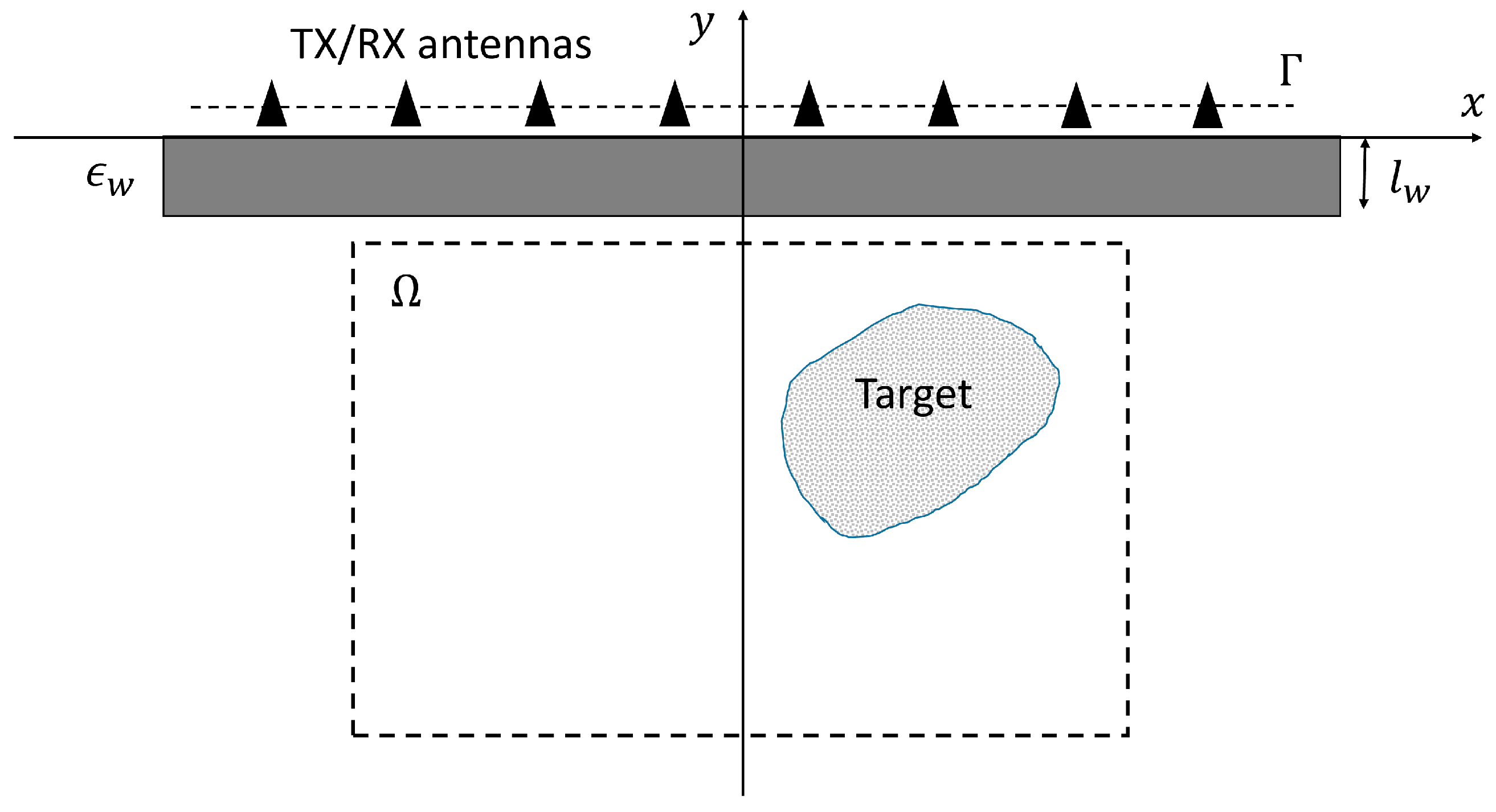
Figure 1 shows a schematic diagram of the adopted configuration. In particular, in this figure, a horizontal cross-section of the scenario is shown, in which the wall is represented by the dark gray box. A two-dimensional configuration is assumed, where the dielectric properties of the targets and of the wall are constant along the z axis. The targets are illuminated by the electric field produced by a set of
antennas positioned in contact with the wall at positions
,
(indicated by the black triangles). In particular, a multi-view multi-illumination setup is considered, in which each antenna is used in turn in TX mode to generate the incident field, whereas the remaining
ones collect the total field produced by the interaction with the wall and the targets. Moreover, it is assumed that data at several working angular frequencies
,
, are available (an
time-dependance is assumed and omitted from now on).
In the following, the TX antennas are modeled as ideal line-current sources, i.e., they generate a transverse-magnetic (TM) electric field with z-component
, where
is the position vector in the transverse plane,
is the magnetic permeability of vacuum,
is the current amplitude, and
is the Green’s function for the assumed three-layer configuration [
49].
Under the previous assumptions, the z-component of the total field collected by the
-th antenna,
, can be expressed in terms of the dielectric properties of the investigation region through a non-linear scalar equation [
2]. However, as often assumed in TWI settings, such a non-linear model can be simplified by using a first-order approximation, leading to the linear equation [
22,
50]
where
is the z-component of the scattered electric field and
is a function depending on the dielectric properties inside the investigation domain
. In particular, when weak scatterers are considered,
is proportional to the contrast function, whereas if strong scatterers are present it assumes high values in correspondence to the targets, thus allowing to obtain an indication of their positions and shapes [
22,
50]. It is worth remarking that (1) relies upon the use of the Green’s function
for a three-layer medium (i.e., a dielectric slab is used to model the wall) [
49], which allows including the wall effects directly in the scattering model. Moreover,
is obtained by subtracting from the total field (i.e., with the wall and the target) the contribution of the wall alone (i.e., the incident field
). Consequently,
contains only information about the targets behind the wall.
By discretizing the investigation domain into square subdomains
,
, of side
in which
is assumed constant, i.e.,
, being
the barycenter of the subdomain
, (1) can be written in discrete form as
where
and
is an array of
elements whose
-th one is given by
Finally, by stacking the equations related to the
illuminations, the
probing antennas, and the
working frequencies, the following discrete problem is attained
where
is an array of length
containing all the available measurements and
is a matrix of dimensions
containing the values of the Green’s function integrals in (3).
In order to obtain an image of the inspected scenario, (4) needs to be inverted for retrieving
. However, such an equation turns out to be severely ill-posed. Consequently, it is necessary to adopt proper regularization schemes. In this work, a hybrid approach is considered. In particular, it is based on a main loop performing a regularization in the framework of the Lebesgue spaces with variable exponent
by means of truncated Landweber-like iterations [
48]. To this end, it is assumed that the unknown space
and is equipped with a Luxemburg norm
defined as [
51]
where
is an array containing the discretized exponent function. Moreover, a constant p-norm
is associated to the data space
, where the parameter
is set equal to the average of
, i.e.,
In order to fully exploit the regularization capabilities of the variable-exponent regularization technique, it is necessary to define a proper exponent function. In particular, as discussed in the Introduction, low values are assigned to the regions belonging to the background, whereas higher ones to the points where a target is located. To this end, an initial image of the scenario, which allows an approximate localization of the targets, is built using a truncated singular value decomposition. The obtained image is then used to define the values of .
The developed VpLW-TSVD hybrid inversion method is summarized by the flow chart in
Figure 2. In particular, the single steps are detailed as follows:
- 1.
Initialization. The solution is initialized with a null vector, i.e., and the iteration index is set to ;
- 2.
TSVD initial reconstruction. An initial preliminary reconstruction is obtained by means of a truncated singular value decomposition as
in which
are the singular values of the matrix
,
and
are the corresponding (left and right) singular vectors, and
is a suitable truncation index;
- 3.
Exponent map construction. Using the initial TSVD reconstruction, the unknown-space exponent function (in discrete form) is computed as
where
and
are the prefixed minimum value and the range of the elements of
, respectively. Moreover, the data-space exponent
is set equal to the average of
according to (6);
- 4.
Iterative update. The solution is iteratively updated as [
47,
48,
52]:
where
is the dual space of
, with
the Hölder conjugate of
,
is the Hermitian transpose of
, and
is a relaxation coefficient that is empirically computed as
In (9),
and
are the duality maps of the spaces
and
, respectively, which are defined as
where
if
and zero otherwise;
- 5.
Step 4 is iterated, with , until a stopping criterion is fulfilled or a maximum number of iterations is reached.
It is worth remarking that the developed approach aims at minimizing the following residual function
However, differently from conventional methods, the update of the solution during the iterations is performed in the dual space
of
. In this way the method “moves” along non-standard directions, which are different from those of the anti-gradient used in standard inversion schemes in Hilbert spaces. This allows a better exploitation of the geometrical properties of the Banach spaces, by properly tuning the values of the exponent function [
53]. In particular, when
is close to 1, a lower smoothing of the solution is obtained, thus improving the reconstruction of sparse regions with small and localized targets. On the other hand, higher regularization effects are obtained when
is higher, thus providing better reconstructions of parts with smooth dielectric variations.
3. Experimental Results
The algorithm described in
Section 2 has been validated against experimental data collected in a laboratory environment. A commercial GPR, the PulseEKKO by Sensors and Software [
54], has been employed to perform the experimental campaign. In particular, it has been used in a bistatic mode and mounts a transmitting antenna (TX) for radiating a broadband incident pulse with central frequency
and a receiving antenna (RX) used for collecting the field produced by the scattering from the wall and the targets. Such an apparatus has been chosen thanks to its modularity. Indeed, since it permits the use of separate TX and RX antennas, it is possible to perform controllable multiple-input multiple-output measurements. Moreover, being a pulsed system, it allows collecting data over a significant bandwidth in the range usually adopted for TWI.
The TX and RX antennas are moved along a probing line of length
in order to synthesize a multi-view and multi-illumination setup. Specifically, they are sequentially located in the following
points along the wall:
where
and the distance between two adjacent positions is
.
The through-the-wall layout includes a brick wall of thickness 25 cm and estimated dielectric permittivity (the electric conductivity is negligible), hiding one or two targets given by: (a) one single metallic cylinder of circular cross-section of diameter 10 cm; (b) the metallic cylinder of case (a) and a wood cylinder of rectangular cross-section of sides 16 cm 8 cm in the same layout. Such targets represent two particularly significant cases for TWI applications. In the first configuration, a single target is assumed, with the aim of modeling highly reflective objects (e.g., metallic obstacles or human beings) that may be located behind the wall. In the second scenario, both a highly-reflecting object and a low scattering target are present at the same time. This is a particularly challenging case, since the scattering response from the highly-reflecting objects may mask the weak contributions from the low scattering ones.
In order to extract the scattered fields to be used as inputs for the inversion procedure, a set of measurements of the field scattered by the wall alone, i.e., without any target, has been preliminary collected and stored. Subsequently, they have been subtracted from the corresponding total field measured in the presence of the hidden objects before proceeding with the reconstruction. As a pulsed GPR is employed, a fast Fourier transform has been applied to the measured time-domain data for extracting the scattered-field data in a set of different frequencies in the range [0.5, 2] GHz (i.e., inside the working bandwidth of the system).
In all the reported results, the investigation domain is a square area of side 1 m 1 m centered at a distance of 65 cm from the wall, which has been discretized into square subdomains of side . The minimum admissible value of the norm exponent function has been set to , whereas the range is equal to . Such values have been selected on the basis of previous results available for free-space imaging using variable-exponent Lebesgue-space approaches. Indeed, it has been found that too low values of may introduce instabilities, whereas higher values of do not introduce significant enhancements. The maximum number of iterations is and the iterations are stopped when the normalized difference of the data residual between two adjacent iterations is below a fixed threshold , i.e., when . The truncation index for the TSVD method has been computed by looking for the singular value below the threshold ( being the highest singular value). These values have been selected as a compromise to obtain good results in all the considered cases.
3.1. Single Metallic Target
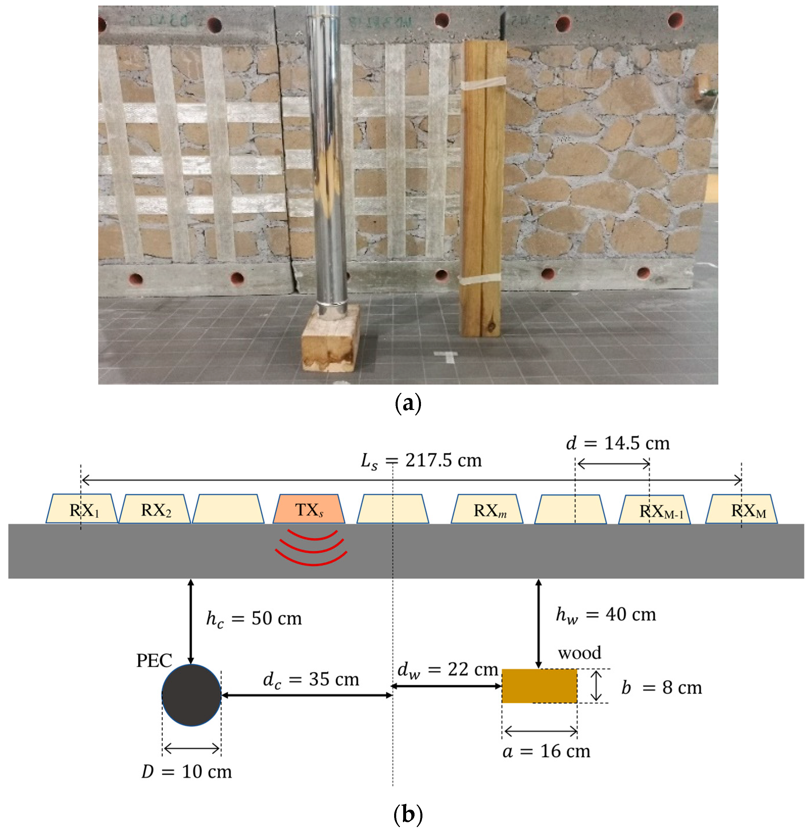
Figure 3 shows a picture (
Figure 3a) and a schematic diagram (
Figure 3b) of the measurement setup. In this first target configuration, a single metallic object is located behind the wall (denoted by the black circle in
Figure 3b). In particular, a circular cylinder of diameter
has been positioned at a distance of
from the wall, with an offset of 19 cm from the center of the probing line.
Such a target has been chosen since the high reflectivity of the metallic cylinder may be representative of very high-scattering objects that may be present in the scenario (e.g., metallic poles), as well as, although in an approximate way as often done in the TWI literature, of a human target, due to its significant dielectric contrast with respect to the background medium. The arrangement of the TX (yellow boxes) and RX (orange box) antennas is also schematically shown in
Figure 3b for the generic
-th view. In order to evaluate the effect of the number of frequencies used in the inversion procedure, the number
of frequency samples extracted from the Fourier transform has been varied between 3 and 41. The frequency range has been kept constant and equal to
.
Figure 4a–c show the behavior of the estimated coordinates of the target center and its diameter extracted from the reconstructed images versus the number of frequencies. Such values are found by setting a threshold of 1/3 on the normalized reconstructed distribution of
and by searching for the minimum circle enclosing the pixels over such a value in a square region of side 30 cm around the actual target location. In particular, both the results obtained by considering the hybrid approach and the TSVD method alone are reported. As can be seen, in almost all cases, the position of the target is correctly estimated. However, the dimension found using the TSVD method alone is always overestimated. Moreover, the hybrid method allows obtaining good results even when using a significantly lower number of frequencies (i.e., higher than 5). Finally, the signal-to-clutter ratio (SCR) of the retrieved images of the inspected scenario, defined as [
55]
has also been computed and shown in
Figure 4d.
As can be seen, the proposed hybrid approach allows obtaining images significantly cleaner than those of the TSVD method alone (the difference between the SCR for the two approaches is almost always higher than 20 dB). Moreover, this graph suggests that a number of frequencies greater than about 20 is sufficient to achieve the best reconstruction quality, since increasing does not result in a higher SCR.
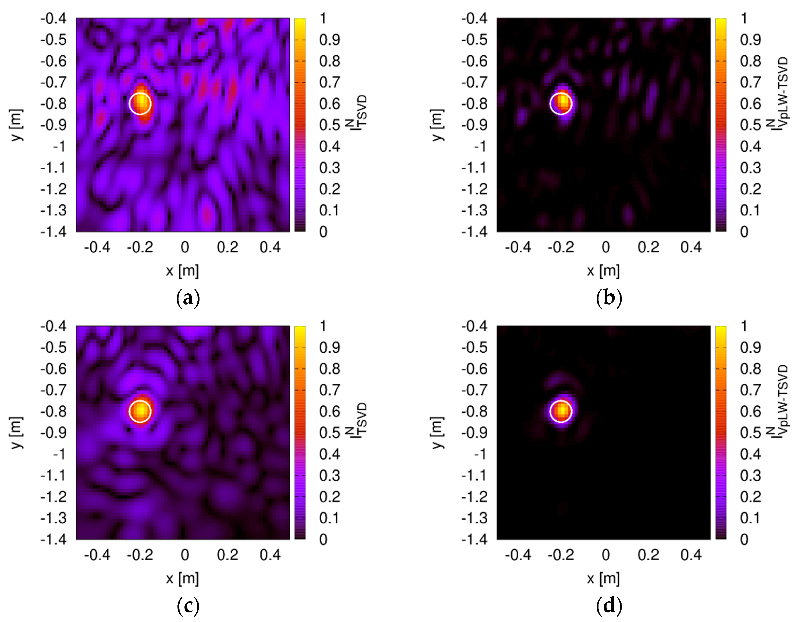
Such results are also confirmed by the normalized images of the retrieved distribution of
, i.e.,
, shown in
Figure 5. Indeed, when only
frequencies are considered, the TSVD image is characterized by significant artifacts and the dimension of the object is slightly overestimated (especially in the vertical direction). Nevertheless, the hybrid approach is able to provide a quite good reconstruction, almost free of artifacts. Increasing the number of frequencies (as in
Figure 5c,d, where
) leads to a better initial estimation with the TSVD method, which in turn results in a clean final image, where the target can be clearly identified and whose dimensions are correctly estimated.
Finally, the effects on the reconstruction capabilities of the number of subdomains used to discretize the investigation area, and consequently of the size
of each pixel of the image, have been evaluated in the case
. In particular,
has been varied between 400 and 10,000 (corresponding to
m). The obtained results, which are summarized in
Table 1, show that the developed approach is quite stable with respect to such a parameter. Indeed, the diameter is almost always estimated correctly. A similar behavior is also shown by the estimated center (not reported for sake of brevity). Moreover, the SCR slightly increases with
.
Such considerations are also confirmed by the examples of reconstructed images shown in
Figure 6. When
is low (e.g.,
), the pixels are large and, thus, do not allow an exact shaping of the target, although its position and dimensions are close to the actual ones. Moreover, an artifact is present above the target. When
is increased, the reconstruction quality improves, allowing a better identification of the shape of the target.
For completeness,
Table 1 also reports the computational times required for running the inversion code on a standard laptop PC equipped with an Intel Core i5-8265U @ 1.60 GHz CPU with 16 GB of RAM. It is worth remarking that, once the scenario is defined, the matrix
and its singular value decomposition can be computed once for all and offline. Consequently, in the table, the time dedicated to such a precomputing step has been separated from the online time necessary to actually perform the inversion. Moreover, since the TSVD and VpLW steps of the inversion procedure rely upon the use of the same matrix
, it can be computed just one time and reused in both stages, allowing an increase in the computational efficiency of the method. Such a consideration is confirmed by the online times shown in
Table 1. Indeed, since all the necessary quantities are precomputed, the TSVD inversion in (7) requires a negligible time, whereas the VpLW step requires approximately 1 s.
3.2. Metallic and Dielectric Targets
As a second configuration, a more challenging scenario, in which two separate targets are located behind the wall, has been considered.
Figure 7 shows a picture and a schematic representation of the considered scenario. In particular, the first target is the same metallic cylinder considered in the previous section (i.e., with diameter
and at distance of
from the wall) but with an increased offset
from the center of the probing line. The second object (schematized by the brown rectangle in
Figure 7b) is a low scattering rectangular cylinder made of wood with sides
and
, which is located at a distance
from the wall with an offset
from the center.
The choice of the wood cylinder, with its low dielectric permittivity, allows checking the effectiveness of the technique in the detection of weak scatterers, especially when interacting with stronger scatterers, as in the considered layout. This is representative of practical challenging TW environments, where the target of the survey must be discriminated from other scatterers and pieces of furniture. The arrangement of the antennas is the same as in the previous case, as schematized in
Figure 7b.
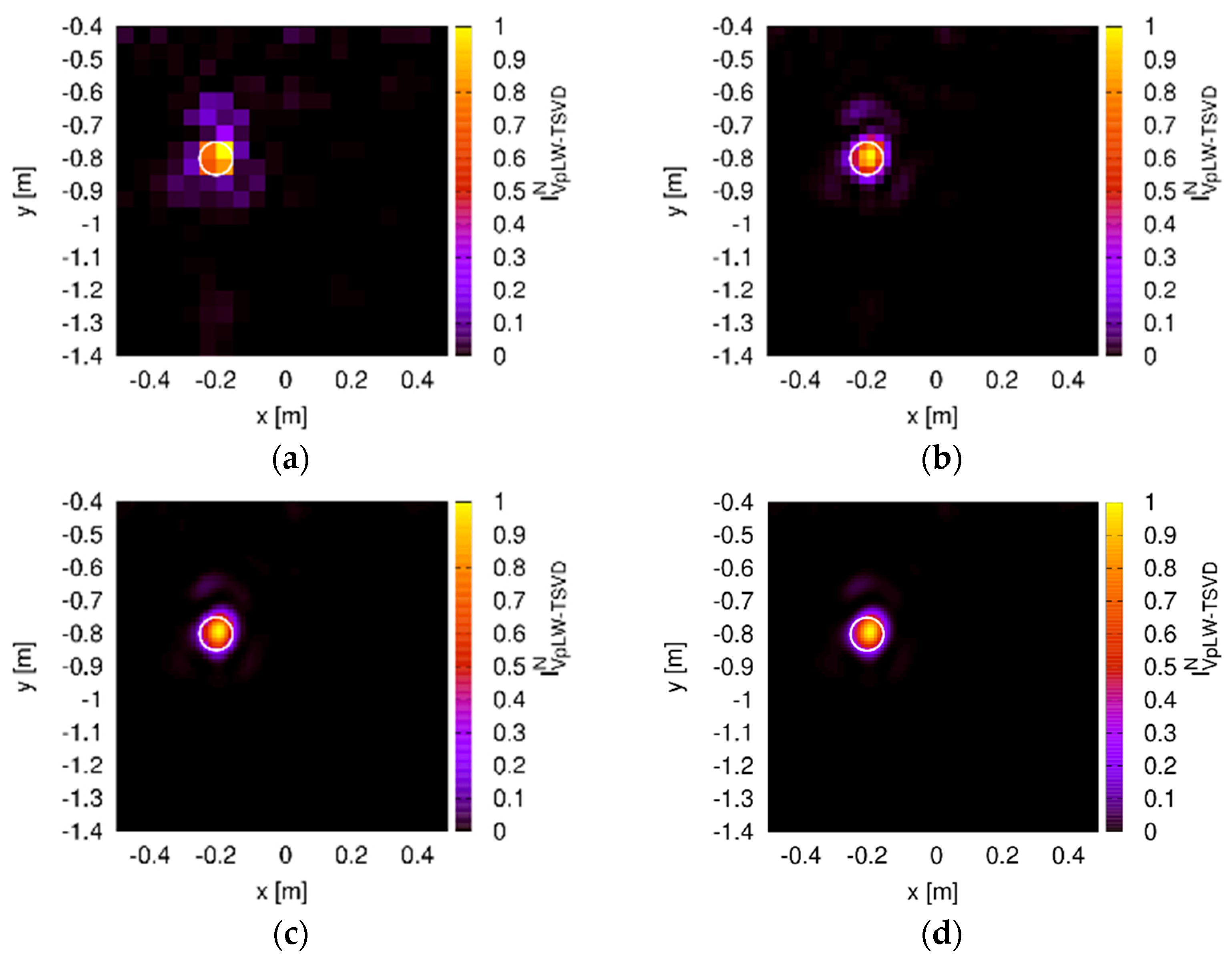
The retrieved normalized distribution of
is shown in
Figure 8. In particular,
Figure 8a reports the results obtained by the TSVD method alone, whereas the final reconstruction provided by the hybrid method is given in
Figure 8b. As can be seen, the initial TSVD image already allows identifying the metallic cylinder. However, significant artifacts are present in the background. Moreover, the wood object cannot be readily seen, since the amplitude of its contribution is comparable to the background noise. However, the application of the hybrid technique greatly enhances the quality of the final image. Indeed, the background is completely free from artifacts, the metallic cylinder is correctly localized and sized, and the low-scattering wood object can be distinguished, although with a lower amplitude.
This fact is confirmed by the values of the SCR: for the TSVD alone it is equal to 22, whereas when considering the hybrid approach it increases to 46.3. In order to better analyze this last result, zooms on the left and right parts of the image are provided in
Figure 8c,d (with the color scale adapted to the respective maximum amplitudes). Now the wood target can be clearly identified in
Figure 8c, and its amplitude is significantly higher than the small artifacts that can be seen in the image.
The results obtained by conventional DAS beamforming techniques [
7,
56,
57,
58] are also shown in
Figure 9 for comparison purposes. In particular, two cases have been considered. In the first one (
Figure 9a), a standard free-space approach, in which the effects of the wall are neglected, is adopted. As expected, the resulting image is totally unfocused and the targets cannot be even identified. Things get better if the wall is properly compensated (
Figure 9b). In this case, the delays used in the beamforming process are computed by taking into account the propagation through the wall by exploiting the Fermat’s principle. As can be seen, the beamforming results are now similar to the ones provided by the TSVD approach alone, although the weaker target has a lower amplitude and the dimension of the PEC cylinder is larger. However, it should be noted that now a different (and approximate) propagation model is used: this does not allow reusing the same matrix already computed for the VpLW method. In particular, for every focusing point, it is necessary to solve a time-consuming optimization problem to find the shortest electrical path of the Fermat’s principle.


 ,
, 


