Methodology for the Definition of Durum Wheat Yield Homogeneous Zones by Using Satellite Spectral Indices

Abstract

One of the main questions facing precision agriculture is the evaluation of different algorithms for the delineation of homogeneous management zones. In the present study, a new approach based on the use of time series of satellite imagery, collected during two consecutive growing seasons, was proposed. Texture analysis performed using the Gray-Level Co-Occurrence Matrix (GLCM) was used to integrate and correct the sum of the vegetation indices maps (NDVI and MCARI2) and define the homogenous productivity zones on ten durum wheat fields in southern Italy. The homogenous zones identified through the method that integrates the GLCM indices with the spectral indices studied showed a greater accuracy (0.18–0.22 Mg ha⁻¹ for ∑NDVIs + GLCM and 0.05–0.49 Mg ha⁻¹ for ∑MCARI2s + GLCM) with respect to the methods that considered only the sum of the indices. Best results were also obtained with respect to the homogeneous zones derived by using yield maps of the previous year or vegetation indices acquired in a single day. Therefore, the survey methods based on the data collected over the entire study period provided the best results in terms of estimated yield; the addition of clustering analysis performed with the GLCM method allowed to further improve the accuracy of the estimate and better define homogeneous productivity zones of durum wheat fields.

1. Introduction

Durum wheat (Triticum turgidum ssp. durum Desf.) is the main raw material for making pasta and is cultivated primarily in the Mediterranean basin, under rainfed conditions, where the unpredictable seasonal rainfall has a decisive influence on the yield and grain quality [1,2]. Another important source of uncertainty in crop production is represented by within-field variability of soil physical and chemical properties that should be taken into account in the management of the crop [3]. A key challenge that wheat growers face is to increase and stabilize the yield and quality attributes over the years, managing the soil spatial variability and, achieving the standards determined by the pasta industry, particularly high grain protein content. In fact, given significant inter- and intra-field variation of agronomic attributes, conventional agricultural systems have limited capacity to respond to the industry demands for increasingly grain quality specifications. The uniform application of inputs such as fertilizer potentially could result in the farmer failing to reach the qualitive standards, as nitrogen application in some areas of the field may not have had the desired effect.

To achieve this goal, Precision Agriculture (PA) techniques, based on the identification of homogeneous management zones within a field, allow the site-specific application of agrochemicals (i.e., definition of optimal sowing rates, fertilization, and fungicide/insecticide applications) and managing spatial-temporal variability of soil properties for crop growth [4].

Crop yield data has been considered the most important parameter for efficiently defining management zones in annual cropping systems [5,6]. In fact, yield mapping is one of the most widely used PA techniques to identify homogeneous zones, for its easy applicability [7]. The identification of areas of similar yield potential, called “productivity zones”, could improve durum wheat performances as some key management decisions are dependent on reliable estimates of expected yield [8].

Productivity zones have most commonly been derived from an analysis of a single yield map but, promising results have been reported by using several years of yield data to create homogeneous management zones. Diacono et al. [9] noted that if an analysis averages yield maps across wet and dry years, then the procedure may neutralize information needed to better understand the interaction between soil properties and climate and the resulting effects on durum wheat yield and grain quality. Therefore, the stability of such zones needs to be tested for each individual field. Ideally, the variability within homogeneous is expected to be uniform spatially and stable across the years, representing a comparable level of yield potential, plant biomass, and/or soil quality [10].

Static soil properties and topographic variables have also been used to derive productivity zones. When compared to the use of multiple years yield maps, deriving productivity zones from soil and topographic information represents a tremendous time savings and is, therefore, appealing to producers [11]. For this reason, although yield mapping represents a useful decision support system for defining homogeneous management zones, it is currently used in combination with soil attributes [11], electrical conductivity crop measurements [12], and remotely sensed images [3].

The use of unmanned aerial vehicles (UAV) [13] and satellite imagery [14] has accelerated the development of new automatic land delimitation tools for recognizing homogeneous zones at field level, since reflectance data and vegetation indices (VIs) are good predictors of crop parameters (e.g., leaf area index, below-ground biomass accumulation nitrogen content) and yields [15,16,17,18].

With reference to the use of remote sensing data, numerous studies have attempted to understand the optimal period for NDVI acquisition for better evaluation and/or definition of homogeneous zones from an agronomic point of view [19]. However, several authors have reported inconsistent advantages for this yield prediction strategy and identification of homogeneous zones [20]. Spatial patterns in yield tend to change from year to year [21], mostly because static soil properties interact differently with meteorological factors and agronomic management [22]. The use of satellite imagery allows the identification of the within-field variability of crop development and yield, albeit with a very high resolution (10 × 10 m), and the definition of homogeneous management zones [23,24], the use of which is limited to the ongoing growing season.

Besides this, another of the main questions facing PA is the evaluation of different algorithms for the delineation of management zones. Before generating variable-rate application maps, in fact, it is necessary to quantify the within-field variability, with the available attributes, i.e., soil chemical or physical criteria, yield, vegetation indices, with spatial statistical indices. Recently, Leroux and Tisseyre [25] provided an extensive review of the methods to assess within-field variability. Researchers have proposed various techniques and algorithms for identifying homogeneous zones, including expert systems [26], segmentation algorithms [27], clustering [28,29], fuzzy algorithms [30,31], and machine learning techniques [32]. The objective of each method is to minimize statistically the within-group variability while maximizing the among-group variability to produce homogeneous groups that are definite from one another. Guastaferro et al. [33] compared different algorithms for the delineation of management zones and outlined the pros and cons for each method. In particular, studies have suggested that vegetation indices extracted from a single pixel, mainly for high-density crops, have a poor ability to describe the canopy structure [34]. For example, NDVI is sensitive for lower LAI values (<3) but is saturated for medium or higher LAI values (>3) [35] with a direct consequence on the definition of homogeneous management zones. Texture analysis, instead, provides the images with additional information reflecting the variation of vegetation structure [33,36]. Recently, texture features extracted from Gray Level Co-Occurrence Matrix (GLCM) [37] were widely used in classification research showing, improved classification accuracy [38] and a better LAI and biomass estimation [39,40].

In light of these motivations, a new approach for delineating homogeneous productivity zones by using satellite spectral indices was proposed. The aim of the study was to identify a methodology, based on a time series of high-resolution observations from satellites of two vegetation index (Normalized Difference Vegetation Index, NDVI and Modified Chlorophyll Absorption in Reflectance Index 2, MCARI2), to reduce the inter-annual effects of weather conditions that normally affect yield monitor-based and/or single-day vegetation index-based maps.

The maps obtained from the time series were processed for texture analysis using the GLCM and, the dataset was elaborated with principal component and cluster analysis for the delineation of homogeneous durum wheat productivity zones.

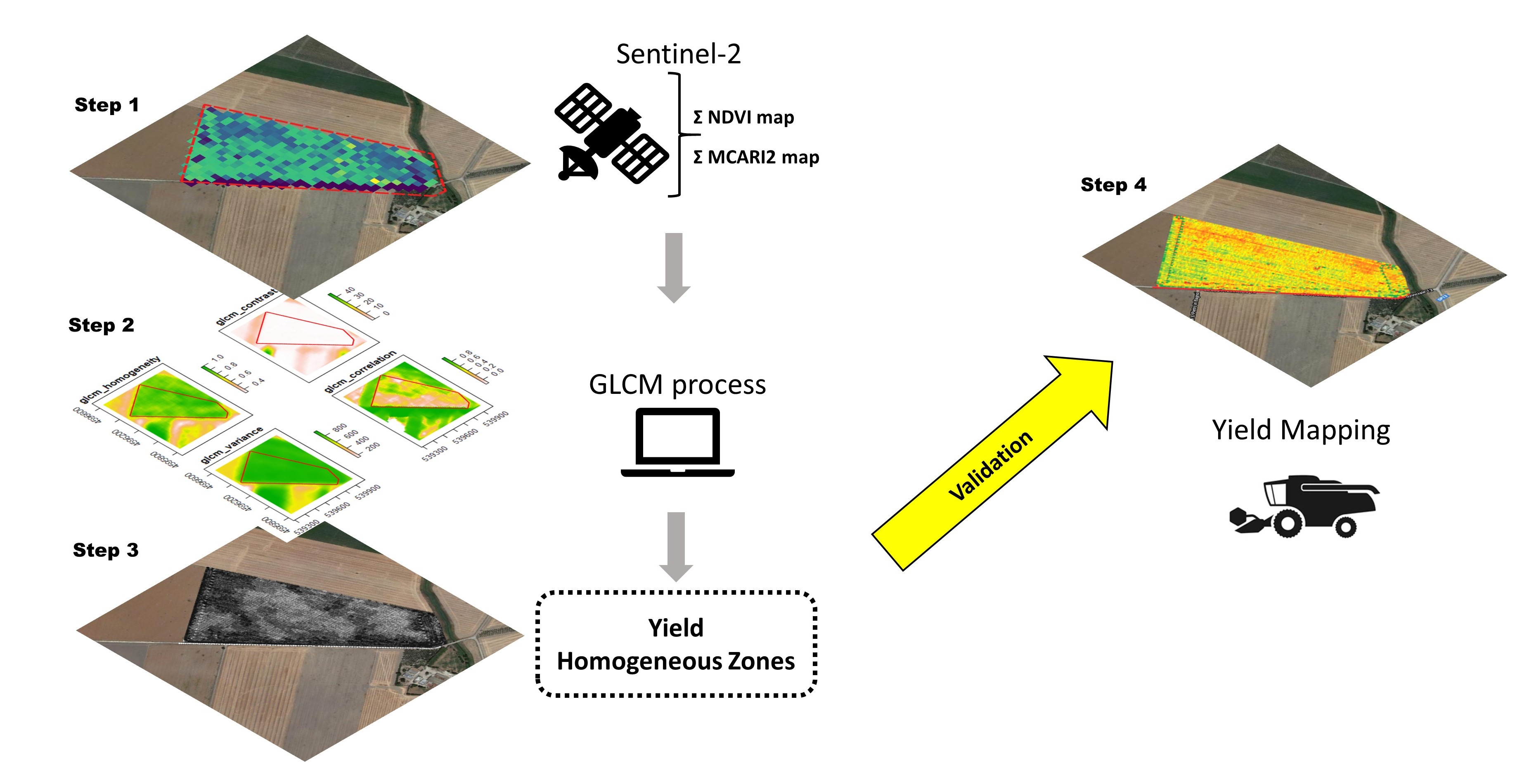
2. Materials and Methods

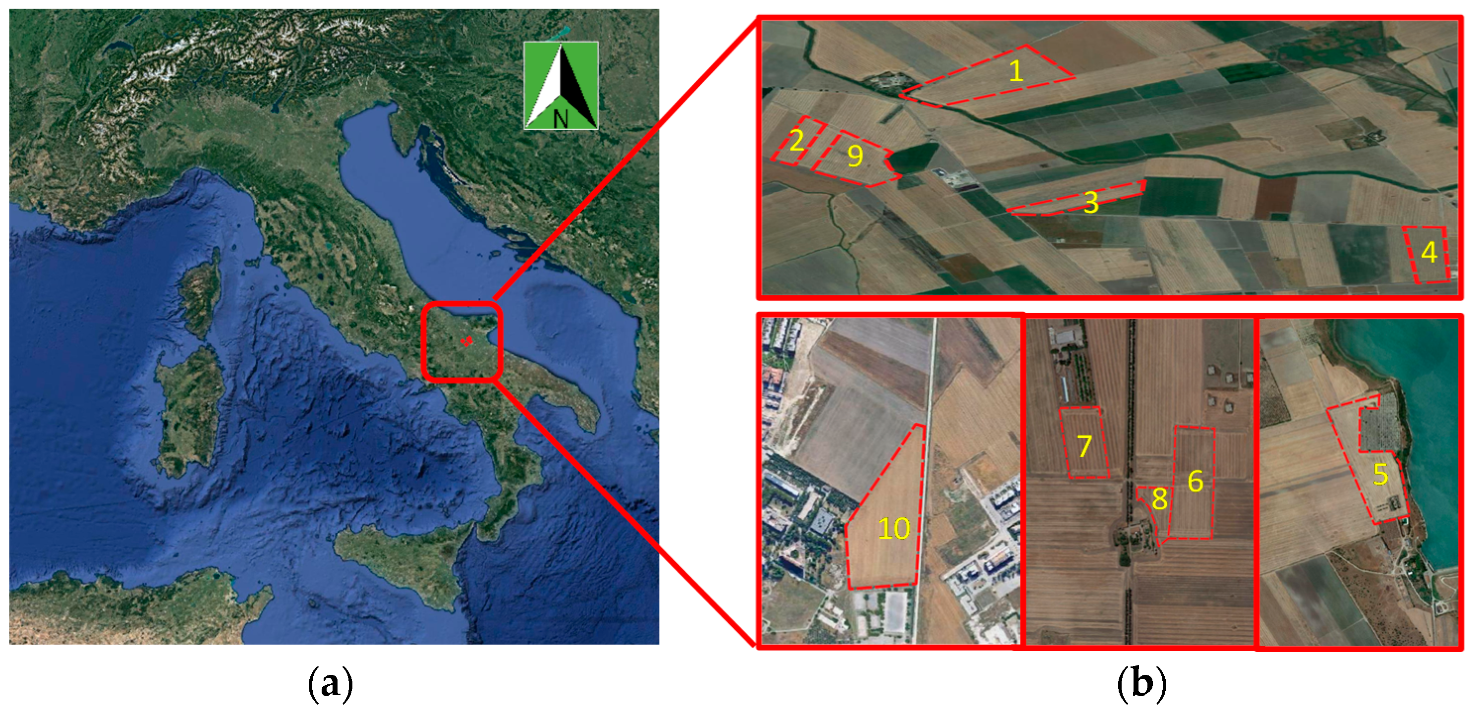
2.1. Study Site

Ten fields extended over a total area of 80 hectares were identified in southern Italy (Figure 1), near the CREA Research Centre for Cereal and Industrial Crops in Foggia (41°28′ N, 15°32′ E, and 75 m asl), which are representative of one of the most important durum wheat cultivated areas in the Mediterranean basin.

The soils in the study area were cultivated with durum wheat for grain production for two consecutive growing seasons. The harvest took place in June 2018 and 2019 and the same crop management was applied in each season. Wheat was grown on the same land, including in 2017, while during the summer between 2018 and 2019, the fields were not cultivated.

The fields are placed in a flat area called ‘Apulian Tavoliere’ and the soil is a silty-clay Vertisol of alluvial origin classified as Fine Mesic Typic Chromoxerert by Soil Taxonomy USDA [41]. The main physical and chemical characteristics of the soil were: 36% clay, 17% silt, and 47% sand; pH 7.8; 17.3 g kg⁻¹ C organic; 1.5 g kg⁻¹ N total; 19 mg kg⁻¹ available P; 111 mg kg⁻¹ interchangeable K. Before sowing, the soil was ploughed and then harrowed for an adequate seed-bed preparation. The sowing period was in the first 10 days of December in both seasons and, the sowing density was 350 seeds m⁻². In both years, nitrogen and phosphorus were applied at a dose of 80 and 70 kg ha⁻¹, respectively. The nitrogen fertilizer was applied in two phases: 1/3 at the sowing date (150 kg ha⁻¹ of bi-ammonium phosphate N 18%, P 46%) and 2/3 at the stem elongation stage (200 kg ha⁻¹ of ammonium nitrate N 26–27%). Weeds during the growing seasons were controlled with the following herbicides: Tralcoximim (1.7 L ha⁻¹) + Clopiralid + MCPA + Fluroxypyr (2.0–2.5 L ha⁻¹).

2.2. Homogeneous Zones Definition

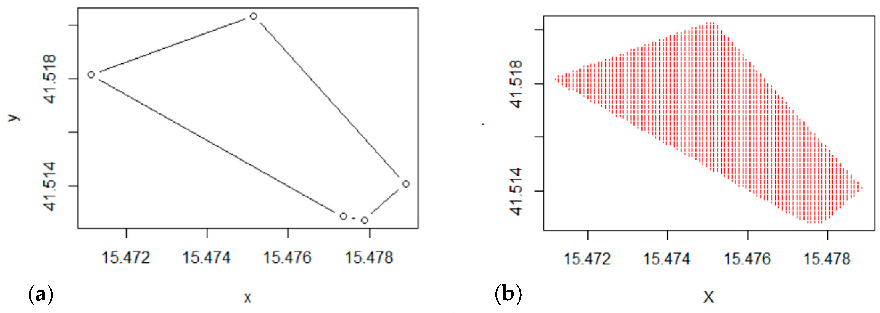
2.2.1. Yield Monitor-Based Maps

The yield map of each field during the two seasons were collected by a combine harvester equipped with a yield-monitoring system (StarFire3000, John Deere, Moline, IL, USA). The high-accuracy GPS technology of the harvester, coupled with on-board yield monitors, allowed accurate and fine-resolution mapping of within-field variation of crop yields. High resolution data collected by the combine harvesters were used to obtain detailed yield shapefiles that were processed by R software for geostatistical analysis. The yield maps, after being processed with R, were elaborated to eliminate the outliers according to the method indicated by Còrdoba et al. [42].

2.2.2. Satellite Data

During durum wheat cultivation, from the moment in which the crop was significantly visible from the satellite and up to the harvest (from 20/01/2018 to 16/06/2018 and from 26/01/2019 to 18/06/2019 for the two growing-seasons, respectively), the reflection bands of the available spectra were extracted from the ESA (European Space Agency—https://sentinel.esa.int/web/sentinel/sentinel-data-access, accessed on 13 April 2021) website.

Table 1. Spectral bands available from Sentinel 2 satellites.

Sensor	Band Name	Sentinel-2A		Sentinel-2B		Resolution (Meters)
		Central Wavelength (nm)	Bandwidth (nm)	Central Wavelength (nm)	Bandwidth (nm)
Multispectral	NIR	835.1	115	833	115	10
Multispectral	Red	664.5	30	665	30	10
Multispectral	Green	560.0	35	559	35	10

reports the characteristics of the spectral bands detected by Sentinel-2A and Sentinel-2B satellites.

The data, obtained and ortho-corrected by ESA, were processed through R software, using the sen2r function of the “sen2r” package, and satellites 2A and 2B were set as sources. Level-2A processing includes scene classification and atmospheric correction applied to Top-Of-Atmosphere (TOA) level 1C ortho imaging products. The resolution of the bands required was 10 × 10 meters.

From the bands obtained, Red (R, σ = ~665 nm), Green (G, σ = ~560 nm), Vegetation Red Edge (VRE, σ = ~780 nm), and a NIR (Near Infra-Red, σ = ~833 nm) were selected, and for each pixel of the maps the spectral indices NDVI (Normalized Difference Vegetation Index) were defined by the Formula (1):

$$NDVI=\frac{NIR-Red}{NIR+Red}$$

(1)

and MCARI2 (Modified Chlorophyll Absorption in Reflectance Index 2), was calculated by the Formula (2):

$$MCARI2=\frac{1.5\left[2.5\left(NIR-Red\right)-1.3\left(NIR-Green\right)\right]}{\sqrt{{\left(2NIR+1\right)}^2-(6 NIR-5\sqrt{Red})-0.5}}$$

(2)

The two indices were selected for their high capacity to detect the homogeneity of the photosynthetic activity of crops [43,44]. In particular, the NDVI was chosen because of the wealth of information and its validation history and the MCARI2 index because it is one of the best predictors of green leaf area index (LAI) [35,45,46] and incorporates a soil adjustment factor while preserving sensitivity to LAI and resistance to chlorophyll influence. Satellite images were acquired throughout the entire durum wheat growth cycle from the tillering stage (Zadoks Growth Scale, GS 31) to harvest (GS 89) [47]. They were then checked and only those in which there was no cloud formation over the fields were used. Therefore, from the 24 maps of 2018 and the 26 maps obtained in 2019, only 14 maps were selected for processing in 2018 and 13 in 2019.

Considering that the NDVI can be affected by the environmental brightness and by the inclination of the incident ray, the sum of vegetation indices (ΣNDVI and ΣMCARI2) were calculated over the observation period (January–June) on each coordinate of the fields. This methodology was used to attribute the same amount of error to all points, while maintaining the effect of each single acquisition date.

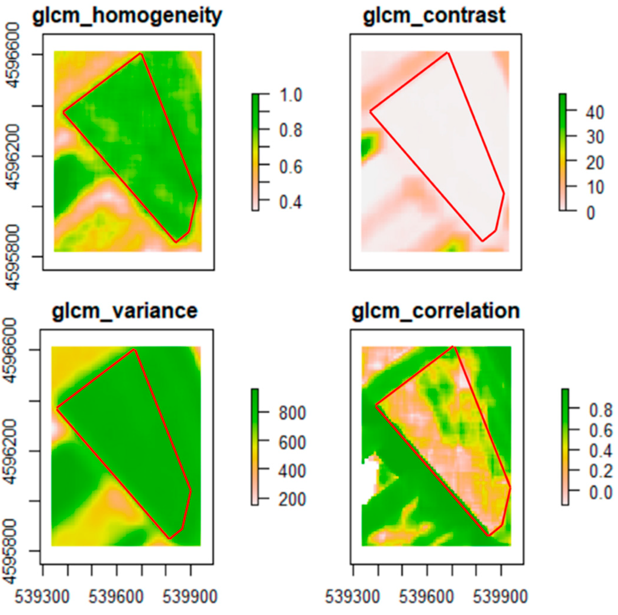
2.2.3. Texture Analysis

The maps obtained from the time series were then processed for the calculation of the GLCM indices developed by Robert Haralick [37] for the characterization of heterogeneous surface samples and inhomogeneity of digital images. Each index highlights a certain texture property, such as homogeneity, irregularity, or contrast. Texture is the term used to characterize the tone of grey-level variations in an image [48]. The construction of GLCM, as reported by Chessel et al. [49], involves first converting an image to greyscale to be discretized in an entire matrix by dividing the range of continuous pixel values into N sub-samples of equal width, called gray levels, the values are then remapped on a single gray level. The elements of GLCM are calculated based on this discretized map by counting the frequency with which, in the matrix, pairs of pixels occur with specific gray levels and in a specified spatial relationship. The adjacency of the pixels can be defined in four different angles: 0, 45, 90, and 135 degrees. The GLCM is then normalized to make the sum of all elements equal to one. Four GLCM indices were selected, and their meanings and formulas are presented in

Table 2. Selected GLCM indices.

Indices	Description	Equation
Homogeneity	Measures image homogeneity. Sensitive to the presence of near diagonal elements in a GLCM, representing the similarity in gray level between adjacent pixels.	${{\displaystyle \sum }}_{i=0}^{N_g-1}{{\displaystyle \sum }}_{j=0}^{N_g-1}\frac{1}{1+{\left(i-j\right)}^2}g\left(i,j\right)$
Contrast	Measures the drastic change in gray level between contiguous pixels. High contrast images feature high spatial frequencies.	${{\displaystyle \sum }}_{i=0}^{N_g-1}{{\displaystyle \sum }}_{j=0}^{N_g-1}{\left(i-j\right)}^2{g}^2\left(i,j\right)$
Variance	A measure of heterogeneity, variance increases when the gray level values differ from their mean.	${{\displaystyle \sum }}_{i=0}^{N_g-1}{{\displaystyle \sum }}_{j=0}^{N_g-1}{\left(i-\mu \right)}^{2}g\left(i,j\right)$
Correlation	Measures the linear dependency in the image. High correlation values imply a linear relationship between the gray levels of adjacent pixel pairs.	${{\displaystyle \sum }}_{i=0}^{N_g-1}{{\displaystyle \sum }}_{j=0}^{N_g-1}\left(i-\mu \right)\left(j-\mu \right)g\frac{\left(i,j\right)}{{\sigma }^2}$

Note: Ng is the number of gray levels, g(i,j) is the entry (i,j) in the GLCM, µ is the GLCM mean, and σ² is the GLCM variance. Source: [36].

.

For each field, a regular grid of points identified by their geographical coordinates was prepared, with a layout of 3 × 3 m (Figure 2). The map projection was converted from WGS84 to the UTM projection system to express the distances in physical units (meters). Therefore, the distances between the sites within the field can be expressed as absolute distances (meters) instead of relative distances (degrees), facilitating interpretation. For this operation, we used the spTransform function of the “rgdal” package [50] which converts the geographic coordinates to UTM Cartesian coordinates.

The extract function of the “raster” package was used to extract the corresponding values from the raster of the spectral indices NDVI and MCARI2 and the glcm function of the homonymous package, to calculate the respective GLCM indices. These functions allowed to obtain a data frame in which in each row a point of the map (long, lat) was described with a column for the spectral index and a column for each GLCM index, for each date of the observed period.

The values of the spectral indices of all the dates of the two periods were added for each point, while for the GLCM indices, the maximum value reached in the observation period was used. So, the new data frame, which still had the coordinates of the points of the regular grid in each row, had the sum of the spectral index (Σ) values in the columns and a column for each GLCM index represented by the maximum value collected in the period.

2.2.4. Modelling Analysis

The dataset was used for Principal Component Analysis (PCA), to verify any correlations between the variables and to observe the effect of each variable on the distribution of points. In recent years, PCA has been extensively used in remote sensing classification developments, especially for hyperspectral imagery [32]. Principal Component Analysis was carried out for the study of clustering methods, taking into consideration the percentage of variance explained by the first and second components and therefore considering the loadings of the methods observed on the two components as suggested by Deur et al. [32].

The same dataset of the PCA was subjected to fuzzy k-means cluster analysis [51] for homogeneous zones identification, which allows the division of a set of objects into k groups based on their attributes, assuming that the attributes of the objects can be represented as vectors, thus forming a vector space. The goal of the algorithm was to minimize the total intra-group variance. Consequently, each group was identified by a centroid or midpoint. The algorithm worked iteratively to assign each coordinate of the fields to one of the k groups based on the features that were provided. Initially, it created k partitions and assigned the coordinates of the fields to each partition and calculated the centroid of each group. Later, it built a new partition associating each coordinate to the group whose centroid was closest to it. Finally, the centroids were recalculated for the new groups, until the algorithm converged. The variables that were observed for the development of PCA and k-means clustering are shown in

Table 3. Variables observed in the developed PCA and clustering analysis on studied models.

Models	Variables
∑NDVI	∑NDVI by 1 year; Year; Standard deviation of NDVI by 1 year
∑MCARI2	∑MCARI2 by 1 year; Year; Standard deviation of MCARI2 by 1 year
NDVI single-day	NDVI of a single day; Year
MCARI2 single-day	MCARI2 of a single day; Year
∑NDVI +GLCM	∑NDVI by 1 year; Year; Standard deviation of NDVI by 1 year; GLCM (Homogeneity, Contrast, Variance, Correlation)
∑MCARI2 +GLCM	∑MCARI2 by 1 year; Year; Standard deviation of MCARI2 by 1 year; GLCM (Homogeneity, Contrast, Variance, Correlation)

.

The methods were then considered in the process of attributing to clusters, in which the Euclidean distance was the similarity distance included in the classification algorithm optimization function. Fuzzy clustering of spatial components in this space was achieved by setting a fuzziness weighting exponent to 1.3, as indicated in PA applications [33,52,53]. The cluster analysis, as indicated in the protocol proposed by Cordoba et al. [42], was calculated using the “e1071” package [54]. A summary index was calculated to determine the optimal number of k-classes [55,56,57,58].

2.2.5. Yield Maps Elaboration

For each clustering model, each point of the field, identified by its coordinates, was assigned to a cluster based on its measured values of the variables considered in the model. Then, the sum of the average yield obtained in the two-year period 2018–2019 of each point belonging to a cluster was performed, then was divided by the number of points of the cluster. In this way, the average yield and the relative standard deviations of each cluster were obtained.

Then, the regression between yield obtained from the identified clusters and the clusters identified from the 2019 yield distribution was studied. The regressions were described with R² and Root Mean Square Error (RMSE). This analysis was carried out using the gls function of the “nlme” package [59].

2.3. Comparison Analysis

To confirm the hypothesis of our work, a comparison was made between the mean yield of the homogeneous zones created with clustering based on the sum of the spectral indices in the observed period and that made with the yield data measured at harvest time. The same comparison was also made with clustering performed with the dataset obtained with the vegetation indices and GLCM method. In addition, we compared the homogeneous yield maps derived from our approach proposed in this work, with the homogeneous zones defined on the basis of the yield maps of the previous year and also on the basis of a single-day vegetation index maps (NDVI and MCARI2). In the latter case, the maps generated by the satellite images were collected in the weeks corresponding to the anthesis phenological stage of durum wheat (beginning of May) in both growing seasons. The Tukey test method was used to compare the yield data obtained from the clusters identified by the proposed models (NDVIs + GLCM, NDVIs, MCARI2s + GLCM, and MCARI2s).

3. Results and Discussion

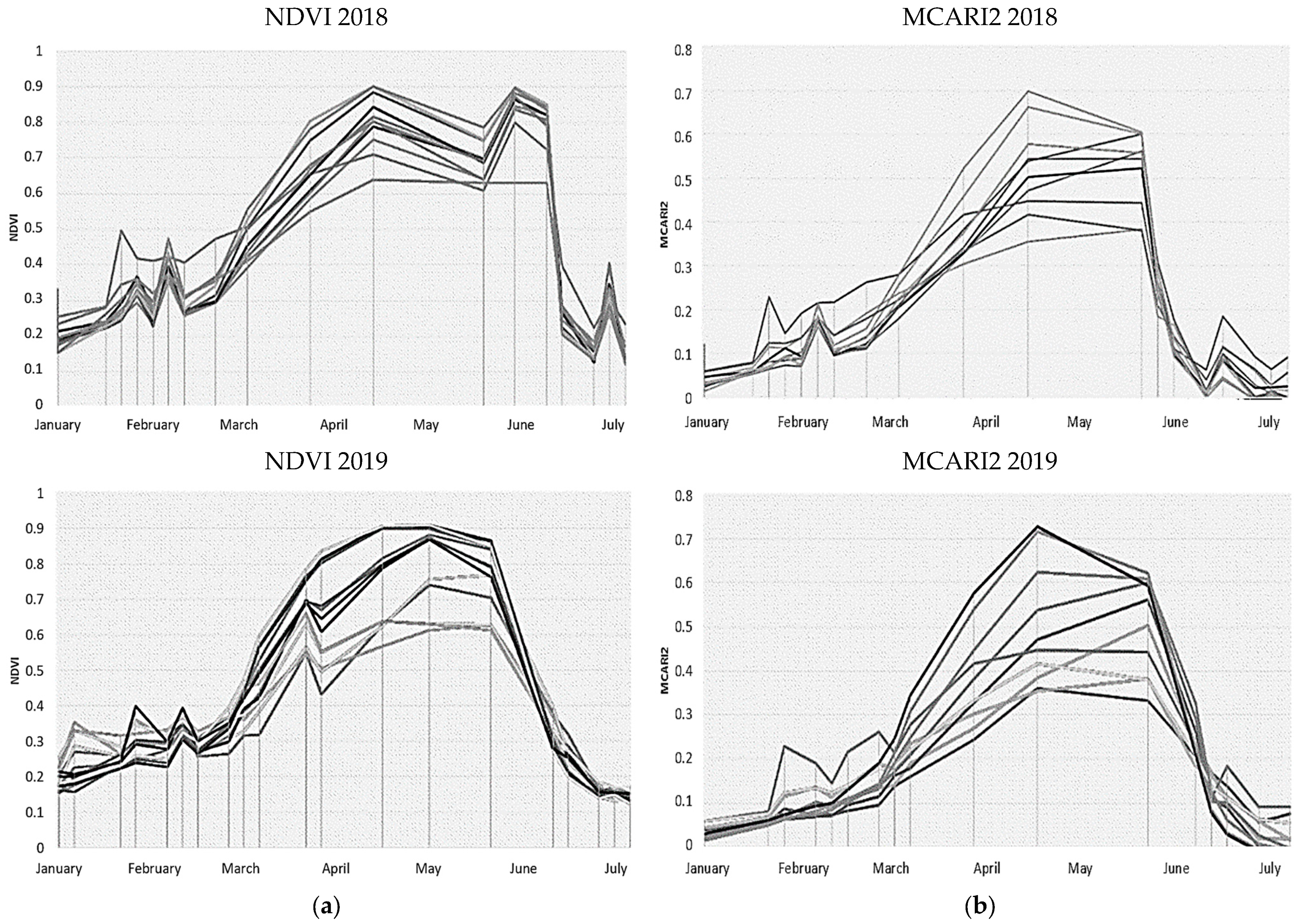
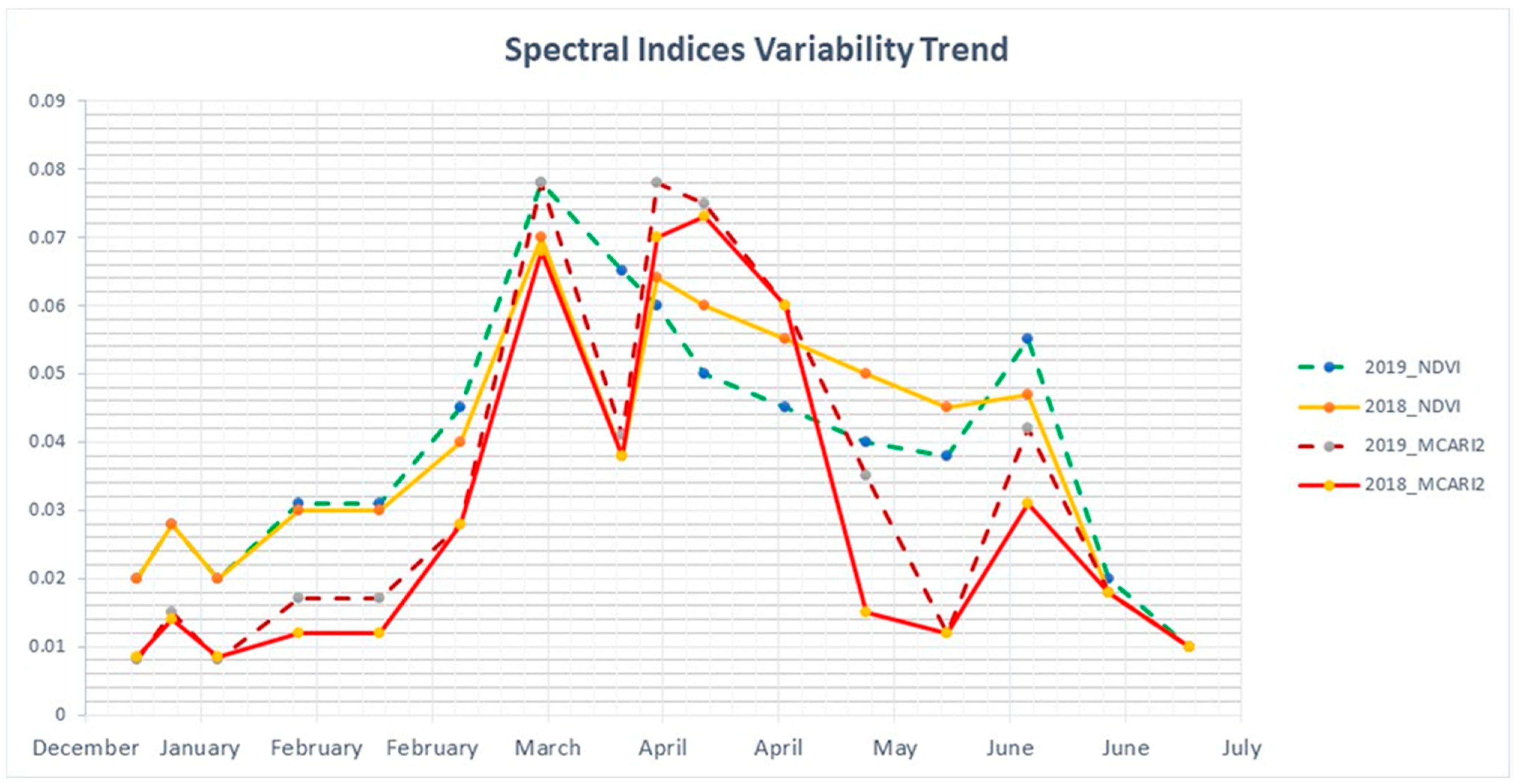
3.1. Vegetation Indices Derived from a Time Series of Satellite Imagery

The results of spectral indices NDVI and MCARI2 were placed in chronological order, covering the entire time span of cultivation curve of durum wheat (Figure 3). The two indices showed the same trend reflecting the crop phenology with an accurate synchronization with the durum wheat growth. In the past, several studies have reported to use of remote sensing for estimating biomass accumulation and predicting crop phenology by analyzing VI time-series data [60]. Currently, interest has shifted to the use accumulated NDVI throughout the wheat growing season with the measurements taken at GS30, GS32, GS37, and GS65 growth stages, which are considered more informative [61]. Zheng et al. [62] selected three key periods (mid-March, mid-April, and mid-May), corresponding to the early, middle, and late wheat growing stages, respectively, to validate the relationship between the satellite imagery and estimated biomass. In our study, the trend of the two vegetation indices showed a high variability during the entire growth cycle of durum wheat in the 10 fields. The variability of the values of the two spectral indices was observed by analyzing the variation of the standard deviation between the values measured on each coordinate, for each observation date over the two years (Figure 4).

The rise of the crop density and the variation of the photosynthetic activity values increased the standard deviation among the measured values. A consistent increase in values for both vegetation indices was observed during the stem elongation phase up to the flowering phase, when the curves reached a plateau, due to the complete coverage of the soil surface, from the end of March to the beginning of May. The MCARI2 index showed a higher standard deviation during this phase than the NDVI index, while during the grain filling period, the NDVI lost sensitivity in the estimation of vegetation cover, resulting in a higher standard deviation than MCARI2. This confirmed a previous study [35] showing the loss of sensitivity of the NDVI for values of LAI greater than 3 and, the greater potential of MCARI 2 for estimating LAI and biomass. The decrease in the values of the vegetation indices at the end of the season was attributed to the senescence of the leaves which increased the reflectance of the red band and decreased the reflectance of the NIR band.

As reported in Figure 5, the acquisition of the satellite image for a single day showed low values of variability (min = 0.008) between coordinates and a high uniformity in the crop, at the same time, it showed high values of variability (max = 0.07) between coordinates and low uniformity in the crop. In

Table 4. Mean values (μ) of the sum of the two spectral indices and standard deviation (σ) collected during 2018 and 2019.

FIELD	ΣNDVI		ΣMCARI2
	μ	σ	μ	σ
1	9.15	0.39	4.11	0.36
2	8.81	0.33	3.96	0.33
3	8.72	0.37	3.88	0.30
4	8.74	0.38	3.88	0.28
5	8.97	0.29	4.05	0.22
6	8.98	0.34	4.05	0.27
7	9.02	0.33	4.09	0.28
8	9.05	0.42	4.03	0.37
9	9.01	0.28	3.99	0.23
10	8.38	0.49	3.56	0.39

, were reported the average values of the two years (2018–2019) of the NDVIs and MCARI2s sum in the 10 fields.

The sum of the mean NDVI values were approximately double those of MCARI2, while the standard deviation for both cumulative indices were comparable, suggesting a greater sensitivity to the variation of the MCARI2 fields compared to the NDVI [63]. Among the ten fields investigated, field 1 was the one with the highest average values for both indices (9.15 and 4.11 for ΣNDVI and ΣMCARI2, respectively), while field 10 showed the lowest average values of sum of the two spectral indices (8.38 and 3.56 for ΣNDVI and ΣMCARI2, respectively). Field 10 was also the one with the highest standard deviation for both vegetation indices.

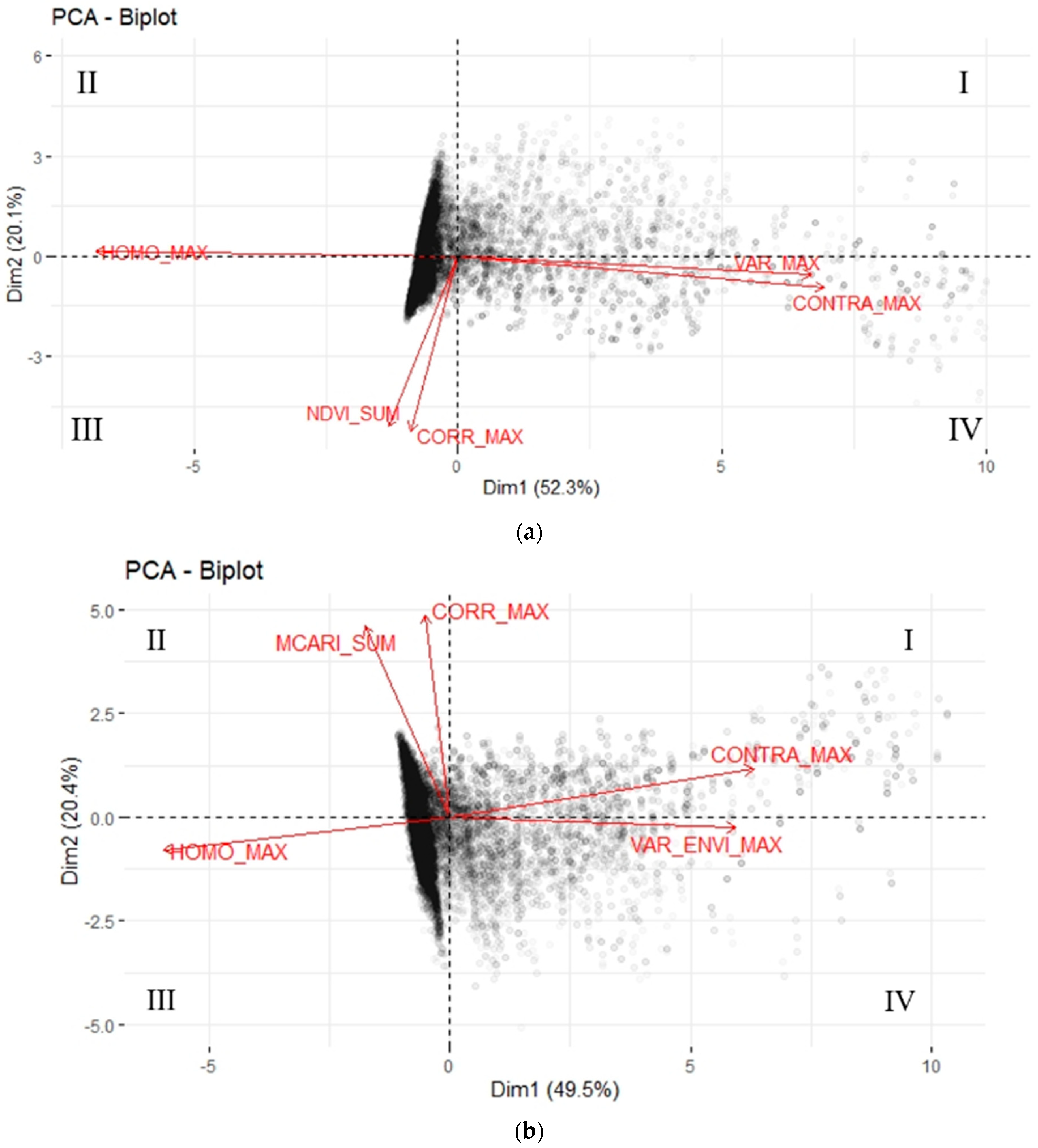
3.2. GLCM Processing and Clustering Analysis

GLCM processing allowed to extract the homogeneity, contrast, variance, and correlation from each pixel constituting the raster of the spectral indices. Then, the results were sorted to form an array containing the coordinates of the grid points in the rows and the dates in the columns. The values were the intensities of the GLCM indices. Therefore, the maximum values of each row were searched, to verify the maximum peak reached by the pixels in the time span of cultivation. As a result, Figure 5 reported the calculation of the four GLCM indices searched for field 1.

The analyzed models showed R² values between 0.621 (RMSE = 1.15) obtained in the model based on the yield map of the previous year and 0.982 (RMSE = 0.25) obtained from the model based on the sum of the NDVI corrected by the GLCM processing. The two models based on the sum of the spectral indices with GLCM showed higher values of R² and lower values of RMSE (

Table 5. Relationship between the averages calculated in the clusters obtained from the models compared with the cluster averages obtained from the yield values.

Model	Regression	R2	RMSE
ΣNDVI+GLCM		0.982	0.25
Σ_NDVI		0.695	1.03
NDVI_Single-day		0.626	1.14
PREV_YEAR		0.621	1.15
ΣMCARI2+GLCM		0.878	0.649
ΣMCARI2		0.676	1.06
MCARI2_Single-day		0.785	0.862

).

The PCA developed on all data from the ten fields, by averaging the two years, showed that the set of observed variables explain 72.1% of the overall variance for the NDVI dataset and 69.96% for the dataset relating to MCARI2 (Figure 6).

Regarding the NDVI, homogeneity (−0.57) and contrast (0.57) showed greater influence on the first component (

Table 6. Loadings of variables processed with the PCA.

	NDVI		MCARI2
FACTORS	PC1 (52.00%)	PC2 (20.10%)	PC1 (49.51%)	PC2 (20.45%)
Spectral_indices_sum	−0.11	0.69	−0.16	0.67
Homogeneity_max	−0.57	−0.02	−0.55	−0.11
Contrast_max	0.58	0.13	0.59	0.17
Variance_max	0.56	0.07	0.55	0.55
Correlation_max	−0.07	0.71	−0.05	0.71

), while correlation (0.66) and NDVI_sum (0.64) showed the greatest influence on the second component. In the case of MCARI2, variance (0.55), homogeneity (−0.55), and contrast (0.59) showed the greatest influence on the first component (Table 6), while the correlation (0.71) and the MCARI2_sum (−0.67) showed the greatest influence on the second component.

The visualization of these results is shown in Figure 6. In the two lower quadrants (III and IV), all the coordinates of the points that showed greater values of the NDVIs during the observation period and a greater GLMC-correlation were concentrated. In the upper quadrants (I and II), all the coordinates of the points that recorded lower values of the NDVIs fell. With the same value of NDVIs and GLMC-correlation, the points were also distributed on the right and left due to greater GLMC-homogeneity and GLMC-contrast, respectively. Similarly, for the MCARI2 index, the PCA analysis showed a biplot with the analogous distribution of both the GLCM indices and the MCARI2 data (Figure 6b). Using the GLCM indices, two, three, and four clusters were evaluated. Based on the calculated indices (

Table 7. Indices used to select the number of clusters from fuzzy k-means cluster results for 10 durum wheat fields, in Italy. For each index, the optimum class number among 2, 3, or 4 classes is suggested by the lowest index value, with a red background.

			NDVI			MCARI2
Field	No. Cluster	2	3	4	2	3	4
1	XieBeni	8.45 × 10−6	7.83 × 10−6	8.32 × 10−6	3.95 × 10−6	3.55 × 10−6	2.44 × 10−6
	FukSug	−1.01 × 105	−1.18 × 105	−1.01 × 105	−1.02 × 105	−2.95 × 105	−1.31 × 105
	PartCoef	1.01 × 10	1.00 × 10	1.06 × 10	1.01 × 10	1.01 × 10	1.02 × 10
	PartEntr	9.94 × 10−2	9.16 × 10−2	9.43 × 10−2	2.15 × 10−2	1.99 × 10−2	3.04 × 10−2
2	XieBeni	7.50 × 10−6	6.61 × 10−6	0.00000769	4.8 × 10−6	2.14 × 10−6	2.26 × 10−6
	FukSug	−1.04 × 105	−1.09 × 105	−1.05 × 105	−3.26 × 105	−1.42 × 105	−4.26 × 105
	PartCoef	1.07 × 10	1.02 × 10	1.08 × 10	1.05 × 10	1.05 × 10	1.09 × 10
	PartEntr	9.20 × 10−2	9.19 × 10−2	9.55 × 10−2	3.56 × 10−2	1.14 × 10−2	1.30 × 10−2
3	XieBeni	8.36 × 10−6	7.37 × 10−6	0.00000819	2.74 × 10−6	2.64 × 10−6	3.85 × 10−6
	FukSug	−1.03 × 105	−1.08 × 105	−1.05 × 105	−2.17 × 105	−4.10 × 105	−5.14 × 105
	PartCoef	1.06 × 10	1.01 × 10	1.03 × 10	1.07 × 10	1.04 × 10	1.06 × 10
	PartEntr	9.96 × 10−2	9.18 × 10−2	9.91 × 10−2	2.73 × 10−2	1.29 × 10−2	3.51 × 10−2
4	XieBeni	9.57 × 10−6	7.82 × 10−6	0.00000898	4.13 × 10−6	3.29 × 10−6	3.82 × 10−6
	FukSug	−1.06 × 105	−1.08 × 105	−1.06 × 105	−3.17 × 105	−1.89 × 105	−4.63 × 105
	PartCoef	1.04 × 10	1.02 × 10	1.01 × 10	1.06 × 10	1.01 × 10	1.03 × 10
	PartEntr	9.77 × 10−2	9.54 × 10−2	9.71 × 10−2	3.32 × 10−2	1.27 × 10−2	3.91 × 10−2
5	XieBeni	7.84 × 10−6	7.86 × 10−6	0.00000789	4.66 × 10−6	4.04 × 10−6	4.43 × 10−6
	FukSug	−1.08 × 105	−1.09 × 105	−1.02 × 105	−4.60 × 105	−1.79 × 105	−2.69 × 105
	PartCoef	1.04 × 10	1.03 × 10	1.05 × 10	1.07 × 10	1.01 × 10	1.10 × 10
	PartEntr	9.57 × 10−2	9.20 × 10−2	9.60 × 10−2	3.06 × 10−2	1.37 × 10−2	2.01 × 10−2
6	XieBeni	8.3 × 10−6	8.02 × 10−6	0.00000903	2.35 × 10−6	2.01 × 10−6	3.01 × 10−6
	FukSug	−1.01 × 105	−1.07 × 105	−1.05 × 105	−3.69 × 105	−1.56 × 105	−2.52 × 105
	PartCoef	1.05 × 10	1.02 × 10	1.04 × 10	1.02 × 10	1.01 × 10	1.08 × 10
	PartEntr	9.20 × 10−2	9.32 × 10−2	9.32 × 10−2	2.79 × 10−2	1.07 × 10−2	1.35 × 10−2
7	XieBeni	8.81 × 10−6	7.96 × 10−6	0.00000874	4.23 × 10−6	2.2 × 10−6	4.49 × 10−6
	FukSug	−1.04 × 105	−1.06 × 105	−1.05 × 105	−3.62 × 105	−3.85 × 105	−4.59 × 105
	PartCoef	1.02 × 10	1.03 × 10	1.08 × 10	1.04 × 10	1.03 × 10	1.09 × 10
	PartEntr	9.73 × 10−2	9.67 × 10−2	9.68 × 10−2	1.89 × 10−2	1.77 × 10−2	3.13 × 10−2
8	XieBeni	7.62 × 10−6	7.17 × 10−6	0.00000928	3.78 × 10−6	2.88 × 10−6	4.22 × 10−6
	FukSug	−1.02 × 105	−1.07 × 105	−1.06 × 105	−3.77 × 105	−3.91 × 105	−3.27 × 105
	PartCoef	1.01 × 10	1.01 × 10	1.09 × 10	1.06 × 10	1.03 × 10	1.09 × 10
	PartEntr	9.81 × 10−2	9.45 × 10−2	9.93 × 10−2	3.96 × 10−2	1.85 × 10−2	3.42 × 10−2
9	XieBeni	8.98 × 10−6	7.94 × 10−6	0.00000995	3.04 × 10−6	2.78 × 10−6	3.73 × 10−6
	FukSug	−1.06 × 105	−1.08 × 105	−1.07 × 105	−3.72 × 105	−1.57 × 105	−4.35 × 105
	PartCoef	1.03 × 10	1.03 × 10	1.04 × 10	1.04 × 10	1.01 × 10	1.04 × 10
	PartEntr	9.07 × 10−2	9.01 × 10−2	9.43 × 10−2	3.78 × 10−2	3.29 × 10−2	9.51 × 10−2
10	XieBeni	8.22 × 10−6	7.69 × 10−6	0.00000962	3.52 × 10−6	2.87 × 10−6	3.63 × 10−6
	FukSug	−1.06 × 105	−1.08 × 105	−1.05 × 105	−2.31 × 105	−1.68 × 105	−3.97 × 105
	PartCoef	1.08 × 10	1.01 × 10	1.04 × 10	1.06 × 10	1.05 × 10	1.09 × 10
	PartEntr	9.44 × 10−2	9.42 × 10−2	9.63 × 10−2	2.19 × 10−2	1.45 × 10−2	3.15 × 10−2

), for all fields over two years, the optimal number of clusters (i.e., homogeneous zones) was three, both for the NDVI and for the MCARI2.

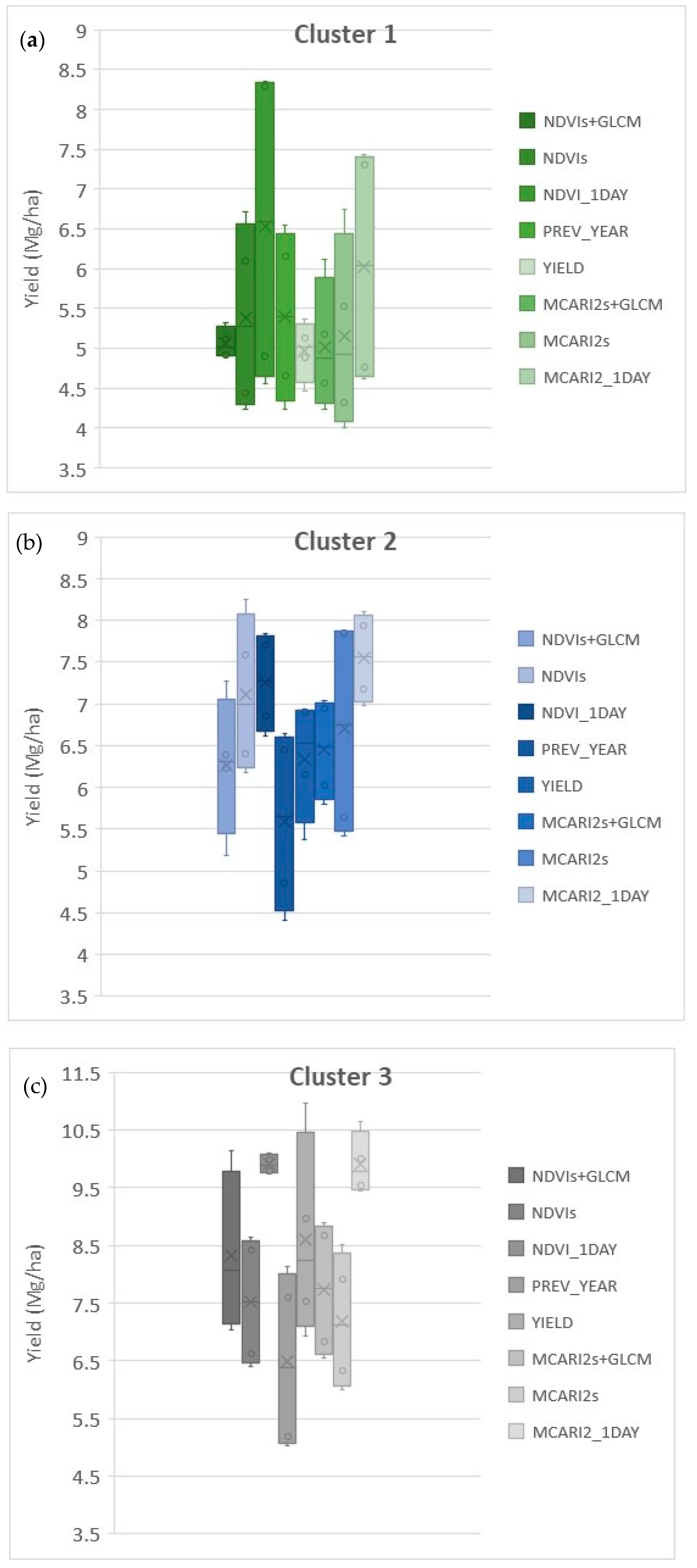
3.3. Comparison of Homogeneous Areas Obtained with Different Methods

Clustering and visualization on the maps based on the NDVIs and MCARI2s values of the entire study period (averaged 2018–2019), integrated with the GLCM indices and compared with 10 yield maps were reported in Supplementary Table S1. The average of the estimated yield values calculated for the three homogeneous zones using the various models proposed (NDVIs + GLCM, NDVIs, MCARI2s + GLCM, MCARI2s, single-day VI, and the yield map of the previous year, 2017) were reported in

Table 8. Average of the two-year estimated values (μ), with standard deviation (σ) and range of the yield values (Mg ha⁻¹) of the areas intercepted by the seven clustering modes in ten fields. Different letters indicate significant differences at Tukey test (p-value < 0.05) between the three clusters of the same field.

FIELD	ZONE	∑NDVI +GLCM	∑NDVI	NDVI Single-Day	Yield Map 2017	Measured Yield	∑MCARI2 +GLCM	∑MCARI2	MCARI2 Single-Day
1	1	5.01a	5.27a	6.42a	5.40a	4.80 ± 0.3	4.87a	4.77a	5.96a
	Δμ%	4.38%	9.79%	33.75%	12.50%		1.46%	−0.63%	24.17%
	2	6.31b	7.33b	7.28a	5.65a	6.53 ± 0.4	6.48b	6.75b	7.56b
	Δμ%	−3.37%	12.25%	10.30%	−13.48%		−0.77%	3.37%	13.62%
	3	8.07c	7.41c	9.89b	6.39b	8.25 ± 0.7	7.76c	6.95c	9.78c
	Δμ%	−2.18%	−10.18%	16.58%	−22.55%		−5.94%	−15.76%	15.64%
2	1	4.53a	4.74a	5.67a	5.11a	4.36 ± 0.3	4.42a	4.39a	5.50a
	Δμ%	3.90%	8.72%	30.05%	17.09%		1.26%	0.57%	26.15%
	2	6.07b	6.74b	6.94b	5.28a	5.98 ± 0.4	6.02b	6.35b	7.11b
	Δμ%	1.51%	12.80%	13.84%	−11.63%		0.75%	6.19%	15.90%
	3	8.28c	7.22b	9.80c	6.52b	8.14 ± 0.7	7.88c	7.24b	9.68c
	Δμ%	1.66%	−11.36%	16.94%	−19.96%		−3.19%	−11.06%	15.87%
3	1	4.52a	4.81a	5.62a	5.11a	4.38 ± 0.2	4.34a	4.40a	5.46a
	Δμ%	3.20%	9.94%	28.34%	16.69%		−0.80%	0.46%	24.80%
	2	5.33b	6.23b	6.36a	5.05a	5.49 ± 0.4	5.54b	5.71b	6.59b
	Δμ%	−2.91%	13.48%	13.61%	−8.11%		0.82%	3.92%	16.69%
	3	7.85c	7.01b	9.22b	6.65b	7.74 ± 0.7	7.63c	6.68c	8.68c
	Δμ%	1.42%	−9.43%	16.01%	−14.08%		−1.49%	−13.76%	10.83%
4	1	4.67a	4.94a	5.72a	5.17a	4.56 ± 0.3	4.59a	4.52a	5.25a
	Δμ%	2.52%	8.34%	25.58%	13.39%		0.77%	−0.88%	15.15%
	2	5.34a	6.22b	6.12a	4.92a	5.53 ± 0.4	5.48b	5.65b	6.26b
	Δμ%	−3.35%	12.49%	9.72%	−10.95%		−0.81%	2.26%	11.74%
	3	7.61b	7.02b	9.18b	6.61b	7.76 ± 0.7	7.54c	6.69c	8.68c
	Δμ%	−1.93%	−9.54%	15.49%	−14.76%		−2.77%	−13.80%	10.61%
5	1	4.80a	5.02a	5.90a	5.27a	4.65 ± 0.4	4.70a	4.60a	5.36a
	Δμ%	3.12%	7.96%	26.88%	13.33%		1.08%	−1.08%	15.16%
	2	5.61b	6.44b	6.29a	5.02a	5.83 ± 0.6	5.78b	6.10b	6.35b
	Δμ%	−3.69%	10.56%	7.39%	−13.91%		−0.86%	4.72%	8.20%
	3	7.91c	7.16b	9.85b	6.49b	8.13 ± 0.9	7.81c	7.15c	9.18c
	Δμ%	−2.71%	−11.88%	17.47%	−20.18%		−3.94%	−12.00%	11.49%
6	1	4.98a	5.15a	6.11a	5.36a	4.79 ± 0.4	4.86a	4.70a	5.50a
	Δμ%	3.97%	7.52%	27.69%	11.91%		1.57%	−1.78%	14.94%
	2	5.80b	6.59b	6.74a	5.18a	5.95 ± 0.7	6.01b	6.13b	6.76b
	Δμ%	−2.44%	10.77%	11.73%	−12.87%		1.01%	3.03%	11.99%
	3	8.18c	7.40b	9.75b	6.63b	8.42 ± 1.1	8.02c	7.19c	9.44c
	Δμ%	−2.85%	−12.06%	13.65%	−21.27%		−4.75%	−14.62%	10.81%
7	1	4.95a	5.17a	6.33a	5.33a	4.78 ± 0.4	4.84a	4.70a	5.78a
	Δμ%	3.66%	8.17%	32.46%	11.62%		1.36%	−1.57%	20.94%
	2	5.86b	6.71b	6.87a	5.43a	6.07 ± 0.6	6.05b	6.26b	6.82b
	Δμ%	−3.38%	10.55%	11.72%	−10.55%		−0.25%	3.13%	11.07%
	3	8.91c	7.94c	10.44b	6.99b	9.05 ± 0.9	8.57c	7.72c	10.41c
	Δμ%	−1.55%	−12.27%	13.36%	−22.72%		−5.31%	−14.65%	13.11%
8	1	5.1a	5.61a	6.40a	5.56a	5.01 ± 0.6	5.05a	4.91a	5.83a
	Δμ%	3.30%	11.99%	27.77%	10.99%		0.90%	−1.90%	16.38%
	2	6.19b	7.10b	6.87a	5.61a	6.38 ± 0.7	6.31b	6.59b	7.26b
	Δμ%	−2.98%	11.21%	7.06%	−12.15%		−1.18%	3.29%	12.12%
	3	9.08c	8.59c	10.48b	7.30b	9.28 ± 1.2	9.02c	8.21c	10.39c
	Δμ%	−2.10%	−7.44%	11.46%	−21.29%		−2.75%	−11.54%	10.73%
9	1	5.27a	5.60a	6.18a	5.80a	5.19 ± 0.7	5.20a	5.12a	6.12a
	Δμ%	1.54%	7.91%	19.19%	11.76%		0.29%	−1.35%	17.94%
	2	6.28b	7.18b	6.98a	5.68a	6.43 ± 0.8	6.37b	6.66b	7.27b
	Δμ%	−2.41%	11.66%	7.81%	−11.66%		−0.93%	3.50%	11.49%
	3	9.43c	8.81c	10.58b	7.93b	9.54 ± 1.3	9.31c	8.20c	10.54c
	Δμ%	−1.10%	−7.66%	9.83%	−16.83%		−2.36%	−14.05%	9.49%
10	1	4.42a	4.70a	5.14a	4.71a	4.29 ± 0.8	4.36a	4.22a	5.21a
	Δμ%	3.03%	9.68%	19.95%	9.92%		1.63%	−1.52%	21.59%
	2	5.14b	5.82b	6.10b	4.85a	5.30 ± 1.0	5.22b	5.49b	6.30b
	Δμ%	−2.93%	9.82%	13.13%	−8.40%		−1.51%	3.68%	15.95%
	3	7.27c	6.59b	8.25c	6.58b	7.40 ± 1.2	7.30c	6.62c	8.49c
	Δμ%	−1.76%	−10.95%	10.36%	−11.02%		−1.28%	−10.48%	12.90%

. The results showed mean values with differences statistically significant. The adjusted mean values derived from the cluster analysis of the vegetation indices time series were compared with the NDVI and MCARI2 recorded in a single-day (May 2018) and with the yield map of the previous year (2017). The results of the Tukey test highlighted how the models lead to different yield values among them and across the three cluster zones.

The mean yield measured on all fields in the two study-years was 6.33 t ha⁻¹. This was a high yield if we consider the agronomic potential of the reference area (4.5 t ha⁻¹). However, it was consistent with the mean yield of the two growing-seasons investigated (2018–2019), due to the favorable climatic trend. The yield fluctuation across the 10 fields was between 5.66 t ha⁻¹ (field 10) and 7.05 t ha⁻¹ (field 9), while the mean yields of the homogeneous areas were 4.29, 5.95, and 8.37 t ha⁻¹, respectively for zone 1, 2, and 3. As expected, in the less productive areas (zone 1), the yield variations were lower compared to the more productive ones (zone 3), confirming what was well-known in the literature. Several studies, in fact, suggested that the yield variability in the more productive environments is greater than in the less productive areas [64,65,66].

For the first zone, the smaller percentage of deviation was achieved by the MCARIs method (underestimation of 0.63%), however, it has a range 1.94 times larger than the measured one. The smaller range difference was obtained by the NDVIs + GLCM method, which identified a range with amplitude close to the real one (−0.08), the other methods identified values higher than 1.

Considering the second zone identified, the lowest percentage deviation from the area identified by the measured yield values was obtained through the MCARI2s + GLCM method (underestimation of 0.77%). For this second zone, all methods intercepted range widths that were very close to the real one.

For the third zone identified, the lowest percentage deviation was obtained through the NDVIs + GLCM method (underestimation of 2.18%). Additionally, for this zone, all methods intercepted range widths that were very close to the real one.

In general, the best yield estimates were recorded using the sum of the NDVI and MCARI2 indices, corrections by GLCM. Several studies have proven that time-series images can provide improved classification accuracy compared with single image (see [11] for a review). Vannoppen et al. [67] using NDVI time series was able to predict spring and winter wheat yield at the regional scale and with higher spatio-temporal resolutions than regional statistics. On the other hand, the estimates yields based on the use of the single-day VI were unreliable and the estimate produced using the yields of the previous year were even less reliable.

The results reported in Figure 7 showed the variability of the values in the three clusters studied and the ranges intercepted by the four methods in confirming, as the variability of each cluster is reduced, when the GLMC interpretation is added to the NDVI or MCARI2 index.

In the complex of the three intercepted zones, the lowest overall percentage deviation from the yield values was obtained by clustering with the NDVIs + GLCM method, which underestimated the average of the measured yield by 0.19%. Moreover, the same method always had a deviation of the range amplitude of less than 1 in the three intercepted zones. Recent studies on predictive methods based on satellite information report that the accuracy with respect to herbaceous crops, such as soybean, was in the range of 0.24–0.48 Mg ha⁻¹ [54] and in maize production, it was of about 1 Mg ha⁻¹. The authors in [61,62] explored the ability of Sentinel-2 data to estimate within-field yield variability, providing accurate estimates for individual fields with RMSE values between 0.24 and 1.94 Mg ha⁻¹. This result indicates the accumulation of satellite imagery over the year improved estimation accuracy throughout the growing season. Our data confirmed this hypothesis and showed a greater accuracy of 0.18–0.22 Mg ha⁻¹ (∑NDVIs + GLCM) and 0.05–0.49 Mg ha⁻¹ (∑MCARI2s + GLCM). Therefore, the utilization of texture information reduced the impacts of isolated pixels within the pixel-based approach and improved the classification accuracy of spectral information as suggested by Kwak and Park [38]. The homogeneous areas identified through the proposed approach showed a better correspondence compared with methods currently used to produce prescription maps for crop fertilization, based on a one-day reading of the indices and on the previous year’s production maps.

4. Conclusions

The identification of clusters and homogeneous management zones is still a challenging task in PA. Unfortunately, defining the sub-field areas is difficult due to complex interactions between many factors such as climate, topography, and soil properties. The more appropriate methodology is still under debate considering the index to be used and the crop stage for image acquisition. The method proposed in this research for the preparation of clusters, based on the cumulative analysis of spectral VIs combined with the use of texture analysis, improved the methods commonly used in digital agriculture for the definition of homogeneous productivity zones. In particular, the proposed algorithm for clusters preparation allows to identify, in the studied fields, areas much more related to the crop yield. Therefore, it can become a useful tool for the diversified management of the fields for the agricultural operations required (tillage, sowing, and nutrition choices), fostering a transition towards a variable rate application management.

The analysis carried out in this work aimed to verify the integration of a method dedicated to reading uniformity and contrasts within a two-dimensional set of values. It is a method applied in quality control through image analysis of industrial production objects (e.g., leathers, fabrics, textures). It has recently been used for the analysis of landscape variation, both from a spatial and temporal point of view, to highlight the changes between one crop and another or to check whether an observed area has undergone changes in the landscape over time.

Therefore, our results suggest that combining texture analysis of a time series of satellite images represents a promising tool for delineating homogeneous and stable areas in crop species. In fact, the study highlighted how the graphical representation of crop variability by using maps could be a useful tool, not only to describe the homogeneous productivity zones inside the field, but also to define their temporal stability over time.

Further studies should be implemented to better understand the agronomic significance of this classification by combining high-resolution satellite imagery and crop modelling. The comparison with geo-resistivity maps conducted on the same soils could attribute, to the intercepted areas, the origin of their difference with the rest of the soil. Experimental tests are still ongoing and have considered the intercepted areas for the preparation of the prescription maps used for the distribution of fertilizers in the following seasons.

References

1. Van der Velde, M.; Baruth, B.; Bussay, A.; Ceglar, A.; Condado, S.G.; Karetsos, S.; Lecerf, R.; Lopez, R.; Maiorano, A.; Nisini, L.; et al. In-season performance of European Union wheat forecasts during extreme impacts. Sci. Rep. 2018, 8, 1–10. [Google Scholar]
2. Lecerf, R.; Ceglar, A.; López-Lozano, R.; Van Der Velde, M.; Baruth, B. Assessing the information in crop model and meteorological indicators to forecast crop yield over Europe. Agric. Syst. 2019, 168, 191–202. [Google Scholar] [CrossRef]
3. Toscano, P.; Castrignanò, A.; Di Gennaro, S.F.; Vonella, A.V.; Ventrella, D.; Matese, A. A precision agriculture approach for durum wheat yield assessment using remote sensing data and yield mapping. Agronomy 2019, 9, 437. [Google Scholar] [CrossRef] [Green Version]
4. Kandagor, D.C. Evaluation of Spatial Variability of Selected Soil Chemical Properties, Their Influence on Coffee Yields and Management Practices at Kabete Field Station Farm. Ph.D. Thesis, University of Nairobi, Nairobi, Kenya, 2015. [Google Scholar]
5. Buttafuoco, G.; Castrignanò, A.; Colecchia, A.S.; Ricca, N. Delineation of management zones using soil properties and a multivariate geostatistical approach. Ital. J. Agron. 2010, 5, 323–332. [Google Scholar] [CrossRef] [Green Version]
6. Betzek, N.M.; de Souza, E.G.; Bazzi, C.L.; Schenatto, K.; Gavioli, A. Rectification methods for optimization of management zones. Comput. Electron. Agric. 2018, 146, 1–11. [Google Scholar] [CrossRef]
7. Blackmore, B.S.; Moore, M. Remedial correction of yield map data. Precis. Agric. 1999, 1, 53–66. [Google Scholar] [CrossRef]
8. Diacono, M.; Rubino, P.; Montemurro, F. Precision nitrogen management of wheat. A review. Agron. Sustain. Dev. 2013, 33, 219–241. [Google Scholar] [CrossRef]
9. Diacono, M.; Castrignanò, A.; Troccoli, A.; De Benedetto, D.; Basso, B.; Rubino, P. Spatial and temporal variability of wheat grain yield and quality in a Mediterranean environment: A multivariate geostatistical approach. Field Crops Res. 2012, 131, 49–62. [Google Scholar] [CrossRef]
10. Maestrini, B.; Basso, B. Predicting spatial patterns of within-field crop yield variability. Field Crops Res. 2018, 219, 106–112. [Google Scholar] [CrossRef]
11. Basso, B.; Liu, L. Seasonal crop yield forecast: Methods, applications, and accuracies. Adv. Agron. 2019, 154, 201–255. [Google Scholar]
12. Grisso, R.D.; Alley, M.M.; Holshouser, D.L.; Thomason, W.E. Precision Farming Tools. Soil Electrical Conductivity; Virginia Cooperative Extension: Blacksburg, VA, USA, 2005. [Google Scholar]
13. Marino, S.; Alvino, A. Detection of homogeneous wheat areas using multi-temporal UAS images and ground truth data analyzed by cluster analysis. Eur. J. Remote Sens. 2018, 51, 266–275. [Google Scholar] [CrossRef] [Green Version]
14. Tarnavsky, E.; Garrigues, S.; Brown, M.E. Multiscale geostatistical analysis of AVHRR, SPOT-VGT, and MODIS global NDVI products. Remote Sens. Environ. 2008, 112, 535–549. [Google Scholar] [CrossRef]
15. Boken, V.K.; Shaykewich, C.F. Improving an operational wheat yield model using phenological phase-based Normalized Difference Vegetation Index. Int. J. Remote Sens. 2002, 23, 4155–4168. [Google Scholar] [CrossRef]
16. Sultana, S.R.; Ali, A.; Ahmad, A.; Mubeen, M.; Zia-Ul-Haq, M.; Ahmad, S.; Jaafar, H.Z. Normalized difference vegetation index as a tool for wheat yield estimation: A case study from Faisalabad, Pakistan. Sci. World J. 2014. [Google Scholar] [CrossRef] [PubMed] [Green Version]
17. Lopresti, M.F.; Di Bella, C.M.; Degioanni, A.J. Relationship between MODIS-NDVI data and wheat yield: A case study in Northern Buenos Aires province, Argentina. Inf. Process. Agric. 2015, 2, 73–84. [Google Scholar] [CrossRef] [Green Version]
18. Peralta, N.R.; Assefa, Y.; Du, J.; Barden, C.J.; Ciampitti, I.A. Mid-season high-resolution satellite imagery for forecasting site-specific corn yield. Remote Sens. 2016, 8, 848. [Google Scholar] [CrossRef] [Green Version]
19. Meng, S.; Zhong, Y.; Luo, C.; Hu, X.; Wang, X.; Huang, S. Optimal Temporal Window Selection for Winter Wheat and Rapeseed Mapping with Sentinel-2 Images: A Case Study of Zhongxiang in China. Remote Sens. 2020, 12, 226. [Google Scholar] [CrossRef] [Green Version]
20. Mamma, H.; Huang, J.; Huang, H.; Ehang, X.; Ehu, D. Ensemble Forecasting of Regional Yield of Winter Wheat Based on WOFOST Model Using Historical Metrological Dataset. Trans. Chin. Soc. Agric. Mach. 2018, 49, 257–266. [Google Scholar]
21. Kravchenko, A.N.; Robertson, G.P.; Thelen, K.D.; Harwood, R.R. Management, topographical, and weather effects on spatial variability of crop grain yields. Agron. J. 2005, 97, 514–523. [Google Scholar] [CrossRef] [Green Version]
22. Lobell, D.B.; Ortiz-Monasterio, J.I.; Addams, C.L.; Asner, G.P. Soil, climate, and management impacts on regional wheat productivity in Mexico from remote sensing. Agric. For. Meteorol. 2002, 114, 31–43. [Google Scholar] [CrossRef]
23. Agrawal, S.; Chakraborty, A. Evaluation of ESACCI satellite soil moisture product using in-situ CTCZ observations over India. J. Earth Syst. Sci. 2020, 129. [Google Scholar] [CrossRef]
24. Spennemann, P.C.; Fernández-Long, M.E.; Gattinoni, N.N.; Cammalleri, C.; Naumann, G. Soil moisture evaluation over the Argentine Pampas using models, satellite estimations and in-situ measurements. J. Hydrol. 2020, 31, 100723. [Google Scholar] [CrossRef]
25. Leroux, C.; Tisseyre, B. How to measure and report within-field variability: A review of common indicators and their sensitivity. Precis. Agric. 2019, 20, 562–590. [Google Scholar] [CrossRef]
26. Le Ber, F.; Benoît, M. Modelling the spatial organization of land use in a farming territory. Example of a village in the Plateau Lorrain. Agronomie 1998, 18, 103–115. [Google Scholar] [CrossRef] [Green Version]
27. Pedroso, M.; Taylor, J.; Tisseyre, B.; Charnomordic, B.; Guillaume, S. A segmentation algorithm for the delineation of agricultural management zones. Comput. Electron. Agric. 2010, 70, 199–208. [Google Scholar] [CrossRef]
28. Schuster, E.W.; Kumar, S.; Sarma, S.E.; Willers, J.L.; Milliken, G.A. Infrastructure for Data-driven Agriculture: Identifying Management Zones for Cotton Using Statistical Modeling and Machine Learning Techniques. In Proceedings of the 8th International Conference & Expo on Emerging Technologies for a Smarter World, Hauppauge, NY, USA, 2–3 November 2011; pp. 1–6. [Google Scholar]
29. Kumar, V.; Jain, S.; Tiwari, S. Energy efficient clustering algorithms in wireless sensor networks: A survey. Int. J. Comput. Sci. Issues (IJCSI) 2011, 8, 259. [Google Scholar]
30. Fu, Q.; Wang, Z.; Jiang, Q. Delineating soil nutrient management zones based on fuzzy clustering optimized by PSO. Math. Comput. Model. 2010, 51, 1299–1305. [Google Scholar] [CrossRef]
31. Liu, M.; Samal, A. A fuzzy clustering approach to delineate agroecozones. Ecol. Model. 2002, 149, 215–228. [Google Scholar] [CrossRef]
32. Deur, M.; Gašparović, M.; Balenović, I. Tree Species Classification in Mixed Deciduous Forests Using Very High Spatial Resolution Satellite Imagery and Machine Learning Methods. Remote Sens. 2020, 12, 2072–4292. [Google Scholar] [CrossRef]
33. Guastaferro, F.; Castrignanò, A.; De Benedetto, D.; Sollitto, D.; Troccoli, A.; Cafarelli, B. A comparison of different algorithms for the delineation of management zones. Precis. Agric. 2010, 11, 600–620. [Google Scholar] [CrossRef]
34. Luo, P.; Liao, J.; Shen, G. Combining Spectral and Texture Features for Estimating Leaf Area Index and Biomass of Maize Using Sentinel-1/2, and Landsat-8 Data. IEEE Access 2020, 8, 53614–53626. [Google Scholar] [CrossRef]
35. Haboudane, D.; Miller, J.R.; Pattey, E.; Zarco-Tejada, P.J.; Strachan, I.B. Hyperspectral vegetation indices and novel algorithms for predicting green LAI of crop canopies: Modeling and validation in the context of precision agriculture. Remote Sens. Environ. 2004, 90, 337–352. [Google Scholar] [CrossRef]
36. Li, C.; Zhou, L.; Xu, W. Estimating Aboveground Biomass Using Sentinel-2 MSI Data and Ensemble Algorithms for Grassland in the Shengjin Lake Wetland, China. Remote Sens. 2021, 13, 1595. [Google Scholar] [CrossRef]
37. Haralick, R.M.; Shanmugam, K.; Dinstein, I.H. Textural features for image classification. IEEE Trans. Syst. Man Cybern. 1973, 6, 610–621. [Google Scholar] [CrossRef] [Green Version]
38. Kwak, G.-H.; Park, N.-W. Impact of Texture Information on Crop Classification with Machine Learning and UAV Images. Appl. Sci. 2019, 9, 643. [Google Scholar] [CrossRef] [Green Version]
39. Wulder, M.A.; Franklin, S.E.; Lavigne, M.B. High spatial resolution optical image texture for improved estimation of forest stand leaf area index. Can. J. Remote Sens. 1996, 22, 441–449. [Google Scholar] [CrossRef]
40. Wulder, M.; Franklin, S.; Lavigne, M. Statistical Texture Properties of Forest Structure for Improved LAI Estimates from CASI. In Proceedings of the 26th International Symposium on Remote Sensing Environment 18th Annual Symposium of the Canadian Remote Sensing Society, Vancouver, BC, Canada, 25–29 March 1996; pp. 161–164. [Google Scholar]
41. Soil Survey Staff. Soil Taxonomy: A Basic System of Soil Classification for Making and Interpreting Soil Surveys, 2nd ed.; U.S. Department of Agriculture Handbook 436; Natural Resources Conservation Service: Washington, DC, USA, 1999. [Google Scholar]
42. Córdoba, M.A.; Bruno, C.I.; Costa, J.L.; Peralta, N.R.; Balzarini, M.G. Protocol for multivariate homogeneous zone delineation in precision agriculture. Biosyst. Eng. 2016, 143, 95–107. [Google Scholar] [CrossRef]
43. Main, R.; Cho, M.A.; Mathieu, R.; O’Kennedy, M.M.; Ramoelo, A.; Koch, S. An investigation into robust spectral indices for leaf chlorophyll estimation. ISPRS J. Photogramm. Remote Sens. 2011, 66, 751–761. [Google Scholar] [CrossRef]
44. Hu, S.; Mo, X. Interpreting spatial heterogeneity of crop yield with a process model and remote sensing. Ecol. Model. 2011, 222, 2530–2541. [Google Scholar]
45. Haboudane, D.; Tremblay, N.; Miller, J.R.; Vigneault, P. Remote estimation of crop chlorophyll content using spectral indices derived from hyperspectral data. IEEE Trans. Geosci. Remote Sens. 2008, 46, 423–437. [Google Scholar] [CrossRef]
46. Xue, G.P.; Guang, Y.; Xi, P.F. Decision Model of Variable Nitrogen Fertilizer in Winter Wheat Returning Green Stage Based on UAV Multi-Spectral Images. Spectrosc. Spectr. Anal. 2019, 39, 3599–3605. [Google Scholar]
47. Zadoks, J.C.; Chang, T.T.; Konzak, C.F. A decimal code for the growth stages of cereals. Weed Res. 1974, 14, 415–421. [Google Scholar] [CrossRef]
48. Hall-Beyer, M. Practical guidelines for choosing GLCM textures to use in landscape classification tasks over a range of moderate spatial scales. Int. J. Remote Sens. 2017, 38, 1312–1338. [Google Scholar] [CrossRef]
49. Park, Y.; Guldmann, J.M. Measuring continuous landscape patterns with Gray-Level Co-Occurrence Matrix (GLCM) indices: An alternative to patch metrics? Ecol. Indic. 2020, 109, 105802. [Google Scholar] [CrossRef]
50. Bivand, R.; Keitt, T.; Rowlingson, B. rgdal: Bindings for the Geospatial Data Abstraction Library. R Package Version 0.8-16. 2014. Available online: https://cran.r-project.org/web/packages/rgdal/index.html (accessed on 18 May 2021).
51. Vattani, A. K-means requires exponentially many iterations even in the plane. In Proceedings of the Twenty-Fifth Annual Symposium on Computational Geometry, Aarhus, Denmark, 8–10 June 2009; Association for Computing Machinery: New York, NY, USA, 2009; pp. 324–332. [Google Scholar]
52. Fridgen, J.J.; Kitchen, N.R.; Sudduth, K.A.; Drummond, S.T.; Wiebold, W.J.; Fraisse, C.W. Management Zone Analyst (MZA) Software for Subfield Management Zone Delineation. Agron. J. 2004, 96, 100–108. [Google Scholar] [CrossRef]
53. Odeh, I.O.A.; McBratney, A.B.; Chittleborough, D.J. Soil pattern recognition with fuzzy-c-means: Application to classification and soil-landform interrelationships. Soil Sci. Soc. Am. J. 1992, 56, 505–516. [Google Scholar] [CrossRef]
54. Meyer, D.; Dimitriadou, E.; Hornik, K.; Weingessel, A.; Leisch, F.; Chang, C.C.; Lin, C.C. e1071: Misc Functions of the Department of Statistics (e1071), TU Wien. R Package Version 2014. Available online: https://cran.r-project.org/web/packages/e1071/index.html (accessed on 1 April 2021).
55. Dray, S.; Saïd, S.; Débias, F. Spatial ordination of vegetation data using a generalization of Wartenberg’s multivariate spatial correlation. J. Veg. Sci. 2008, 19, 45–56. [Google Scholar] [CrossRef] [Green Version]
56. Chessel, D.; Dufour, A.B.; Thioulouse, J. The ade4 Package I: One-Table Methods. R News 2004, 4, 5–10. Available online: https://cran.r-project.org/doc/Rnews/ (accessed on 1 April 2021).
57. Galarza, R.; Mastaglia, N.; Albornoz, E.M.; Martinez, C.E. Identificación Automática de Zonas de Manejo en Lotes Productivos Agrícolas (Automatic Identification of Management Zones in Agricultural Production Lots). In Proceedings of the 5th Congreso Argentino de Agroinformática (CAI)—42da, Córdoba, Argentina, 3–7 September 2018; Available online: http://fich.unl.edu.ar/sinc/sinc-publications/2013/GMAM13 (accessed on 20 May 2019).
58. Albornoz, E.M.; Kemerer, A.C.; Galarza, R.; Mastaglia, N.; Melchiori, R.; Martínez, C.E. Development and evaluation of an automatic software for management zone delineation. Precis. Agric. 2018, 19, 463–476. [Google Scholar] [CrossRef]
59. Pinheiro, J.; Bates, D.; DebRoy, S.; Sarkar, D. R Core Team, nlme: Linear and Nonlinear Mixed Effects Models; R Package Version; R Foundation for Statistical Computing: Vienna, Austria, 2014; Volume 3, pp. 1–117. Available online: https://cran.r-project.org/web/packages/nlme/index.html (accessed on 1 April 2021).
60. Campoy, J.; Campos, I.; Plaza, C.; Calera, M.; Bodas, V.; Calera, A. Estimation of harvest index in wheat crops using a remote sensing-based approach. Field Crops Res. 2020, 256, 107910. [Google Scholar] [CrossRef]
61. Aranguren, M.; Castellón, A.; Aizpurua, A. Wheat Yield Estimation with NDVI Values Using a Proximal Sensing Tool. Remote Sens. 2020, 12, 2749. [Google Scholar] [CrossRef]
62. Zheng, Y.; Zhang, M.; Zhang, X.; Zeng, H.; Wu, B. Mapping Winter Wheat Biomass and Yield Using Time Series Data Blended from PROBA-V 100- and 300-m S1 Products. Remote Sens. 2016, 8, 824. [Google Scholar] [CrossRef] [Green Version]
63. Prada, M.; Cabo, C.; Hernández-Clemente, R.; Hornero, A.; Majada, J.; Martínez-Alonso, C. Assessing Canopy Responses to Thinnings for Sweet Chestnut Coppice with Time-Series Vegetation Indices Derived from Landsat-8 and Sentinel-2 Imagery. Remote Sens. 2020, 12, 3068. [Google Scholar] [CrossRef]
64. Farahani, H.J.; Peterson, G.A.; Westfall, D.G. Dryland cropping intensification: A fundamental solution to efficient use of precipitation. Adv. Agron. 1998, 64, 225–265. [Google Scholar]
65. De Vita, P.; Mastrangelo, A.M.; Matteu, L.; Mazzucotelli, E.; Virzì, N.; Palumbo, M.; Cattivelli, L. Genetic improvement effects on yield stability in durum wheat genotypes grown in Italy. Field Crops Res. 2007, 1, 68–77. [Google Scholar] [CrossRef]
66. Nielsen, D.C.; Vigil, M.F. Wheat yield and yield stability of eight dryland crop rotations. Agron. J. 2018, 110, 594–601. [Google Scholar] [CrossRef] [Green Version]
67. Vannoppen, A.; Gobin, A.; Kotova, L.; Top, S.; De Cruz, L.; Vīksna, A.; Aniskevich, S.; Bobylev, L.; Buntemeyer, L.; Caluwaerts, S.; et al. Wheat Yield Estimation from NDVI and Regional Climate Models in Latvia. Remote Sens. 2020, 12, 2206. [Google Scholar] [CrossRef]
Figure 1. Italy (a) and in the red box Foggia province and (b) the ten fields studied (1–10).
Remotesensing 13 02036 g001
Figure 2. Boundaries of an experimental field (a); Regular grid 3 m × 3 m (b).
Remotesensing 13 02036 g002
Figure 3. Average NDVI (a) and MCARI2 (b) trend of the 10 durum wheat fields in 2018 and 2019.
Remotesensing 13 02036 g003
Figure 4. Standard deviation variations for average VIs collected during 2018 and 2019.
Remotesensing 13 02036 g004
Figure 5. The GLCM indices calculated on field 1 (homogeneity, contrast, variance, correlation) delimited by the red outline.
Remotesensing 13 02036 g005
Figure 6. Multivariate analysis of the NDVI (a) and MCARI2 (b) indexes and GLCM characteristics.
Remotesensing 13 02036 g006
Figure 7. Boxplot of the ranges of yield values intercepted in the three clusters (ac) by the methods studied.
Remotesensing 13 02036 g007