
Total Ozone Columns from the Environmental Trace Gases Monitoring Instrument (EMI) Using the DOAS Method

Abstract
:
1. Introduction
2. Data
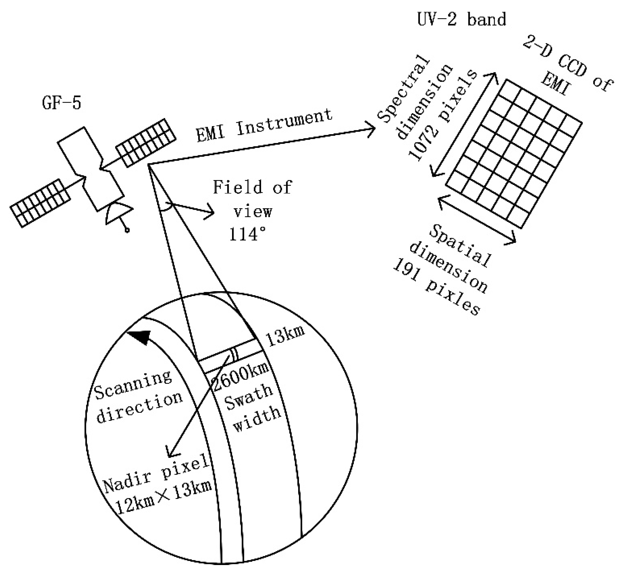
2.1. EMI Data
2.2. Auxiliary Data
2.2.1. Satellite Data
2.2.2. Ground-Based Data
3. TOC Retrieval Algorithm
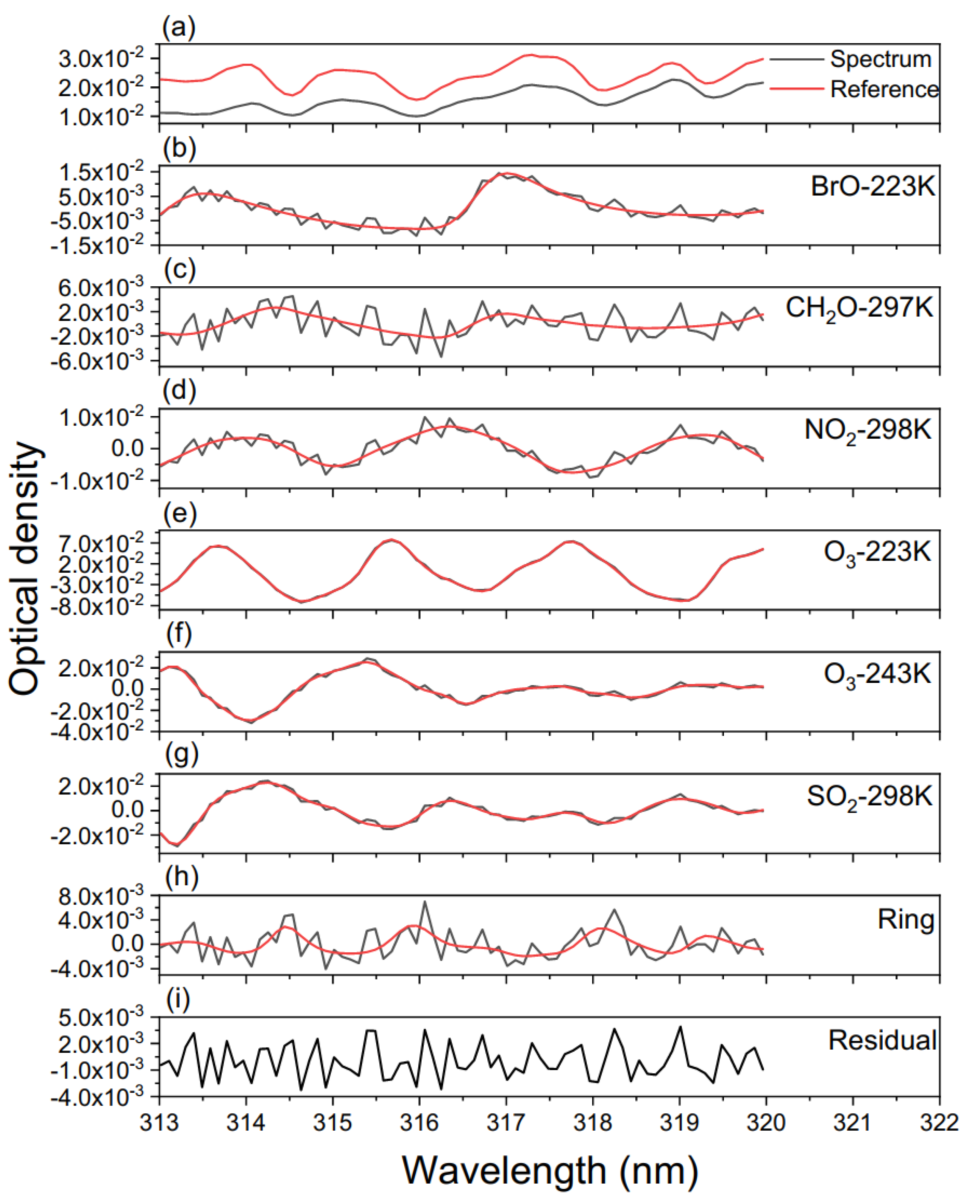
3.1. SCD Retrieval
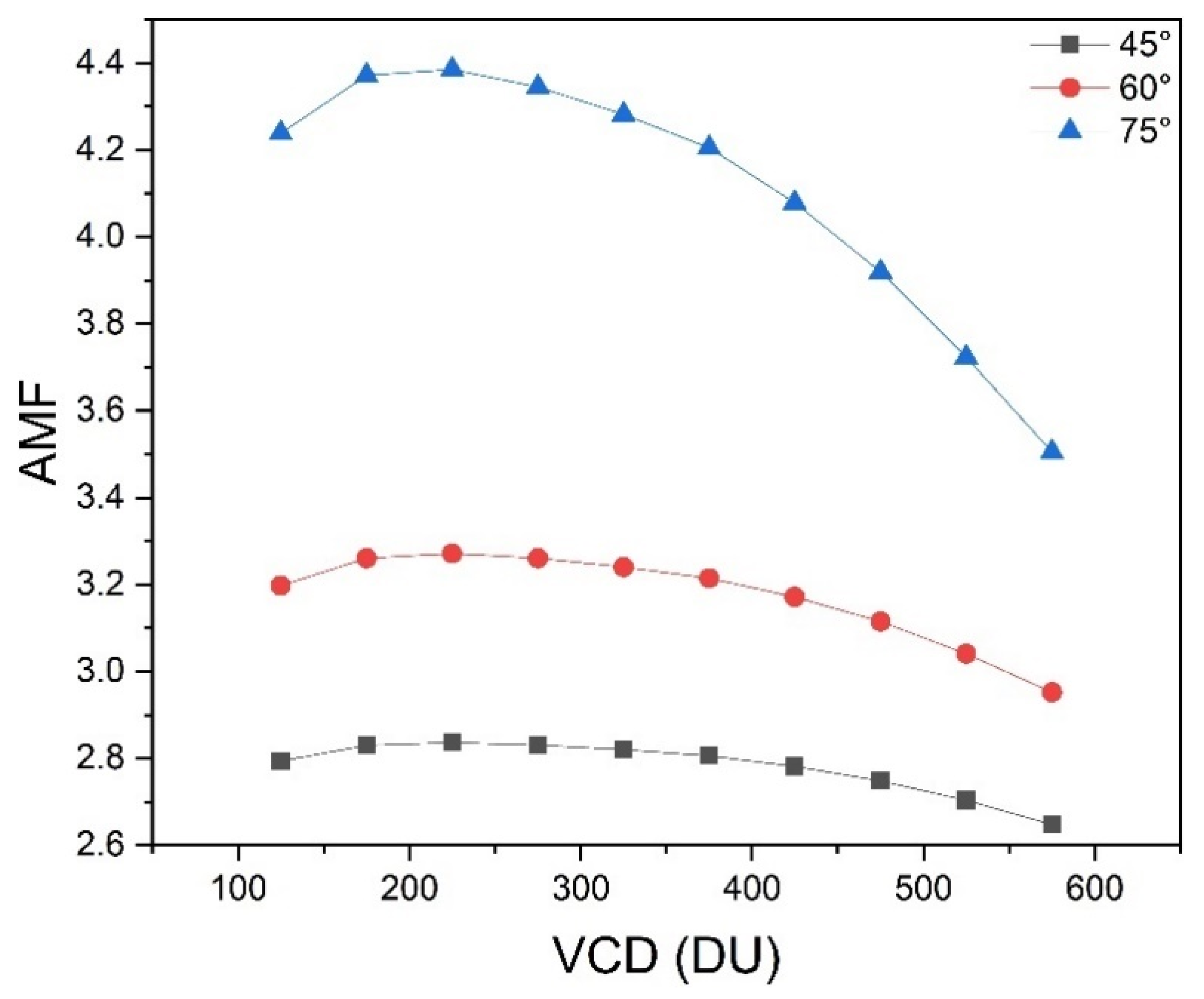
3.2. AMF Retrieval
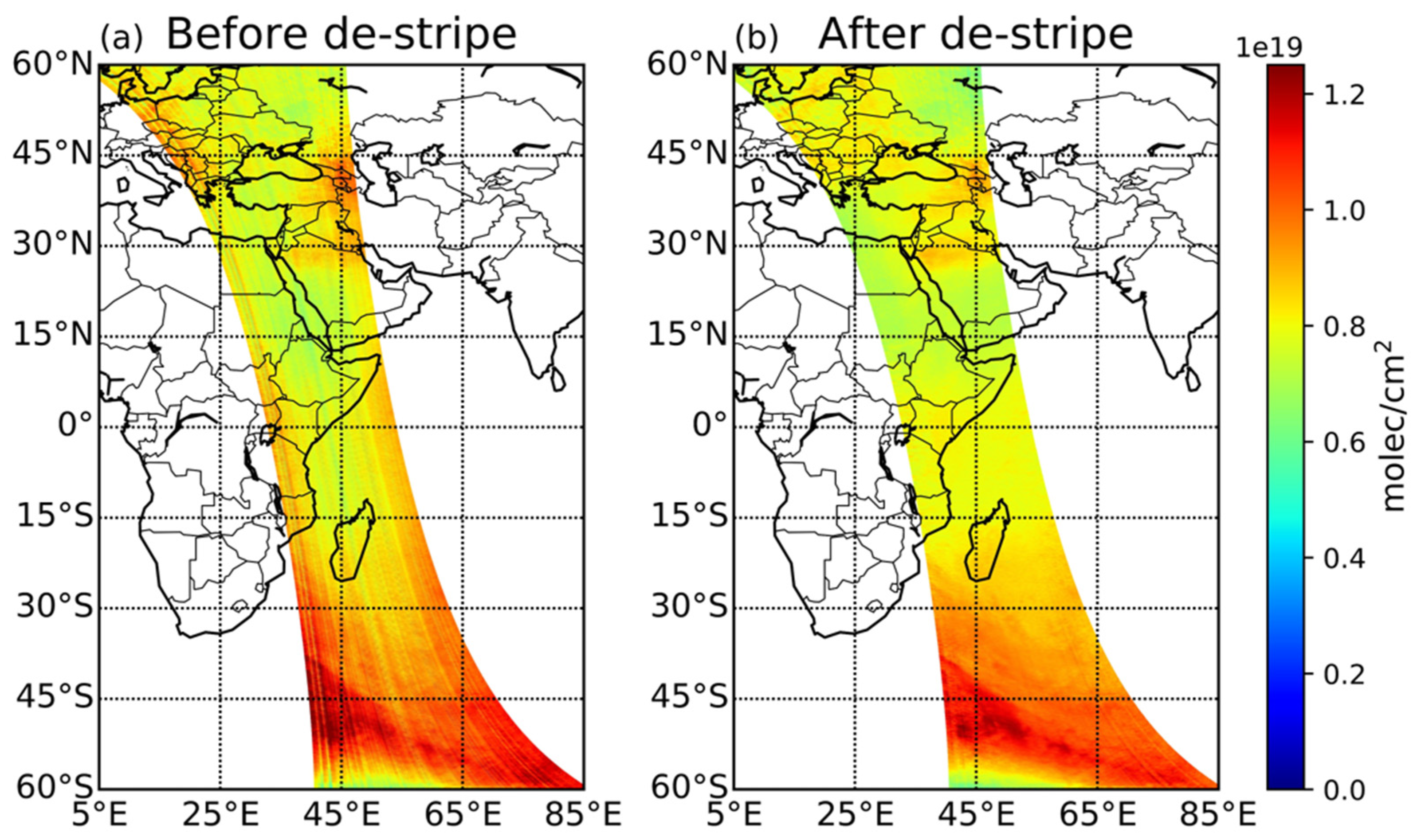
3.3. De-Stripe
- Determine the window (191 across track by 50 along track pixels) with the minimum variance of TOC.
- Calculate the average TOC in the along-track direction, giving 191 average TOC values.
- Obtain the lowest frequency term and high-frequency terms (except the lowest frequency term) using Fourier transformation from 191 averaged values. The 191 high-frequency terms are correction values, which are considered to be noise.
- Perform the stripe correction by subtracting the correction values in step 3.
3.4. Error Analysis
4. Results and Validations
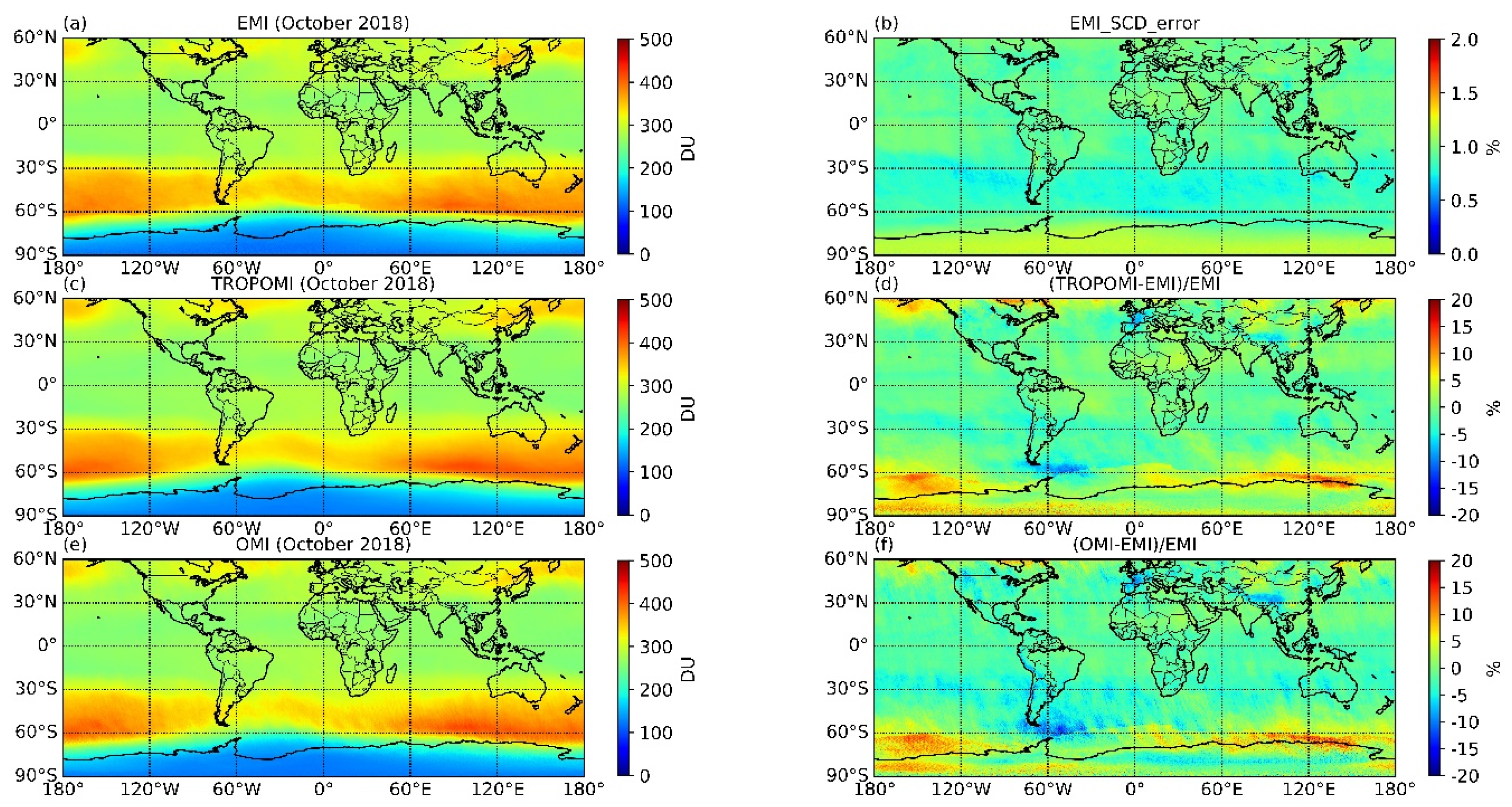
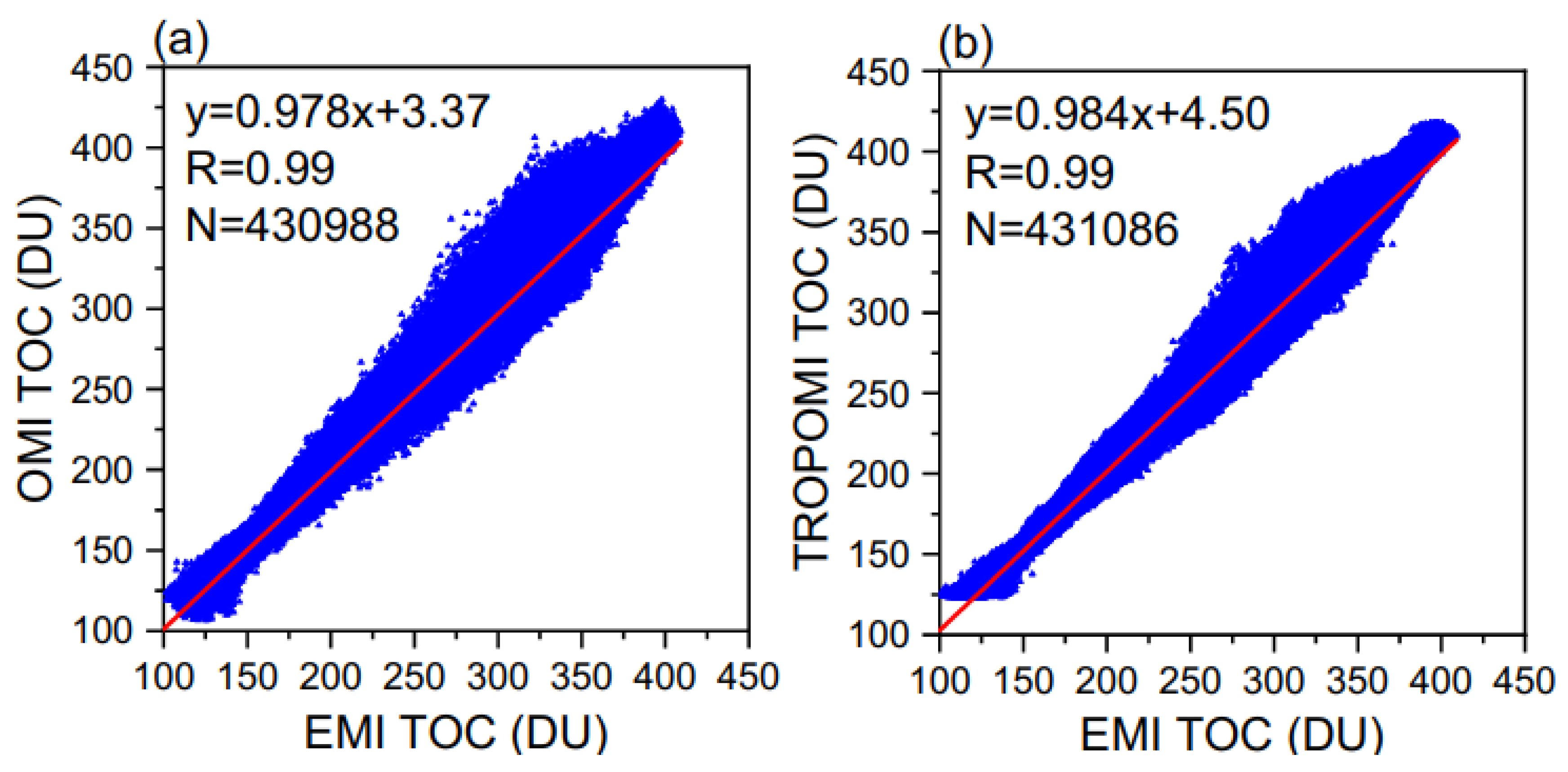
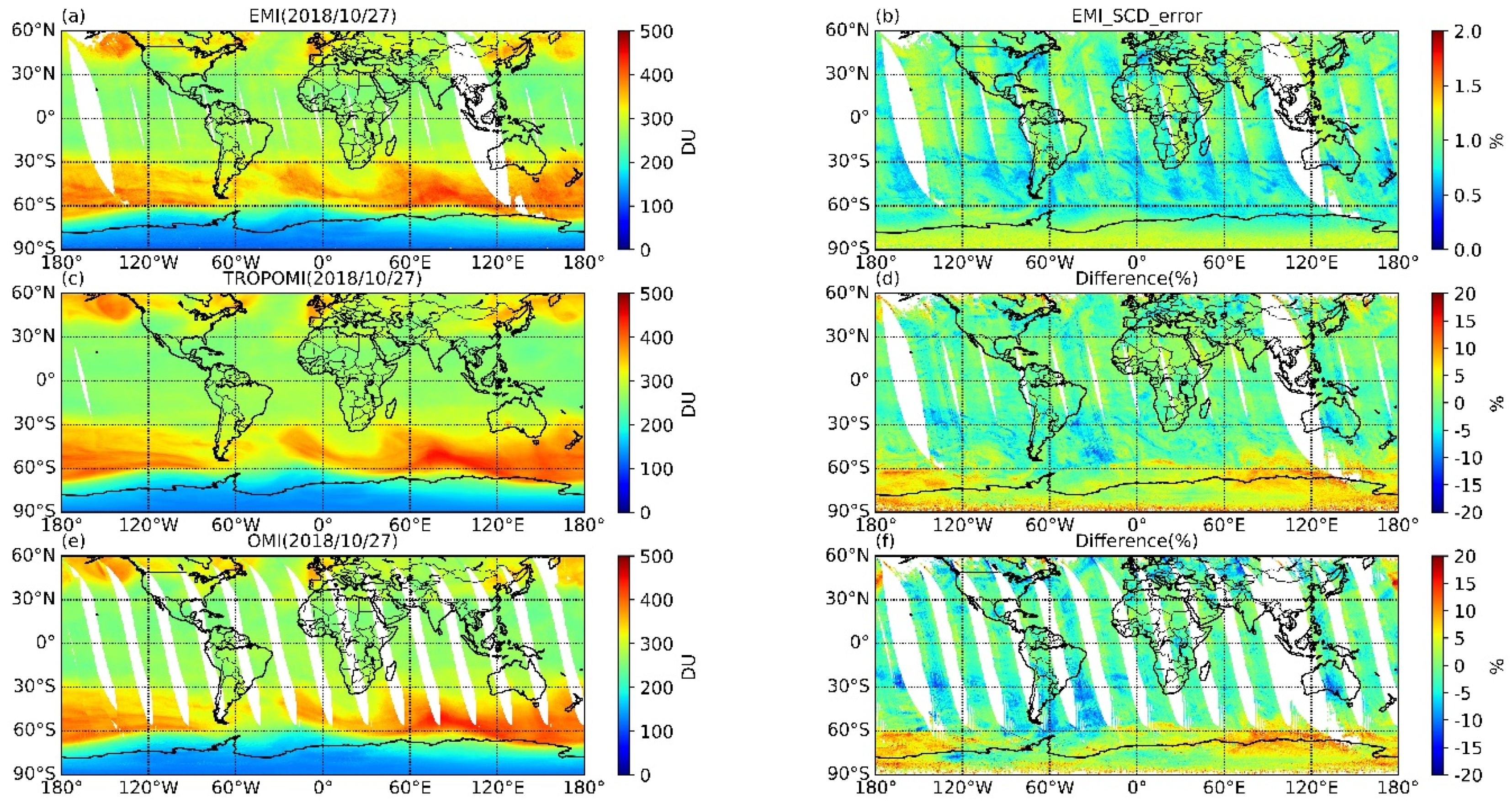
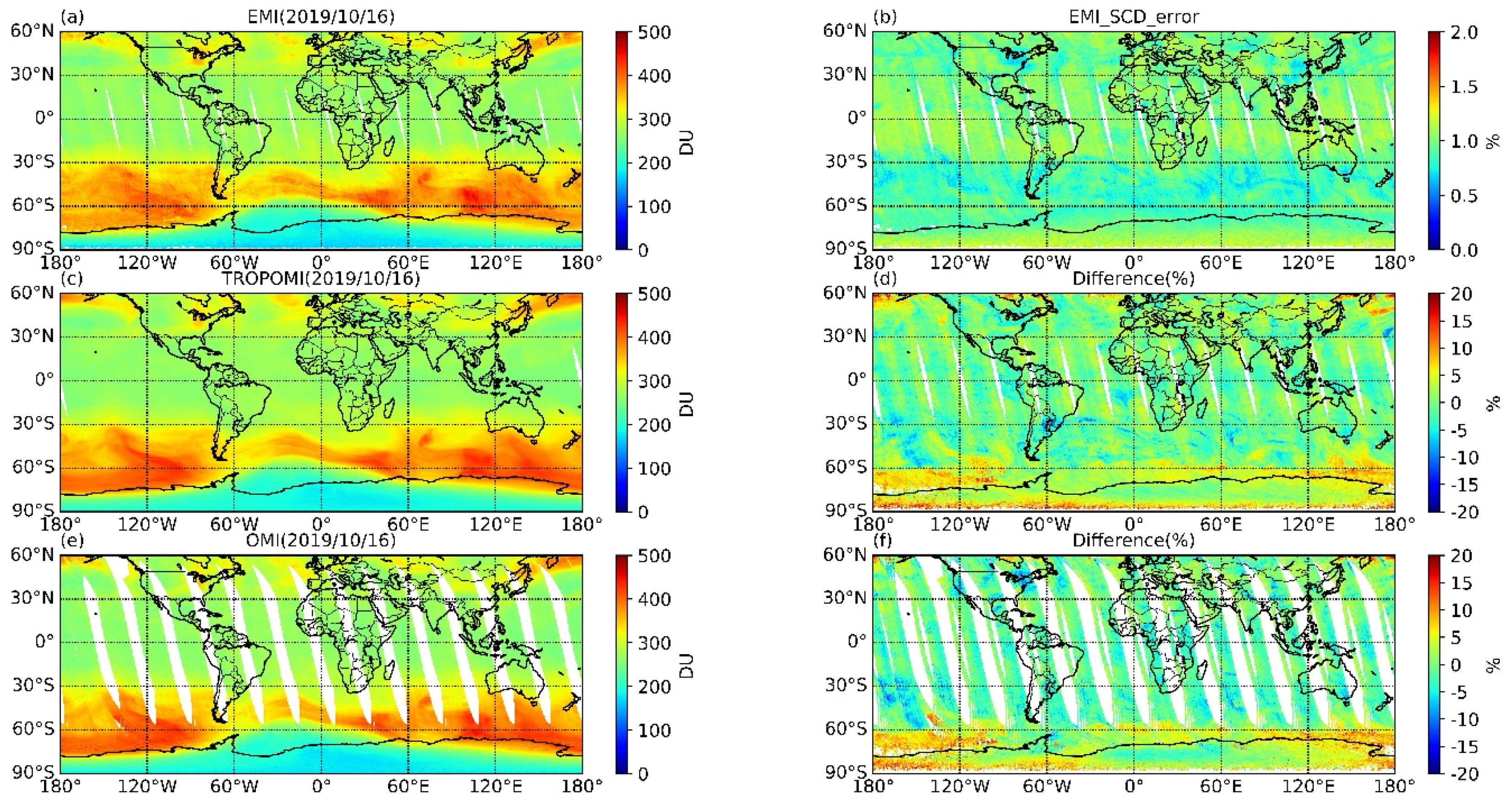
4.1. EMI Versus OMI and TROPOMI
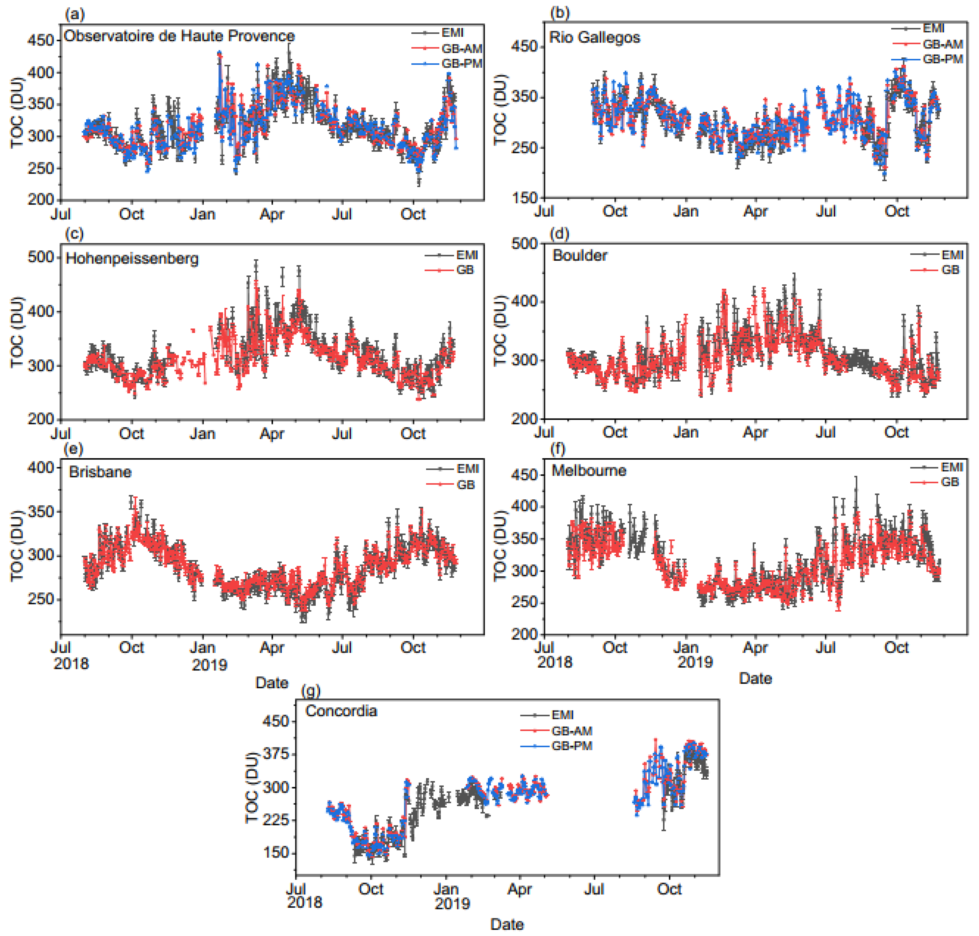
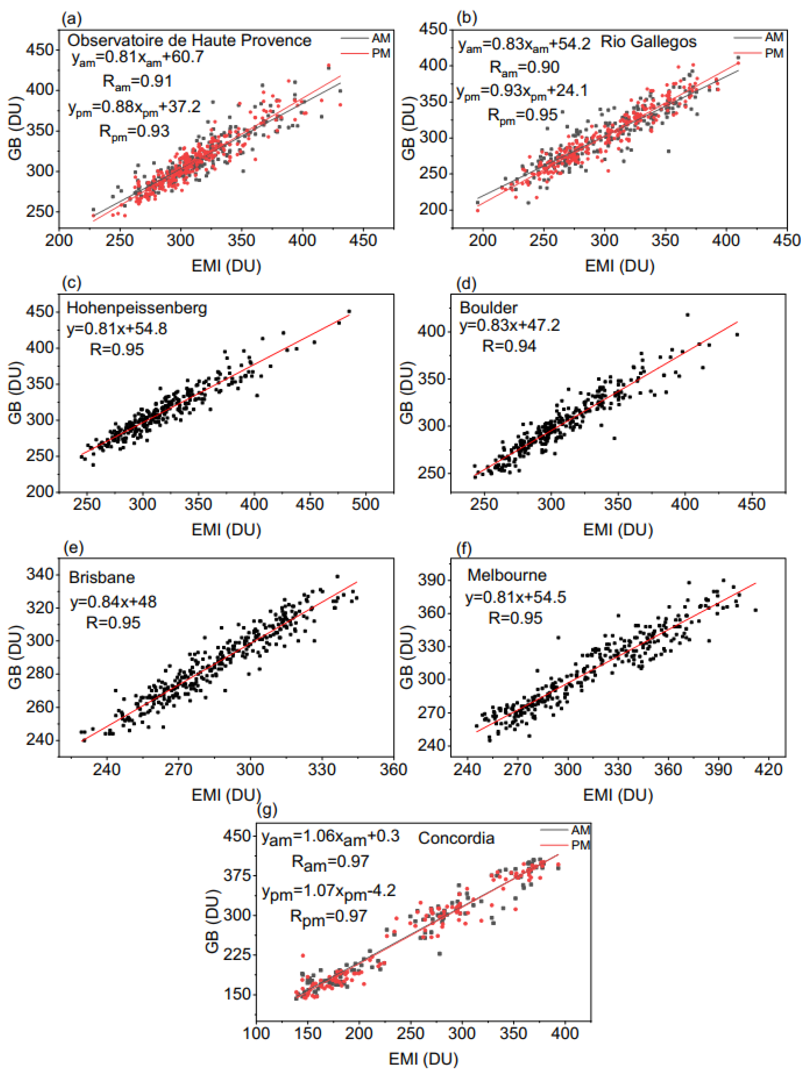
4.2. EMI Versus GB Measurements
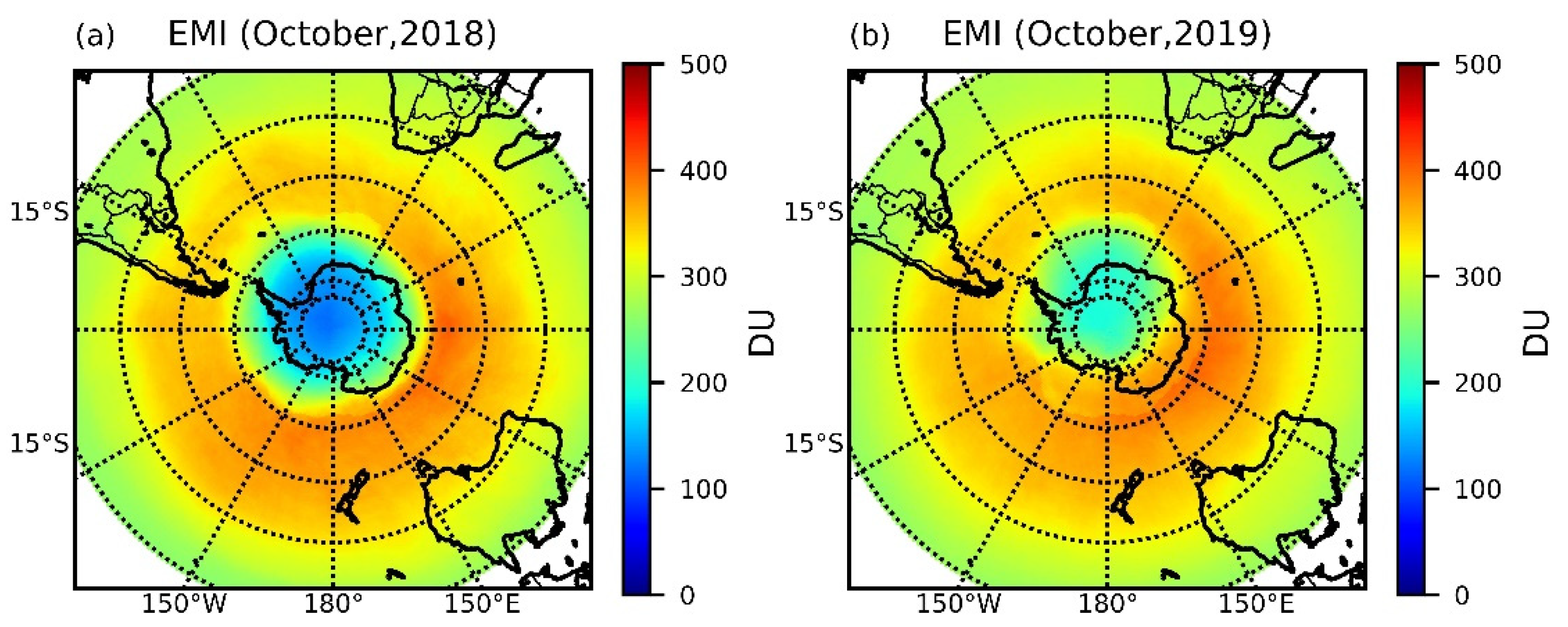
4.3. Application Case
5. Conclusions and Discussions
Author Contributions
Funding
Institutional Review Board Statement
Informed Consent Statement
Data Availability Statement
Acknowledgments
Conflicts of Interest
Appendix A


References
- Li, G.; Tan, Y.K.; Li, C.Y.; Chen, S.C.; Bai, T.; Yang, D.Y.; Zhang, Y. Characteristics of boreal winter total ozone distribution in the northern hemisphere and their relationship with stratospheric temperature during recent 30 years. Chin. J. Geophys. 2015, 58, 213–228. [Google Scholar] [CrossRef]
- Bazhenov, O. Increased humidity in the stratosphere as a possible factor of ozone destruction in the Arctic during the spring 2011 using Aura MLS observations. Int. J. Remote Sens. 2019, 40, 3448–3460. [Google Scholar] [CrossRef]
- Paschou, P.; Koukouli, M.E.; Balis, D.; Lerot, C.; Roozendael, M.V. The effect of considering polar vortex dynamics in the validation of satellite total ozone observations. Atmos. Res. 2020, 238, 104870. [Google Scholar] [CrossRef]
- Frieβ, U.; Kreher, K.; Johnston, P.V.; Platt, U. Ground-based DOAS measurements of stratospheric trace gases at two Antarctic stations during the 2002 ozone hole period. J. Atmos. Sci. 2005, 62, 765–777. [Google Scholar] [CrossRef]
- Nakajima, H.; Murata, I.; Nagahama, Y.; Akiyoshi, H.; Saeki, K.; Kinase, T.; Takeda, M.; Tomikawa, Y.; Jones, N.B. Chlorine partitioning near the polar vortex edge observed with ground-based FTIR and satellites at Syowa station, Antarctica, in 2007 and 2011. Atmos. Chem. Phys. 2020, 20, 1043–1074. [Google Scholar] [CrossRef] [Green Version]
- Farman, J.C.; Gardiner, B.G.; Shanklin, J.D. Large losses of total ozone in Antarctica reveal seasonal interaction. Nature 1985, 315, 207–210. [Google Scholar] [CrossRef]
- Solomon, S.; Lvy, D.J.; Kinnison, D.; Mills, M.J.; Neel, R.R.; Schmidt, A. Emergence of healing in the Antarctic ozone layer. Science 2016, 353, 269–274. [Google Scholar] [CrossRef] [Green Version]
- Bodeker, G.E.; Shiona, H.; Eskes, H. Indicators of Antarctic ozone depletion. Atmos. Chem. Phys. 2005, 5, 2603–2615. [Google Scholar] [CrossRef] [Green Version]
- Kerr, R.A. First detection of ozone hole recovery claimed. Science 2011, 332, 160. [Google Scholar] [CrossRef]
- Luo, Y.H.; Si, F.Q.; Liu, W.Q.; Sun, L.G.; Liu, Y. Observations of stratospheric ozone above Ny-Ålesund in the Arctic, 2010–2011. Adv. Polar Sci. 2015, 26, 256–263. [Google Scholar] [CrossRef]
- Veefkind, J.P.; de Han, J.F.; Brinksma, E.J.; Kroon, M.; Levelt, P.F. Total ozone from the ozone monitoring instrument (OMI) using the DOAS technique. IEEE Trans. Geosci. Remote Sens. 2006, 44, 1239–1244. [Google Scholar] [CrossRef]
- Loyola, D.G.; Koukouli, M.E.; Valks, P.; Bails, D.S.; Hao, N.; Van Roozendael, M.; Spurr, R.J.D.; Zimmer, W.; Kiemle, S.; Lerot, C.; et al. The GOME-2 total column ozone product: Retrieval algorithm and ground-based validation. J. Geophys. Res. 2011, 116, D07302. [Google Scholar] [CrossRef]
- Garane, K.; Koukouli, M.E.; Verhoelst, T.; Lerot, C.; Heue, K.P.; Fioletov, V.; Balis, D.; Bais, A.; Bazureau, A.; Dehn, A.; et al. TROPOMI/S5P total ozone column data: Global ground-based validation and consistency with other satellite missions. Atmos. Meas. Tech. 2019, 12, 5263–5287. [Google Scholar] [CrossRef] [Green Version]
- Burrows, J.P.; Weber, M.; Buchwitz, M.; Rozanov, V.; Ladstätter-Weißenmayer, A.; Richter, A.; Debeek, R.; Hoogen, R.; Bramstedt, K.; Eichmann, K.U.; et al. The global ozone monitoring experiment (GOME): Mission concept and first scientific results. J. Atmos. Sci. 1999, 56, 151–175. [Google Scholar] [CrossRef]
- Callies, J.; Corpaccioli, E.; Eisinger, M.; Hahne, A.; Lefebvre, A. Gome-2-Metop’s second-generation sensor for operational ozone monitoring. ESA Bull. Eur. Space 2000, 102, 28–36. [Google Scholar]
- Bovensmann, H.; Burrows, J.P.; Buchwitz, M.; Frerick, J.; Noel, S.; Rozanov, V.V.; Chance, K.V.; Goede, A.P.H. SCIAMACHY: Mission objectives and measurement modes. J. Atmos. Sci. 1999, 56, 127–150. [Google Scholar] [CrossRef] [Green Version]
- Wang, Y.M.; Wang, Y.J.; Wang, W.H.; Zhang, Z.M.; Lü, J.G.; Fu, L.P.; Jiang, F.; Chen, J.; Wang, J.H.; Guan, F.J.; et al. FY-3 satellite ultraviolet total ozone unit. Chin. Sci. Bull. 2009, 55, 84–89. [Google Scholar] [CrossRef]
- Levelt, P.F.; Joiner, J.; Tamminen, J.; Veefkind, J.P.; Bhartia, P.K.; Stein Zweers, D.C.; Duncan, B.N.; Streets, D.G.; Eskes, H.; van der A, R.; et al. The ozone monitoring instrument: Overview of 14 years in space. Atmos. Chem. Phys. 2018, 18, 5699–5745. [Google Scholar] [CrossRef] [Green Version]
- Veefkind, J.P.; Aben, I.; McMullan, K.; Förster, H.; de Vries, J.; Otter, G.; Claas, J.; Eskes, H.J.; de Haan, J.F.; Kleipool, Q.; et al. TROPOMI on the ESA sentinel-5 precursor: A GMES mission for global observations of the atmospheric composition for climate, air quality and ozone layer applications. Remote Sens. Environ. 2012, 120, 70–83. [Google Scholar] [CrossRef]
- Platt, U.; Stutz, J. Differential Optical Absorption Spectroscopy: Principles and Applications; Springer: Berlin/Heidelberg, Germany, 2008. [Google Scholar]
- Buchard, V.; Brogniez, C.; Auriol, F.; Bonnel, B.; Lenoble, J.; Tanskanen, A.; Bojkov, B.; Veefkind, P. Comparison of OMI ozone and UV irradiance data with ground-based measurements at two French sites. Atmos. Chem. Phys. 2008, 8, 4517–4528. [Google Scholar] [CrossRef] [Green Version]
- Cheng, L.X.; Tao, J.H.; Valks, P.; Yu, C.; Liu, S.; Wang, Y.P.; Xiong, X.Z.; Wang, Z.F.; Chen, L.F. NO2 retrieval from the environmental trace gases monitoring instrument (EMI): Preliminary results and intercomparison with OMI and TROPOMI. Remote Sens. 2019, 11, 3017. [Google Scholar] [CrossRef] [Green Version]
- Zhang, C.X.; Liu, C.; Chan, K.L.; Hu, Q.H.; Liu, H.R.; Li, B.; Xing, C.Z.; Tan, W.; Zhou, H.J.; Si, F.Q.; et al. First observation of tropospheric nitrogen dioxide from the environmental trace gases monitoring instrument onboard the Gaofen-5 satellite. Light Sci. Appl. 2020, 9, 66. [Google Scholar] [CrossRef] [PubMed] [Green Version]
- Zhao, M.J.; Si, F.Q.; Zhou, H.J.; Wang, S.M.; Jiang, Y.; Liu, W.Q. Preflight calibration of the Chinese environmental trace gases monitoring instrument (EMI). Atmos. Meas. Tech. 2018, 11, 5403–5419. [Google Scholar] [CrossRef] [Green Version]
- Thomas, H.E.; Watson, I.M.; Simon, A.C.; Prata, A.J.; Realmuto, V.J. A comparison of AIRS, MODIS and OMI sulphur dioxide retrievals in volcanic clouds. Geomat. Nat. Haz. Risk. 2011, 2, 217–232. [Google Scholar] [CrossRef]
- Inness, A.; Flemming, J.; Heue, K.P.; Lerot, C.; Loyola, D.; Ribas, R.; Valks, P.; van Roozendael, M.; Xu, J.; Zimmer, W. Monitoring and assimilation tests with TROPOMI data in the CAMS system: Near-real-time total column ozone. Atmos. Chem. Phys. 2019, 19, 3939–3962. [Google Scholar] [CrossRef] [Green Version]
- Smedley, A.R.D.; Rimmer, J.S.; Webb, A.R. A more representative “best representative value” for daily total column ozone reporting. Atmos. Meas. Tech. 2017, 10, 4697–4704. [Google Scholar] [CrossRef] [Green Version]
- Bogumil, K.; Orphal, J.; Homann, T.; Voigt, S.; Spietz, P.; Fleischmann, O.C.; Vogel, A.; Hartmann, M.; Kromming, H.; Bovensman, H.; et al. Measurements of molecular absorption spectra with the SCIAMACHY preflight model: Instrument characterization and reference data for atmospheric remote-sensing in the 230–2380 nm region. J. Photochem. Photobiol. A Chem. 2003, 157, 167–184. [Google Scholar] [CrossRef]
- Vandaele, A.C.; Hermans, C.; Simon, P.C.; Roozendael, M.V.; Guilmot, J.M.; Carleer, M.; Colin, R. Fourier transform measurement of NO2 absorption cross-section in the visible range at room temperature. J. Atmos. Chem. 1996, 25, 289–305. [Google Scholar] [CrossRef] [Green Version]
- Vandaele, A.C.; Hermans, C.; Fally, S. Fourier transform measurements of SO2 absorption cross sections: II.: Temperature dependence in the 29000-44000 cm−1 (227–345 nm) region. J. Quant. Spectrosc. Ra. 2009, 110, 2115–2126. [Google Scholar] [CrossRef]
- Fleischmann, O.C.; Hartmann, M. New ultraviolet absorption cross-sections of BrO at atmospheric temperatures measured by time-windowing Fourier transform spectroscopy. J. Photochem. Photobiol. 2004, 168, 117–132. [Google Scholar] [CrossRef]
- Meller, R.; Moortgat, G.K. Temperature dependence of the absorption cross sections of formaldehyde between 223 and 323 K in the wavelength range 225–375 nm. J. Geophys. Res. 2000, 105, 7089–7101. [Google Scholar] [CrossRef]
- Wellemeyer, C.G.; Bhartia, P.K.; Taylor, S.L.; Qin, W.; Ahn, C. Version 8 total ozone mapping spectrometer (TOMS) algorithm. Quadrenn. Ozone Symp. 2004, I, 635–636. [Google Scholar]
- Kleipool, Q.L.; Dobber, M.R.; de Haan, J.F.; Levelt, P.E. Earth surface reflectance climatology from 3 years of OMI data. J. Geophys Res. Atmos. 2008, 113. [Google Scholar] [CrossRef]
- Boersma, K.F.; Eskes, H.J.; Veefkind, J.P.; Brinksma, E.J.; Sneep, M.V.; Van den Oord, G.H.; Levelt, P.F.; Stammes, P.; Gleason, J.F.; Bucsela, E.J. Near-real time retrieval of tropospheric NO2 from OMI. Atmos. Chem. Phys. 2007, 7, 2103–2118. [Google Scholar] [CrossRef] [Green Version]
- Qian, Y.Y.; Luo, Y.H.; Si, F.Q.; Yang, T.P.; Yang, D.S. Three-year observations of ozone columns over polar vortex edge area above West Antarctica. Adv. Atmos. Sci. 2021. [Google Scholar] [CrossRef]
- Bodeker, G.E.; Struthers, H.; Connor, B.J. Dynamical containment of Antarctic ozone depletion. Geophys. Res. Lett. 2002, 29, 2-1–2-4. [Google Scholar] [CrossRef]
- Safieddine, S.; Bouillon, M.; Paracho, A.C.; Jumelet, J.; Tence, F.; Pazmino, A.; Goutail, F.; Wespes, C.; Bekki, S.; Boynard, A.; et al. Antarctic ozone enhancement during the 2019 sudden stratospheric warming event. Geophys. Res. Lett. 2020, 47, e2020GL087810. [Google Scholar] [CrossRef]


| Parameter | EMI | OMI | TROPOMI |
|---|---|---|---|
| Detection wavelength | 240–710 nm | 270–500 nm | 270–550, 675–775, and 230–2385 nm |
| Spectral resolution | 0.3–0.5 nm | 0.5 nm | 0.225–0.65 nm |
| Spatial resolution (nadir) | 12 × 13 km2 | 13 × 24 km2 | 3.5 × 5.5 km2 |
| Field of view | 114° | 114° | 108° |
| Flight height | 705 km | 705 km | 824 km |
| Fitting window for TOC product | 313–320 nm | 331.1–336.1 nm | 325–335 nm |
| Radiative transfer model for AMF calculation | SCIATRAN | Doubling-Adding-KNMI (DAK) | Vector Linearized Discrete Ordinate Radiative Transfer (VLIDORT) |
| Parameter | Settings |
|---|---|
| Fitting Interval | 313–320 nm |
| Polynomial | Order 4 |
| Cross-sections | |
| O3 | 223 K, 243 K, [28] |
| NO2 | 298 K, [29] |
| SO2 | 298 K, [30] |
| BrO | 223 K, [31] |
| HCHO | 297 K, [32] |
| Ring | Calculated using QDOAS |
| Parameter | Number of Nodes | Values |
|---|---|---|
| SZA (°) | 18 | 0, 10, 20, 30, 35, 40, 45, 50, 55, 60, 65, 70, 72, 74, 76, 78, 80, 82 |
| RAA (°) | 5 | 0, 45, 90, 135, 180 |
| VZA (°) | 13 | 0, 5, 10, 15, 20, 25, 30, 35, 40, 45, 50, 55, 60 |
| Latitude (°) | 18 | −85, −75, −65, −55, −45, −35, −25, −15, −5, 5, 15, 25, 35, 45, 55, 65, 75, 85 |
| Albedo | 9 | 0, 0.05, 0.1, 0.20, 0.30, 0.40, 0.60, 0.80, 1.0 |
| Cloud pressure (hPa) | 9 | 1013, 795, 701, 616, 472, 356, 264, 164, 96 |
| Month | 12 | 1, 2, 3, 4, 5, 6, 7, 8, 9, 10, 11, 12 |
| VCD (DU) for AMF correction | 10 | 125, 175, 225, 275, 325, 375, 425, 475, 525, 575 |
| Error Sources | Relative Error (%) |
|---|---|
| Aerosols | 0.8 |
| Albedo | 0.3 |
| Cloud pressure | <1.5 |
| Cloud fraction | <0.5 |
| SCD | <2 |
| Ozone profiles | <3.0 (SZA < 80°) |
| <3.6 (SZA < 82°) |
| Station | Latitude, Longitude | Method | Averaged Difference (95% Confidence Interval) | Number of Measurement Days | Root Mean Square Relative Error (RMSRE) |
|---|---|---|---|---|---|
| Hohenpeissenberg, Germany | 47.80° N, 11.02° E | Brewer | 3.30% | 281 | 4.4% |
| Observatoire de Haute Provence, France | 43.94° N, 5.71° E | SAOZ | 3.02% | 284 | 4.1% |
| Boulder, CO, United States | 39.99° N, 105.26° W | Dobson | 2.97% | 300 | 4.0% |
| Brisbane, Australia | 27.39° S, 153.13° E | Dobson | 2.10% | 329 | 2.8% |
| Melbourne, Australia | 37.81° S, 144.97° E | Dobson | 3.34% | 299 | 4.3% |
| Rio Gallegos, Argentina | 51.60° S, 69.32° W | SAOZ | 4.13% | 247 | 5.3% |
| Concordia Dome C, Antarctica | 75.10° S, 123.35° E | SAOZ | 5.47% | 129 | 9.0% |
Publisher’s Note: MDPI stays neutral with regard to jurisdictional claims in published maps and institutional affiliations. |
© 2021 by the authors. Licensee MDPI, Basel, Switzerland. This article is an open access article distributed under the terms and conditions of the Creative Commons Attribution (CC BY) license (https://creativecommons.org/licenses/by/4.0/).
Share and Cite
Qian, Y.; Luo, Y.; Si, F.; Zhou, H.; Yang, T.; Yang, D.; Xi, L. Total Ozone Columns from the Environmental Trace Gases Monitoring Instrument (EMI) Using the DOAS Method. Remote Sens. 2021, 13, 2098. https://0-doi-org.brum.beds.ac.uk/10.3390/rs13112098
Qian Y, Luo Y, Si F, Zhou H, Yang T, Yang D, Xi L. Total Ozone Columns from the Environmental Trace Gases Monitoring Instrument (EMI) Using the DOAS Method. Remote Sensing. 2021; 13(11):2098. https://0-doi-org.brum.beds.ac.uk/10.3390/rs13112098
Chicago/Turabian StyleQian, Yuanyuan, Yuhan Luo, Fuqi Si, Haijin Zhou, Taiping Yang, Dongshang Yang, and Liang Xi. 2021. "Total Ozone Columns from the Environmental Trace Gases Monitoring Instrument (EMI) Using the DOAS Method" Remote Sensing 13, no. 11: 2098. https://0-doi-org.brum.beds.ac.uk/10.3390/rs13112098