Article

3D Mesh Pre-Processing Method Based on Feature Point Classification and Anisotropic Vertex Denoising Considering Scene Structure Characteristics

1
Key Laboratory of Urban Land Resources Monitoring and Simulation, Ministry of Natural Resources, Shenzhen 518034, China
2
State Key Laboratory of Information Engineering in Surveying, Mapping and Remote Sensing, Wuhan University, Wuhan 430072, China
*
Author to whom correspondence should be addressed.
Current address: No.129 Luoyu Road, Hongshan District, Wuhan 430079, China.
These authors contributed equally to this work.
Remote Sens. 2021, 13(11), 2145; https://0-doi-org.brum.beds.ac.uk/10.3390/rs13112145
Submission received: 17 April 2021 / Revised: 13 May 2021 / Accepted: 21 May 2021 / Published: 29 May 2021
(This article belongs to the Special Issue 3D Modelling from Point Cloud: Algorithms and Methods)

Abstract

:
3D mesh denoising plays an important role in 3D model pre-processing and repair. A fundamental challenge in the mesh denoising process is to accurately extract features from the noise and to preserve and restore the scene structure features of the model. In this paper, we propose a novel feature-preserving mesh denoising method, which was based on robust guidance normal estimation, accurate feature point extraction and an anisotropic vertex denoising strategy. The methodology of the proposed approach is as follows: (1) The dual weight function that takes into account the angle characteristics is used to estimate the guidance normals of the surface, which improved the reliability of the joint bilateral filtering algorithm and avoids losing the corner structures; (2) The filtered facet normal is used to classify the feature points based on the normal voting tensor (NVT) method, which raised the accuracy and integrity of feature classification for the noisy model; (3) The anisotropic vertex update strategy is used in triangular mesh denoising: updating the non-feature points with isotropic neighborhood normals, which effectively suppressed the sharp edges from being smoothed; updating the feature points based on local geometric constraints, which preserved and restored the features while avoided sharp pseudo features. The detailed quantitative and qualitative analyses conducted on synthetic and real data show that our method can remove the noise of various mesh models and retain or restore the edge and corner features of the model without generating pseudo features.

1. Introduction

The 3D mesh model is widely used in 3D space measurement and positioning technology, augmented reality (AR) and virtual reality (VR), auxiliary medical analysis, industrial measurement, cultural heritage protection or restoration, etc. [1]. However, due to the influence of the measurement environment, the limitation of data acquisition accuracy, the 3D mesh data inevitably has different degrees of noise, which seriously affects the surface accuracy of reconstruction. This poses a huge obstacle to the practical application of the 3D mesh model, and it must be preprocessed by appropriate mesh denoising methods. Therefore, we directly focus on the accuracy and integrity of feature recognition and feature recovery in the process of denoising in this paper.
3D mesh denoising seeks to eliminate the noise on the surface, which has recently become a major focus of 3D mesh pre-processing method research. The challenging nature of mesh denoising is recovering the structural features of the surface without introducing false features into the smooth area when evolving a noisy mesh to its unknown noise-free counterpart [2]. Many mesh denoising attempts directly filter vertex positions [3] or facet normals followed by updating vertex positions [4]. However, vertex positions and surface normals are both sensitive to noise, and they even become unreliable when the noise level increases in denoising [2]. Recently, the GMNF method [5] was proposed to overcome the noise sensitivity of facet normals. Nevertheless, it loses corners during the denoising process, since the estimation of the guiding normals did not take sufficient account of the vicinity of corners. Moreover, a local patch employed for normal estimation will exhibit artifact pseudofeatures. These denoising methods make the indiscriminate application of filtering and denoising, which makes structural features oversmoothed or produce artifacts in the flat transition area in denoising results. More recently, with the development of learning-based methodology, data-driven methods have been used in 3D mesh model denoising [6], which do not need manual input to extract features. However, these methods require paired data (noisy meshes with ground truths) for training, and the reliability heavily depends on the initial training data set.
Feature points are an important representation of the geometric structure attributes of 3D models; they constitute the contour features of 3D models and highlight the boundary and geometric structure of 3D scenes, which are the key basis for retaining and restoring structural features in the process of 3D model mesh denoising. To better retain sharp features, researchers began to explore feature-based denoising methods [7,8,9], they first classify feature vertices and then apply different denoising strategies to update the vertex position. However, due to the noise sensitivity of surface normals, the detected features may suffer from information loss or confusion.
To address these issues, we propose building a fully automated pipeline that removes the noise on the surface of a 3D model while preserving its structural features. Our pipeline consists of three major modules, namely normal filtering, feature point classification and vertex denoising. Our method first uses the guidance normal that considers the angle characteristics to carry out joint bilateral filtering and filter the surface normal. Subsequently, to accurately classify the non-feature points, feature edge points and feature corner points, we adopt filtered face normals to calculate the normal vote tensor matrix of vertices and use its eigenvalues to classify the vertices. Then, we apply an isotropic neighborhood to update the non-feature points to denoise the non-characteristic regions and to take into account the geometric corrugation lines. Finally, we utilize the local support plane constraint of the feature points and the dihedral angle constraint of the local sharp edges to denoise the feature region. Our method enables 3D mesh models to obtain and restore geometric features and avoid producing sharp false features when denoising. The experimental results on different data types, including CAD data, 3D scan data and 3D mesh data reconstructed from oblique images show that our method achieves significant and consistent improvement compared to all baseline methods by considering scene structure characteristics. We summarize the contributions of the proposed method as follows:
(1) A facet normal filtering method considering corner features is proposed, which improves the robustness of the filtering algorithm by improving the guided mesh normal filtering (GMNF) method. The experiments show that the proposed method can accurately recover corner features.
(2) An accurate classification method for noise points was proposed based on the normal voting tensor (NVT) of the vertex using filtered facet normals from noise models. It can accurately classify the feature points and non-feature points in the model to avoid preprocessing the model and reduce the loss of detailed features when classifying noisy vertices.
(3) An anisotropic stepwise vertex denoising method is proposed. Compared with the traditional method, different strategies are used to design the vertex update strategy in the non-feature area and the feature area, and the vertex position is updated step by step. The local dihedral angle constraint is used to avoid smoothing and increase the sharpening of the local sharp edges during the denoising iterations. Therefore, the denoised model maintains structural characteristics and reduces pseudofeatures as much as possible.

2. Literature Review

In this section, we briefly review the related work on 3D mesh denoising. We present the isotropic and anisotropic 3D model denoising methods without going into detail, aiming to summarize the current classic and commonly used methods.

2.1. Isotropic Mesh Filtering

Isotropic filtering methods do not consider the surface features or the directions of the features, which will cause the model to shrink, blur or lose characteristics when filtering noise. The early Laplacian-based method [10,11] is simple and efficient; the Laplacian denoising method recursively moves each vertex of the mesh by a displacement equal to a positive scale factor times the average of the neighboring vertices. However, there is an inevitable mesh shrinkage problem. Taubin [12] sampled a surface signal low-pass filter algorithm, which can remove noise while preserving the volume to a certain extent, reducing model shrinkage. The mean curvature flow [13] is used to process irregular surfaces, and the method combining Laplace smooth flow and discrete mean curvature flow [14] aims to reduce oversmoothing. Spectral methods for mesh processing and analysis [15] use eigenvalues, eigenvectors, or eigenspace projections to separate 3D mesh data from noise. The main disadvantage of these isotropic methods is the lack of consideration of the geometric characteristics of the model; the characteristics of the model will be blurred or lost when filtering noise. In our work, we designed an anisotropic denoising scheme to better maintain the characteristics of the models.

2.2. Anisotropic Mesh Filtering

Since the method of isotropic model denoising did not consider the characteristics of the model very well, later researchers studied many anisotropic denoising methods, which considered the characteristics of the model, and the focus was on how to preserve the model while denoising the geometric features.
Optimization-based methods. This kind of method formulates denoising as a vertex optimization problem and seeks a denoised mesh that can best fit the input mesh and a set of geometric priors of the ground-truth geometry [16]. However, these methods rely on the geometric priors of the noise distribution. Liu et al. [17] proposed a noniterative global optimization operator, which can maintain the characteristics of the original mesh without shrinkage or deformation. Based on the sparsity optimization ideas that have prevailed in image processing in recent years, X. Wu et al. [18] presented a variational algorithm for feature-preserving mesh denoising. However, it produces a severe staircase effect, especially for real meshes. The methods of [18,19] introduce step effects or prominent features in flat areas; the method of Liu et al. [20] avoids this problem but smooths out sharp features when the noise level increases. Zhong et al. [21] presented a normal filtering model with three sparsity terms that can restore finer features. We differ in our approach as we consider the problem of denoising as feature classification and preservation.
Regularization-based methods. Regularizers are usually used to address ill-posed problems. 3D mesh model denoising is an ill-posed problem in many cases due to sensing limitations and non-uniform sampling operations. Ohtake et al. [22] combined Laplacian flow with a function of the mean curvature to increase mesh regularity and reduce oversmoothing, but operations that do not distinguish between all vertices will lose features. The L0 [23] algorithm introduces a discrete differential edge operator and uses L0 minimization to remove noise. Wang et al. [24] presented an approach for decoupling noise and features on 3D shapes, using the proposed analysis compressed sensing optimization algorithm to progressively decompose features and noise. In our work, we classified feature vertices based on normal voting tensor using filtered normal.
Filter-based denoising methods. This is currently a very common denoising method. The bilateral filter method considers the spatial distance information and the similarity of the normals to achieve the purpose of feature preservation and denoising. A bilateral filter was first used for image filtering [25,26] owing to the edge-preserving property of the bilateral filter, and it was later applied to 3D model denoising. The BM method [3] uses a bilateral filter to directly calculate the distance that the vertex moves along its normal and iteratively filters the noise gradually. The filtering speed is fast, but it easily loses sharp structural features. The NoIter method [27] uses a bilateral filter to directly calculate the coordinates of the vertices. Since the normal of the surface can express the local surface orientation and the geometric characteristics to a large extent, many methods based on filtering normals have been proposed. They are usually divided into two steps: filtering the normal based on a bilateral filter and then updating the vertex position [4,5,28,29,30]. The principle of the GMNF method [5] is to use the consistency function to find the patch with the most consistent normal in the neighboring triangles of the face of interest and obtain the average unit normal of this patch as guidance for the face of interest. However, it may introduce pseudofeatures, and its robustness to the retention and restoration of corner features is not strong. To address this problem, Li et al. [31] improved the method: they proposed a corner-aware neighborhood (CAN) scheme, using vertex-based CANs, face-based CANs and edge-based CANs to select the patch of the face of interest, but this method makes it more complicated to choose a patch. We differ in our approach as we estimate the guide normal using the dual weight function. The RoFi method [32] filters normals by bilateral filtering and uses Tukey’s biweight function as a similarity function in bilateral weighting, which is a robust estimator that stops diffusion at sharp edges to retain features and effectively removes noise from flat regions. These filtering-based methods can preserve most of the clear features. However, due to the insufficient consideration of structural features, it may produce false features. The authors in [33] proposed a highly efficient approach for feature-preserving mesh denoising by a locally fast algorithm for initial vertex filtering and an unstandardized bilateral filter. Our goal is different since we focus on feature classification and preservation more effectively. The authors in [34] introduced a two-stage scheme to construct adaptive consistent neighborhoods for guided normal filtering. The authors in [2] proposed further choosing a more consistent sub-patch to estimate the guidance normal. The authors in [35] developed a novel patch normal co-filtering method from the nonlocal similarity prior, the guidance normal obtained from the low-rank matrix recovery. We differ in our approach as we consider corner features when estimating the guidance normals and apply an anisotropic stepwise vertex denoising method.
Learning-based methods. Sometimes also called data-driven methods, deep neural networks are usually used to process 3D (irregular) models. Wang et al. [16] suggested a data-driven method for mesh denoising with cascaded nonlinear regression functions. Similarly, Wang et al. [36] proposed a novel two-step data-driven mesh denoising approach. Zhao et al. [37] designed a deep convolutional neural network (CNN) to replace guidance normal generation and guidance filtering in GMNF [5]. Arvanitis et al. [38] extended this method to 3D meshes, making the transition from face normals to pixels, and applied it in 3D mesh denoising, but it may be sensitive to different noise patterns. X. Li et al. [6] presented a deep normal filtering network (DNF-Net) for mesh denoising, which does not need manual input to extract features. The authors in [39] proposed the use of a fully end-to-end learning strategy based on graph convolutions, which investigated the ability to learn directly from the normal information. When only using normal data, its robustness remains to be tested. However, the main limitation is that the reconstruction accuracy of important details heavily depends on whether they were initially included in the training set. It is difficult to consistently apply noisy models generated by different levels of noise and different sampling devices.
Feature-based methods. Common methods for feature recognition or the extraction of meshes represented by vertices, edges and faces include curvature-based methods [40,41], methods based on topological connections or geometric features [2], learning-based methods [42] and methods based on normal tensor voting [43,44]. The method based on the NVT easily classifies edge feature points and corner feature points, and it has been widely used in mesh denoising technology. However, this method is more sensitive to noise, which makes it very unreliable for the feature classification of noisy models. To solve this problem, the ENVT method [45] calculates the voting tensor, uses the binary optimization quantum element method (QEM) of eigenvalues to classify the feature points, uses the voting tensor feature vector to filter the surface normals anisotropically, and finally updates the vertices to adapt to the filtered face normals. The CPD method [9] is improved on the basis of the ENVT method [45]. Because vertex normals are very sensitive to noise, it is challenging to deal with noisy models. Wei et al. [7,8] first used the multiscale normal tensor voting method to classify the feature vertices and used the segmented MLS method to update the vertex position. Similarly, [46] first smooths the vertices and then classifies the feature points. These feature classification methods based on the NVT can obtain more accurate feature points after the initial denoising. Unfortunately, some details of the mesh model may be lost after the initial denoising, resulting in the incomplete preservation of the final model features. This classification scheme has difficulty identifying structural features from noise, and its reliability decreases with increasing model noise intensity.

2.3. Conclusions of the Literature Review
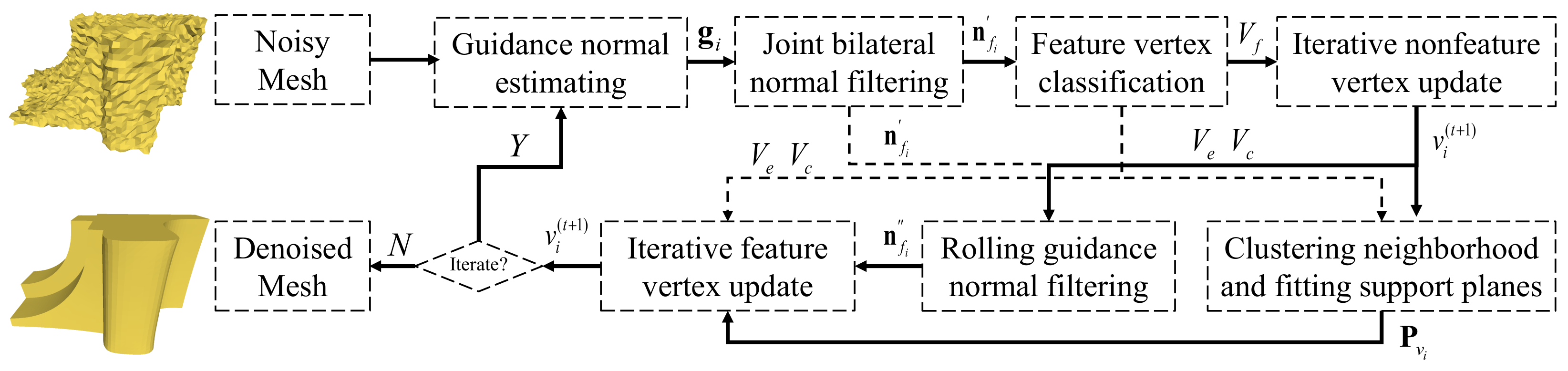
In summary, most of the current algorithms can remove the noise on the surface of the model, but the structure retention and restoration effect are still not satisfactory. The feature classification method based on NVT is very sensitive to the disturbance of the normal, which makes it impossible to classify feature points from the noisy model accurately. Our goal was to classify feature points accurately, preserve and restore the scene structure of the model when denoising, and avoid introducing pseudo features into the denoised model. More specifically, in this paper, we first apply joint bilateral filtering to the face normals, using the robust guidance normals; afterwards, classifying the feature points accurately by using the filtered facet normal; finally, removing noise using the anisotropic vertex denoising strategy with a local geometric constraint to retain the scene structure features of the model and avoid pseudo features.

3. Methodology

We proposed a 3D mesh model denoising algorithm based on feature point classification and anisotropic vertex denoising considering scene structure characteristics. The flowchart of our algorithm is illustrated in Figure 1. The symbols used in the article are shown in Table 1.

3.1. Facet Normal Filtering

In this section, we introduce a facet normal filtering method considering corner features.

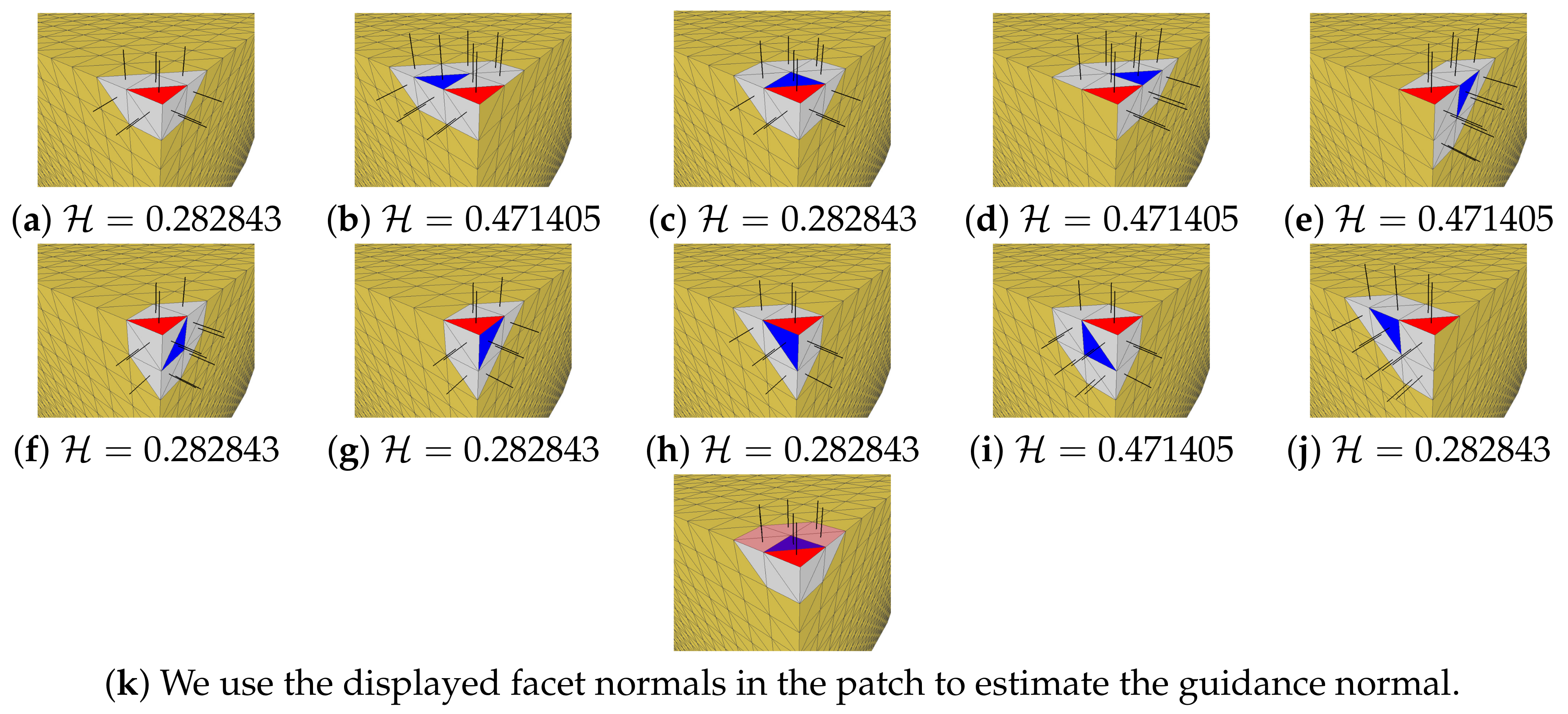
3.1.1. Guidance Normal Considering Corner Features

Given a target noisy 3D mesh model, our goal is to filter facet normals using estimated guidance normals, similarly to the GMNF method [5]. For the m t h patch P f i m of the face of interest f i , we measured the consistency of its normals using the function:
H ( P f i m ) = D ( P f i m ) * R ( P f i m ) ,
where D ( P f i m ) measures the maximum difference between two face normals from the patch:
D P f i m = max f j , f k P f i m n j n k
and R ( P f i m ) is a relative measure of edge saliency in the patch:
R P f i m = max e j E m φ e j ε + e j E m φ e j ,
where ε is a small positive value used to avoid division by zero, E m is a set of mesh edges with both incident faces contained in the m t h patch P f i m of face f i , and φ ( e j ) measures the saliency of an edge e j using the difference between the normals of the two incident faces f j 1 , f j 2 :
φ e j = n j 1 n j 2 .
Note that a small value of φ ( e j ) indicates similar face normals within the patch, while a small value of R ( P f i m ) indicates similar saliency among all interior edges of the patch.
However, after selecting a patch according to the consistency measures H , for a face of interest occupying the entire angular position, the GMNF method [5] cannot obtain a suitable patch, and its calculated guidance normal will lead to incorrect guidance. For a convenient explanation, we take the clean model in Figure 2 as an example, where red is the face of interest, blue is the center face of the corresponding patch, and the center face of the patch in Figure 2a is the current face of interest. Although the GMNF method [5] can choose the patch shown in Figure 2a,c,f–h or Figure 2i, this is possible because according to Equation (7) of GMNF [5], the consistency measures H of these patches are the smallest and are equal. However, regardless of which of these patches is selected, the calculated guidance normal cannot be used as the correct guide. This is because according to Equation (11) of GMNF [5], the guidance normal is the average normal of all faces in the patch according to the area weighting. The weights of all normals in the patch are almost the same (including normals that have a larger angle with the face of interest), which will cause incorrect guidance and eventually lead to the loss of corner features, as shown in Figure 3c.
To address this problem, we propose using a dual weight function to calculate the guidance normal of the selected patch, as shown in Equation (5). For the situation in Figure 2, when the face of interest selects a patch that crosses the fluted line or the corner feature, the guidance normal calculated by Equation (5) can filter out the internal normals that have a large deviation from the face of interest. Through the filtering effect of the parameter ρ , regardless of which patch with the most consistent internal normal is selected, we can obtain the correct guidance normal. For example, if the patch shown in Figure 2c is selected, we only need to use the isotropic normal shown in Figure 2k to calculate the guidance normal, which prevents the interest normal from being guided incorrectly. On the other hand, for areas that are flat or less variable, the normals inside the patch are more consistent and closer to the normal of interest, and the guidance normal calculated by Equation (5) is the same as that of Equation (11) of the GMNF method [5]. Therefore, the proposed dual weight function can adaptively obtain stronger and more accurate guidance normals.
The guidance normal g m corresponding to the m t h patch of the triangle of interest is:
g m = f j P f i m T i j A j n j f j P f i m T i j A j n j
T i j is a dual weight function. When the angle between the face normal of interest and the face normal n j is within the angle threshold ρ , T i j is set to 1; otherwise, it is set to 0. Here, ρ [ 0 , 1 ] is a threshold determined by the user, which is used to control averaging and has the default value ρ = 0.5 . The dual weight function makes the guidance normal more robust and avoids corner feature loss, as shown in Figure 3e. When the face of interest f i chooses the m t h patch, the guidance normal of the patch is regarded as the guidance normal of the face of interest; that is, g i = g m :
T i j = 1 if n j · n i ρ 0 if n j · n i < ρ
We compare the improved results with the GMNF method [5]. To conduct ablation studies, the comparative experiment in Figure 3 only differs in the method of calculating the guidance normal. The method of filtering the surface normal and updating the vertices is the same, and the number of iterations and other parameters are the same. In Figure 3 shows the CAD model with noise, Figure 3b shows the result of GMNF [5], and Figure 3c shows the result using the isotropic neighborhood to calculate the guidance normal. Figure 3d shows the denoising ultimately obtained by calculating the adaptive isotropic guidance normal. Figure 3e shows the denoising of g i calculated using our dual weight function Equation (6). The average normal angular differences between (b)–(e) and (a) are 21.0551 , 0.691454 , 2.1604 , and 0.652975 , respectively. It is clear that our method can avoid losing corner features in the process of denoising, and the result is closer to the original model. If directly using the isotropic neighborhood of the faces to calculate the guidance normals, for the non-flute corner area, the calculation of the guidance normal will not consider the larger neighborhood; it might be very close to the face normal of interest, and the facet normals in the non-featured areas will have a lower degree of filtering and a slower filtering speed, which will make it difficult to quickly denoise a flat or less variable area.

3.1.2. Joint Bilateral Normal Filtering

We perform the normal face filtering process using a joint bilateral filter similar to GMNF [5], which is a nonlinear filter, and it computes the output using the Gaussian kernels K s and the range kernel K r of the input as follows:
n f i = 1 W f i f j N F f i A j K s c i , c j K r g i , g j n j ,
where g i is a guidance normal of face f i , A j is the area of f j , c j is the centroid of f j , W f i = f j N F f i A j K s c i , c j K r g i , g j , and N F f i is the set of faces in a neighborhood of f i , which can be defined in a topological neighborhood or geometric neighborhood with reference to GMNF [5]. For meshes with highly non-uniform sampling, the size of the faces is not uniformly distributed. It may happen that the geometric neighbors of some faces are empty or that there are very few geometric neighbors. In this case, the geometric neighbors cannot fully express the geometric shape of the current triangle. If the number of geometric neighborhoods N F f i 3 , then N F f i takes the 1-ring topological neighborhood. The Gaussian kernel K s and the range kernel K r are Gaussian functions evaluated on the basis of the Euclidean distance:
K S c i , c j = exp c i c j 2 2 σ s 2 K r g i , g j = exp g i g j 2 2 σ r 2 ,
where σ s and σ r are variance parameters. The kernel values quickly fall off with increasing distance values.

3.2. Feature Point Classification

The accuracy of the feature point classification method based on the normal voting tensor depends on the reliability of the normals participating in the voting in the model. In order to reduce the unreliability caused by noise fluctuations, effectively improving the accuracy of feature classification, we calculate the normal voting tensor matrix of the vertices using the filtered facet normals in the previous step.

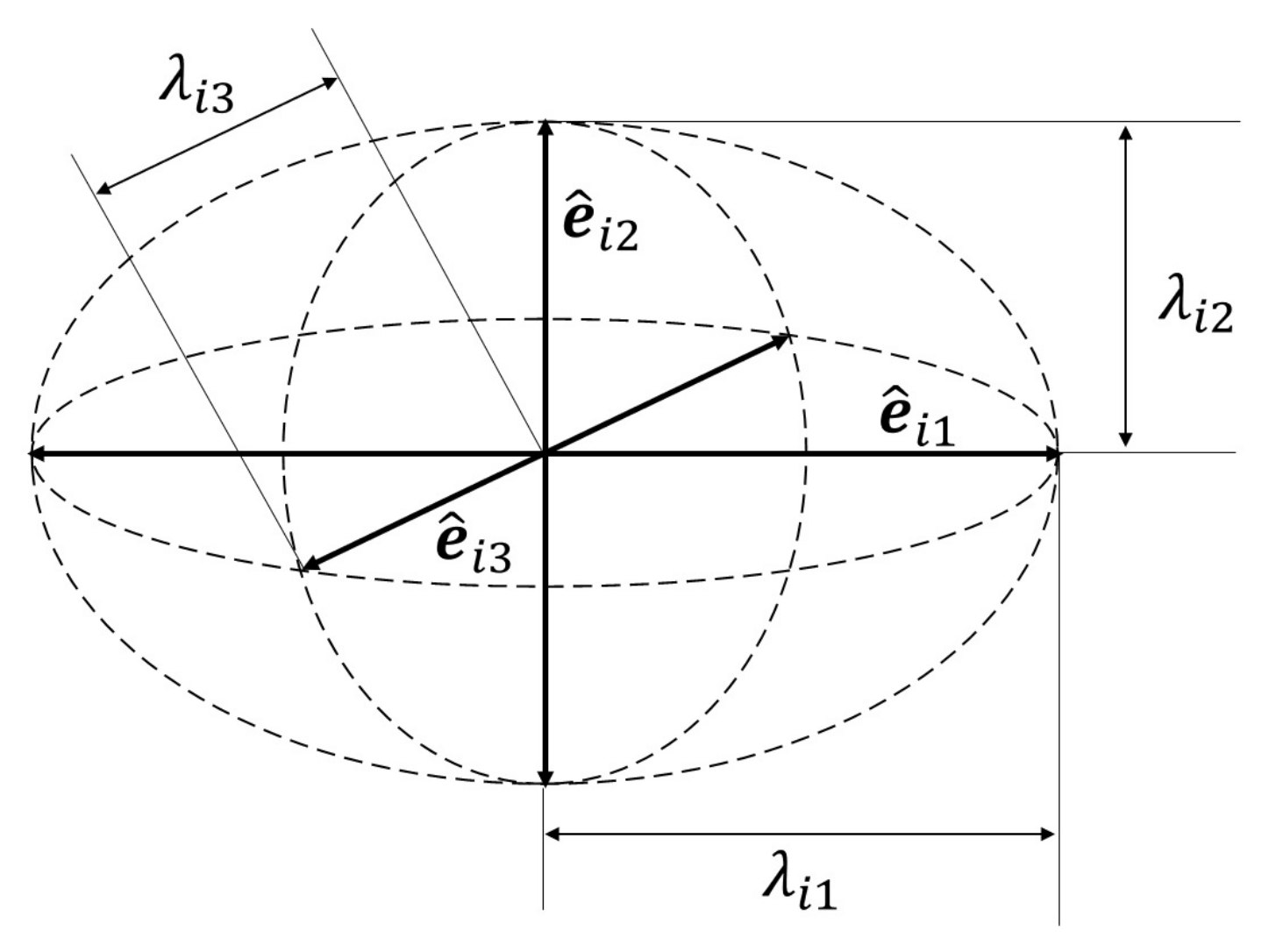
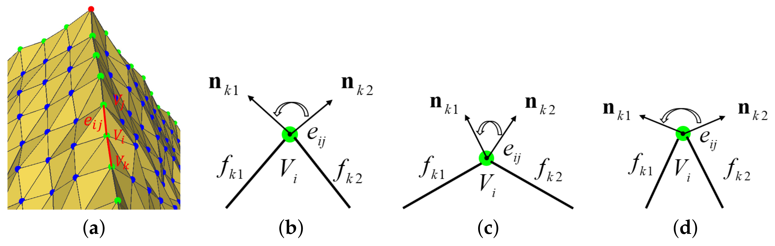
3.2.1. Feature Vertex Detection

N F v i is the set of faces in a neighborhood of the vertex v i . Consider v i and its nearest triangles f j , f j N F v i ; T v i is defined as a tensor voting matrix based on the normals at vertex v i of the triangular mesh [43], V f j is the normal voting component of the face f j , and the unit filtered normal of f j is n f j = ( x , y , z ) :
V f j = n f j n f j T = x 2 x y x z x y y 2 y z x z y z z 2
The normal voting tensor matrix T v i of a vertex v i on a mesh can be defined by the unit filtered normals of its neighbor triangle f j , f j N F v i :
T v i = f j N F v i μ f j V f j = f j N F v i μ f j n f j n f j T ,
where μ f j is the weight of triangle f j [8]:
μ f j = A f j A N F v i max m · exp m · c f j v i max m c f v i ,
where m is the number of facet rings around the vertex v i , A N F v i max represents the maximum area of all facet areas A f j from the vertex’s m t h -ring facets, c f j is the centroid of f j , and max c f v i denotes the maximum distance between the barycenters of the m t h -ring facets and the vertex v i . Facets with larger areas, closer topological connections, or smaller distances to the central vertex contribute more to tensor voting. T v i is a symmetric positive semidefinite and can be represented as
T v i = λ i 1 e ^ i 1 e ^ i 1 T + λ i 2 e ^ i 2 e ^ i 2 T + λ i 3 e ^ i 3 e ^ i 3 T = λ i 1 λ i 2 e ^ i 1 e ^ i 1 T + λ i 2 λ i 3 e ^ i 2 e ^ i 2 T + e ^ i 3 e ^ i 3 T + λ i 3 e ^ i 1 e ^ i 1 T + e ^ i 2 e ^ i 2 T + e ^ i 3 e ^ i 3 T
where λ i 1 λ i 2 λ i 3 0 are its eigenvalues and e ^ i 1 , e ^ i 2 , e ^ i 3 are the corresponding unit eigenvectors. According to the eigenvalues [47], the vertices can be classified into the face type, sharp-edge type, and corner type. Both sharp-edge-type and corner-type vertices are called feature vertices. The voting process produces a dense tensor map, which is then decomposed into two dense vector maps. In 3D, each voxel of these maps has a 2-tuple ( s , e ^ ) , where s is a scalar indicating feature intensity and e ^ is a unit vector indicating direction [43].
Face ( V f ): λ i 1 τ , λ i 3 λ i 2 τ , s = λ i 1 λ i 2 , e ^ = e ^ i 1 indicates the normal direction.
Sharp edge ( V e ): λ i 1 λ i 2 τ , and λ i 3 τ , s = λ i 2 λ i 3 , e ^ = e ^ i 3 indicates the tangent direction.
Corner ( V c ): λ i 1 λ i 2 λ i 3 τ , s = λ i 3 , e ^ is arbitrary.
τ is a feature detection parameter set by the user to ensure the quality of the recognized features. For a model with greater noise, the value should be set larger. We compute the normal voting tensor using the filtered normal to classify the feature points of the noisy model.

3.2.2. Weak Feature Recognition and False Feature Elimination

Isolated feature elimination [44]: If there are no other feature points in the n-ring (n has a default value of 3) neighbors of a feature point, the feature point is an isolated feature point, which can be removed.
Pseudo-corner feature elimination: The feature intensity can be represented by the feature value of the vertex tensor matrix. The feature intensity of each feature point is not necessarily the same. In the same model, the feature intensity of the feature corner point is greater than the feature edge point, and the greater the feature intensity is, the more obvious the feature. If there are two adjacent corner points, the feature intensity s of the true corner feature is larger than that of the false corner feature.
Weak feature point recognition: The direction vector e ^ of the shape edge points in the direction of the side line, as shown in Figure 4; the positive direction of e ^ is displayed in red, and the reverse direction is displayed in blue. If the non-feature point has two neighboring feature points and the vector formed by this point and the two feature points is within a certain angle of the direction vector of the corresponding feature point, we set it to 30 ; then, the non-feature point is recognized as a weakly shaped edge point. The vertex pointed to by the arrow in Figure 4b is not successfully recognized; according to weak feature recognition, in (c), we recognize this as a feature point.

3.3. Anisotropic Vertex Update

Since we classified the vertices, we need to consider different features of the vertices distributed in different positions. For the update of the non-feature points, we consider the average pulling force of the neighbor filtered normal to it. For the feature points, in addition to the average tensile force of the neighbors filtered normal to them, since we first denoise the non-feature area so that the flat supporting neighborhood on both sides of the feature edge can describe the edge geometry more accurately, we consider the tension of the supporting neighborhood point set (which is fit to obtain the supporting plane) of the feature point.

3.3.1. Non-Feature Vertex Update

The neighborhood of a vertex is important information for estimating the feature of a vertex. The traditional neighborhood of an interest vertex is used to indiscriminately search for the K-ring neighbors or geometric neighbors. In the high-frequency area and the cross-feature area, some neighborhood faces and vertices differ greatly from the features of the interest vertex. When the neighborhood surface normal acts on the interest point, it easily causes the feature to be oversmoothed. Therefore, for non-feature points located in a flat area, we use the isotropic neighbors of the non-feature points to achieve efficient denoising and feature retention. We choose isotropic geometric neighbor faces to preserve the geometrical neighborhood. We adopt the iterative scheme from [4] for the non-feature vertex update:
v i ( t + 1 ) = v i ( t ) + 1 N F f v i i s o t f k N F f v i i s o t n f k n f k c k ( t ) v i ( t ) ,
where v i ( t ) is the set of original vertex coordinate, ( t ) represents the t t h iteration, n f k is the filtered normal of face f k , c k ( t ) is the centroid of face f k , and n f k · n v i > ρ , where ρ defaults to 0.6. c k is the centroid of f k . N F v i i s o t is the set of isotropic neighbor faces of vertex v i , and n i is the normal of vertex v i .
In Figure 5, we use different neighborhoods to update non-feature points, and update feature points using all the neighborhoods just like GMNF [5]. As shown, with isotropic neighborhoods, corrugated lines and corners can be better preserved during noise removal. For the non-feature points near the feature, isotropic neighborhoods can reduce the influence of the vertices near the feature line from the triangle on the other side of the corrugated line and prevent the step corners from being rounded and blurred, as shown in Figure 5c. On the other hand, for flat non-characteristic areas, there is little difference in using isotropic neighbors; for noisy non-characteristic areas, using isotropic neighborhoods can reduce the negative influence of noise triangles and make local areas tend to become flat more quickly.

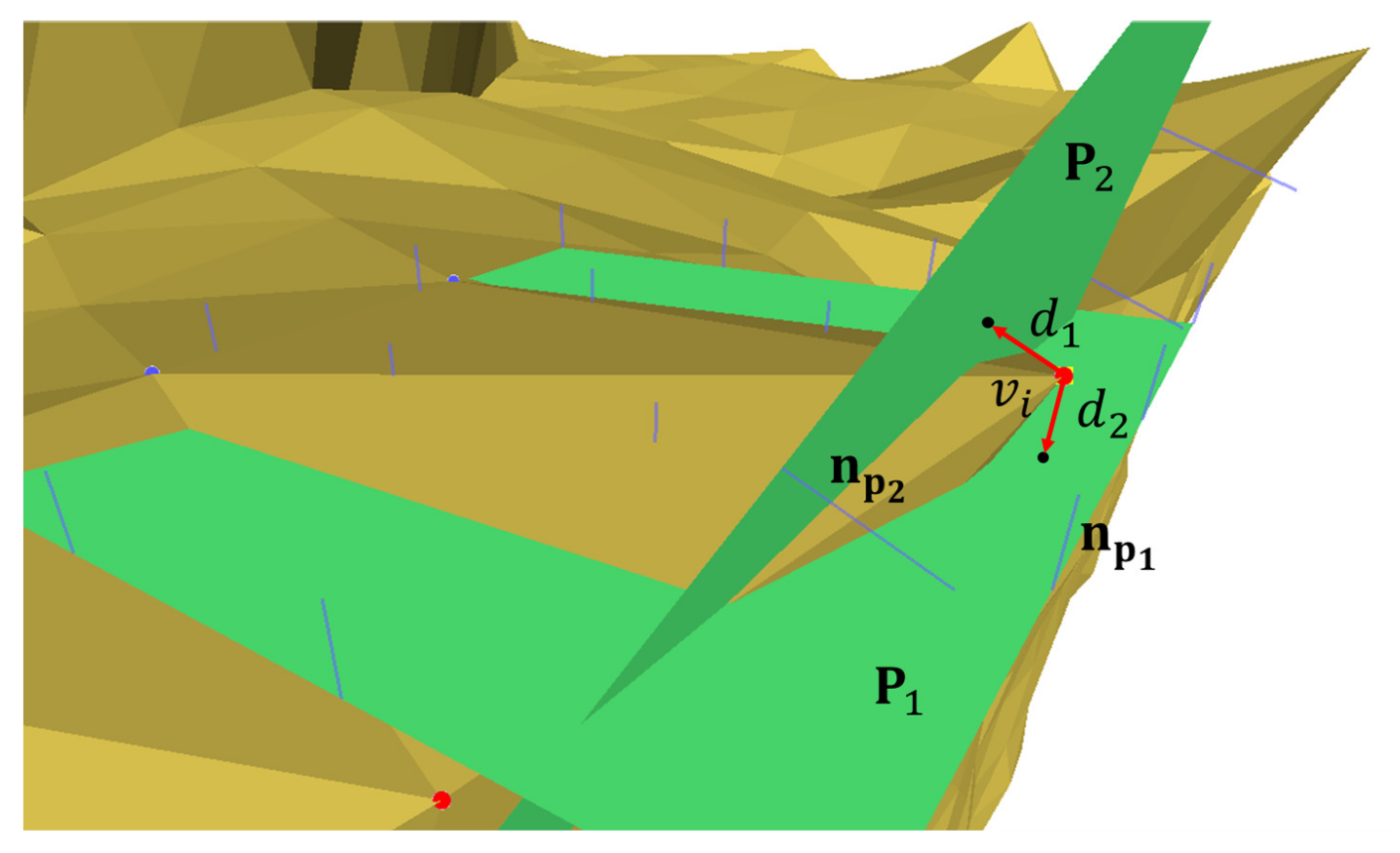
3.3.2. Feature Vertex Update

(1) Clustering the supported neighborhood of the feature vertex.
The positions of the feature points are affected by their support areas, which can fit the corresponding local support plane, and the local support planes work together to form a feature line or a feature angle. We cluster the support neighborhood of feature point using its eigenvector of tensor matrix. Since the tensor matrix of the vertex is a symmetric and positive semidefinite matrix [45], the eigenvectors of the matrix are orthogonal to each other, corresponding to the main direction of the ellipsoid, and the eigenvalues encode the size and shape of the ellipsoid, as shown in Figure 6.
The directions of the three feature vectors e ^ i 1 , e ^ i 2 , and e ^ i 3 do not necessarily satisfy the right-hand rule, nor do they all point from the model surface to the outside of the model. As shown in Figure 7a, red represents e ^ i 1 , green represents e ^ i 2 , and blue represents e ^ i 3 . For non-feature points, e ^ i 1 does not necessarily point to the outside of the model, and it may be opposite to the normal of the vertex. For shape edge points, e ^ i 1 and e ^ i 2 may be in the opposite direction from the normals of the region elements adjacent to both sides of the edge (we call the feature point the “supporting neighborhood”). For feature corners, the directions of e ^ i 1 , e ^ i 2 , and e ^ i 3 may also be opposite to the normal directions of their supporting neighborhoods. We use the vertex normal to correct the directions of e ^ i 1 , e ^ i 2 , and e ^ i 3 . When the angle between the eigenvector and the normal of the point is greater than 90 , it is reversed. The corrected result is shown in Figure 7b.
At this time, the eigenvectors e ^ i 1 and e ^ i 2 of the shape edge point voting matrix are consistent or close to the orientation of the support neighborhoods; then, we can use its feature vector to cluster the vertices of the support neighborhoods. They are clustered into two categories close to e ^ i 1 and e ^ i 2 , namely C i 1 and C i 2 . For the corner points, we can similarly cluster their supporting neighborhoods into three categories close to e ^ i 1 , e ^ i 2 , and e ^ i 3 , named C i 1 , C i 2 , and C i 3 . The clustering results (green) after denoising the non-feature vertices are shown in Figure 7c. Since the positions of the non-feature points were updated, the noise in these areas was reduced. At this time, using them to fit the plane can yield a more accurate plane that fits the model surface. If the number of vertices of a certain cluster is less than 2, it is considered unreliable and does not constitute a support plane. Each support plane has a pulling force for the feature point of interest, and this pulling force is defined as Δ v i 2 .
(2) Rolling guidance normal filtering for the neighbor facet normal.
After updating the non-feature area, we need to recalculate the filtered normals of the neighboring faces of the feature points. In the feature classification step, the geometric features with larger scales are identified as shape edge points and corner points. When removing noise, we need to retain the larger geometric features locally. Inspired by the RGNF [29] method, we use the last filtered normal as a new guidance signal to filter the neighbor facet normals of the feature points to remove small-scale noise and retain large-scale structural features. It is similar to Equation (7) in Section 3.1.2, and the filtered face normal is:
n f i = 1 W f i f j N F f i A j K s c i , c j K r n f i , n f j n j .
After updating the non-feature points, the centroid and normal of the face will be updated. n j is the current normal of face f j , and n f i is the last filtered normal in the current iteration. The larger the difference between n f i and n f j is, the larger the scale of the feature, the smaller the value of K r , and the smaller the extent of filtering. In each iteration, more large-scale features are retained or restored. Figure 8 shows the comparison results of updating the feature points with different normals. Figure 8a shows the noisy SharpSphere model; Figure 8b shows the result of using the current normal to directly update the feature points without filtering the normals again, which makes it difficult to restore the geometric features of the model; Figure 8c shows the result of using the guidance normals to update the feature points without filtering the normals again, which means the guidance normal will introduce pseudofeatures; Figure 8d shows the result of directly updating the feature points with the last filtered facet normals in Equation (7), where the edges may be incorrectly connected and some geometric shapes will be lost; Figure 8e update feature points using a approximate faltered normal n f i in Equation (14), where n f i is replaced by the guidance normal g i and then updating the feature points, which loses some of the feature corners; and Figure 8f shows our result, obtained by using the filtered facet normal n f i in Equation (14) to update the feature vertices. Our results retain or restore more geometric features.
(3) Feature vertex update based on local constraints.
For the feature point set V e c = V e V c , we update the positions of V e c according to both the neighbor facet filtered normal and its neighbor normal fields. After updating the non-feature vertices, the model has more accurate flat areas, which can provide a more stable support plane for V e c .
For real noisy data, such as 3D reconstruction models based on oblique images and scan data, the current commonly used denoising methods often smooth details or sharp features because not all vertices are treated differently. The GMNF method also has the problem of introducing pseudofeatures. Our goal is to keep as much of the larger local features as possible in the local neighbors and avoid introducing pseudofeatures that are too sharp locally by controlling the strength of feature restoration.
We use the increase and decrease in the dihedral angle of the local sharp edges to reflect the smoothness and sharpness of the local features during feature point denoising. For models with no noise or low noise, local sharp edges can be distinguished by the normals of the triangles where the edges are located. Since the facet normal of the noise model is very sensitive to noise and unreliable, we can apply the accurate feature points to find the sharp edge, and the edge e i j V i , V j formed by two adjacent feature points V i , V j is treated as a local sharp edge. For example, in the case of Figure 9, its corresponding 2D section is shown in Figure 9b. The dihedral angle of an edge is defined as the angle of the facet normals on both sides. During the update of vertex V i , the sharp edge in Figure 9c may be smoothed. At this time, the dihedral angle of the edge e i j V i , V j decreases. We use the parameter β 1 to limit the value of dihedral angle reduction; it may also happen that the sharp edges in Figure 9d become spikes, in which case the dihedral angle of edge e i j V i , V j will become larger, and we use the parameter β 2 to limit the value of the dihedral angle increase. We use Equation (15) to update the feature points. When there is a local sharp edge that does not meet the constraints, the feature points are not updated to prevent local sharp edges being smoothed and sharp pseudofeatures being introduced.
We update the positions of the shape edge points according to both the neighbor facet filtered normal and its support neighbor fields. The positions of the feature points are first affected by the tensile force Δ v i 1 of the neighboring filtered facet normals, and the correction amount for this part is expressed by Equation (16). Second, the feature points are also affected by the support neighborhoods, and these two sides of the edge line correspond to the local support plane. The distance from these planes produces a second part of the tensile force Δ v i 2 . The correction amount for this part can be expressed by Equation (17), as shown in Figure 10. Similarly, there are three local support neighborhoods and three planes for the corner points, and the correction amount due to the distance from these three support planes is also expressed by Equation (17):
v i ( t + 1 ) = v i ( t ) + α 1 Δ v i 1 + α 2 Δ v i 2
Δ v i 1 = 1 N F v i f k N F v i n f k n f k c k ( t ) v i ( t )
Δ v i 2 = p j P v i n p j v i ( t ) T + d j n p j
where ( t ) represents the t t h iteration, v i ( t + 1 ) is the new position of the current vertex v i ( t ) , α 1 and α 2 are user-set parameters, and α 1 + α 2 = 1 . The first correction amount α 1 Δ v i 1 in Equation (15) represents the pulling force of the filtered neighbor normals toward the feature point, and the second correction amount α 2 Δ v i 2 represents the pulling force of the support planes toward the feature point. p j P v i represents one of the support planes of the feature point v i , and d j is the distance from the feature point v i to the support plane p j .

4. Results

To verify the effectiveness of our algorithm, we utilized models using different data types, such as CAD data, 3D scan data and 3D models reconstructed from oblique images using the oblique photogrammetry method. The experimental content includes two parts: qualitative assessment and quantitative evaluation.
We contrast our method with the nine most closely related mesh denoising methods, which are the bilateral mesh denoising method (BM) [3], the noniterative, feature-preserving mesh smoothing method (NoIter) [27], the Fast method [28], the local scheme of bilateral normal filtering (BNF method) [4], the L0 method [23], the GMNF method [5], the ENVT method [45], the RoFi method [32] and the CPD method [9]. To make our comparison fair, some results are provided by these authors, and the unprovided data are obtained through experiments with the code provided by the authors. All these algorithms were implemented with the same software and hardware environments as ours, and we aimed to tune the parameters of each method to obtain the best results.

4.1. Parameter Tuning

There are eight parameters to be modulated in our algorithm, which are the two standard deviations σ s and σ r in the bilateral filter (Equation (8)), the number of iteration filtering facet normals ( n f i l t e r ), the total number of iterations, the number of times the vertices are updated in each iteration ( n u p d a t e ), the normal angle threshold ( ρ ) for calculating the guidance normal, and the feature point classification threshold ( τ ). The greater the noise is, the greater τ should be to identify the features in the noise. The dihedral angle constraint threshold ( β 1 and β 2 ) for updating the feature points is defined as 15 . The coefficients of the constraint terms ( α 1 and α 2 ) when updating the feature points are defined as α 1 = 0.8 . When the flute structure of the model is dominant, α 1 can be reduced to better restore the local geometric structure. Our parameter settings refer to the GMNF method, and σ s is set as the average distance between neighboring face centroids across the whole mesh [4]. For all results in this paper, we employ geometric neighborhoods for applying the filter unless stated otherwise. σ r controls the influence of the normal deviation; the larger the value is, the greater the degree of smoothing. With a large number of experiments, and as suggested in the GMNF method [5], we can set the following thresholds: r [ 2 σ s , 3 σ s ] , σ r [ 0.3 , 0.6 ] , n f i l t e r [ 1 , 75 ] , n u p d a t e [ 1 , 30 ] , τ ( 0 , 1.5 ] .

4.2. Qualitative Assessment Experiments

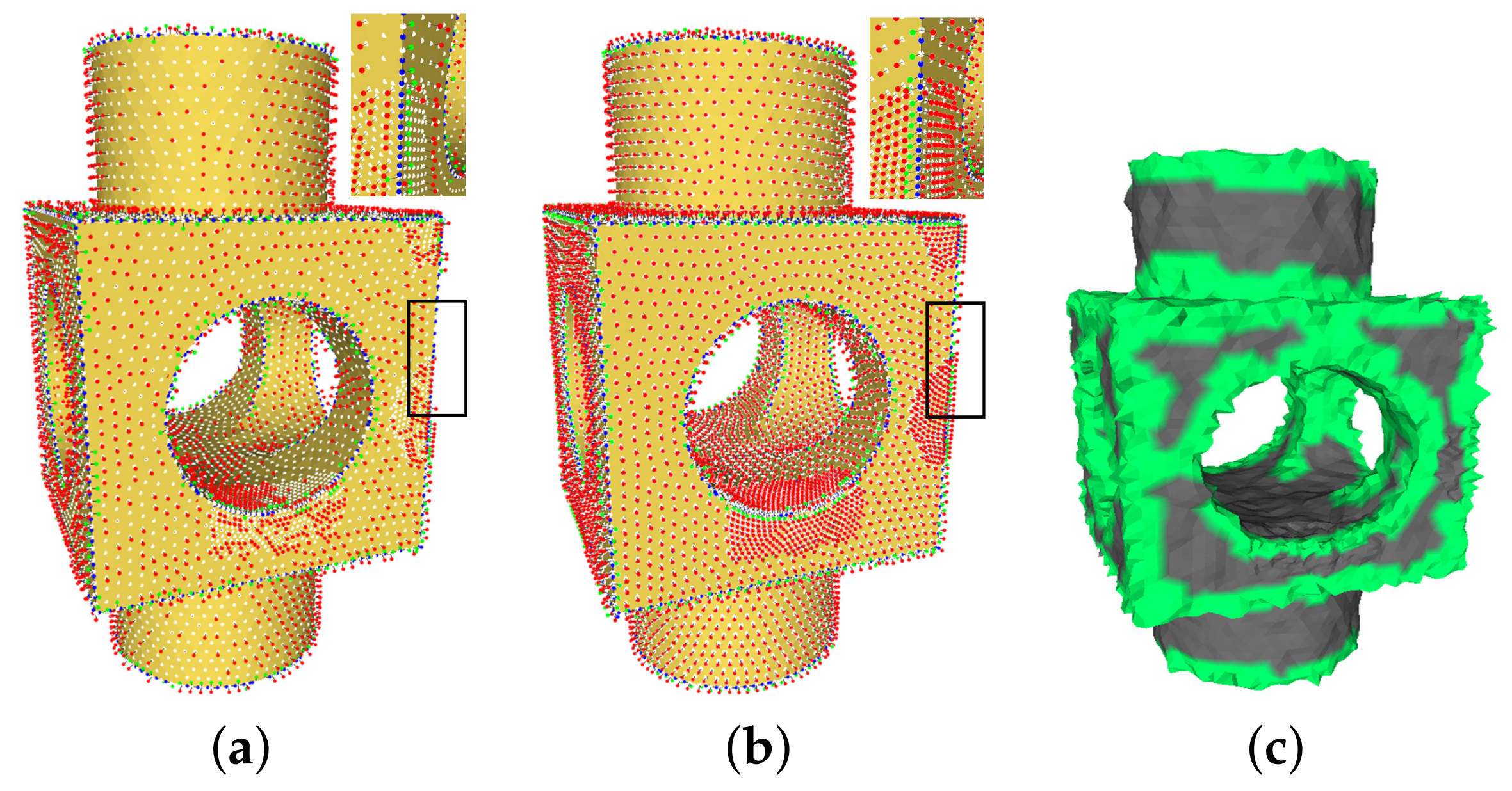
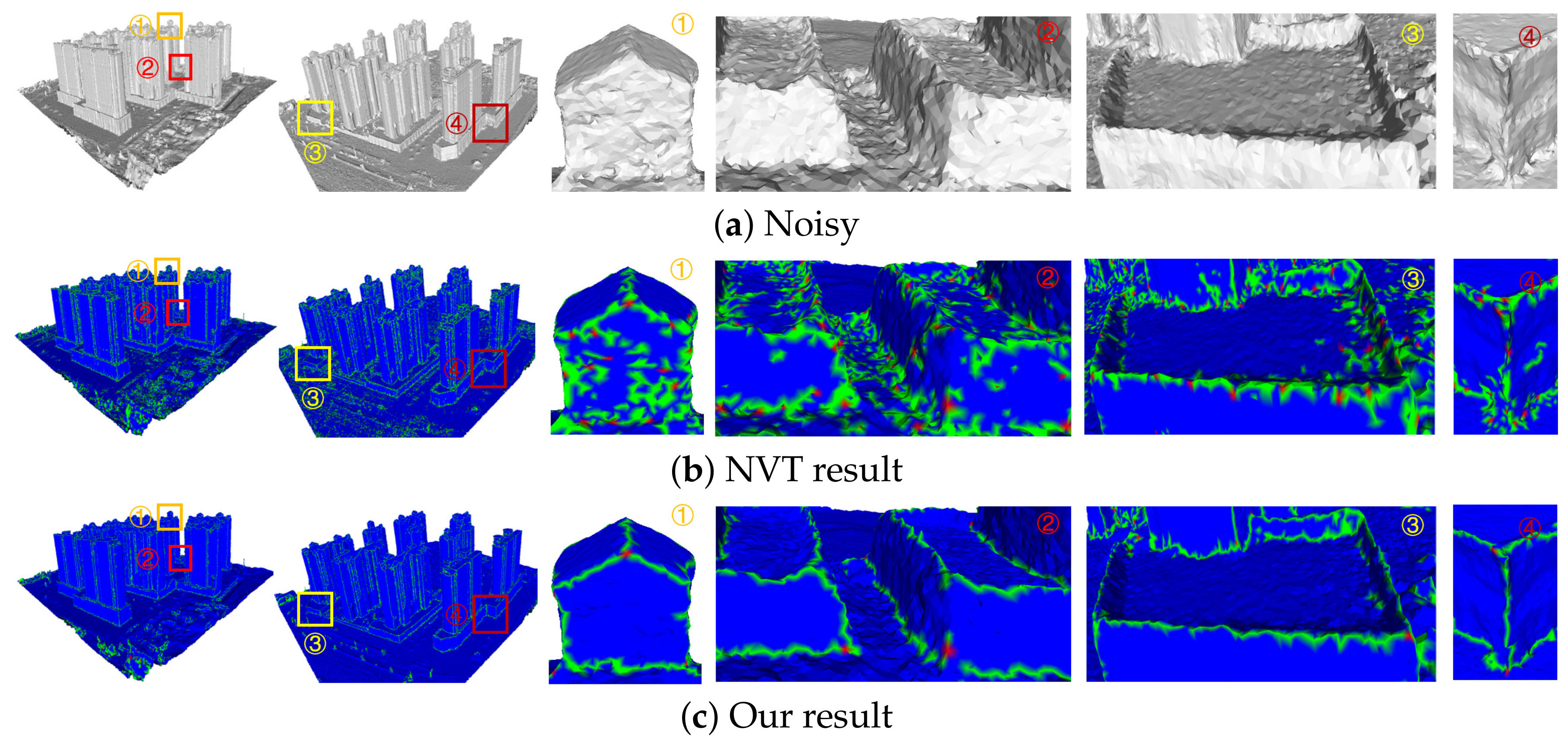
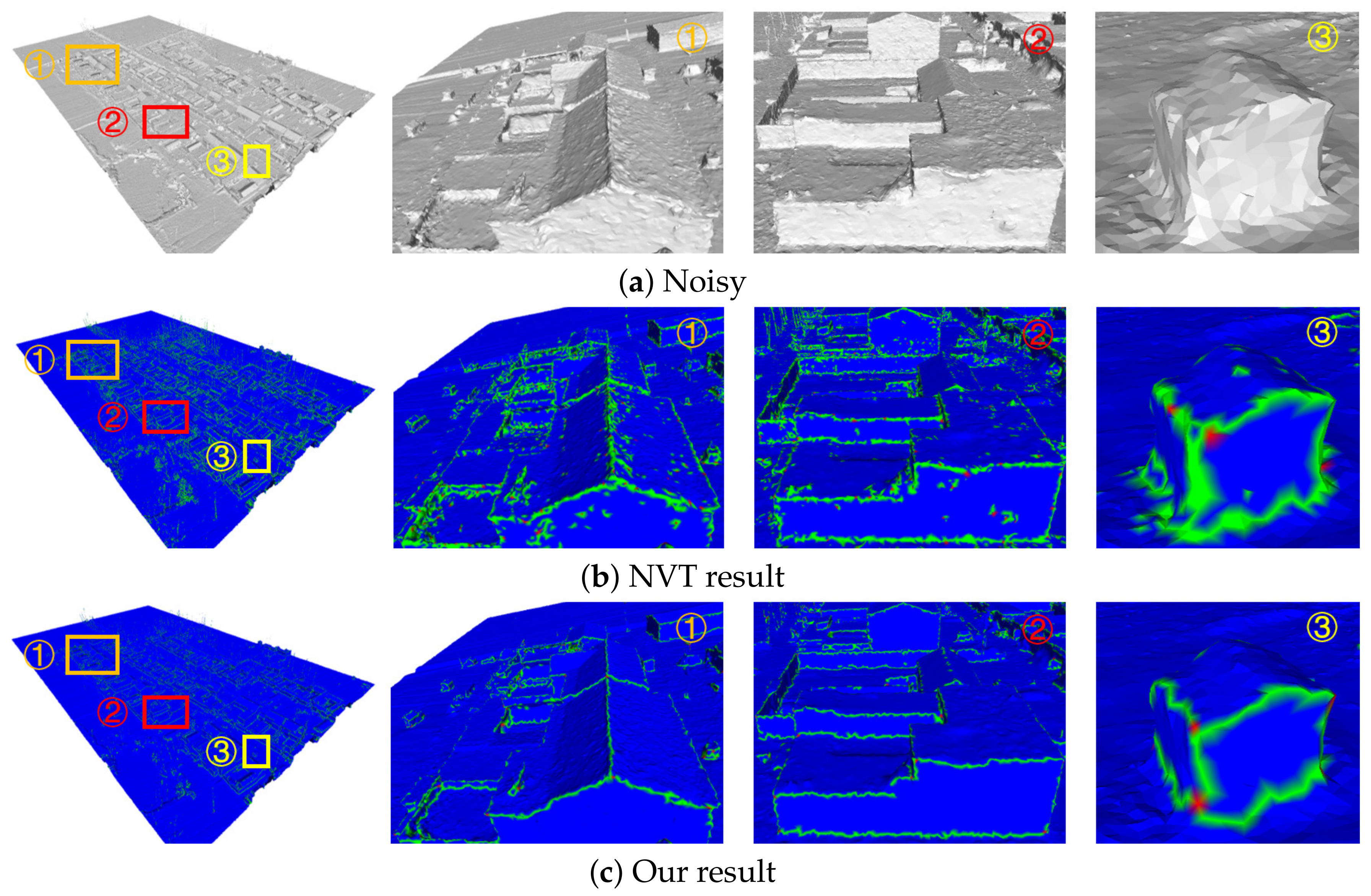
4.2.1. Qualitative Comparison of the Feature Vertex Classification Results

We classify the feature points in the noisy model according to our improved NVT method in Section 3.2.2. We contrast the feature vertex classification results with NVT on five different noisy models in Figure 11, Figure 12 and Figure 13, namely (1) a CAD model with Gaussian noise (the first line in Figure 11 and the fourth line in Figure 11; (2) a CAD model with random Gaussian noise (the second line in Figure 11; (3) a CAD model with impulse noise (the third line in Figure 11); (4) a real scan model (the fifth and sixth line in Figure 11); and (5) a real 3D model of oblique image reconstruction (Figure 12 and Figure 13). The noise intensities from the first line to the fourth line in Figure 11 are, respectively: σ e = 0.4 l e , σ e = 0.4 l e , σ e = 0.5 l e , σ e = 0.3 l e , where l e is the average edge length. The non-feature points, feature edge points and feature corner points are colored in blue, green and red, respectively, in the feature classification results.
As shown in Figure 11, the NVT method could not accurately classify the feature points of a noisy model regardless of whether it was Gaussian noise, random noise or impulse noise; for local regions with uneven sampling, such as the Block model, the NVT method could not correctly classify the feature points. However, our improved NVT method can accurately classify feature points from non-uniformly sampled regions. For the real scan models with low noise intensity, as shown in Figure 12, even if the noise intensity is not large, the NVT method cannot accurately classify the feature points. In contrast, our results can extract accurate structural features from real data with low noise intensity. For the 3D model generated by oblique images, as shown in Figure 12 and Figure 13, in the partially enlarged images (regions 1 and 2 in Figure 12 and Figure 13), the partially flat regions have no geometric structure but were mistakenly identified as structural features. By comparing the overall feature extraction effect, it can be seen that our method can obtain more accurate and comprehensive features than the NVT method.

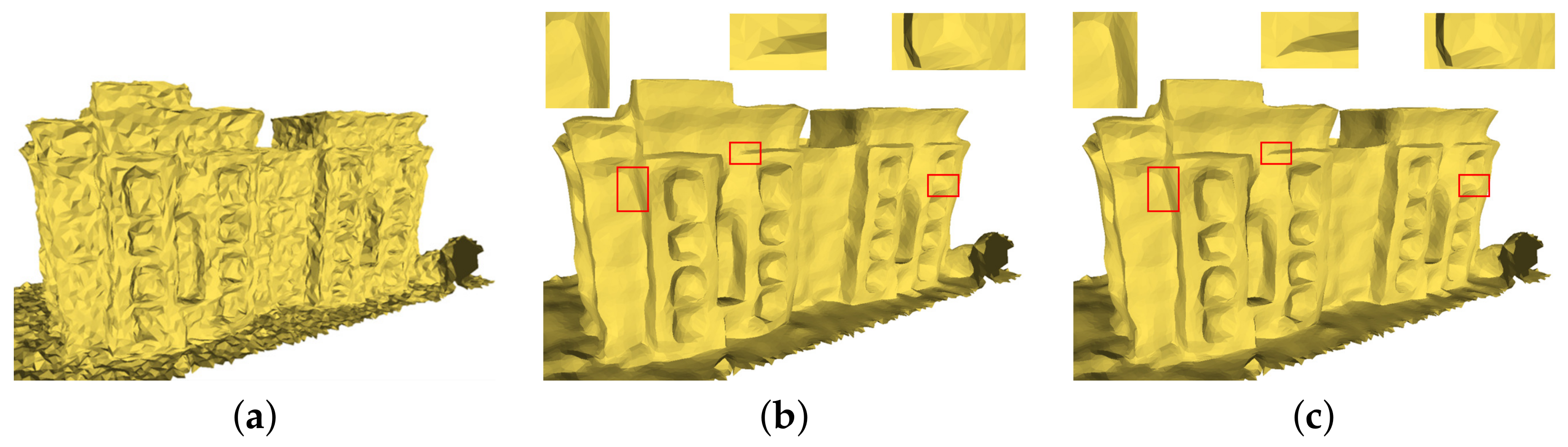
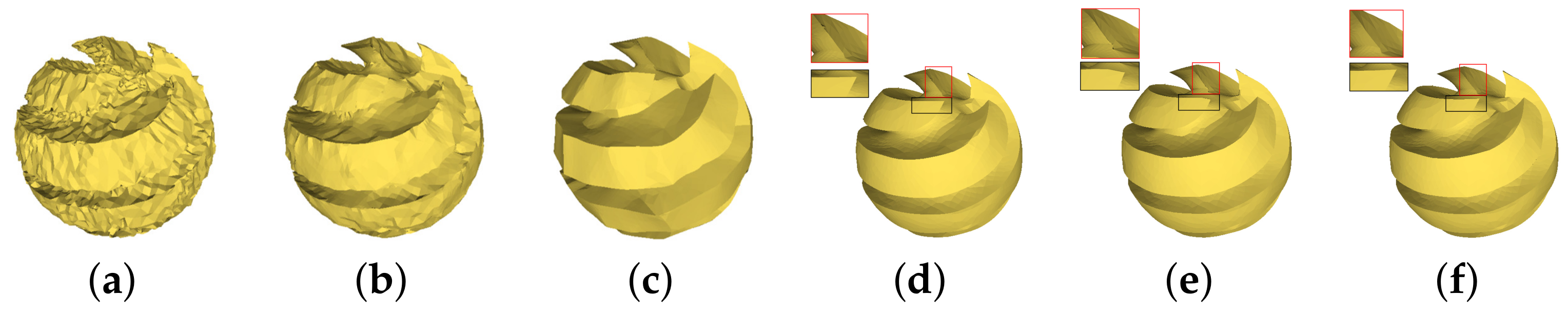
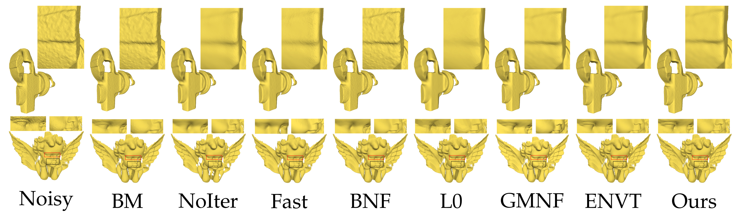
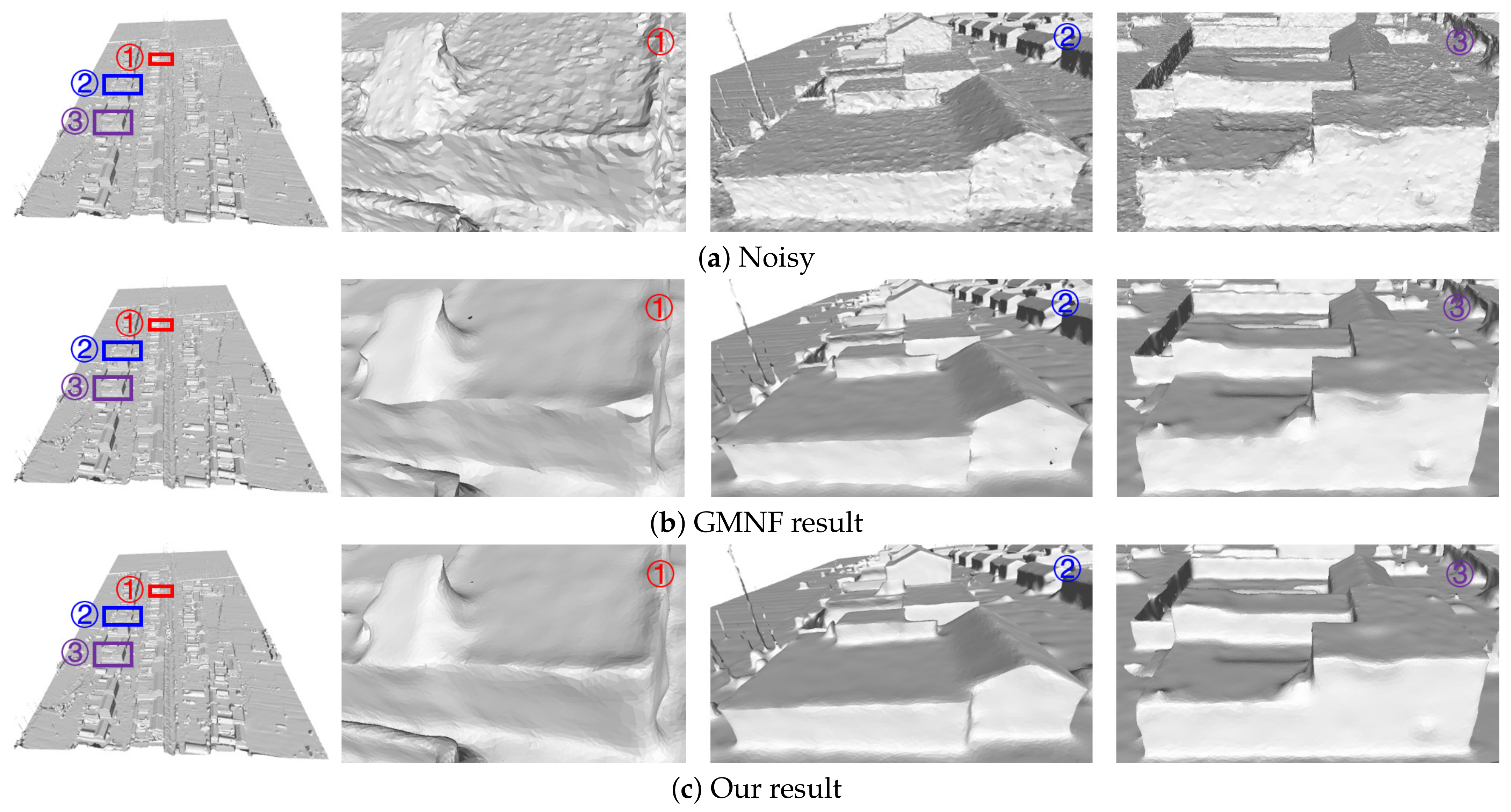
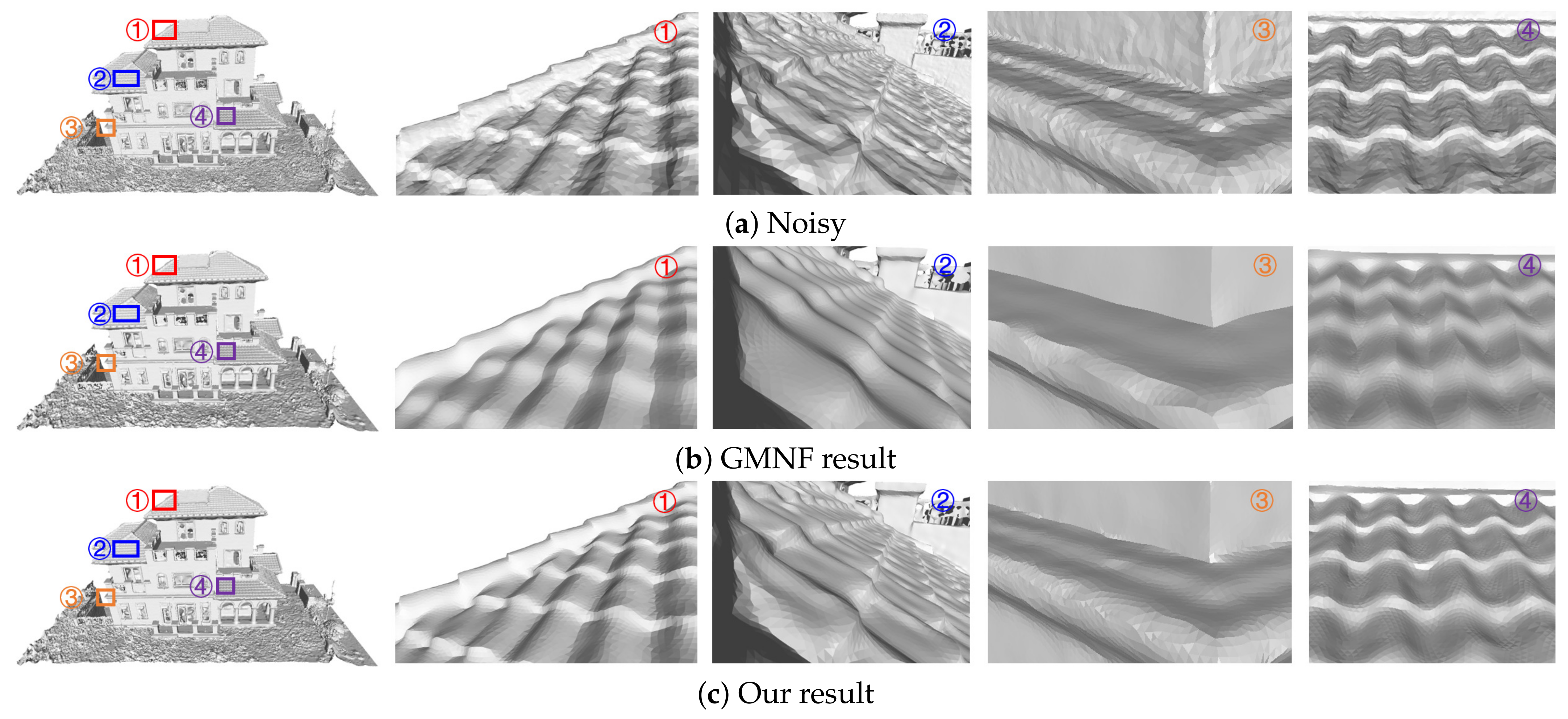
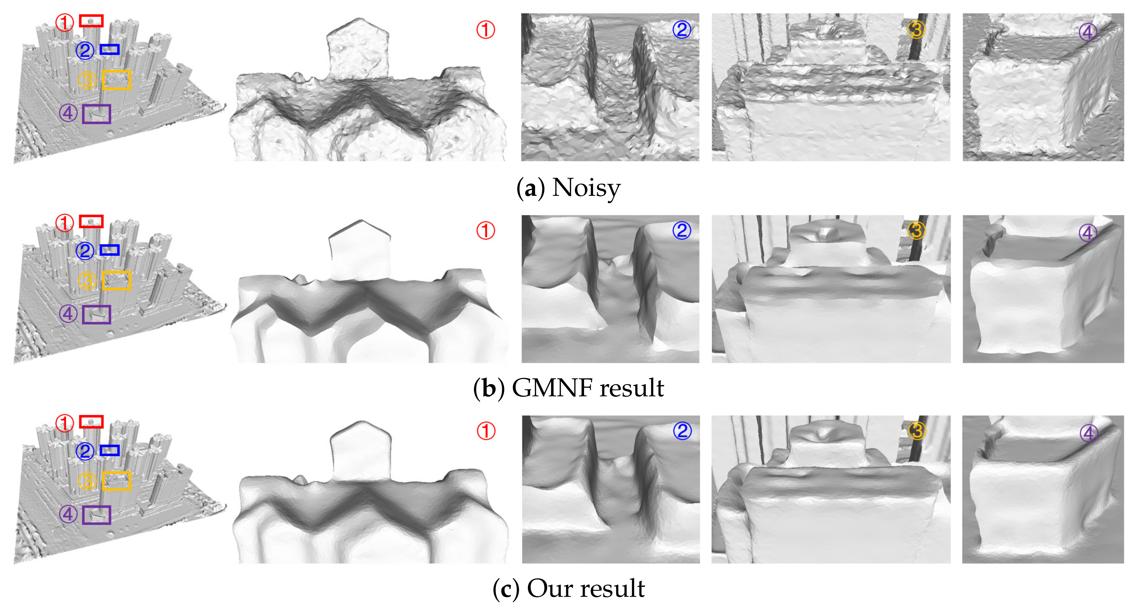
4.2.2. Qualitative Comparison of the Mesh Denoising Results

We show the comparison of the denoising results for the CAD model in Figure 14, the real noise of the scanning model in Figure 15, and the real noise of the oblique image reconstruction model in Figures 17–19, and compared the denoising results of nine popular algorithms.
In Figure 14, from top to bottom are the denoising results of Block, SharpSphere, Fandisk, Cube, Twirl and Julius model. In Figure 15, from top to bottom are the denoising results of angle and iron model. Note that to make a fair comparison, we enumerated the dense sample set in the parameter space of each method and selected the best result from the sample parameters. Some results of the algorithm (such as GMNF [5], ENVT [45], RoFi [32] and CPD [9]) are provided by the author. By analyzing and comparing the results, we can obtain the conclusions below.
First, our method performs well in preserving or restoring the characteristics of the noise model. The Block model, the SharpSphere model and the Twirl model in Figure 14 all have sharp corners and some curved edges. It can be seen from the local magnification and comparison that our results accurately remove all noise of the Block model while retaining rounded edges and truly restore the corners; retain the smooth continuous surface and sharp corners of the SharpSphere model; and rarely make the sharp corners of the Twirl model thicker or thinner. Our results better retain angled lips of the angle model in Figure 15. Compared with the prevalent methods, in addition to effectively eliminating noise, our method can more accurately retain the feature edges of the noise model.
Second, our method does not easily introduce pseudofeatures. For the Fandisk model in Figure 14, our result accurately removes all noise and does not produce any false features in the umbilical region, while retaining sharp features and corners; the similar results are shown in the nose of the local enlarged area of the iron model in Figure 15. However, the results for the L0 method [23], GMNF method [5] and RoFi method [32] introduced pseudofeatures on the originally smooth transition surface.
Third, our method is less sensitive to the sampling rate and sampling irregularities. The Cube model and the Block models in Figure 14 have partial irregular sampling. From the perspective of partial placement, our method can produce more ideal results while preserving the geometric features of different sizes.
Fourth, our method is relatively stable and has a certain degree of robustness. In contrast to the CPD algorithm [9] in Figure 16, we did not introduce convex points on the surface of the model. The CPD method [9] uses the vertex normals to calculate the normal tensor voting matrix and uses the normals of the vertices to update the vertex position. However, the normals of the vertices in the noise are very unreliable, which results in more common drifting spots.
Fifth, our algorithm can consider the structural characteristics of the scene. The 3D models reconstructed based on oblique images, such as building models, have a very rich linear scene structure. We removed the noise on the surface of the three groups of models (the Village model in Figure 17, the Villa model in Figure 18, and the City model in Figure 19) and partially magnified the prominent structures in them compared with the GMNF method before improvement. By comparing the overall display effect, it can be seen that both the GMNF algorithm and our method can smooth and remove the noise on the surface of the model. However, the GMNF algorithm sharpens the scene structure of the model as a whole, as shown in the partial regions in Figure 17 and Figure 19. In addition, it can be seen from the partial magnified area of the Villa model in Figure 18 that our algorithm can consider the structural features of the scene and preserve the geometric structure of the building in the model, such as the corners of the tiles and walls of the building.

4.3. Quantitative Evaluation Experiments

From the above visual comparison, we can infer that our method is generally better than the state-of-the-art methods. To distinguish them objectively, we compared the denoising results with the ground-truth model and measured the fidelity of the denoising results. We evaluate the denoised mesh quality with the following metrics: (1) The average normal difference N m e a n (in degrees) between the facet normals of the denoised mesh and the ground-truth facet normals; (2) The maximum distance D m a x and the average distance D m e a n from the resulting mesh vertices to the ground-truth mesh surface. We compare these metrics on different models and illustrate them via statistical data (see Table 2, Table 3 and Table 4).

4.3.1. Quantitative Comparison of the Normal Difference

It can be seen from Table 2 that for most models, the results obtained by our algorithm are generally less different from the surface normals of the original model. However, the SharpSphere model is an exception because it restores sharp features and weakens the dihedral sharpening constraint. In this way, although the sharp features of the real mesh are successfully restored, sharp artifacts are also induced in the concave area of the SharpSphere model, resulting in a higher normal difference. The jointSharpEdges model processed by the L0 method [23] has a greater degree of denoising and a greater degree of smoothness, and its overall normal is closer to the original surface. However, it can be seen from the visualization results that due to excessive smoothing, it smooths the right angles, resulting in a loss of features. The same is true of the Julius model processed by the BNF method [4]. The degree of denoising is greater, and the overall result is closer to the original surface, but the eyes become blurred.

4.3.2. Quantitative Comparison Of Distance

For most of the models, our method achieves better results than the current popular algorithms, according to the maximum distance D m a x and average distance D m e a n from the resulting mesh vertices to the ground-truth mesh surface shown in Table 3 and Table 4. Among them, the normal line of the Julius model of BNF [4] denoising is closer to the original model, but the distance from the vertex to the original model is not the closest. This is because when more noise is removed, the model shrinks, and the average distance from the original model becomes larger. This is also true when our method denoises the cube model. As a result, the average normal of the model is closer to the original normal. However, due to the greater degree of denoising, the model shrinks as well, so the average distance is not the smallest.

4.3.3. Quantitative Comparison of Running Time

Table 5 provides the running time comparison for the shown examples, on a PC with an Intel Core i7-8550U CPU. The processing time of the algorithm is related to the number of iterations. Since the algorithm has many steps and each iteration has to perform a feature point classification, our denoising process is inferior in efficiency. This is the problem we are prepared to solve in the future.

4.4. Discussion

The qualitative and quantitative comparisons help in analyzing the capabilities of all comparison algorithms. It can be seen that the BM method [3] can denoise models with low noise intensity, such as scanning models, but it is not suitable for handling large noise, and the feature retention effect is not ideal. The smoothing effect of the NoIter method [27] is better, and it can handle low-intensity noise; the denoising ability decreases with the increase in noise intensity, it is suitable for processing scanning noise, and the feature retention effect is not ideal. The Fast method [28] is suitable for dealing with various types of noise, and the denoising ability is strong, which can retain features to a certain extent; the BNF algorithm [4] is suitable for processing various types of noise. It has a strong denoising ability and good feature retention performance; this basic algorithm is not ideal for non-uniform noise processing. The L0 algorithm [23] has a strong denoising ability and can yield a very smooth model. It retains large-scale structural features to a certain extent but may introduce false features to deal with non-uniform noise. The GMNF algorithm [5] has a strong denoising ability and can be retained to a certain extent or restore sharp features but often introduces false features, which may lose angular features, and it can handle non-uniformly sampled noise. The RoFi algorithm [32] has a strong denoising ability and can handle a variety of noise; fewer triangles are flipped, and the feature retaining ability is strong, but it may introduce false features. The CPD method [9] is unstable and easily causes flying spots on the surface of the model. Our algorithm can handle a variety of features, handle non-uniform noise, consider the structural features of the scene, and retain or restore features with strong reliability, and it does not easily introduce false features.
The comparison of qualitative and quantitative experiments helps in analyzing our algorithm intuitively and objectively. Comparing Table 2, Table 3 and Table 4 in the quantitative analysis, it can be seen that when it is necessary to move closer to the surface of the original model, most of the algorithms can achieve this by increasing the degree of denoising, but this is often accompanied by the loss of the structural features of the model, such as in the BNF algorithm and L0 algorithm. We show that our approach outperforms the state-of-the-art methods in terms of N m e a n (average normal difference), D m a x (maximum distance difference) and D m e a n (mean distance difference) in the denoised mesh versus the ground-truth mesh. Comparing the qualitative analysis results, we can see that we retain more structural features. Through experiments on three typical 3D mesh model data sets with different noise, the experimental conclusions are as follows: (1) The improved feature classification method proposed in this paper is suitable for different noisy models. Compared with the original NVT method, our method reduces the number of false feature points and can classify more real structural feature points; (2) The denoising algorithm proposed in this paper can remove a variety of noise, deal with non-uniform noise, and retain and restore the structural features of the model. Compared with the original GMNF method, we take into account the corner features. Compared with the current popular denoising algorithms, our method can remove the noise on the surface of the mesh model while more realistically taking into account and retaining the structural features of the scene. At the same time, the false features are reduced. However, from the experiments, we also found that our method still has room for improvement. Our algorithm needs to set some parameters based on experience, and the parameter setting process is not sufficiently automatic; and our algorithm needs to classify and extract feature points and update the vertices step by step, which takes considerable time. In future research, the execution efficiency of the algorithm can be further improved, and more refined and faster 3D mesh denoising can be achieved.
The limitations of the algorithm are presented as follows. Firstly, when a detail with characteristic size D is sampled on the object surface and the noise of the sample is D/2 or larger, the limitations of the algorithm are: (1) the result of feature classification is not real. According to the Nyquist–Shannon theorem [48], in this case, the geometric sampling will appear as an aliasing phenomenon, and the geometric structure of the surface will be distorted, so the features obtained by our algorithm is the substitute of the real features; (2) The denoising results will lose the scene structure. Since denoising is an ill-posed problem, our algorithm cannot accurately recover the real structures from the distorted noise model; Secondly, our denoising method cannot deal with small holes in noisy meshes well. Figure 20c illustrates such an extreme case, where the noise around the holes is not removed as expected. However, small holes do not affect the classification of feature points, as shown in Figure 20b. In addition, in Figure 16, the denoising result of the low-intensity noisy model is almost not affected by small holes.

5. Conclusions

Noise removal in 3D model denoising is a research hotspot in the field of 3D reconstruction. The denoising algorithm based on bilateral filtering does not fully consider the structural features in the scene, resulting in the structural features of the optimized model being smoothed, missed and overly sharp. Feature classification helps in performing anisotropic mesh denoising that takes the geometric structure into account. However, the feature classification method based on the NVT is very sensitive to noise, and it is difficult to accurately classify the structural feature points of the model in a noisy scene. This research makes full use of accurately classified structural feature points and proposes an anisotropic mesh model denoising algorithm. It has three main parts: (1) The filter facet normals of the mesh; (2) A classification of the feature points based on the improved NVT method; and (3) The anisotropic update vertices of the mesh.
In general, we propose a 3D mesh Pre-processing method based on feature point classification and anisotropic vertex denoising considering the scene structure characteristics. Compared with the GMNF method and the current popular denoising algorithm, this study’s method achieves the following three goals: (1) Improving the estimation method of the guided normal and improving the robustness of the GMNF method to filter the normal to a certain extent; (2) Improving the accuracy of the classification feature points of the noise model (helping to accurately consider the real scene structure of the model); and (3) Retaining the geometric structure features to the greatest extent and reducing the pseudosharp line structure. This method provides a new solution for 3D model denoising.

Author Contributions

Conceptualization, Y.L.; methodology, Y.L. and W.Q.; software, Y.L. and W.Q.; formal analysis, Y.L., X.X. and W.Q.; investigation, Y.L.; resources, B.G. and X.X.; data curation, Y.L. and W.Q.; writing—original draft preparation, Y.L.; writing—review and editing, Y.L. and X.X.; visualization, Y.L. and W.Q.; supervision, B.G. and X.X.; project administration, B.G. and X.X.; funding acquisition, B.G. and X.X. All authors have read and agreed to the published version of the manuscript.

Funding

This research was funded by the National Natural Science Foundation of China, grant number 91,638,203; the Open Fund of Key Laboratory of Urban Land Resources Monitoring and Simulation, Ministry of Natural Resources, grant number KF-2018-03-052.

Institutional Review Board Statement

The study did not involve humans or animals.

Informed Consent Statement

The study did not involve humans.

Data Availability Statement

Not applicable.

Acknowledgments

We sincerely thank the anonymous reviewers for their comments and suggestions, which is crucial for this paper.

Conflicts of Interest

The authors declare no conflict of interest.

Abbreviations

The following abbreviations are used in this manuscript:
NVTNormal voting tensor
BMThe bilateral mesh denoising method [3]
NoIterThe noniterative, feature-preserving mesh smoothing method [27]
FastFast and effective feature-preserving mesh denoising [28]
BNFThe local scheme of bilateral normal filtering method [4]
L0Mesh denoising via L0 minimization [23]
GMNFGuided mesh normal filtering [5]
RoFiRobust and high fidelity mesh denoising [32]
CPDConstraint-based point set denoising [9]
ENVTMesh denoising based on normal voting tensor and binary optimization [45]

References

  1. Ham, H.; Wesley, J.; Hendra, H. Computer vision based 3D reconstruction: A review. Int. J. Electr. Comput. Eng. 2019, 9, 2394. [Google Scholar] [CrossRef]
  2. Zhao, W.; Liu, X.; Wang, S.; Fan, X.; Zhao, D. Graph-based feature-preserving mesh normal filtering. IEEE Comput. Archit. Lett. 2019, 1, 1. [Google Scholar] [CrossRef] [PubMed]
  3. Fleishman, S.; Drori, I.; Cohen-Or, D. Bilateral mesh denoising. In ACM Transactions on Graphics; Association for Computing Machinery: New York, NY, USA, 2003; pp. 950–953. [Google Scholar]
  4. Zheng, Y.; Fu, H.; Au, O.K.C.; Tai, C.L. Bilateral normal filtering for mesh denoising. IEEE Trans. Vis. Comput. Graph. 2010, 17, 1521–1530. [Google Scholar] [CrossRef] [PubMed]
  5. Zhang, W.; Deng, B.; Zhang, J.; Bouaziz, S.; Liu, L. Guided Mesh Normal Filtering. Comput. Graph. Forum. 2015, 34, 23–34. [Google Scholar] [CrossRef]
  6. Li, X.; Li, R.; Zhu, L.; Fu, C.W.; Heng, P.A. DNF-Net: A Deep Normal Filtering Network for Mesh Denoising. IEEE Trans. Vis. Comput. Graph. 2020, 70, 1. [Google Scholar] [CrossRef]
  7. Lu, X.; Deng, Z.; Chen, W. A robust scheme for feature-preserving mesh denoising. IEEE Trans. Vis. Comput. Graph. 2015, 22, 1181–1194. [Google Scholar] [CrossRef]
  8. Wei, M.; Liang, L.; Pang, W.M.; Wang, J.; Li, W.; Wu, H. Tensor voting guided mesh denoising. IEEE Trans. Autom. Sci. Eng. 2016, 14, 931–945. [Google Scholar] [CrossRef]
  9. Yadav, S.K.; Reitebuch, U.; Skrodzki, M.; Zimmermann, E.; Polthier, K. Constraint-based point set denoising using normal voting tensor and restricted quadratic error metrics. Comput. Graph. 2018, 74, 234–243. [Google Scholar] [CrossRef]
  10. Field, D.A. Laplacian smoothing and Delaunay triangulations. Commun. Appl. Numer. Methods 1988, 4, 709–712. [Google Scholar] [CrossRef]
  11. Vollmer, J.; Mencl, R.; Mueller, H. Improved Laplacian Smoothing of Noisy Surface Meshes. Comput. Graph. Forum 1999, 18, 131–138. [Google Scholar] [CrossRef]
  12. Taubin, G. A signal processing approach to fair surface design. In Proceedings of the 22nd Annual Conference on Computer Graphics and Interactive Techniques, SIGGRAPH 1995, Los Angeles, CA, USA, 6–11 August 1995; pp. 351–358. [Google Scholar]
  13. Desbrun, M.; Meyer, M.; Schröder, P.; Barr, A.H. Implicit fairing of irregular meshes using diffusion and curvature flow. In Proceedings of the 26th Annual Conference on Computer Graphics and Interactive Techniques, Los Angeles, CA, USA, 8–13 August 1999; pp. 317–324. [Google Scholar]
  14. Ohtake, Y.; Belyaev, A.G.; Bogaevski, I.A. Polyhedral surface smoothing with simultaneous mesh regularization. In Proceedings of the IEEE Proceedings Geometric Modeling and Processing 2000, Theory and Applications, Hong Kong, China, 10–12 April 2020; pp. 229–237. [Google Scholar]
  15. Zhang, H.; Van Kaick, O.; Dyer, R. Spectral Mesh Processing. Comput. Graph. Forum 2010, 29, 1865–1894. [Google Scholar] [CrossRef] [Green Version]
  16. Wang, P.S.; Liu, Y.; Tong, X. Mesh denoising via cascaded normal regression. ACM Trans. Graph. 2016, 35, 232. [Google Scholar] [CrossRef]
  17. Liu, L.; Tai, C.L.; Ji, Z.; Wang, G. Non-iterative approach for global mesh optimization. Comput.-Aided Des. 2007, 39, 772–782. [Google Scholar] [CrossRef] [Green Version]
  18. Wu, X.; Zheng, J.; Cai, Y.; Fu, C.W. Mesh Denoising Using Extended ROF Model with L1 Fidelity. Comput. Graph. Forum 2015, 34, 35–45. [Google Scholar] [CrossRef]
  19. Lu, X.; Chen, W.; Schaefer, S. Robust mesh denoising via vertex pre-filtering and l1-median normal filtering. Comput. Aided Geom. Des. 2017, 54, 49–60. [Google Scholar] [CrossRef]
  20. Liu, Z.; Lai, R.; Zhang, H.; Wu, C. Triangulated surface denoising using high order regularization with dynamic weights. SIAM J. Sci. Comput. 2019, 41, B1–B26. [Google Scholar] [CrossRef]
  21. Zhong, S.; Xie, Z.; Liu, J.; Liu, Z. Robust mesh denoising via triple sparsity. Sensors 2019, 19, 1001. [Google Scholar] [CrossRef] [PubMed] [Green Version]
  22. Ohtake, Y.; Belyaev, A.; Bogaevski, I. Mesh regularization and adaptive smoothing. Comput.-Aided Des. 2001, 33, 789–800. [Google Scholar] [CrossRef]
  23. He, L.; Schaefer, S. Mesh denoising via L 0 minimization. ACM Trans. Graph. (TOG) 2013, 32, 1–8. [Google Scholar] [CrossRef] [Green Version]
  24. Wang, R.; Yang, Z.; Liu, L.; Deng, J.; Chen, F. Decoupling noise and features via weighted L1-analysis compressed sensing. ACM Trans. Graph. (TOG) 2014, 33, 1–12. [Google Scholar]
  25. Tomasi, C.; Manduchi, R. Bilateral filtering for gray and color images. In Proceedings of the Sixth International Conference on Computer Vision (IEEE Cat. No. 98CH36271), IEEE, Bombay, India, 4–7 January 1998; pp. 839–846. [Google Scholar]
  26. Durand, F.; Dorsey, J. Fast bilateral filtering for the display of high-dynamic-range images. In Proceedings of the 29th Annual Conference on Computer Graphics and Interactive Techniques, San Antonio, TX, USA, 23–26 July 2002; pp. 257–266. [Google Scholar]
  27. Jones, T.R.; Durand, F.; Desbrun, M. Non-Iterative, Feature-Preserving Mesh Smoothing. In Proceedings of the ACM SIGGRAPH 2003 Papers, San Diego, CA, USA, 27–31 July 2003; pp. 943–949. [Google Scholar]
  28. Sun, X.; Rosin, P.L.; Martin, R.; Langbein, F. Fast and effective feature-preserving mesh denoising. IEEE Trans. Vis. Comput. Graph. 2007, 13, 925–938. [Google Scholar] [CrossRef]
  29. Wang, P.S.; Fu, X.M.; Liu, Y.; Tong, X.; Liu, S.L.; Guo, B. Rolling guidance normal filter for geometric processing. ACM Trans. Graph. (TOG) 2015, 34, 1–9. [Google Scholar] [CrossRef]
  30. Zhang, J.; Deng, B.; Hong, Y.; Peng, Y.; Qin, W.; Liu, L. Static/dynamic filtering for mesh geometry. IEEE Trans. Vis. Comput. Graph. 2018, 25, 1774–1787. [Google Scholar] [CrossRef] [PubMed] [Green Version]
  31. Li, T.; Wang, J.; Liu, H.; Liu, L.G. Efficient mesh denoising via robust normal filtering and alternate vertex updating. Front. Inf. Technol. Electron. Eng. 2017, 18, 1828–1842. [Google Scholar] [CrossRef]
  32. Yadav, S.K.; Reitebuch, U.; Polthier, K. Robust and high fidelity mesh denoising. IEEE Trans. Vis. Comput. Graph. 2018, 25, 2304–2310. [Google Scholar] [CrossRef] [PubMed] [Green Version]
  33. Lu, X.; Liu, X.; Deng, Z.; Chen, W. An efficient approach for feature-preserving mesh denoising. Opt. Lasers Eng. 2017, 90, 186–195. [Google Scholar] [CrossRef]
  34. Guo, M.; Song, Z.; Han, C.; Zhong, S.; Lv, R.; Liu, Z. Mesh Denoising via Adaptive Consistent Neighborhood. Sensors 2021, 21, 412. [Google Scholar] [CrossRef]
  35. Wei, M.; Huang, J.; Xie, X.; Liu, L.; Wang, J.; Qin, J. Mesh denoising guided by patch normal co-filtering via kernel low-rank recovery. IEEE Trans. Vis. Comput. Graph. 2018, 25, 2910–2926. [Google Scholar] [CrossRef]
  36. Wang, J.; Huang, J.; Wang, F.L.; Wei, M.; Xie, H.; Qin, J. Data-driven geometry-recovering mesh denoising. Comput.-Aided Des. 2019, 114, 133–142. [Google Scholar] [CrossRef]
  37. Zhao, W.; Liu, X.; Zhao, Y.; Fan, X.; Zhao, D. Normalnet: Learning based guided normal filtering for mesh denoising. arXiv 2019, arXiv:1903.04015. [Google Scholar]
  38. Arvanitis, G.; Lalos, A.S.; Moustakas, K. Image-Based 3D MESH Denoising Through A Block Matching 3D Convolutional Neural Network Filtering Approach. In Proceedings of the 2020 IEEE International Conference on Multimedia and Expo (ICME), London, UK, 6–10 July 2020; pp. 1–6. [Google Scholar]
  39. Armando, M.; Franco, J.S.; Boyer, E. Mesh Denoising with Facet Graph Convolutions. IEEE Trans. Vis. Comput. Graph. 2020, 99. [Google Scholar] [CrossRef]
  40. Taubin, G. Estimating the tensor of curvature of a surface from a polyhedral approximation. In Proceedings of the IEEE International Conference on Computer Vision, IEEE, Cambridge, MA, USA, 20–23 June 1995; pp. 902–907. [Google Scholar]
  41. Cohen-Steiner, D.; Morvan, J.M. Restricted delaunay triangulations and normal cycle. In Proceedings of the Nineteenth Annual Symposium on Computational Geometry, San Diego, CA, USA, 8–10 June 2003; pp. 312–321. [Google Scholar]
  42. Feng, Y.; Feng, Y.; You, H.; Zhao, X.; Gao, Y. MeshNet: Mesh neural network for 3D shape representation. In Proceedings of the AAAI Conference on Artificial Intelligence, Hilton Hawaiian Village, Honolulu, HI, USA, 27 January–1 February 2019; pp. 8279–8286. [Google Scholar]
  43. Medioni, G.; Tang, C.K.; Lee, M.S. Tensor voting: Theory and applications. In Proceedings of the RFIA, Paris, France, 1–3 February 2000. [Google Scholar]
  44. Wang, X.C.; Cao, J.J.; Liu, X.P.; Li, B.J.; Shi, X.Q.; Sun, Y.Z. Feature detection of triangular meshes via neighbor supporting. J. Zhejiang Univ. Sci. C 2012, 13, 440–451. [Google Scholar] [CrossRef]
  45. Yadav, S.K.; Reitebuch, U.; Polthier, K. Mesh denoising based on normal voting tensor and binary optimization. IEEE Trans. Vis. Comput. Graph. 2017, 24, 2366–2379. [Google Scholar] [CrossRef] [PubMed] [Green Version]
  46. Zhou, H.; Chen, K.; Zhang, W.; Qin, C.; Yu, N. Feature-preserving tensor voting model for mesh steganalysis. IEEE Trans. Vis. Comput. Graph. 2019, 27, 57–67. [Google Scholar] [CrossRef] [PubMed] [Green Version]
  47. Kim, H.S.; Choi, H.K.; Lee, K.H. Feature detection of triangular meshes based on tensor voting theory. Comput.-Aided Des. 2009, 41, 47–58. [Google Scholar] [CrossRef]
  48. Shannon, C.E. Communication in the presence of noise. Proc. IRE 1949, 37, 10–21. [Google Scholar] [CrossRef]
Figure 1. Flowchart of our algorithm.
Remotesensing 13 02145 g001
Figure 2. Patches construction and guidance normal calculation of the face of interest (red) located at the corner position. (aj): The candidate patches of the GMNF method [5] and the consistency measure H . (k): We calculate the guidance normal in the selected patch (assumed to be (c)) using our dual weight function.
Remotesensing 13 02145 g002
Figure 3. Comparison of denoising results using different guidance normals.
Remotesensing 13 02145 g003
Figure 4. Weak feature point recognition: (a) initially recognized feature points; (b) eigenvectors of the tensor matrix at each feature point; and (c) weak feature points are identified.
Remotesensing 13 02145 g004
Figure 5. Comparison results for non-feature point updating: (a) noisy model; (b) the result without isotropic neighborhoods; and (c) our result with isotropic neighborhoods.
Remotesensing 13 02145 g005
Figure 6. The eigenvectors and eigenvalues of the tensor matrix. The eigenvectors correspond to the principal directions of the ellipsoid/ellipse, and the eigenvalues encode the size and shape of the ellipsoid/ellipse.
Remotesensing 13 02145 g006
Figure 7. Correcting the direction of the feature vector: (a) original eigenvectors; (b) corrected eigenvectors; and (c) clustering results (green) after denoising the non-feature vertices.
Remotesensing 13 02145 g007
Figure 8. Comparison of the denoising effects of the updated feature points using different facet normals: (a) the noisy mesh; (b) update feature points using the current facet normals; (c) update feature points using the guidance normals; (d) update feature points using the last filtered facet normals in Equation (7); (e) update feature points using a approximate faltered normal n f i in Equation (14), where n f i is replaced by the guidance normal g i ; (f) our result.
Remotesensing 13 02145 g008
Figure 9. Variation in the local sharp edge e i j V i , V j during the denoising of feature point V i : (a) 2D display of the sharp edges; (b)–(d) 2D representation of the dihedral angle changes; (b) the original state in (a); (c) the dihedral angle of edge e i j V i , V j becomes smaller and the characteristic becomes weaker; and (d) the dihedral angle of the edge e i j V i , V j becomes larger and the feature is sharpened.
Remotesensing 13 02145 g009
Figure 10. Schematic diagram of the tensile forces of the local support neighborhoods on the feature point. d j is the distance from the feature point v i to the support plane p j , and n p j is the normal of the j t h plane. The tensile forces of the support planes on the shape edge point v i are shown in Equation (17).
Remotesensing 13 02145 g010
Figure 11. Comparison of feature point classification for the CAD and scan model.
Remotesensing 13 02145 g011
Figure 12. Comparison of feature point classification results for the City model reconstructed from oblique images.
Remotesensing 13 02145 g012
Figure 13. Comparison of feature point classification results for the Village model reconstructed from oblique images.
Remotesensing 13 02145 g013
Figure 14. Comparison of the denoising results for the CAD model with additive Gaussian. The results From left to right: [3,4,5,23,27,28,32] and ours.
Remotesensing 13 02145 g014
Figure 15. Comparison of the denoising results for the scan model. The results From left to right: [3,4,5,23,27,28,45] and ours.
Remotesensing 13 02145 g015
Figure 16. Comparison of the denoising results for the scan model. The results From left to right: [9,45] and ours. The gargoyle model is corrupted by 3D scanner noise.
Remotesensing 13 02145 g016
Figure 17. Comparison of the denoising results for the Village model reconstructed from oblique images.
Remotesensing 13 02145 g017
Figure 18. Comparison of the denoising results for the Villa model reconstructed from oblique images.
Remotesensing 13 02145 g018
Figure 19. Comparison of denoising results for the City model reconstructed from oblique images.
Remotesensing 13 02145 g019
Figure 20. Denoising meshes with small holes.
Remotesensing 13 02145 g020
Table 1. Summary of glossary.
SymbolsGlossary
f i Face i, f i = v i 0 , v i 1 , v i 2
A i Area of face i
c i Centroid of face i
v i Vertex i
v i ( t + 1 ) New coordinate of vertex i in the t t h iteration
n i Normal vector for face i
n f i Filtered normal of face i for the first time in each iteration
n f i Filtered normal of face i for the second time in each iteration
g i Guidedance normal vector for face i
P f i m The m t h patch of the face f i
T i j Dual weight function
N F f i Set of neighboring faces of face i
N F v i Set of neighboring faces of vertex i
N F v i i s o t Set of isotropic neighbor faces of vertex i
T v i Tensor voting matrix based on the normals at vertex i
V f j Normal voting component of the face f j
λ i j Eigenvalue of T v i , j = 1 , 2 , 3
e ^ i j Unit eigenvector of T v i , j = 1 , 2 , 3
τ Feature classification threshold
V f Set of non-feature vertices
V e Set of shape edge vertices
V c Set of corner vertices
ρ Normal angle threshold
C i j The j t h supported neighborhood of feature point v i , j = 1 , 2 , 3
p j The j t h supported plane of feature point
P v i Set of supported planes of feature point v i
β i Dihedral angle constraint threshold, i = 1 , 2
α i Coefficients of the constraint terms, i = 1 , 2 , α 1 + α 2 = 1
K s The spatial kernel
K r The range kernel
σ s Variance parameter of K s
σ r Variance parameter of K r
N m e a n Average facet normal difference between the denoised mesh and the ground-truth mesh
D m a x Maximum distance from the resulting mesh vertices to the ground-truth mesh surface
D m e a n Average distance from the resulting mesh vertices to the ground-truth mesh surface
n f i l t e r Number of iteration filtering facet normals, total number of iterations
n u p d a t e Number of times the vertices are updated in each iteration
Table 2. The average normal difference N m e a n (in degrees) between the facet normals of the denoised mesh and the ground-truth facet normals. The lowest value per row is highlighted in bold.
ModelNoisyBM [3]NoIter [27]Fast [28]BNF [4]L0 [23]GMNF [5]RoFi [32]Ours
Block33.718514.475313.850114.47535.306244.973523.773205.220343.18393
Fandisk28.421111.11139.817954.042643.349445.528522.621812.447691.37350
SharpSphere33.007016.737317.361811.89206.7047412.95659.537729.056848.43270
Julius23.962910.29107.630057.010176.002057.977416.509267.700996.42512
Cube21.05518.717107.483752.026131.383151.828640.691452.423320.593294
Pyramid19.27305.817304.667670.682210.849143.513910.517711.359930.504128
jointSharpEdges33.674113.776513.251810.51368.252142.134613.350482.476332.28357
Table 3. The maximum distance D m a x from the resulting mesh vertices to the ground-truth mesh surface. The lowest value per row is highlighted in bold.
ModelNoisyBM [3]NoIter [27]Fast [28]BNF [4]L0 [23]GMNF [5]RoFi [32]Ours
Block1.247000.862310.685340.605240.603280.602570.301050.603130.30061
Fandisk0.126250.082830.083490.059110.058950.082760.041530.041610.04150
SharpSphere0.454560.449460.339970.448650.224330.336490.337600.392570.33257
Julius0.007920.007900.007900.007890.007900.007900.007900.007890.00788
Cube0.085210.066310.049550.032270.016020.063500.021190.031860.01589
Pyramid0.031970.021040.021250.015870.015870.031560.015900.015780.01583
jointSharpEdges0.021170.017930.011940.011810.011810.011770.011810.008840.01179
Table 4. The average distance D m e a n from the resulting mesh vertices to the ground-truth mesh surface. The lowest value per row is highlighted in bold.
ModelNoisyBM [3]NoIter [27]Fast [28]BNF [4]L0 [23]GMNF [5]RoFi [32]Ours
Block0.195020.086080.086320.053850.034360.131680.035590.113600.01988
Fandisk0.021510.008420.010170.004240.003210.013450.004570.004470.00118
SharpSphere0.069480.028640.030050.032350.007730.063970.018110.021100.01455
Julius0.000220.000040.000050.000020.000040.000040.000020.000030.00001
Cube0.018920.009540.011090.004370.001770.010290.004830.006050.00526
Pyramid0.002920.001040.002030.000150.000150.001020.000010.000100.00000
jointSharpEdges0.003380.000910.001120.000750.000780.001220.000850.000290.00028
Table 5. Running time comparison.
ModelVerticesFacesNoIter [27]L0 [23]GMNF [5]Ours
Block87718771175502290867
Fandisk647512,946149833307
Cube190638085241045
angle24,55648,0906131425213
Publisher’s Note: MDPI stays neutral with regard to jurisdictional claims in published maps and institutional affiliations.

