Forest Height Estimation from a Robust TomoSAR Method in the Case of Small Tomographic Aperture with Airborne Dataset at L-Band

Abstract

Forest height is an essential input parameter for forest biomass estimation, ecological modeling, and the carbon cycle. Tomographic synthetic aperture radar (TomoSAR), as a three-dimensional imaging technique, has already been successfully used in forest areas to retrieve the forest height. The nonparametric iterative adaptive approach (IAA) has been recently introduced in TomoSAR, achieving a good compromise between high resolution and computing efficiency. However, the performance of the IAA algorithm is significantly degraded in the case of a small tomographic aperture. To overcome this shortcoming, this paper proposes the robust IAA (RIAA) algorithm for SAR tomography. The proposed approach follows the framework of the IAA algorithm, but also considers the noise term in the covariance matrix estimation. By doing so, the condition number of the covariance matrix can be prevented from being too large, improving the robustness of the forest height estimation with the IAA algorithm. A set of simulated experiments was carried out, and the results validated the superiority of the RIAA estimator in the case of a small tomographic aperture. Moreover, a number of fully polarimetric L-band airborne tomographic SAR images acquired from the ESA BioSAR 2008 campaign over the Krycklan Catchment, Northern Sweden, were collected for test purposes. The results showed that the RIAA algorithm performed better in reconstructing the vertical structure of the forest than the IAA algorithm in areas with a small tomographic aperture. Finally, the forest height was estimated by both the RIAA and IAA TomoSAR methods, and the estimation accuracy of the RIAA algorithm was 2.01 m, which is more accurate than the IAA algorithm with 3.25 m.

1. Introduction

Forest height, an important input characteristic parameter, can be widely used in forest biomass estimation, ecological modeling, forest management, global carbon cycle and climate change research [1,2,3,4,5]. Synthetic aperture radar tomography (TomoSAR) and light detection and ranging (LiDAR), as two popular three-dimensional imaging techniques, both make it possible to reconstruct the forest height. However, compared to LiDAR, TomoSAR can retrieve the forest vertical structure with long carrier wavelengths such as the L-band and P-band due to its strong penetration, can be almost independent of weather conditions and covers a larger study area [6,7,8,9,10,11,12,13]. TomoSAR combines several multiple-baseline SAR images to synthesize the aperture along the vertical direction, in addition to the conventional azimuthal synthetic aperture. Accordingly, it can separate the different scatterers along the elevation direction within one resolution cell.

Forests contain a large number of distributed scatterers and their vertical backscattering power is usually estimated from the covariance matrix including the phase and amplitude information. Based on this, several kinds of spectral analysis methods have been proposed, ranging from the classical Fourier-based methods to high-resolution approaches. Among these different methods, nonparametric spectral estimators [14,15,16,17,18,19,20] can perform 3D focusing without any prior information. Parametric spectral estimators [21,22,23,24], such as multiple signal classification and weighted subspace fitting, can acquire a high vertical resolution, but their performance depends on prior information and they are suitable for identifying discrete scatterers, such as ground/tree trunk interaction. Additionally, sparse spectral estimators, such as compressed sensing [25,26,27,28,29,30] and sparse iterative covariance-based estimation [31,32], can achieve a high elevation resolution, but some certain processes are required to make the forest backscattering power sparse along the elevation direction, resulting in a considerable computational burden. From the above analysis, nonparametric spectral estimators are the candidate for forest height estimation at a large scale. However, conventional nonparametric spectral methods such as beamforming and Capon hold a low vertical resolution, which limits the separation of canopy scatterers and ground scatterers.

The nonparametric iterative adaptive approach (IAA) was proposed as an alternative to overcome this limitation [18,19]. The IAA algorithm is suitable for distributed and coherent sources, without requiring any prior information or pre-processing. It adopts the weighted least-squares approach to estimate the covariance matrix in an iterative process. However, in the case of a small tomographic aperture, the condition number of the covariance matrix is very large, resulting in an ill-posed problem for the inversion of the covariance matrix. This easily leads to inaccurate or even wrong parameter estimations. As a result, the IAA algorithm shows a degraded performance. For airborne tomographic datasets, in particular, the tomographic aperture generally varies from large to small due to the increase in the incidence angle from the near range to the far range. Thus, this paper proposes the robust IAA (RIAA) algorithm for SAR tomography over forest areas for a small tomographic aperture. The RIAA algorithm follows the framework of the IAA algorithm, but also considers the noise term in the covariance matrix estimation. By doing so, it can ensure that the condition number of the covariance matrix is not too large. Accordingly, the proposed method can improve the performance of the IAA algorithm.

The rest of this paper is organized as follows. Section 2 presents the TomoSAR imaging model of forests, gives a brief introduction to the IAA estimator, and explains the RIAA method. In Section 3, a series of simulated experiments with the proposed approach is described and then some analysis about results is given. In Section 4, we describe the experiment in which the proposed RIAA estimator was applied to an L-band airborne tomographic SAR dataset in three polarimetric channels acquired by the European Space Agency (ESA) BioSAR 2008 campaign. Section 5 makes a further discussion about the differences between RIAA and IAA methods. Finally, Section 6 is the conclusion of this work.

2. RIAA TomoSAR Method

2.1. TomoSAR Imaging Model

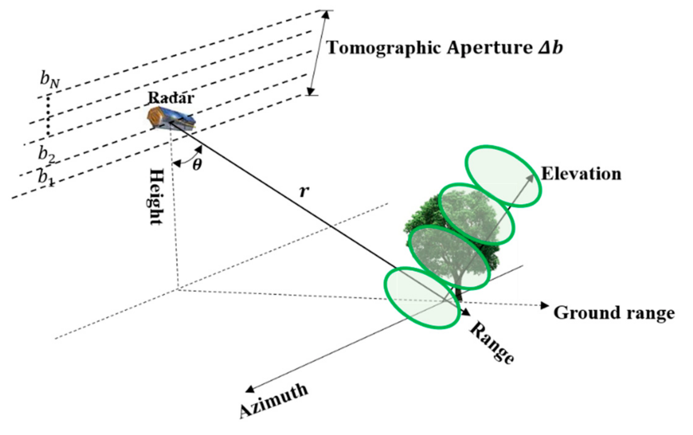
We assume that N single-look complex (SLC) SAR images are acquired over the concerned area (seen in Figure 1). Some pre-processing steps, including the selection of a common master image, co-registration, deramping, and phase calibration, are necessary to obtain the tomographic dataset. Among this dataset, the measurement in an arbitrary resolution of the nth image can be expressed as [6]:

$$y_n\left(l\right)=\int {\gamma }_z\left(l\right)\exp \left(j{k}_z\left(n\right)z\right)dz$$

(1)

where $l=1,\cdots ,L$ and L is the number of looks. $k_z\left(n\right)=\frac{4\pi b_n}{\lambda rsin\theta }$ is the vertical wavenumber between the nth image and the master image, depending on the perpendicular baseline $b_n$, the wavelength $\lambda$, the range r, and the incidence angle θ. ${\gamma }_z\left(l\right)$ indicates the vertical continuous reflectivity function, which is a complex number.

The integral of Equation (1) is discretized into the sum of backscattering reflectivity of D scatterers, which can be written as [6]:

$$y\left(l\right)=\mathit{A}x\left(l\right)+e\left(l\right)$$

(2)

where $y\left(l\right)={\left[y_1\left(l\right),y_2\left(l\right),\cdots ,y_N\left(l\right)\right]}^T$ is the observation vector composed of N images; $x\left(l\right)={[{\gamma }_{z_1}\left(l\right),\cdots ,{\gamma }_{z_D}\left(l\right)]}^T$ is the unknown discrete reflectivity vector; $z_d\left(d=1,\cdots ,D\right)$ represents the discrete position along the vertical direction; e(l) is the noise vector with N elements; and $\mathit{A}=\left[a_1,\cdots ,a_D\right]$ is an $N\times D$ coefficient matrix. The steering vector $a_d$ is given by:

$$a_d={\left[exp\left(j{k}_z\left(1\right)z_d\right),\cdots ,exp\left(j{k}_z\left(N\right)z_d\right)\right]}^T$$

(3)

where ${\left(·\right)}^T$ describes the transpose operator of a vector or a matrix.

The aim of TomoSAR is to retrieve the backscattering reflectivity power along the vertical direction, which can be regarded as a spectrum estimation problem.

2.2. The IAA Estimator

The IAA estimator is a nonparametric spectral estimation algorithm based on the WLS approach. For the TomoSAR imaging model (Equation (2)), the WLS cost function is given by [31,32,33]:

$$f={\displaystyle \sum }_{l=1}^L\Vert {y\left(l\right)-x_d\left(l\right)a_d\Vert }_{{\mathit{R}}^{-1}}^2$$

(4)

where $\mathit{R}=\mathit{A}\mathit{P}{\mathit{A}}^H$ is the covariance matrix. P is the $D\times D$ diagonal matrix of backscattering reflectivity power. ${\left(·\right)}^H$ is the conjugate transpose operator of a vector or a matrix.

The solution to minimizing Equation (4) with respect to $x_d\left(l\right)$ is given by [31,32,33]:

$$x_d\left(l\right)=\frac{a_d^H{\mathit{R}}^{-1}y\left(l\right)}{a_d^{*}{\mathit{R}}^{-1}{a}_d}$$

(5)

Thus, the corresponding power is written as [31,32]:

$$p_d=\frac{a_d^H{\mathit{R}}^{-1}\widehat{\mathit{R}}{\mathit{R}}^{-1}{a}_d}{{\left(a_d^H{\mathit{R}}^{-1}{a}_d\right)}^2}$$

(6)

where $\widehat{\mathit{R}}$ is the sample covariance matrix with $\widehat{\mathit{R}}=\frac{1}{L}{{\displaystyle \sum }}_{l=1}^L\mathrm{y}\left(l\right)\mathrm{y}{\left(l\right)}^H$.

By inspecting the above equations, parameter $x_d\left(l\right)$ and R depend on each other. Thus, an iterative solution must be adopted, as shown in

Table 1. Main steps of the IAA method.

Initialization
	$p_d=\frac{1}{{\left(a_d^H{a}_d\right)}^{2}L}{\displaystyle {\displaystyle \sum }_{l=1}^L}{\left|a_d^{H}y\left(l\right)\right|}^2 \left(d=1,\cdots ,D\right)$
Iteration
	repeat
	$\mathit{R}=\mathit{A}\mathit{P}{\mathit{A}}^H$
	$x_d\left(l\right)=\frac{a_d^H{\mathit{R}}^{-1}y\left(l\right)}{a_d^H{\mathit{R}}^{-1}{a}_d}$
	$p_d=\frac{a_d^H{\mathit{R}}^{-1}\widehat{\mathit{R}}{\mathit{R}}^{-1}{a}_d}{{\left(a_d^H{\mathit{R}}^{-1}{a}_d\right)}^2}$
	Until(convergence)

. The iterative process is terminated when the current estimates of P for the last two iterations are almost constant.

2.3. The RIAA Estimator

When the tomographic aperture is small, the vertical wavenumbers are very close to each other. This leads to the condition number of coefficient matrix A being slightly large. Accordingly, the condition number of the covariance matrix is very large, resulting in an ill-posed problem for the inversion of the covariance matrix. This easily leads to inaccurate or even wrong parameter estimations. As a result, the IAA algorithm shows a degraded performance. To overcome this problem, this paper takes into account the noise contribution to the covariance matrix within the framework of the existing IAA algorithm.

We let $\mathit{O}$ be a $\left(D+N\right)\times \left(D+N\right)$ diagonal matrix whose diagonal contains D scattering reflectivity powers of interest and N noise powers [34,35], and it can be expressed by the following:

$$\mathit{O}=\left[\begin{array}{cc}\mathit{P}& 0\\ 0& \Sigma \end{array}\right]=\left[\begin{array}{ccccccc}{p}_1& 0& \cdots & \cdots & \cdots & \cdots & 0\\ 0& p_2& 0& \cdots & \cdots & \cdots & 0\\ ⋮& 0& \ddots & ⋮& ⋮& ⋮& ⋮\\ 0& \cdots & \cdots & p_D& \cdots & \cdots & 0\\ 0& \cdots & \cdots & \cdots & {\sigma }_1^2& \cdots & 0\\ ⋮& ⋮& ⋮& ⋮& ⋮& \ddots & ⋮\\ 0& \cdots & \cdots & \cdots & \cdots & \cdots & {\sigma }_N^2\end{array}\right]$$

(7)

where the matrix P is the power matrix of the interested signal, which is the same as the power matrix in the IAA algorithm. $\mathit{\Sigma }$ is the noise power matrix, as follows:

$$\mathit{\Sigma }=\left[\begin{array}{ccc}{\sigma }_1^2& \cdots & 0\\ ⋮& \ddots & ⋮\\ 0& \cdots & {\sigma }_N^2\end{array}\right]$$

(8)

According to Equation (2), the covariance matrix R can be expressed by [34,35]:

$$\mathit{R}=\mathit{A}\mathit{O}{\mathit{A}}^H=\mathit{A}\mathit{P}{\mathit{A}}^H+\mathit{\Sigma }$$

(9)

From Equation (9), we see that $\mathit{A}\mathit{P}{\mathit{A}}^H$ is the expression of covariance matrix R in the IAA algorithm. When the tomographic aperture is small, the difference among the vertical wave numbers is small, resulting in a large condition of the mapping matrix A. Accordingly, the condition of the covariance matrix R is large, which leads to the ill-posed problem. This is sensitive to noise and is very likely to obtain a wrong estimation. When the noise covariance matrix $\Sigma$ is taken into consideration, the regularization is carried out on the diagonal elements of the matrix $\mathit{A}\mathit{P}{\mathit{A}}^H$, which overcomes the ill-posed problem. Thus, RIAA can improve the robustness of the original IAA algorithm.

From the above analysis, the solution for the covariance matrix estimation can be divided into two steps: (1) estimate the covariance matrix of the interested signal; (2) estimate the noise covariance matrix $\mathit{\Sigma }$.

For the first step, it is the same as the expression in the IAA algorithm, that is:

$$p_d=\frac{a_d^H{\mathit{R}}^{-1}\widehat{\mathit{R}}{\mathit{R}}^{-1}{a}_d}{{\left(a_d^H{\mathit{R}}^{-1}{a}_d\right)}^2}$$

(10)

For the second step, we can regard the noise as the parameter of interest. The imaging model can be rewritten as:

$$y\left(l\right)=\mathit{V}e\left(l\right)+t$$

(11)

where V is a $N\times N$ unit matrix and $t=\mathit{A}x\left(l\right)$.

According to the description in Section 2.2, the unknown parameter ${\sigma }_n^2$ can be estimated by:

$${\sigma }_n^2=\frac{v_n^H{\mathit{R}}^{-1}\widehat{\mathit{R}}{\mathit{R}}^{-1}{v}_n}{{\left(v_n^H{\mathit{R}}^{-1}{v}_n\right)}^2}$$

(12)

From Equations (9), (10) and (12), RIAA can also need an iterative process, as shown in

Table 2. Details of the RIAA estimator.

Initialization
	$$\begin{gathered} p_d=\frac{1}{{\left(a_d^H{a}_d\right)}^{2}L}{\displaystyle {\displaystyle \sum }_{l=1}^L}{\left|a_d^{H}y\left(l\right)\right|}^2 \left(d=1,\cdots ,D\right) \\ \hspace{1em}\hspace{1em}\hspace{1em}\hspace{1em}\hspace{1em}\mathit{R}\left(0\right)=\mathit{A}\mathit{P}{\mathit{A}}^H \end{gathered}$$
Iteration
	repeat
	${\sigma }_n^2=\frac{v_n^H{\mathit{R}}^{-1}\widehat{\mathit{R}}{\mathit{R}}^{-1}{v}_n}{{\left(v_n^H{\mathit{R}}^{-1}{v}_n\right)}^2}$ $\mathsf{\Sigma }=diag{\left\{{\sigma }_n^2\right\}}_{n=1}^N$ $\mathit{R}=\mathit{A}\mathit{P}{\mathit{A}}^H+\Sigma$
	4. $x_d\left(l\right)=\frac{a_d^H{\mathit{R}}^{-1}y\left(l\right)}{a_d^H{\mathit{R}}^{-1}{a}_d}$
	5. $p_d=\frac{a_d^H{\mathit{R}}^{-1}\widehat{\mathit{R}}{\mathit{R}}^{-1}{a}_d}{{\left(a_d^H{\mathit{R}}^{-1}{a}_d\right)}^2}$ 6. $\mathit{P}=diag{\left\{p_d\right\}}_{d=1}^D$
	Until(convergence)

. Moreover, the “convergence” in both Table 1 and Table 2 is $\Vert {\mathit{P}}^{current}-{\mathit{P}}^{previous}\Vert /\Vert {\mathit{P}}^{previous}\Vert \le {10}^{-4}$. This indicates that when the current estimates of P for the last two iterations remain almost constant, the iteration process is terminated.

3. Numerical Simulated Experiments

In order to investigate the superiority of the RIAA approach, the simulated parameters were set on the basis of the acquisition parameters of the E-SAR airborne system described in Tables 4 and 5.

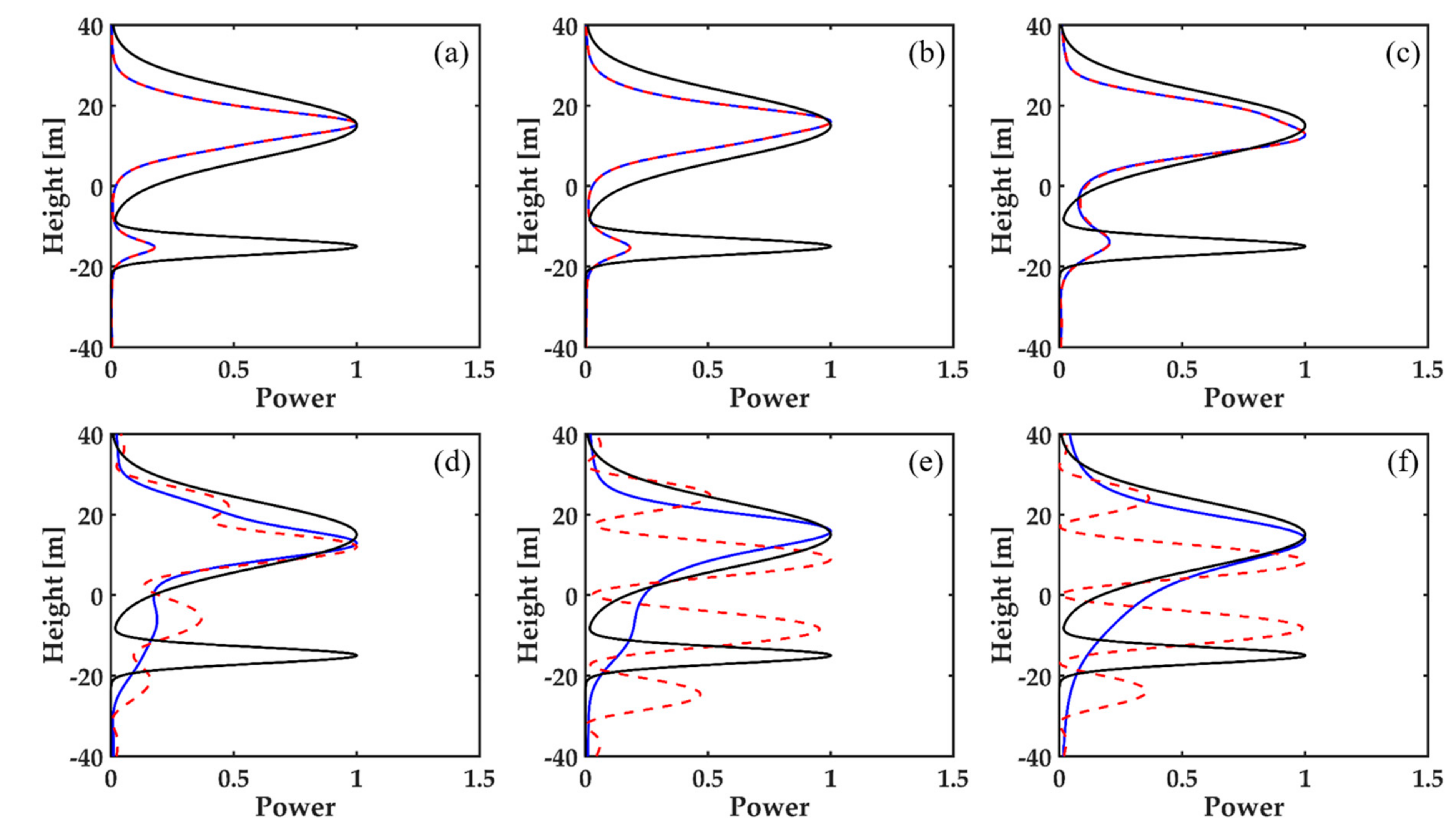
It is known that the backscattered signal in forest areas can be regarded as a two-component structure. One part represents the canopy scattering contribution, which has a higher location and a wider angular spread, and the other part represents the ground scattering contribution [13,30,32]. Thus, we simulated the backscattered signal with a canopy phase center of 15 m and a ground phase center of −15 m. Moreover, the signal-to-noise ratio was 20 dB. Three kinds of forest scattering scenarios were simulated as follows: (1) the ground scattering contribution dominates; (2) the ground scattering contribution is the same as the canopy scattering contribution; (3) the canopy scattering contribution dominates. After that, based on the well-known TomoSAR imaging model (as shown in Equation (2)), the observation vector was simulated. Both the IAA and RIAA estimators were carried out to obtain the reflectivity profile with different tomographic apertures (30 m, 25 m, 20 m, 15 m, 10 m, and 5 m) in these three simulated scattering scenarios, as shown in Figure 2, Figure 3 and Figure 4.

Some observations can be made from the above simulations, as follows:

(1)

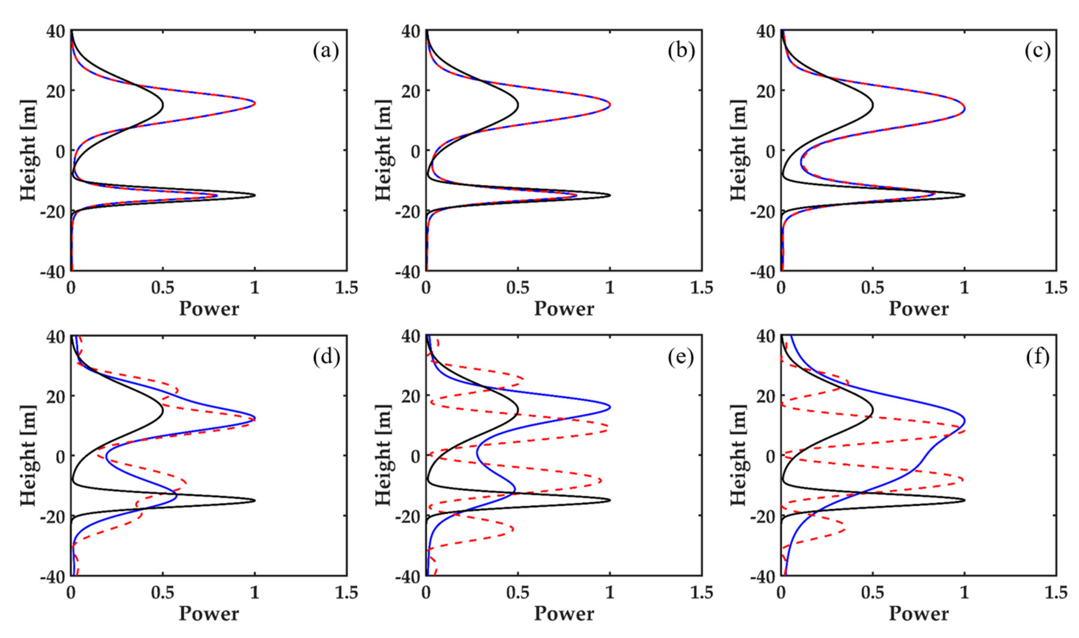
In the case of the ground contribution dominating, both the IAA and RIAA algorithms successfully reconstruct the forest canopy and ground scattering contribution with the large tomographic aperture (i.e., 30 m, 25 m, and 20 m). However, when the synthetic aperture is reduced to 15 m, 10 m and 5 m, the IAA algorithm detects the canopy and the ground scattering contribution with a large deviation. Although the RIAA algorithm has some error in detecting the ground scattering center, it can still successfully recover the ground and canopy scattering contribution.

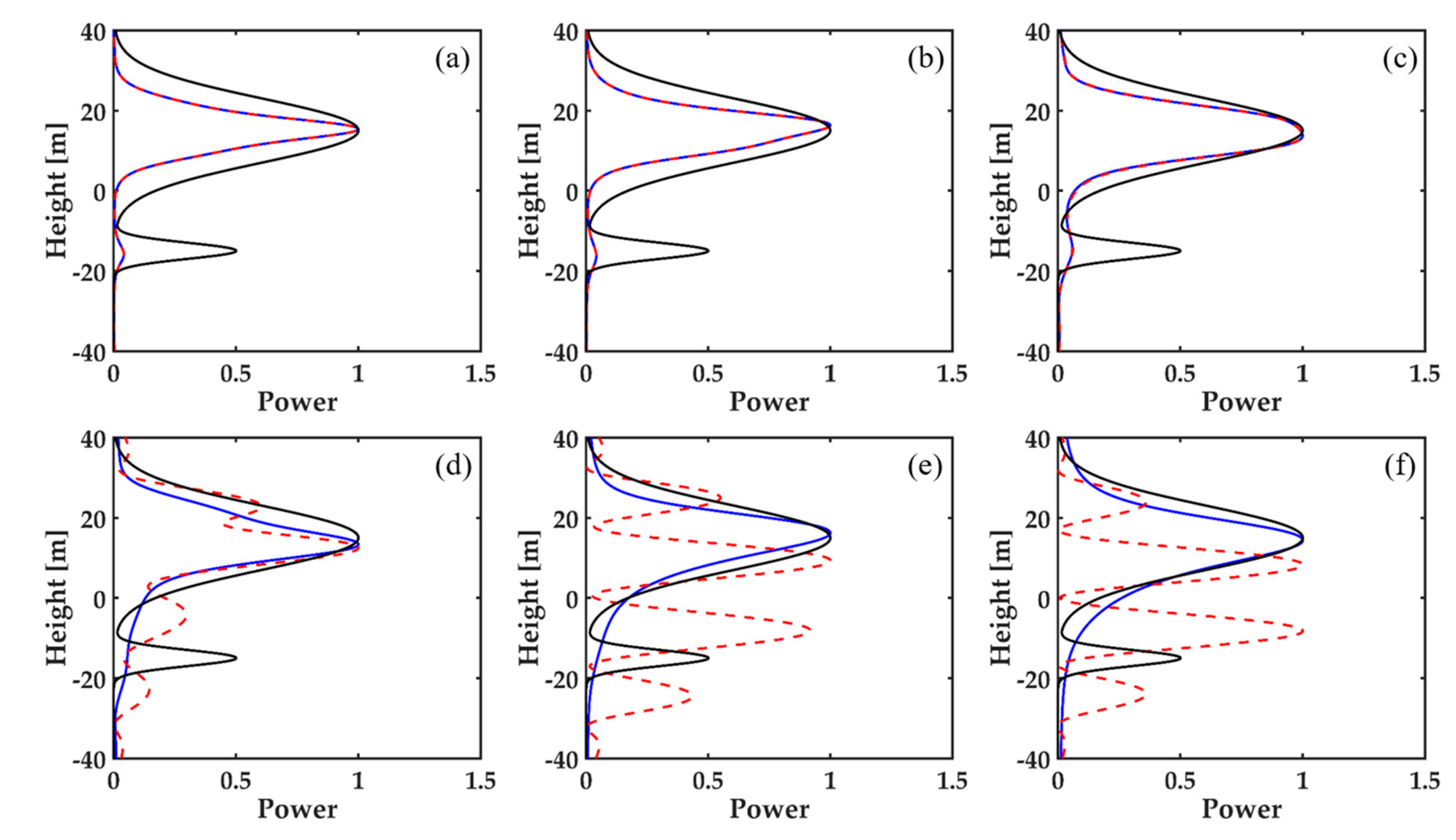
(2)

When the ground scattering contribution is the same as the canopy scattering contribution, IAA and RIAA have the same performance in the case of the large tomographic aperture (i.e., 30 m, 25 m, and 20 m). They can successfully discriminate the canopy and ground scattering contribution while having a reduced ability to detect the ground scattering contribution. When the tomographic aperture becomes small (i.e., 15 m, 10 m, and 5 m), the IAA algorithm has a large misestimation result, while the RIAA algorithm can still accurately estimate the ground and canopy scattering contribution.

(3)

When the canopy contribution dominates, in the case of the large tomographic aperture (i.e., 30 m, 25 m, and 20 m), both the IAA algorithm and the RIAA algorithm can successfully obtain the forest canopy scattering contribution, but they have a weak ability to detect the surface scattering. However, when the synthetic aperture is reduced to 15 m, 10 m and 5 m, the IAA algorithm cannot accurately estimate the canopy and ground scattering contribution. The RIAA algorithm cannot detect the ground scattering contribution, but it can accurately recover the canopy scattering contribution.

In summary, for these three simulated forest scattering scenarios, the RIAA algorithm has the same performance as the IAA algorithm in the case of a large tomographic aperture (i.e., 30 m, 25 m, and 20 m), but it has a much better performance than the IAA estimator in the case of a small tomographic aperture (i.e., 15 m, 10 m, and 5 m). Accordingly, we calculated the condition number of the covariance matrix with different tomographic apertures, as listed in

Table 3. Condition number of the covariance matrix with different tomographic apertures.

Tomographic Aperture Length	Condition Number
30	6.80
25	14.68
20	142.27
15	5493.20
10	1.83 × 105
5	3.72 × 108

. It is found that the condition number of the covariance matrix becomes larger as the tomographic aperture becomes smaller. For a large condition number, it causes the ill-posed problem for the inversion of the covariance matrix, which can be solved by considering the noise contribution to the covariance matrix estimation. This can be regarded as a regularization on the diagonal elements of the covariance matrix. Thus, IAA shows a degraded performance, while RIAA can still perform well in the case of a small tomographic aperture.

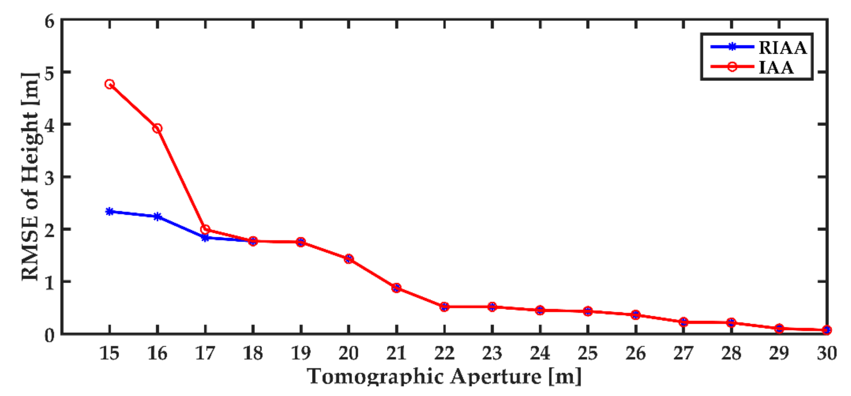
Moreover, for exploring the tomographic aperture at which the RIAA and IAA methods begin to diverge, the root-mean-square-errors (RMSEs) of scattering phase center height estimated by these two approaches were calculated with different tomographic apertures, as shown in Figure 5. It is clear that the two estimators start to diverge at the tomographic aperture of around 17m in this case. With the decrease in the tomographic aperture, RIAA shows a better performance than IAA. This suggests that RIAA is a more robust TomoSAR method in the case of a small tomographic aperture.

4. Real-Data Experiments and Results

To further investigate the feasibility and effectiveness of the RIAA TomoSAR method, a set of real airborne SAR images was used to estimate the forest height.

4.1. Study Area and Dataset

The study area is the boreal forests in the Krycklan Catchment, North Sweden, including coniferous forests such as scotch pine and Norway spruce, and a few birch trees. The average annual temperature here is about 1 °C and the average annual precipitation is 600 mm. Moreover, the terrain topography is hilly with varying from 190 m to 290 m. The average tree height is about 18m and the maximum tree height is 30 m [36].

A set of six L-band SAR images in fully polarimetric mode over the study area was acquired by the German Aerospace Centre (DLR) in the framework of the ESA BioSAR 2008 campaign on 15 October 2008. The BioSAR2008 project was carried out by the cooperation of the European Space Agency (ESA), the German Aerospace Centre (DLR), the Swedish Defense Research Agency (FOI), the Swedish University of Agricultural Sciences (SLU), the Biosphere Remote Sensing Research and Education Centre (CESBIO) and the Polytechnic of Milan, Italy, which aimed at addressing some important specific requirements of ESA’s earth resources exploration program BIOMASS [36]. This dataset has performed some necessary pre-processing steps, such as co-registration and flat-earth phase removal. The range resolution is 2.12 m and the azimuth resolution is 1.20 m. The incidence angle ranges from 25° to 55° from the near range to the far range. The tomographic aperture varies from 30 m at the near range to 7.2 m at the far range [36]. Additionally, the height resolution varies from 6m in the near range to 25 m in the far range.

Table 4. The parameters of the E-SAR airborne system.

Wavelength Polarimetric Channel	0.23 m (L-Band) HH + HV + VV
Incidence angle	25°–55°
Center slant range	3900 m
Range resolution	2.12 m
Azimuth resolution	1.20 m

and

Table 5. The baseline information for the InSAR pairs.

Identifier	Acquisition Date	Baseline (m)
08biosar0201×1	15/10/2008	0
08biosar0203×1		−6
08biosar0205×1		−12
08biosar0207×1		−18
08biosar0209×1		−24
08biosar0211×1		−30

, respectively, present details of the parameters of the E-SAR airborne system and the baseline information for the interferometric synthetic aperture radar (InSAR) pairs.

In addition, in order to validate the result of the SAR tomography, this project carried a helicopter laser radar S/N425 TopEye system on the platform to generate a series of point cloud data over this study area on 5 August and 6 August 2008. From these point cloud data, the canopy height model (CHM) was obtained.

4.2. Results and Analysis

4.2.1. Tomograms of the Selected Azimuth Profiles

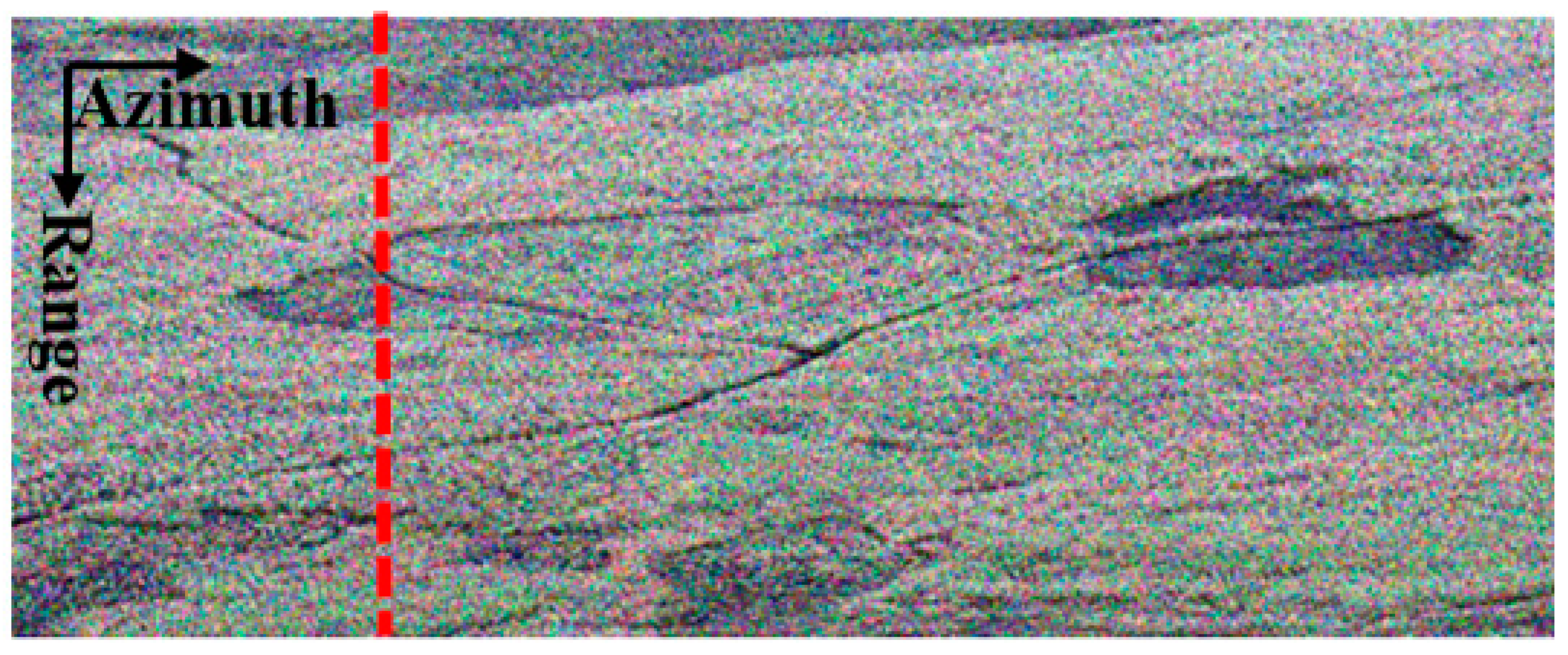
A range profile (the red dotted line, as shown in Figure 6) was selected as an example for tomographic focusing. This profile was fixed at the 500th azimuth resolution cell.

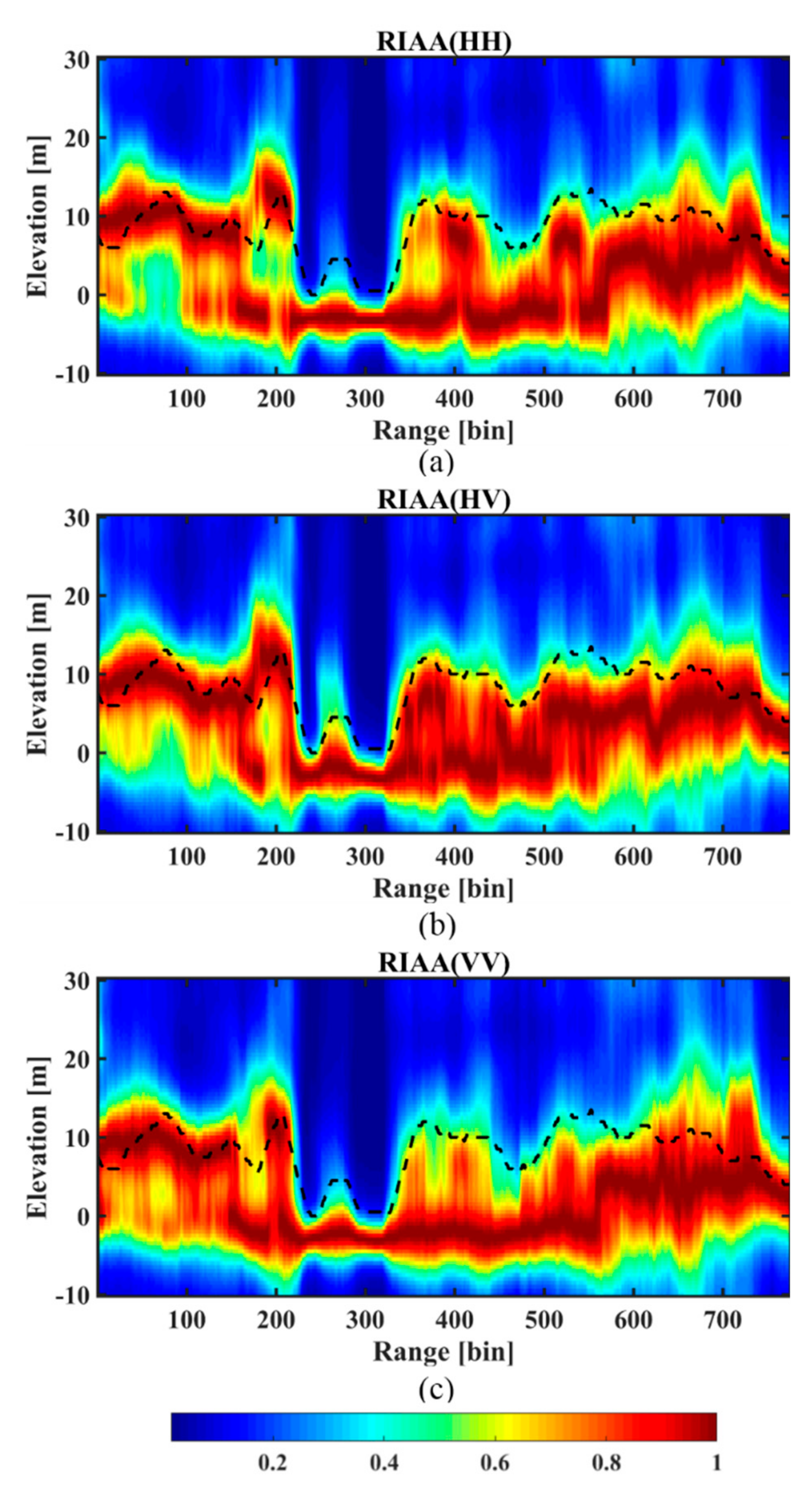
Figure 7 represents the tomograms of the three polarimetric channels for the selected range profile. In order to directly relate the vertical coordinates to the elevation of the targets above ground, an operation to flatten the topography was carried out. Meanwhile, the corresponding CHM was superimposed on the map, for the sake of comparison. We can find that the RIAA method can successfully retrieve the forest vertical structure in three polarizations. Moreover, the canopy scattering phase center heights are consistent with the LiDAR CHM measurements. The scattering phase centers of the HV channel are more concentrated in the canopy than those from HH and VV channels. However, the tomograms from three polarimetric channels are basically similar. This is because it is a boreal forest where the forest height is not high and the canopy is not dense. The L-band can penetrate the forest and reach the ground. This is consistent with the research findings in the literature [13].

4.2.2. Forest Height Estimation

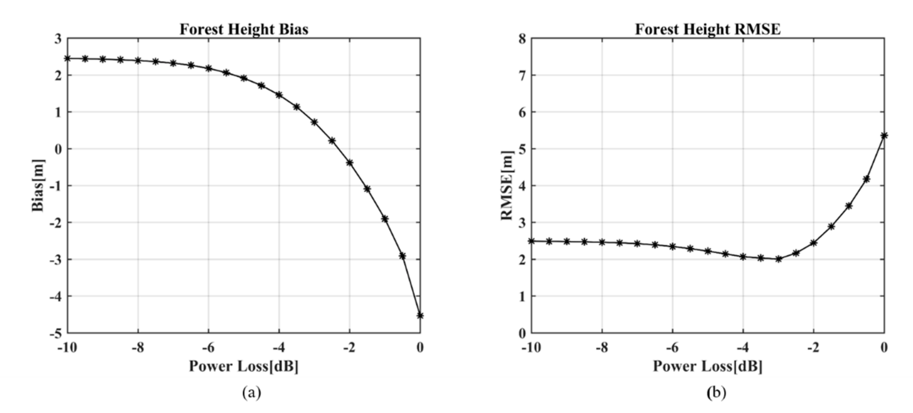
From the analysis in Section 4.2.1, the forest height can be obtained from the results of the HV channel. However, it is clear that the peak position of the tomogram is the phase center height of the forest volume scattering, rather than the tree top height. According to the research described in [13,30,32], the forest height can be determined by evaluating the power loss from the phase center location. Therefore, we should determine the power loss from the phase center at first.

The power loss location could be extracted with the help of the LiDAR CHM [13,30,32]. We estimated the forest height under different power losses ranging from −10 dB to 0 dB, and we calculated the difference between the calculated forest height and the LiDAR CHM. Figure 8 shows the bias and the RMSE of the forest height estimated by the RIAA TomoSAR estimator under different power losses with respect to the LiDAR CHM measurements. At a power loss of about 3 dB, the RMSE is the minimum and the bias is also small. Thus, the location of 3 dB power loss is determined as the forest height location of the RIAA TomoSAR estimator. When the LiDAR data are unavailable, the tree height information of several sample plots should be measured in situ to estimate the power loss location.

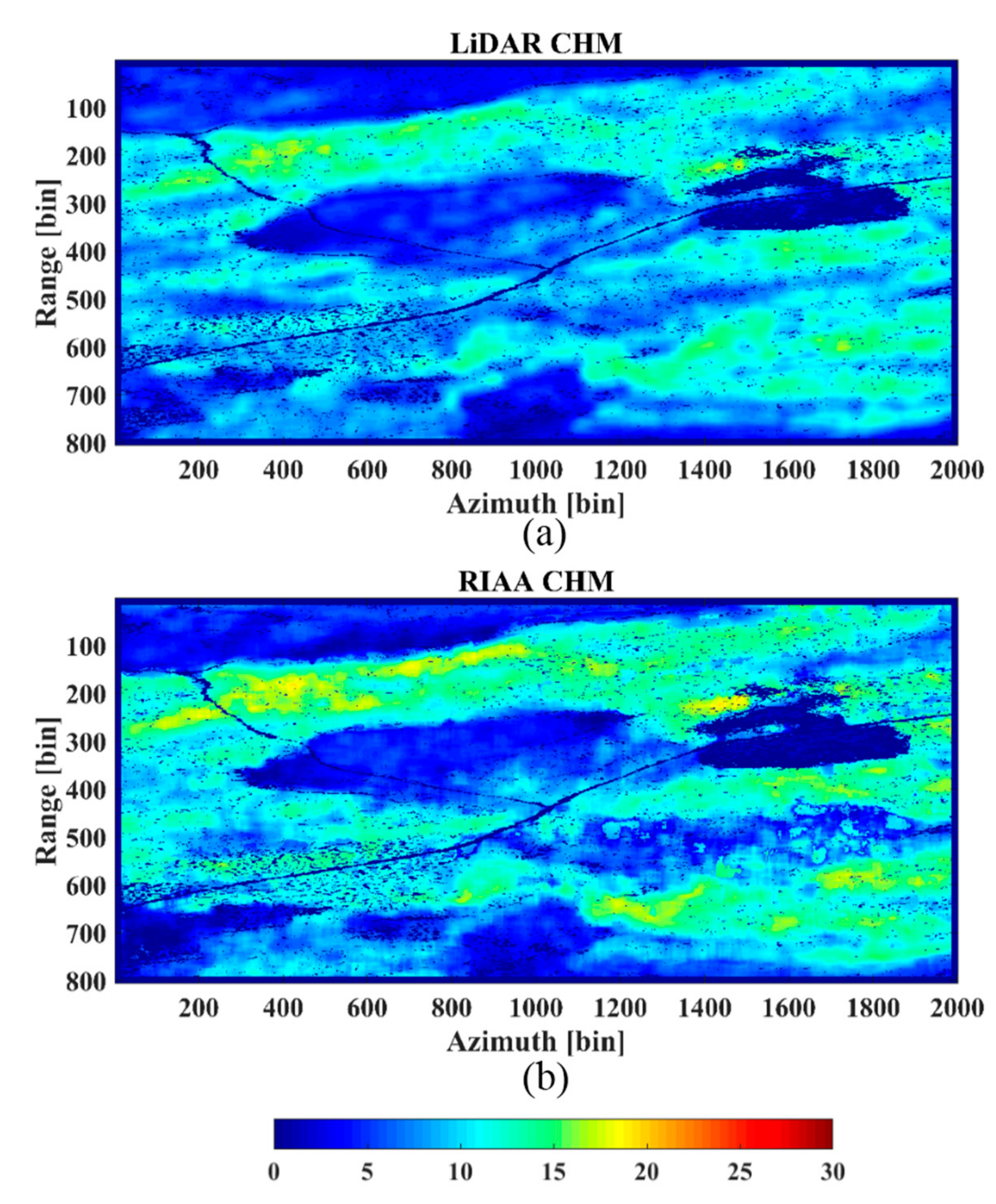
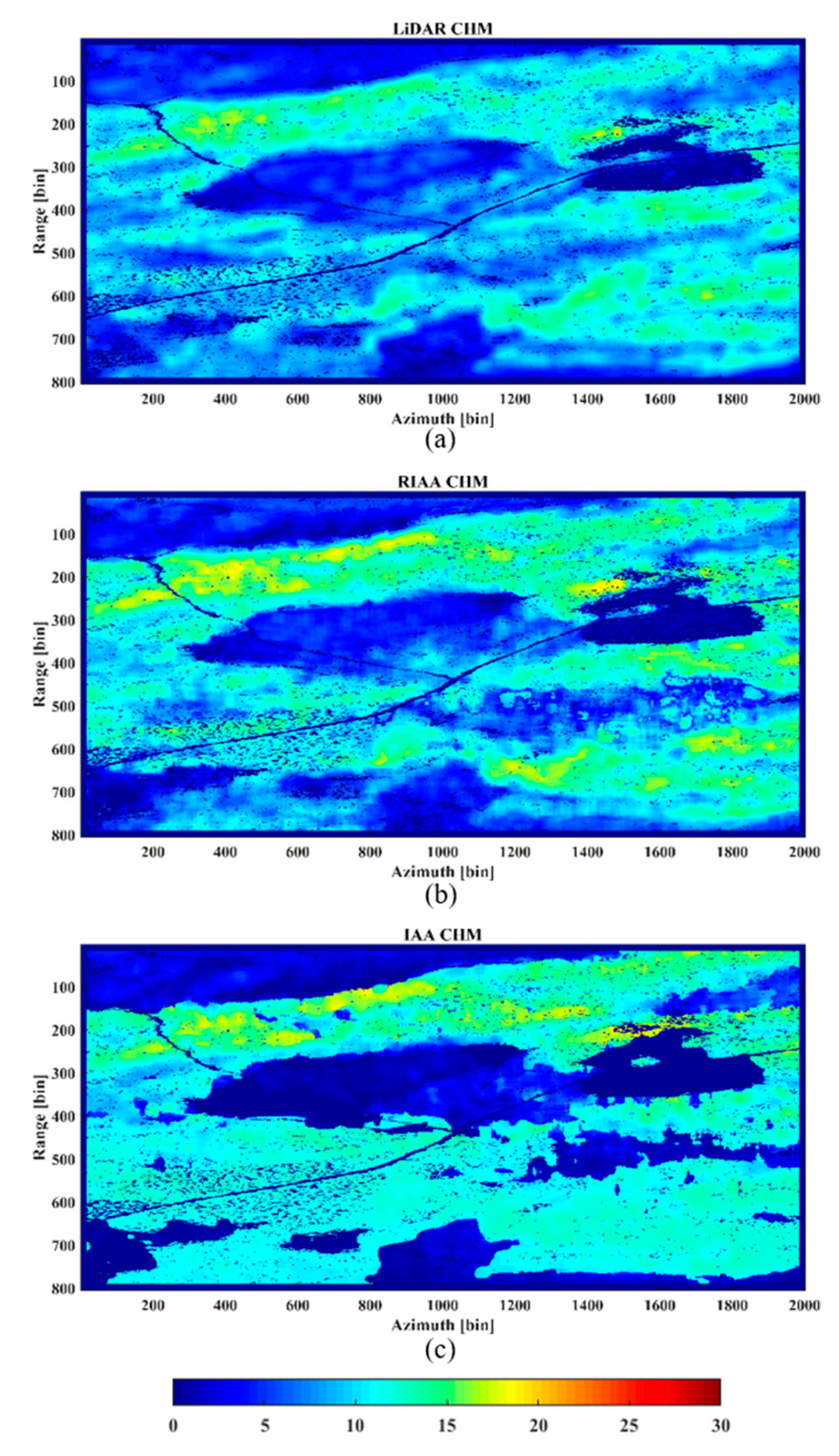
The LiDAR CHM and the forest height estimated by the RIAA estimator are shown in Figure 9. It can be seen that the forest height estimation of the RIAA TomoSAR method varies from about 0 m to 30 m, which keeps in conformity with the truth over this study area. However, some bias does occur because of the influence of several factors, such as the estimation error.

Moreover, we calculated the mean and RMSE of the forest height estimated by the RIAA TomoSAR method relative to the LiDAR CHM, as listed in

Table 6. Mean and RMSE of the forest height estimated by RIAA with respect to the LiDAR CHM.

TomoSAR w.r.t LiDAR	Mean	RMSE
Forest height (m)	0.72	2.01

. The mean and RMSE are, respectively, 0.72 m and 2.01 m. This suggests that the forest height estimated by the RIAA algorithm is reliable.

5. Discussion

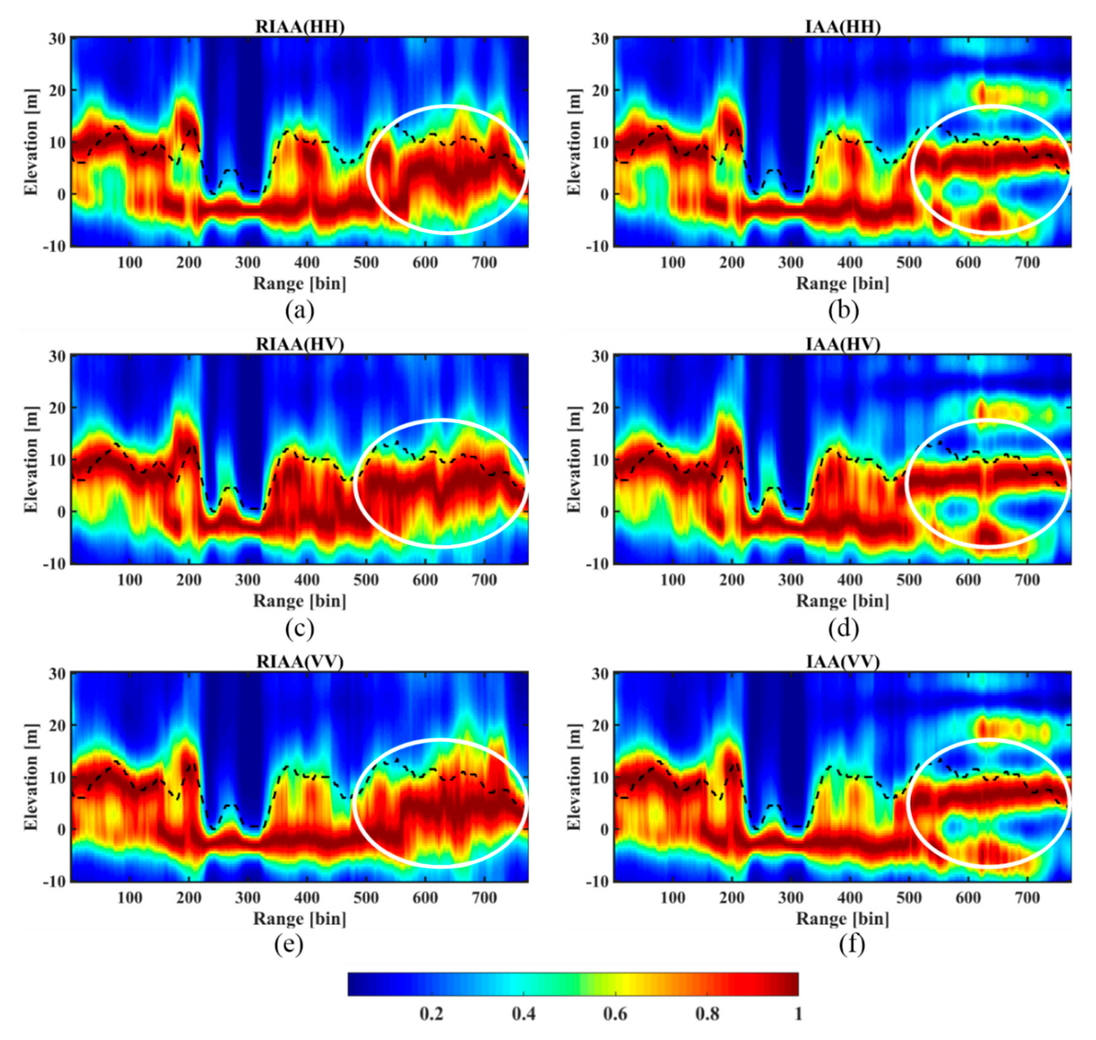
In order to further demonstrate the advantage of the RIAA TomoSAR method, IAA was also used to undertake tomographic focusing at the same range profile. The same parameters (estimation window, height range, and height sample interval) were used in the IAA method. Figure 10 shows the reconstructed tomograms in three polarizations from RIAA and IAA estimators, respectively.

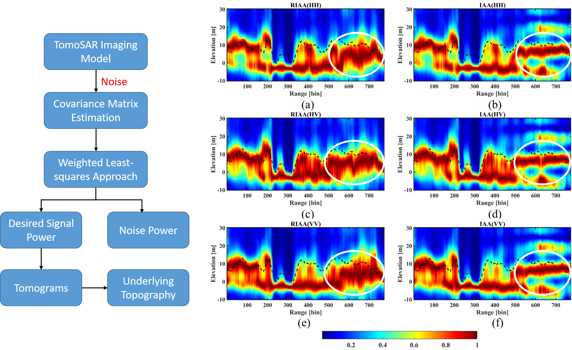
It can be seen that there are different performances at the near and far range. For the near-range segment (from the 1st to 500th range bin), the RIAA and IAA estimators show the same performance in three polarizations, and their results are consistent with the LiDAR CHM measurements. However, for the far-range part (from the 501st range bin to the end), it is clear that the RIAA estimator obtains better results than the IAA estimator in three polarizations. (1) The tomogram estimated by the RIAA estimator is as good as the near-range tomogram, agreeing well with the CHM measurements, whereas the IAA estimator shows a seriously degraded result which hardly reflects the vertical structure of the forest, especially the parts marked by the white circles. (2) There are no sidelobes in the result of the RIAA estimator, while two sidelobes are, respectively, located at about 20 m and −10 m for the tomogram of the IAA estimator.

Furthermore, the forest height was also obtained by the IAA estimator, as shown in Figure 11c. For the sake of comparison, we divided the study area into two parts: the near-range part (the area from the 1st to the 500th range bin) and the far-range part (the remaining area). For the near-range part, the forest height estimations of the two methods are very similar, and they are both similar to the LiDAR CHM. However, for the far-range part, the estimation of the RIAA estimator is clearly closer to the LiDAR CHM than that of the IAA estimator. This is because the RIAA estimator can successfully reconstruct the forest vertical profiles from the near range to the far range, but the IAA estimator shows a degraded performance in the far range (as shown in Section 4.2.2).

Moreover, we calculated the RMSE of the forest height estimated by the IAA TomoSAR estimator with respect to the LiDAR CHM, as listed in

Table 7. RMSEs of the forest height estimated by RIAA and IAA with respect to the LiDAR CHM.

TomoSAR w.r.t LiDAR	RIAA	IAA
RMSE (m)	2.01	3.25

. The RMSE is 2.01 m for the RIAA TomoSAR estimator and 3.25 m for the IAA TomoSAR estimator. This suggests that the forest height estimation accuracy of the RIAA estimator is higher than that of the IAA estimator.

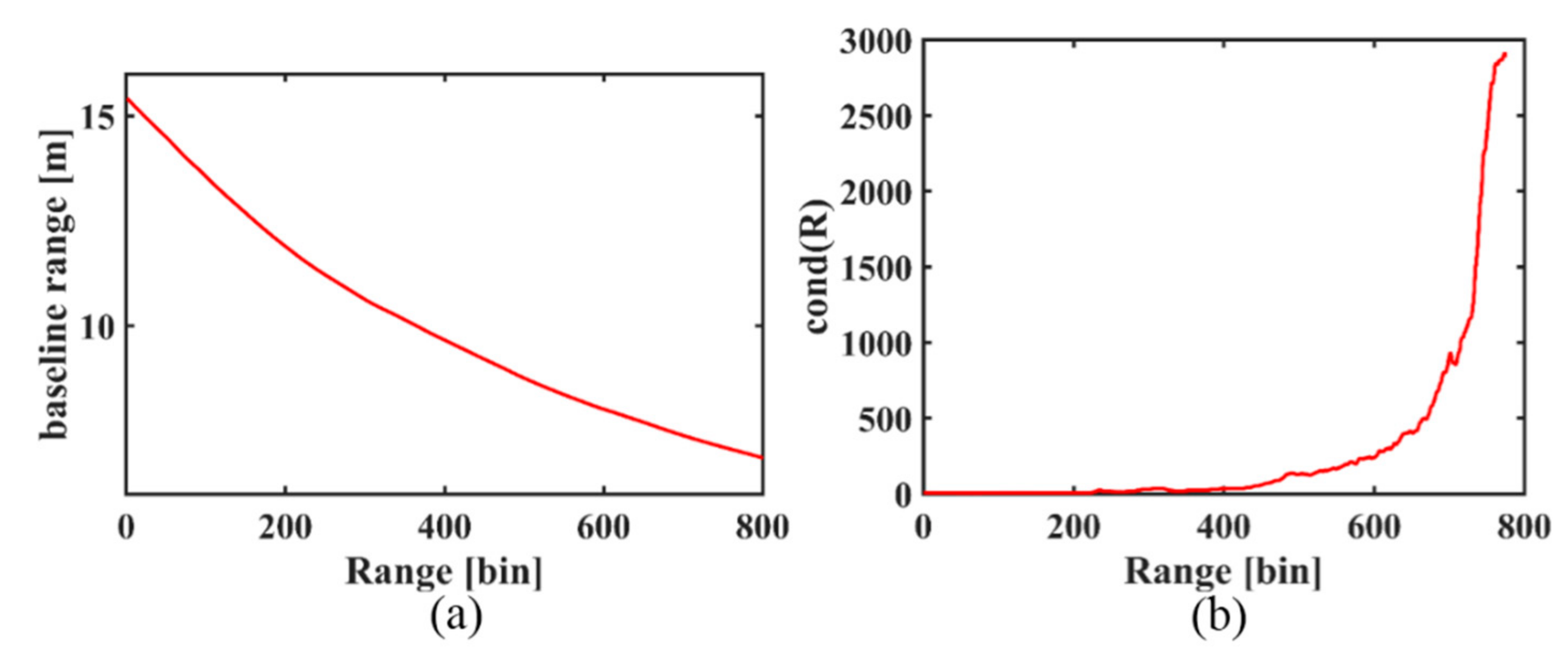
In addition, to analyze the different performances of IAA and RIAA between the near range and far range, the condition number of the covariance matrix was calculated at different range locations (see Figure 12). This indicates that the tomographic aperture decreases and the condition number of the covariance matrix increases from the near range to the far range, especially after the 500th range bin. This brings about the ill-posed problem for the inversion of the covariance matrix for the IAA estimator in the far-range part. However, by considering the noise contribution, RIAA can ensure that the condition number of the covariance matrix is not too large. Thus, in this case study, RIAA can always achieve a pleasing performance, from the near range to the far range, whereas IAA cannot achieve this.

6. Conclusions

In this paper, we have proposed a robust nonparametric iterative adaptive approach (RIAA) for TomoSAR in the case of a small tomographic aperture. The RIAA algorithm extends the existing IAA-based methodology by considering the additive noise term in the covariance matrix estimation, which avoids the ill-posed problem and improves the robustness of the IAA estimator. When the tomographic aperture is large, the RIAA and IAA estimators show the same performance. When the tomographic aperture is small, RIAA shows a better performance than IAA.

In this case study, a set of simulated experiments was carried out, and the results confirmed the superiority of the RIAA estimator in the case of a small tomographic aperture for three simulated forest scattering scenarios. The RIAA and IAA tomographic estimators were applied to the BioSAR 2008 fully polarimetric L-band airborne SAR dataset from the Krycklan Catchment, Northern Sweden. The results showed that the RIAA estimator can always obtain an accurate vertical structure for the forest, from the near range to the far range, whereas the IAA estimator works poorly in the far range, with serious sidelobes and wrong estimations. Moreover, the forest height was obtained by both the RIAA and IAA TomoSAR estimators. With respect to the LiDAR data, the RMSE of the estimations from the RIAA TomoSAR estimator was 2.01 m, which is better than that of the IAA estimator with 3.25 m. This suggests that the RIAA estimator can obtain more reliable results than the IAA estimator for application in forest areas. The reason for this is that, in the far-range area, the tomographic aperture is small and the condition number of the covariance matrix is large. In conclusion, the RIAA method has the advantages of a higher resolution and higher estimation accuracy than the IAA approach in the case of a small tomographic aperture.

Our future work will focus on analyzing the robustness of the proposed approach with fully polarimetric tomographic SAR datasets and the application of differential TomoSAR.

References

- Simard, M.; Pinto, N.; Fisher, J.B.; Baccini, A. Mapping forest canopy height globally with spaceborne lidar. J. Geophys. Res. 2011, 116. [Google Scholar] [CrossRef] [Green Version]
- Le Toan, T.; Quegan, S.; Davidson, M.W.J.; Balzter, H.; Paillou, P.; Papathanassiou, K.; Plummer, S.; Rocca, F.; Saatchi, S.; Shugart, H.; et al. The BIOMASS mission: Mapping global forest biomass to better understand the terrestrial carbon cycle. Remote Sens. Environ. 2011, 115, 2850–2860. [Google Scholar] [CrossRef] [Green Version]
- Kugler, F.; Schulze, D.; Hajnsek, I.; Papathanassiou, K.P. TanDEM-X Pol-InSAR performance for forest height estimation. IEEE Trans. Geosci. Remote Sens. 2014, 52, 6404–6422. [Google Scholar] [CrossRef]
- Kumar, S.; Khati, U.G.; Chandola, S.; Agrawal, S.; Kushwaha, S.P. Polarimetric SAR Interferometry based Modeling for Tree Height and Aboveground Biomass Retrieval in a Tropical Deciduous Forest. Adv. Space Res. 2017, 60, 571–586. [Google Scholar] [CrossRef]
- Fu, H.Q.; Wang, C.C.; Zhu, J.J.; Xie, Q.; Zhang, B. Estimation of pine forest height and underlying DEM using multi-baseline P-band PolInSAR data. Remote Sens. 2016, 8, 820. [Google Scholar] [CrossRef] [Green Version]
- Reigber, A.; Moreira, A. First Demonstration of Airborne SAR Tomography Using Multibaseline L-band Data. IEEE Trans. Geosci. Remote Sens. 2000, 38, 2142–2152. [Google Scholar] [CrossRef]
- Ho Tong Minh, D.; Ngo, Y.N.; Lê, T.T. Potential of P-Band SAR Tomography in Forest Type Classification. Remote Sens. 2021, 13, 696. [Google Scholar] [CrossRef]
- Aghababaei, H.; Ferraioli, G.; Ferro-Famil, L.; Huang, Y.; d’Alessandro, M.M.; Pascazio, V.; Schirinzi, G.; Tebaldini, S. Forest SAR tomography: Principles and applications. IEEE Geosci. Remote Sens. Mag. 2020, 8, 30–45. [Google Scholar] [CrossRef]
- Tebaldini, S.; Minh, D.H.T.; d’Alessandro, M.M.; Villard, L.; Le Toan, T.; Chave, J. The status of technologies to measure forest biomass and structural properties: State of the art in SAR tomography of tropical forests. Surv. Geophys. 2019, 40, 779–801. [Google Scholar] [CrossRef]
- Blomberg, E.; Ferro-Famil, L.; Soja, M.J.; Ulander, L.M.; Tebaldini, S. Forest biomass retrieval from L-band SAR using tomographic ground backscatter removal. IEEE Geosci. Remote Sens. Lett. 2018, 15, 1030–1034. [Google Scholar] [CrossRef]
- Aghababaee, H.; Ferraioli, G.; Schirinzi, G.; Sahebi, M.R. The role of nonlocal estimation in SAR tomographic imaging of volumetric media. IEEE Geosci. Remote Sens. Lett. 2018, 15, 729–733. [Google Scholar] [CrossRef]
- Tello, M.; CazcarraBes, V.; Pardini, M.; Papathanassiou, K. Assessment of forest structure estimation by means of SAR tomography: Potential and limitations. In Proceedings of the IEEE International Geoscience and Remote Sensing Symposium (IGARSS), Beijing, China, 10–15 July 2016; pp. 32–35. [Google Scholar]
- Tebaldini, S.; Rocca, F. Multibaseline Polarimetric SAR Tomography of a Boreal Forest at P- and L- Bands. IEEE Trans. Geosci. Remote Sens. 2012, 50, 232–246. [Google Scholar] [CrossRef]
- Minh, D.H.T.; Le Toan, T.; Rocca, F.; Tebaldini, S. SAR Tomography for the Retrieval of Forest Biomass and Height: Cross-validation at Two Tropical Forest Sites in French Guiana. Remote Sens. Environ. 2016, 175, 138–147. [Google Scholar] [CrossRef] [Green Version]
- Li, L.; Chen, E.; Li, Z.; Zhao, L.; Gu, X. Forest above ground biomass estimation from P-band tomography data. In Proceedings of the IEEE International Geoscience and Remote Sensing Symposium (IGARSS), Beijing, China, 10–15 July 2016; pp. 21–23. [Google Scholar]
- Kumar, S.; Joshi, S.K.; Govil, H. Spaceborne PolSAR Tomography for Forest Height Retrieval. IEEE J. Sel. Top. Appl. Earth Observ. Remote Sens. 2017, 10, 5175–5185. [Google Scholar] [CrossRef]
- Yu, H.; Zhang, Z. The Performance of Relative Height Metrics for Estimation of Forest Above-Ground Biomass Using L-and X-Bands TomoSAR Data. IEEE J. Sel. Top. Appl. Earth Obs. Remote Sens. 2021, 14, 1857–1871. [Google Scholar] [CrossRef]
- Gustavo, D.; del Campo, M.; Reigber, A.; Shkvarko, Y.V. Resolution enhanced SAR tomography: A Nonparametric Iterative Adaptive Approach. In Proceedings of the 2016 IEEE International Geoscience and Remote Sensing Symposium (IGARSS), Beijing, China, 10–15 July 2016; pp. 3238–3241. [Google Scholar]
- Peng, X.; Wang, C.; Li, X.; Du, Y.; Fu, H.; Yang, Z.; Xie, Q. Three-Dimensional Structure Inversion of Buildings with Nonparametric Iterative Adaptive Approach Using SAR Tomography. Remote Sens. 2018, 10, 1004. [Google Scholar] [CrossRef] [Green Version]
- Wei, L.; Balz, T.; Zhang, L.; Liao, M. A novel fast approach for SAR tomography: Two-step iterative shrinkage/thresholding. IEEE Geosci. Remote Sens. Lett. 2015, 12, 1377–1381. [Google Scholar]
- Fornaro, G.; Serafino, F.; Soldovieri, F. Three-dimensional Focusing with Multi-pass SAR Data. IEEE Trans. Geosci. Remote Sens. 2003, 41, 507–517. [Google Scholar] [CrossRef]
- Sauer, S.; Ferro-Famil, L.; Reigber, A.; Pottier, E. Three-dimensional imaging and scattering mechanism estimation over urban scenes using dual-baseline polarimetric InSAR observations at L-band. IEEE Trans. Geosci. Remote Sens. 2011, 49, 4616–4629. [Google Scholar] [CrossRef] [Green Version]
- Huang, Y.; Ferro-Famil, L.; Reigber, A. Under-foliage Object Imaging Using SAR Tomography and Polarimetric Spectral Estimators. IEEE Trans. Geosci. Remote Sens. 2012, 50, 2213–2225. [Google Scholar] [CrossRef] [Green Version]
- Huang, Y.; Zhang, Q.; Ferro-Famil, L. Forest Height Estimation Using a Single-Pass Airborne L-Band Polarimetric and Interferometric SAR System and Tomographic Techniques. Remote Sens. 2021, 13, 487. [Google Scholar] [CrossRef]
- Budillon, A.; Evangelista, A.; Schirinzi, G. Three dimensional SAR focusing from multi-pass signals using compressive sampling. IEEE Trans. Geosci. Remote Sens 2011, 40, 488–499. [Google Scholar] [CrossRef]
- Aguilera, E.; Nannini, M.; Reigbe, A. Wavelet-Based Compressed Sensing for SAR Tomography of Forested Areas. IEEE Trans. Geosci. Remote Sens. 2013, 51, 5283–5295. [Google Scholar] [CrossRef] [Green Version]
- Bi, H.; Liu, J.; Zhang, B.; Hong, W. Baseline distribution optimization and missing data completion in wavelet-based CS-TomoSAR. Sci. China Inf. Sci. 2018, 61, 042302. [Google Scholar] [CrossRef]
- El Moussawi, I.; Ho Tong Minh, D.; Baghdadi, N.; Abdallah, C.; Jomaah, J.; Strauss, O.; Lavalle, M.; Ngo, Y.N. Monitoring Tropical Forest Structure Using SAR Tomography at L-and P-Band. Remote Sens. 2019, 11, 1934. [Google Scholar] [CrossRef] [Green Version]
- Cazcarra-Bes, V.; Tello-Alonso, M.; Fischer, R.; Heym, M.; Papathanassiou, K. Monitoring of Forest Structure Dynamics by means of L-band SAR Tomography. Remote Sens. 2017, 9, 1229. [Google Scholar] [CrossRef] [Green Version]
- Li, X.W.; Liang, L.; Guo, H. Compressive Sensing for Multibaseline Polarimetric SAR Tomography of Forested Areas. IEEE Trans. Geosci. Remote Sens. 2016, 54, 153–166. [Google Scholar] [CrossRef]
- Del Campo, G.M.; Nannini, M.; Reigber, A. Statistical Regularization for Enhanced TomoSAR Imaging. IEEE J. Sel. Top. Appl. Earth Obs. Remote Sens. 2020, 13, 1567–1589. [Google Scholar] [CrossRef]
- Peng, X.; Li, X.; Wang, C.; Zhu, J.; Liang, L.; Fu, H.; Du, Y.; Yang, Z.; Xie, Q. SPICE-based SAR Tomography over Forest Areas Using a Small Number of P-band Airborne F-SAR Dataset Characterized by Non-uniformly Distributed Baselines. Remote Sens. 2019, 11, 975. [Google Scholar] [CrossRef] [Green Version]
- Yardibi, T.; Li, J.; Stoica, P.; Xue, M.; Baggeroer, A.B. Source localization and sensing: A nonparametric iterative adaptive approach based on weighted least squares. IEEE Trans. Aerosp. Electron. Syst. 2010, 46, 425–443. [Google Scholar] [CrossRef]
- Roberts, W.; Stoica, P.; Li, J.; Yardibi, T.; Sadjadi, F.A. Iterative Adaptive Approaches to MIMO Radar Imaging. IEEE J. Sel. Top. Signal Process. 2010, 4, 5–20. [Google Scholar] [CrossRef]
- Yang, Z.; Li, X.; Wang, H.; Jiang, W. Adaptive clutter suppression based on iterative adaptive approach for airborne radar. Signal Process. 2013, 93, 3567–3577. [Google Scholar] [CrossRef]
- European Space Agency. Technical Assistance for the Development of Airborne SAR and Geophysical Measurements during the BioSAR 2008 Experiment; Final Report; European Space Agency: Paris, France, 2009. [Google Scholar]
Figure 1.
The geometry of TomoSAR over forest areas.
Figure 2.
Reconstructed reflectivity profiles by the RIAA and IAA methods with different tomographic apertures in the first scattering scenario: (a) 30 m; (b) 25 m; (c) 20 m; (d) 15 m; (e) 10 m; (f) 5 m. The black solid lines are the true simulated reflectivity profiles. The blue solid lines are the reconstructed reflectivity profiles of RIAA. The red dotted lines are the reconstructed reflectivity profiles of IAA.
Figure 3.
Reconstructed reflectivity profiles by the RIAA and IAA methods with different tomographic apertures in the second scattering scenario: (a) 30 m; (b) 25 m; (c) 20 m; (d) 15 m; (e) 10 m; (f) 5 m. The black solid lines are the true simulated reflectivity profiles. The blue solid lines are the reconstructed reflectivity profiles of RIAA. The red dotted lines are the reconstructed reflectivity profiles of IAA.
Figure 4.
Reconstructed reflectivity profiles by the RIAA and IAA methods with different tomographic apertures in the third scattering scenario: (a) 30 m; (b) 25 m; (c) 20 m; (d) 15 m; (e) 10 m; (f) 5 m. The black solid lines are the true simulated reflectivity profiles. The blue solid lines are the reconstructed reflectivity profiles of RIAA. The red dotted lines are the reconstructed reflectivity profiles of IAA.
Figure 5.
RMSEs of scattering phase center height estimated by RIAA and IAA methods with different tomographic apertures.
Figure 6.
The selected azimuth profile (red dotted line) on the SAR intensity map.
Figure 7.
The tomograms of the selected profile estimated by the RIAA method for the three different polarimetric channels: (a) HH; (b) HV; (c) VV. The black dotted lines represent CHM.
Figure 8.
Error of the forest height versus power loss with respect to the phase center elevation: (a) bias; (b) RMSE.
Figure 9.
(a) The LiDAR CHM. (b) The forest height estimated by the RIAA TomoSAR method.
Figure 10.
The estimated tomograms of the selected range profile for the two TomoSAR estimators: (a) RIAA in HH polarization; (b) IAA in HH polarization; (c) RIAA in HV polarization; (d) IAA in HV polarization; (e) RIAA in VV polarization; (f) IAA in VV polarization. The black dotted lines represent CHM.
Figure 11.
(a) The LiDAR CHM. (b) The forest height estimated by the RIAA TomoSAR estimator. (c) The forest height estimated by the IAA TomoSAR estimator.
Figure 12.
(a) The tomographic aperture at different range locations. (b) The condition number of the covariance matrix at different range locations.