Article

Tropospheric Correction of Sentinel-1 Synthetic Aperture Radar Interferograms Using a High-Resolution Weather Model Validated by GNSS Measurements

by
Nikolaos Roukounakis
1,2,3,*,
Panagiotis Elias
4,
Pierre Briole
2,
Dimitris Katsanos
1,
Ioannis Kioutsioukis
3,
Athanassios A. Argiriou
3 and
Adrianos Retalis
1
1
Institute for Environmental Research and Sustainable Development, National Observatory of Athens, Lofos Koufou, 15236 P. Penteli, Greece
2
Laboratoire de Geologie, UMR CNRS ENS PSL 8538, 24 rue Lhomond, CEDEX 5, 75231 Paris, France
3
Laboratory of Atmospheric Physics, Department of Physics, University of Patras, 26500 Patras GR, Greece
4
Institute for Astronomy, Astrophysics, Space Applications and Remote Sensing, National Observatory of Athens, Lofos Koufou, 15236 P. Penteli, Greece
*
Author to whom correspondence should be addressed.
Remote Sens. 2021, 13(12), 2258; https://0-doi-org.brum.beds.ac.uk/10.3390/rs13122258
Submission received: 28 March 2021 / Revised: 4 June 2021 / Accepted: 4 June 2021 / Published: 9 June 2021
(This article belongs to the Special Issue Correction of Remotely Sensed Imagery)

Abstract

:
Synthetic Aperture Radar Interferometry (InSAR) is a space geodetic technique used for mapping deformations of the Earth’s surface. It has been developed and used increasingly during the last thirty years to measure displacements produced by earthquakes, volcanic activity and other crustal deformations. A limiting factor to this technique is the effect of the troposphere, as spatial and temporal variations in temperature, pressure, and relative humidity introduce significant phase delays in the microwave imagery, thus “masking” surface displacements due to tectonic or other geophysical processes. The use of Numerical Weather Prediction (NWP) models as a tropospheric correction method in InSAR can tackle several of the problems faced with other correction techniques (such as timing, spatial coverage and data availability issues). High-resolution tropospheric modelling is particularly useful in the case of single interferograms, where the removal of the atmospheric phase screen (and especially the highly variable turbulent component) can reveal large-amplitude deformation signals (as in the case of an earthquake). In the western Gulf of Corinth, prominent topography makes the removal of both the stratified and turbulent atmospheric phase screens a challenging task. Here, we investigate the extent to which a high-resolution WRF 1-km re-analysis can produce detailed tropospheric delay maps of the required accuracy by coupling its output (in terms of Zenith Total Delay or ZTD) with the vertical delay component in GNSS measurements. The model is operated with varying physical parameterization in order to identify the best configuration, and validated with GNSS zenithal tropospheric delays, providing a benchmark of real atmospheric conditions. We correct sixteen Sentinel-1A interferograms with differential delay maps at the line-of-sight (LOS) produced by WRF re-analysis. In most cases, corrections lead to a decrease in the phase gradient, with average root-mean-square (RMS) and standard deviation (SD) reductions in the wrapped phase of 6.0% and 19.3%, respectively. Results suggest a high potential of the model to reproduce both the long-wavelength stratified atmospheric signal and the short-wave turbulent atmospheric component which are evident in the interferograms.

Graphical Abstract

1. Introduction

Synthetic Aperture Radar Interferometry (InSAR) is a technique successfully deployed in recent years for mapping accurate fields (at the millimetre level) of ground deformations related to tectonic, volcanic and other activities [1,2]. InSAR has been applied to cases with large displacements, such as coseismic deformation [3,4,5] or volcanic unrest [6,7,8]. It has also been used for the study of low-amplitude deformation fields, such as those produced by interseismic strain accumulation or postseismic motions [9,10], urban subsidence [11], and permafrost [12]. Its accuracy is affected by a number of factors, including orbital errors, phase decorrelation [13], topographic residuals, phase-unwrapping errors, and extra path delay due to the propagation of the microwave signal through the atmosphere [2,14]. The majority of these error sources have been adequately accounted for in recent years, with advances in InSAR technology or the employment of innovative techniques that remove them in a consistent manner. For example, orbital errors for modern satellites with precise orbits are small, and velocity uncertainties are of the order of 0.5 mm yr−1 over 100 km distance [15]. In addition, topographic residuals in repeat-pass interferometry can be corrected by means of simultaneous analysis of a time series of SAR acquisitions or the use of external topographic datasets (Digital Elevation Models) [16]. However, the detection of low-amplitude, long-wavelength deformation fields, such as those resulting from interseismic strain accumulation or postseismic motion, remains challenging, mainly because of interferometric decorrelation and atmospheric propagation delays [17,18,19].
Today, atmospheric delay remains the main source of uncertainty for InSAR measurements. Although InSAR uses microwave signals, similar to GNSS, it is more challenging in terms of atmospheric phase delay corrections due to several reasons, including the small number of satellites, the single-pass geometry and the gridded nature of the acquired data. Several methods have so far been pursued to mitigate the tropospheric delay in InSAR data, which can be divided into two general groups, the empirical and the predictive methods. Empirical methods examine the correlation between interferometric phase and elevation within individual interferograms or families of interferograms. Tropospheric delays are estimated by assuming a linear relation between elevation h and the interferometric phase Δϕ in a non-deforming region [20] or in a spatial band insensitive to deformation [21]. A modification of this method uses additional a priori information from a deformation model to remove a preliminary displacement factor prior to estimating the linear correlation gradient [9]. Although these phase-based methods are capable of reducing the tropospheric delay, they have limited application as they assume a spatially uniform troposphere. There have been attempts to overcome this limitation by means of a piece-wise slope correction over multiple windows [18,21], which, however, could not remove the bias from other phase contributions. An alternative empirical method to the linear approximation was proposed [22], where a power-law model provides a better estimate of the spatially-varying tropospheric signal in the presence of deformation. As a general rule, empirical methods are not effective when the expected deformation signal correlates with topography, such as over volcanoes [23] or across major topographic steps [9].
Predictive methods, on the other hand, use input data from external sources in order to calculate the tropospheric delay of an interferogram. Several methods have so far been pursued, including local atmospheric data collection [23], GNSS zenithal delay estimations [24,25,26], satellite multispectral imagery analysis [27,28], zenithal delay estimations from Numerical Weather Prediction (NWP) models [19,29,30,31,32,33]. In general, these methods have also been partially successful as they rely on high-precision local data collocated in space and time, which are not always available for the times of SAR acquisitions. However, they are better suited for estimating the turbulent and coherent short-scale component of the tropospheric term than phase-based methods, and as such, produce better results. Each method has its strengths and weaknesses, for example, GNSS ground stations in most areas are sparsely distributed, and tropospheric delay data can only be used at the exact location of each station, especially where there is significant topographical and/or meteorological variability. It is usually not adequate to use GNSS data as a standalone correction technique but rather in combination with additional datasets, e.g., spectrometer measurements [33] or output from weather models [34]. Furthermore, spectrometers can only provide precise data under cloud-free and daylight conditions. However, their ability to measure precipitable water vapour (PWV) accurately at high spatial resolution (250–1000 m) makes them a highly efficient technique under suitable conditions. The Medium Resolution Imaging Spectrometer (MERIS) PWV accuracy has been estimated close to 1 mm, equivalent to 6 mm of Zenith Wet Delay (ZWD) for each epoch, or 9 mm between two epochs [35]. This is equivalent to approximately 1 cm in radar line-of-sight for ENVISAT data with an incidence angle of 23°. With respect to the Moderate Resolution Imaging Spectroradiometer (MODIS), PWV accuracy has been estimated at best equal to that of MERIS, and at worst twice that of MERIS [22].
With regards to NWP models, recent studies have focused both on the use of Global Atmospheric Models (GAMs) and Limited-Area Models (LAMs) to predict delays at the time of SAR acquisitions and correct for the stratified tropospheric delays. In a study where data from three GAMs (ERA40, OPERA and NARR) were used [29], it was shown that tropospheric artefacts were better removed compared with InSAR derived delay/elevation ratios in cases where the correlation between elevation and displacement is large. Further attempts to exploit output from GAM products, such as ERA-Interim, NARR or MERRA [19], for corrections in different geographical and tectonic environments, demonstrated a better estimation of stratified tropospheric delay and rather poor results for estimating turbulent patterns on single interferograms. Global Atmospheric Models suffer from low temporal and spatial resolution, and output data need to be interpolated in space and time in order to match the resolution of an interferogram and the exact acquisition times. Therefore, the technique of using high-resolution regional weather models (LAMs) nested within coarser, global weather models to estimate the atmospheric delay is gaining ground [22,30,31,32,33,36,37,38]. Foster et al. [31] employed the MM5 regional model at high horizontal resolution (3 km) to obtain tropospheric delay fields over the Island of Hawaii and Mount St Helens in the United States (US) with mixed success, as the model configuration failed to accurately predict tropospheric delays at shorter wavelengths (under 8 km) in most cases. Wadge et al. [30] performed tropospheric delay corrections, using the Unified Regional Mesoscale Model at high-resolution over Mount Etna in Sicily. The study concluded that LAMs show promising potential in calculating the path delay due to tropospheric water vapour in regions of high relief and high water vapour variance, such as Mount Etna, and that the model was able, under certain conditions, to simulate local modifications of water vapour content by mechanisms such as land–sea breezes. Nico et al. [38] produced synthetic phase delay maps by deploying WRF at high-resolution (1 km) over Lisbon and the Azores in Portugal, with results confirming a good agreement between the interferograms and WRF-derived phase delays and minor statistically relevant differences between them. More recently, Bekaert et al. [22] produced tropospheric delay fields with the WRF regional model over three test regions with complex topography. The model is nested at 7 km horizontal resolution and is initiated with data from the Global Forecast System (GFS). Results are compared with tropospheric delays obtained with other state-of-the-art methods, including MERIS and MODIS spectroscopy, ERA-Interim, and both the conventional linear and power-law empirical methods, demonstrating that weather models offered better performance when atmospheric turbulence and dynamic local weather is present. On the whole, recent studies which employ LAMs for the removal of tropospheric artifacts from InSAR data demonstrate the ability of weather models to calculate detailed tropospheric delay fields under any atmospheric conditions and at the exact times of SAR acquisitions, thus offering a reliable tool for tropospheric corrections. Indeed, it is evident that in cases of atmospheric turbulence and dynamic local weather, weather models can offer better performance [22,37]. However, the generic configuration and parameterization of the LAMs used in these studies have prohibited, so far, the full exploitation of the method.
Here, our work aims to maximise the potential of using LAMs for the calculation and removal of the tropospheric component from SAR interferograms by evaluating a novel methodology that integrates recent advances in the fields of remote sensing meteorology (GNSS and InSAR) and high-resolution numerical weather forecasting (WRF). We investigate the extent to which a high-resolution WRF 1-km re-analysis can produce detailed tropospheric delay maps of the required accuracy by coupling its output, in terms of Zenith Total Delay (ZTD), with the vertical delay component in GNSS measurements. One of the main limitations in the estimation of precise ZTD fields is the presence of highly variable water vapour signals, both in space and in time, which are exhibited in the differential atmosphere as densely distributed short-wavelength phase gradients [19]. It is expected that the high horizontal resolution and dense vertical layering of the model will be capable of capturing near-surface atmospheric processes, such as sea breezes, orographic flows, turbulent boundary layer interactions, etc., which influence the distribution of water vapour in settings of complex topography, such as the western Gulf of Corinth in Greece, thus overcoming this important limitation. The model is operated with varying physical parameterization in order to identify the best possible configuration, with GNSS measurements used as reference data for fine-tuning and validating the model. We then compare sixteen Sentinel-1 interferograms with differential delay maps at the line-of-sight (LOS) produced by WRF re-analysis and perform tropospheric corrections of the atmospheric phase screen (APS) in the wrapped interferograms.

2. Materials and Methods

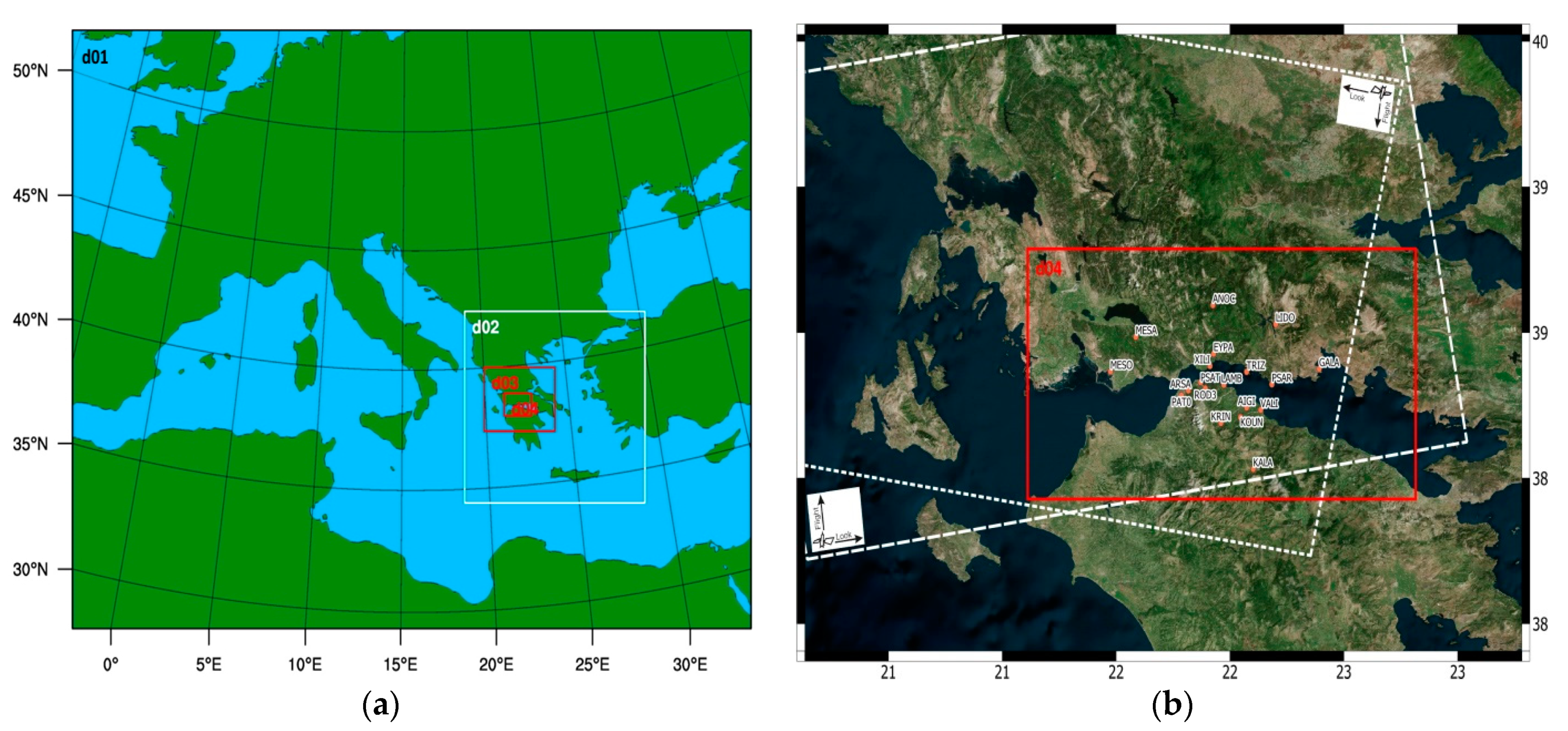
2.1. Description of the Study Area and Experimental Setup

The experiment, with the code name PaTrop (Patras–Troposphere), was implemented to provide the data needed for this study. The PaTrop test site covers an area of approximately 130 × 90 km in the region of the Western Gulf of Corinth (GoC). It is one of the most active intra-continental rifts in the world, and therefore a region with intense seismic activity. Geodetic studies conducted over the past 20 years with continuous GNSS and InSAR observations have revealed north–south extension rates up to 1.5 cm yr−1 [39,40], one of the highest worldwide. A network of GNSS stations used to monitor surface displacements in the area continuously provided the in situ zenithal tropospheric delay measurements for our study. These include nineteen permanent Topcon GB1000 and Topcon Net G3A receivers fitted with Topcon PG-A1 antennas, the locations of which are shown in Figure 1b. The stations cover a wide geographical extent while capturing a variety of different topographical and meteorological conditions (i.e., coastal, inland, or mountainous terrain) at elevations between 0 and 1020 m above sea level (ASL). This was necessary in order to account for water vapour variations resulting from orographic, coastal, and frontal gradients that could be present.
The first objective of the PaTrop experiment was to couple the zenithal tropospheric delay (ZTD) derived from GNSS data with the ZTDs derived from the output of a high-resolution meteorological model (WRF) in order to investigate the model’s capability to reproduce the tropospheric conditions that contribute to the InSAR noise signal (in particular the highly variable water vapour distribution) and provide a benchmark of real observational data for validating the model output. A series of re-analysis runs were produced to determine the best possible configuration for our study, keeping the spatial resolution of the inner domain at 1 km, which is an approach supported theoretically and practically to tackle uncertainties in high-resolution modelling [41,42]. A parametric analysis was performed for a two-week period (17–29 June 2016), during which the output of five different model configurations was tested against GNSS tropospheric measurements from the network of permanent stations in the study area [43]. The optimum model configuration which resulted from the analysis was subsequently employed to provide the data for the main part of the PaTrop experiment.

2.2. WRF Configuration and Parameterization of Physical Components

For the high-resolution dynamical downscaling simulation performed with WRF v 3.7.1 [44] over the PaTrop area of the western Gulf of Corinth, four nested domains were used (d01–d04), with a horizontal resolution of 27, 9, 3 and 1 km, respectively, as shown in Figure 1a; two-way nested, i.e., feedback from nest to its parent domain. The vertical layer distribution consisted of 45 sigma levels up to a height of about 20 km (0.1 hPa), with bottom layers being more densely populated (29 layers in the first 3 km). Boundary conditions for the model initialization were taken from the ERA-Interim global climate re-analysis database, with a 75 km horizontal resolution, 35 vertical layers and 6 h temporal resolution. The model was initiated every day from the ERA-Interim input data at 18:00 local time, producing 30 h simulations with the first 6 h being spin-up time. Model output was recorded every 30 min, from which Zenith Hydrostatic Delays (ZHD) and Zenith Wet Delays (ZWD) were calculated, which as a sum give the Zenith Total Delay according to the following equations:
ZTD (mm) = ZHD + ZWD
With:
ZHD = 2.2779 ± 0.0024   P s / f λ ,   H  
where P s is the total pressure (mbar) at the Earth’s surface, and:
f λ ,   H = 1 0.00266   c o s 2 λ 0.00028 H
accounts for the variation in gravitational acceleration with latitude λ and the height H of the surface above the ellipsoid (in km).
And:
ZWD = 0.382 ± 0.004 K 2 m b a r 1 p v T 2 d z
where p v is the water vapour pressure (mbar), and T the air temperature (K), integrated along the zenith path z. In practice, we calculated one ZWD per vertical layer, and we added the 45 values to obtain the total ZWD.
Land-use categories were taken from USGS 24-category data, which are available for different horizontal resolutions (10′, 5′, 2′, 30″). The initial land topography dataset used was the Global 30 Arc-Second Elevation Model (GTOPO30) provided by United States Geological Survey (USGS), with a 30″ resolution for the smaller domain (d04), and coarser resolutions (10′, 5′, 2′) for domains d01–d03, respectively. However, in order to test the impact of a more detailed topography on the re-analysis output, a high-resolution terrestrial dataset of d04 was later introduced (ASTER 1” global GDEM v2), with a horizontal grid of 30 m.
Five different physical parameterization schemes were tested, as listed in Table 1, in order to evaluate each scheme for its forecasting skill. The schemes were selected based on existing studies where similar high-resolution WRF simulations were used [41,45,46,47], ranging from relatively simple to more complex and computationally demanding physical parameterizations suited for high-resolution runs. There have been numerous studies validating the output of different model configurations with observations under specific conditions [41,45,46,47], showing that globally there is no optimal scheme, but rather, different schemes produce better results with respect to application, domain, season, variable, etc. Similarly, we performed a parametric analysis for a two-week period (17–29 June 2016), during which the output of the five different model configurations was validated against GNSS tropospheric measurements from 16 permanent stations in the study area (d04).

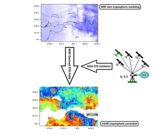
2.3. Tropospheric Correction of SAR Interferograms

Based on the results of the parametric analysis, output data from the optimal WRF high-resolution 1-km re-analysis configuration were used to calculate precise ZTD fields over the PaTrop study area, at the exact times of Sentinel-1 SAR acquisitions for the ascending track 175 and descending track 80 (i.e., 1630 and 0430 UTM, respectively). Resulting Zenith Total Delay (ZTD) values calculated from specific model output parameters (surface pressure, air temperature and water vapour profiles) were validated against a dataset of GNSS derived ZTD values, providing point measurements at the 19 points where the stations were located.
Sentinel-1 SAR data were used in this study for the generation of InSAR interferograms for 2016. The two ESA Sentinel-1 satellites (S1A and S1B) have a 6-day repeat time and carry a C-band synthetic aperture radar with a 56 mm wavelength and four operating modes. Acquisitions with a 5 × 20 m resolution in the Interferometric Wide (IW) mode were used. In total, 17 acquisitions were combined to produce 8 interferograms for the ascending (S-N) track 175 and 8 interferograms for the descending (N-S) track 80. Temporal baselines ranged from 6 days to 42 days, and perpendicular baselines were in the order of 150 m. Multilook was 6 in range and 2 in azimuth. Processing of InSAR data was done with the European Space Agency’s Sentinel Application Platform (SNAP) version 5.0 software [48], following several steps: SAR image formation, co-registration, interferogram formation, flattening (using precise orbits from ESA), and topography removing using a three arc-second (about 90 m) Shuttle Radar Topography Mission (SRTM) DEM. The final georeferenced product was resampled at 25 m using bilinear interpolation. The tropospheric correction process took place before unwrapping the interferogram. This was done in order to minimise phase ambiguities and improve the reliability of interferogram unwrapping in a region such as the western GoC, where coherence is low due to the vegetation and rough topography, which results in geometric decorrelation [49].
The InSAR observations examined are listed in Table 3. Average values of WRF vs. GNSS ZTD bias are also listed in the Table. Δbias was calculated by averaging the absolute bias (ZTDWRF–ZTDGNSS) differences between epoch 1 and epoch 2, at the 19 PaTrop stations, and is an indication of the model’s performance with respect to the observational data.
Δ b i a s = f i 1 o i 1 f i 2 o i 2 N
where fi1 and fi2 denote the model value at epochs 1 and 2, respectively, oi1 and oi2 the observational value at epochs 1 and 2, respectively, and N is the number of observations.
For the tropospheric correction, the first step was to generate differential delay maps of the total single-path tropospheric delay at the line-of-sight (LOS) at the times of the two SAR acquisitions. This was done by subtracting the 1 × 1 km single ZTD map produced by the d04 WRF output of epoch 2 from the corresponding ZTD map of epoch 1 (Figure 2). In the resulting differential delay map, LOS total delay values were calculated at each 1-km grid cell by multiplying the corresponding ZTD value with cosθ, where θ is the average incidence angle of the S1 swath in IW mode (35°). These values were then horizontally and vertically interpolated, using the weighted average inverse distance to a power gridding method, to a new 25 × 25 m grid corresponding to the pixel resolution of the interferogram. The resulting differential delay map was then wrapped (LOS total differences are converted into 2π interferometric phase fringes) and subtracted from the wrapped interferogram to produce a phase map of residuals, as illustrated in Figures 7 and 8 in the Results Section. Before the phase subtraction, the map of differential delay was “shifted” by minimizing the RMS between the two GeoTIFF maps so that their average zero phases were aligned.
All Sentinel-1 interferograms examined have temporal baselines between 6 and 42 days, ensuring the highest possible coherence and negligible amounts of crustal deformation between acquisitions. The coherence maps of both the ascending and descending tracks are shown in Figure 3. There were no major tectonic events or anthropogenic processes within the selected time series, and therefore the phase signal should mostly be attributed to tropospheric effects. Unlike historic SAR sensors, orbital errors for Sentinel-1A/B are expected to be small due to highly accurate orbit information [15].

3. Results

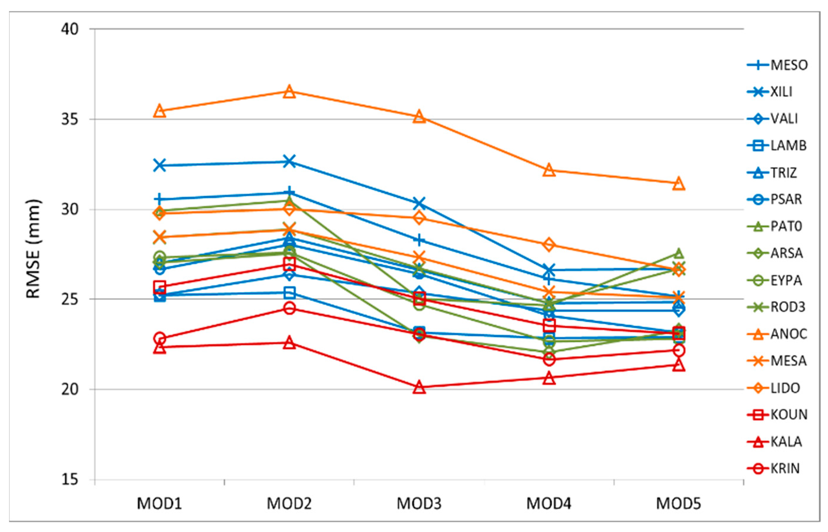
3.1. Parametric Analysis and Validation of WRF Schemes with GNSS Data

The parametric analysis was performed for a two-week period (17–29 June 2016), with the aim to test the effect of different WRF parameterization schemes on the model output. Tropospheric data (i.e., ZTD values) from the CRL GNSS network provided the benchmark for the analysis for comparison with ZTDs derived from WRF at the nearest grid point. Five different physical parameterization schemes were evaluated, as outlined in Table 2. Results were tested for their statistical significance in terms of correlation and bias with respect to the observational dataset and indicated that WRF schemes MOD4 and MOD5 exhibited a better prediction skill during the test period, with small differences between them. A summary of all validation metrics (Pearson co-efficient, mean bias, mean absolute bias and root-mean-square error) for the five parameterization schemes is presented in Table 2.
MOD5 overall exhibited the strongest correlation (Pearson correlation co-efficient R) with observations, together with a lower mean bias (MB), lower root-mean-square error (RMSE) than other parameterizations, and smaller spread of RMSE between stations than MOD4 (Figure 4). It was therefore selected as the optimum configuration for producing tropospheric delay maps for the entire PaTrop period (January–December 2016) [43].
The parametric analysis demonstrated that WRF schemes that included more complex physical parameterization (MOD4 and MOD5), although more computationally demanding, are better suited for high-resolution re-analysis simulations. The physical parameterization of MOD5 scheme included the SBU-YLin microphysics model, with a more sophisticated scheme for ice, snow, rain and graupel processes in the lower troposphere, the NOAH land surface model, the MM5 similarity scheme for surface layer physics and the YSU planetary boundary layer model. In addition, MOD4 and MOD5 used a cumulus convection scheme in both the 27-km and 9-km domains, thus simulating processes such as convective fluxes and the associated evaporation or condensation of water more coherently over a complex terrain with land-sea contrasts.

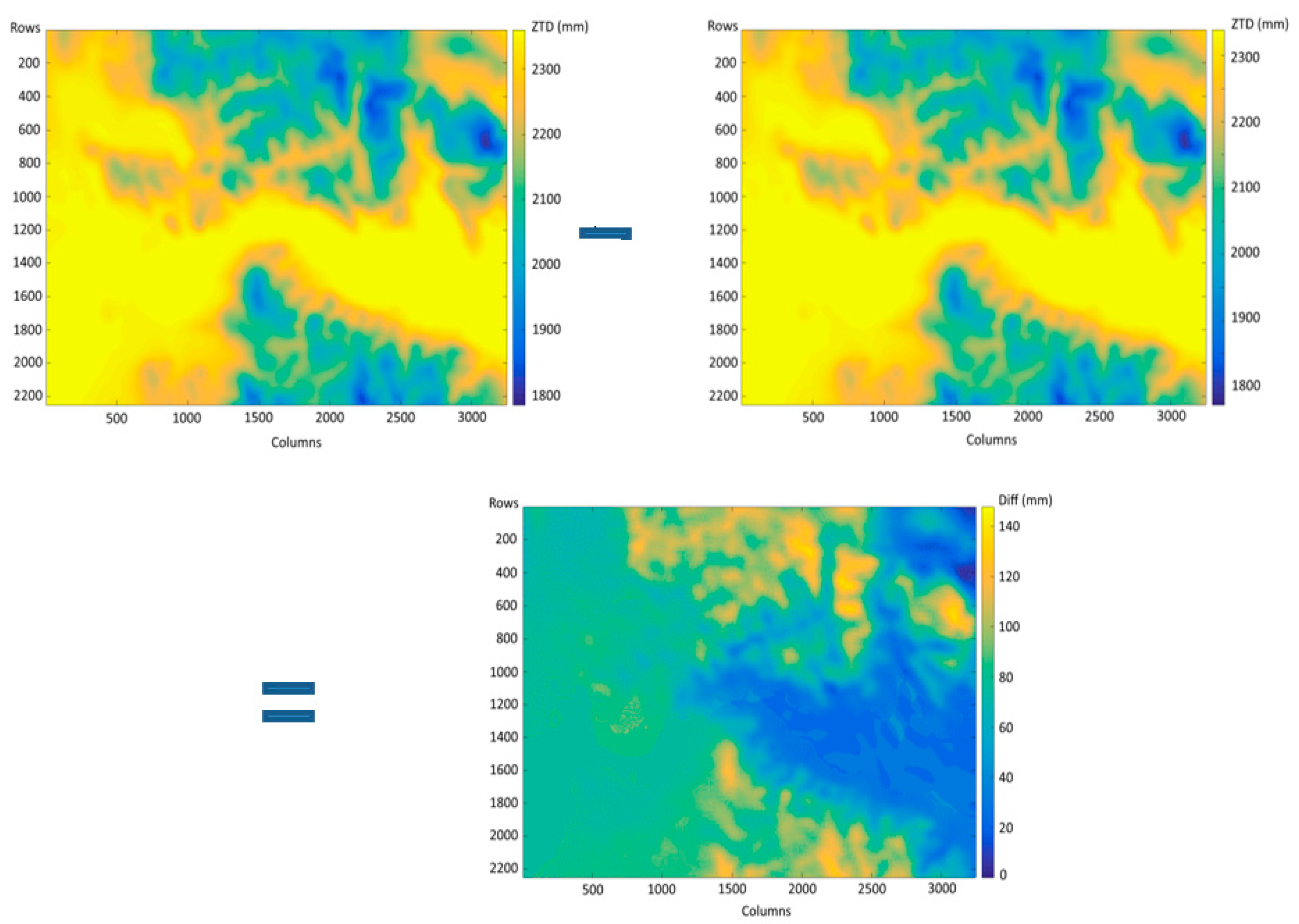
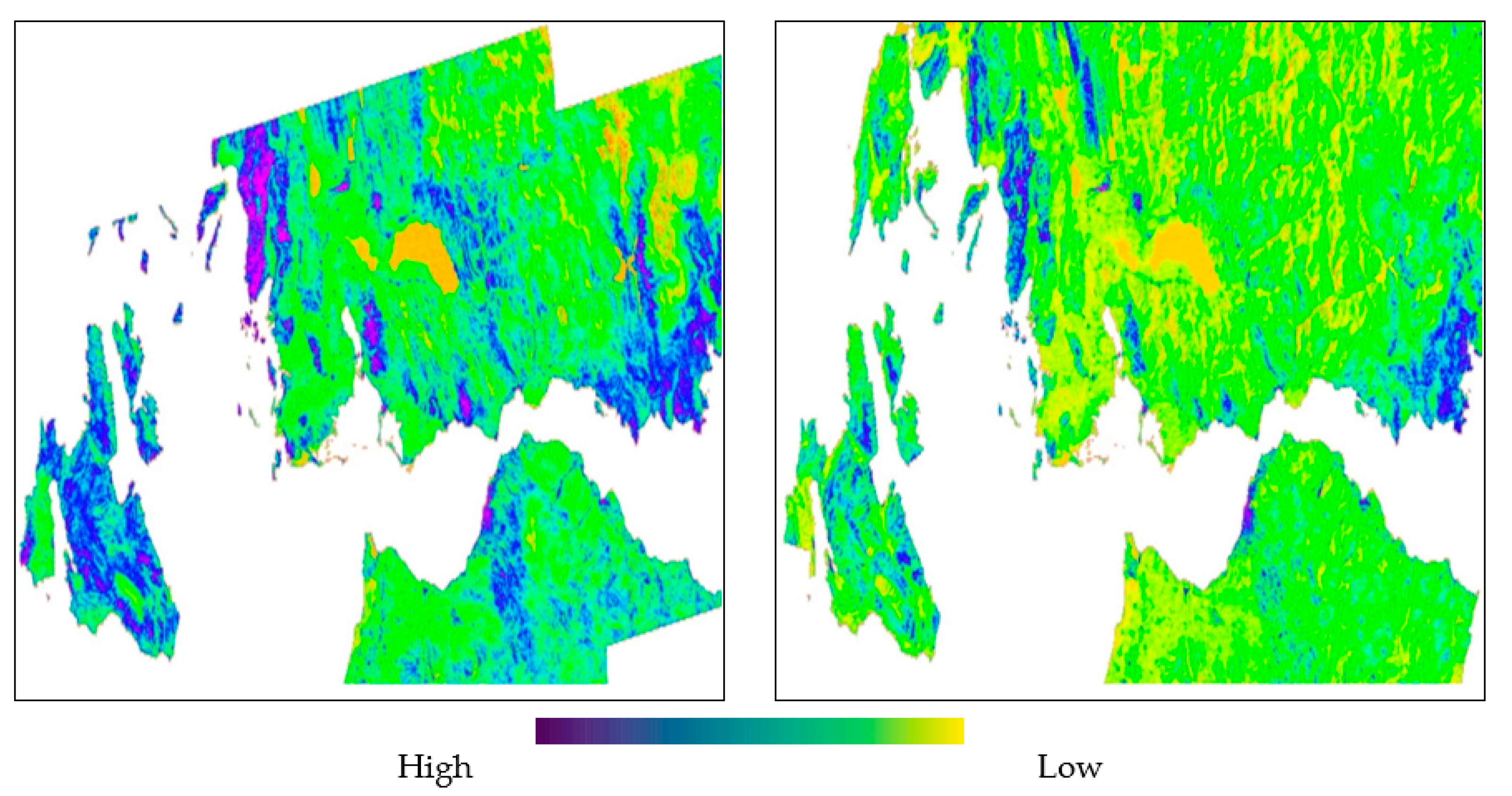
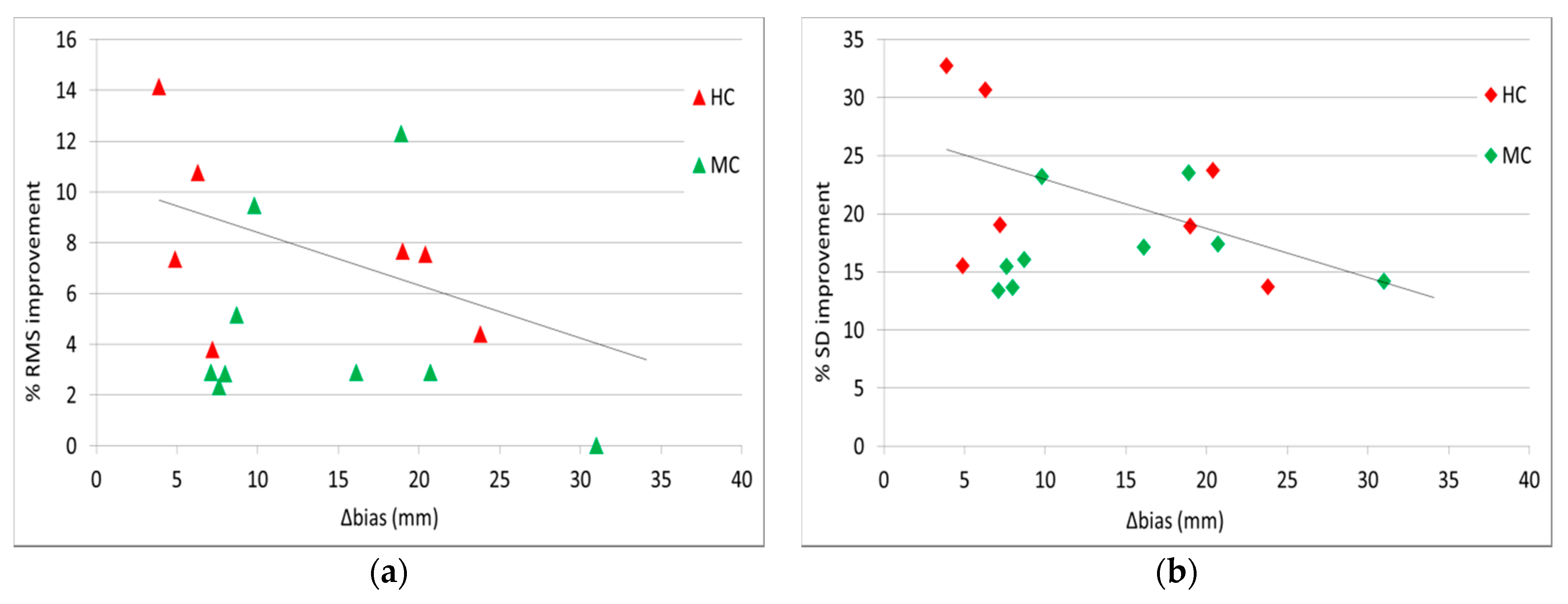
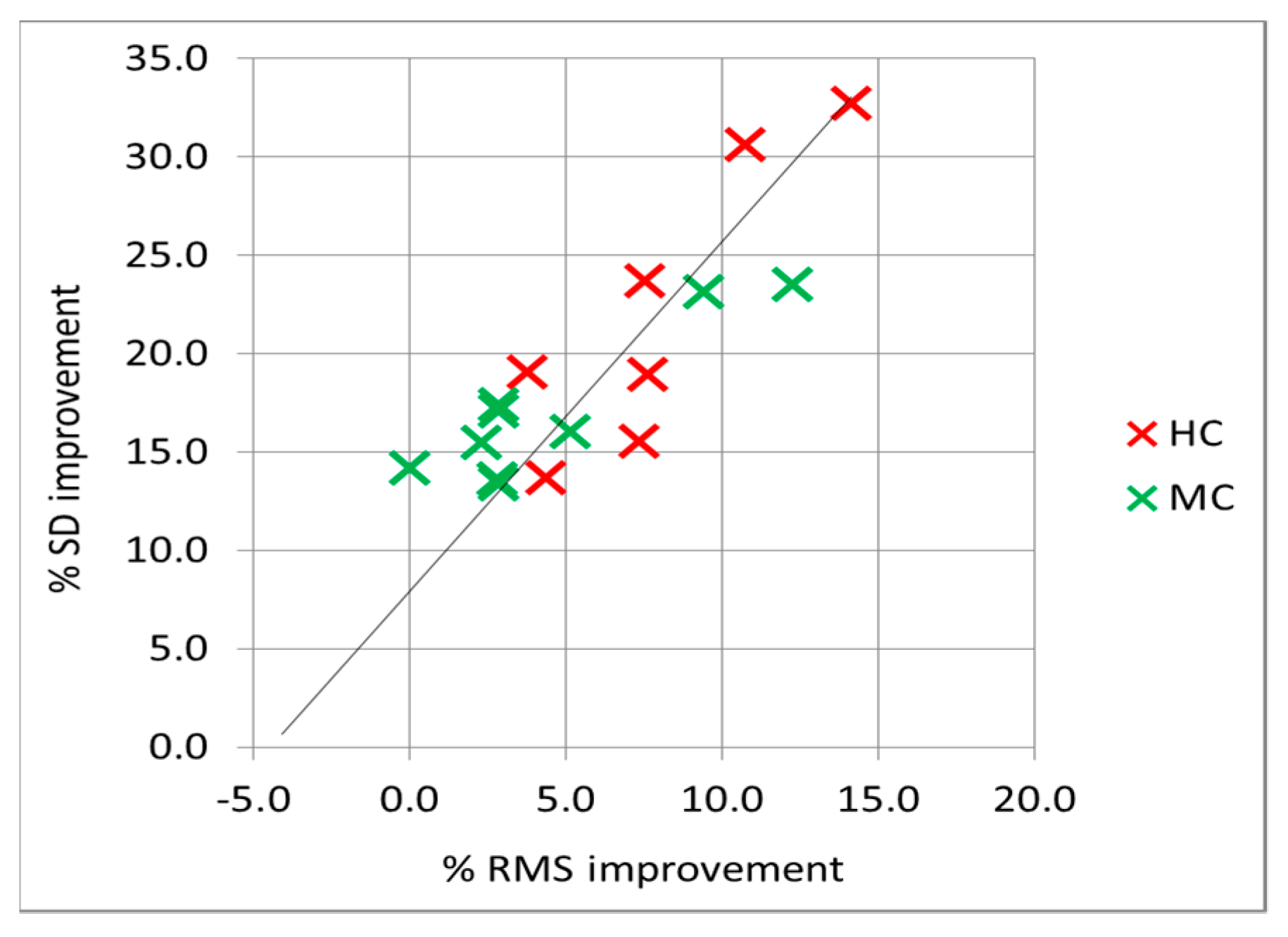
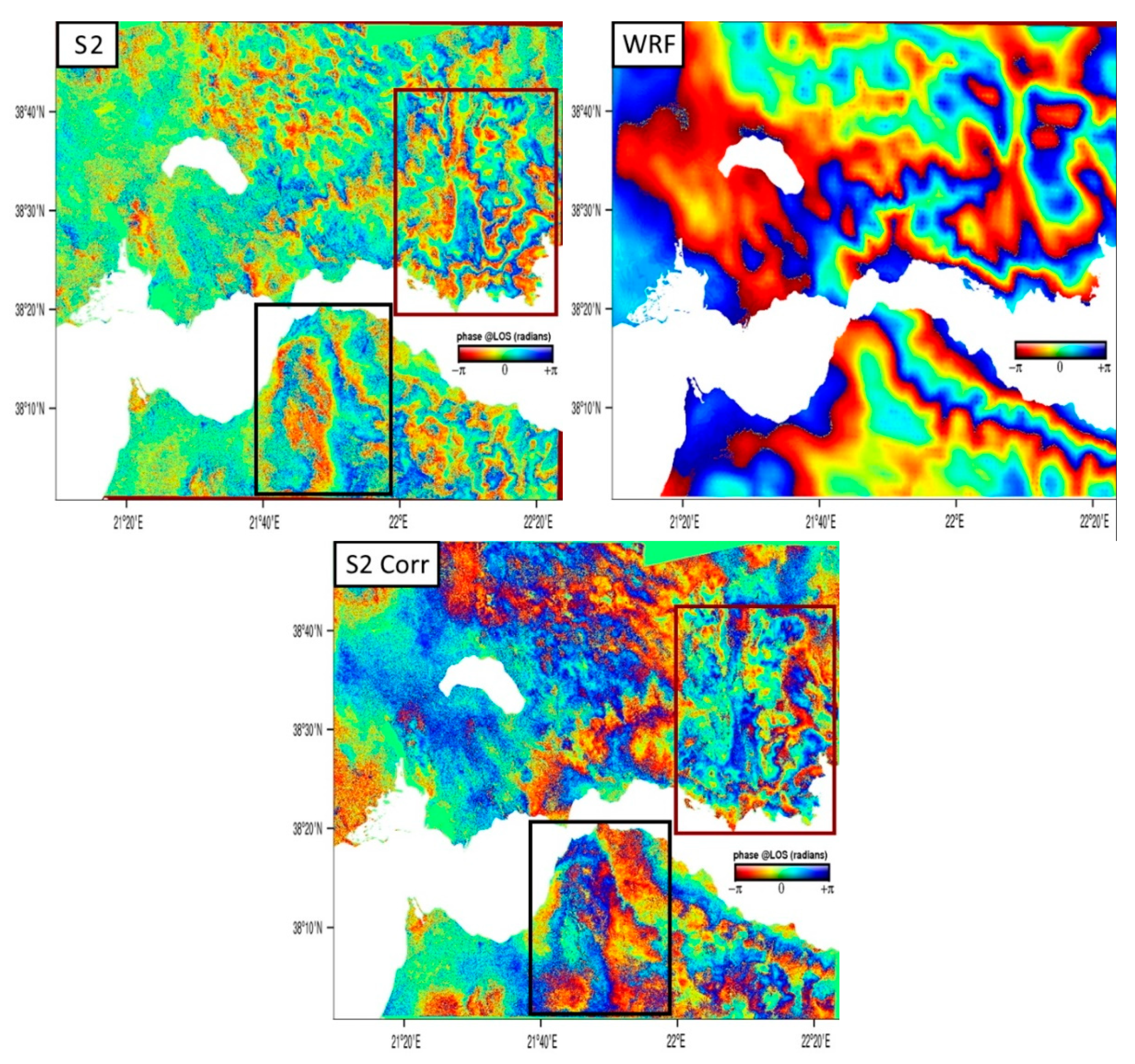
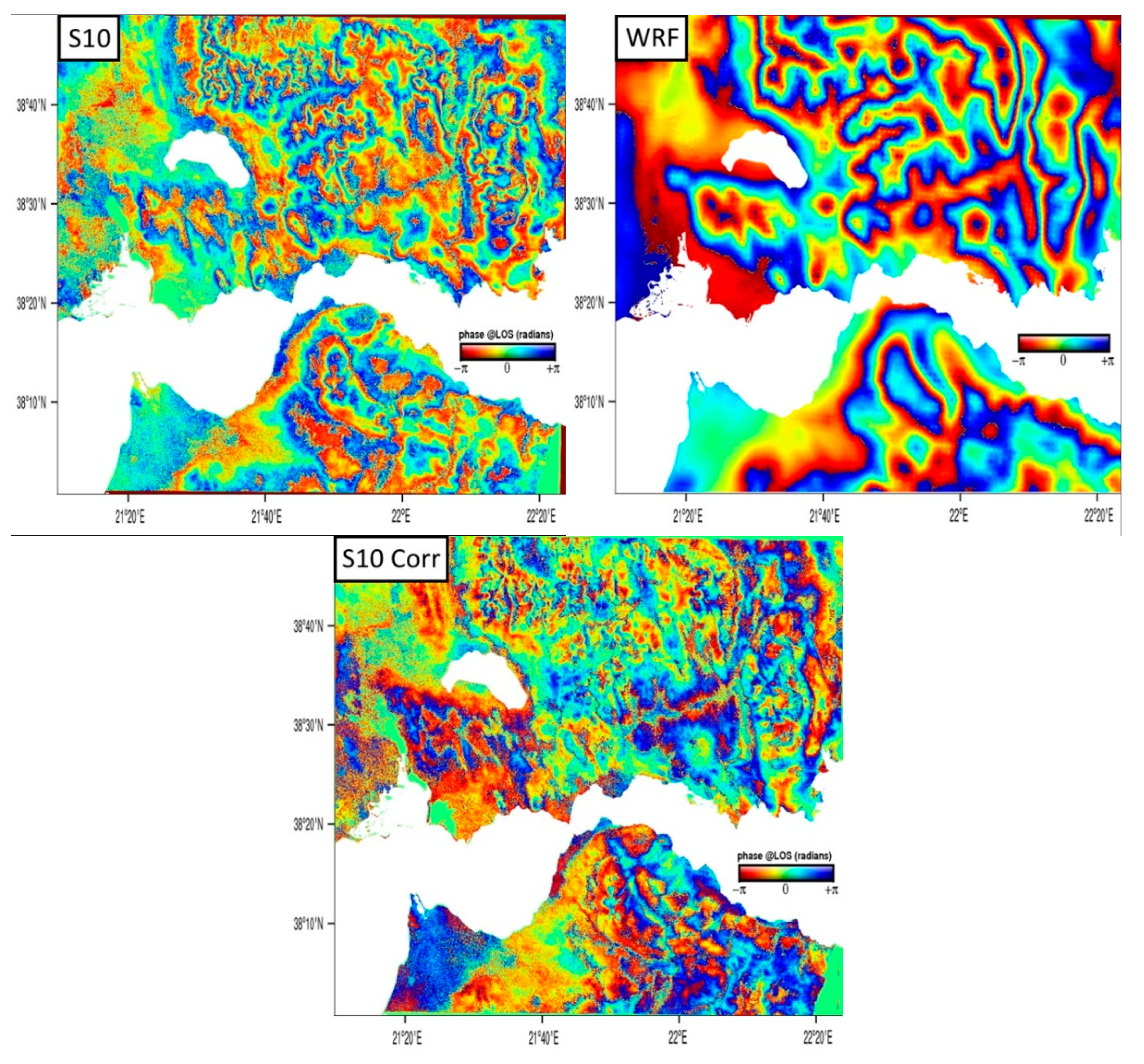
3.2. InSAR Tropospheric Correction with the Use of WRF Derived Delay Maps

In order to provide a quantitative assessment of the corrections applied in every case, the root-mean-square (RMS) and standard deviation (SD) of the phase distribution of both the original and the corrected interferograms were calculated and their differences recorded. A reduction in the RMS or SD of the wrapped interferogram after the correction was applied is a clear indication that there was a decrease in the phase gradient and fringe continuity was smoother. Table 3 lists the RMS and SD results together with the corresponding Δbias value for all 16 cases examined, while Figure 5 graphically illustrates the correlation of RMS and SD with Δbias.
In most cases, corrections applied to the wrapped interferograms with the use of high-resolution WRF-derived delay fields led to a decrease in the phase gradient, as demonstrated by the corresponding RMS and SD reductions (Table 3). The RMS of the corrected interferogram was improved in 15 out of 16 cases, with reductions ranging from 2.3% to 14.1% (6.0% on average), while SD was improved in all 16 cases, with reductions ranging from 13.4% to 32.7% (19.3% on average). Furthermore, the degree of tropospheric delay correction was correlated with WRF-GNSS average bias differences (Δbias) at the times of acquisitions. This is demonstrated in Figure 5, where the slope of the reductions in both indicators with respect to Δbias was inversely proportional. Cases with medium coherence (in green) had a slightly wider error margin than cases with high coherence (in red). When the correlation between the two indexes was plotted (Figure 6), it was confirmed that their variability was not random and that coherence was a determining factor (interferograms with high coherence are more likely to produce better tropospheric corrections).
Apart from the quantitative assessment, corrections were also assessed qualitatively, case by case, by identifying visible improvements in fringe continuity. In wrapped interferograms, the use of numerical indicators was not always adequate for assessing the degree of tropospheric phase gradient improvement due to potential problems with pixel decorrelation (low coherence) in parts of the interferogram or the existence of other components which contribute to the phase gradient. Here, two examples (out of the 16 examined) are shown, one for ascending track 175 (Figure 7) and one for descending track 80 (Figure 8). Four additional examples (Figures S1–S4) can be found in the Supplementary Materials (addendum). Case-by-case comments can be found in the legend of each figure. Summarising, we see that as a general rule, in examples where interferogram coherence is high and the forecasting skill of the WRF simulation is good, as predicted by GNSS measurements, the differential troposphere is significantly removed, and the residual phase map exhibits smoother fringe continuity. However, corrections are not always visible across the whole interferogram, first of all, because of low coherence in the western part of the image (and other parts as well), second, because of other errors (geometrical, etc.), third, because the model does not always recreate the differential atmosphere properly. More specifically, out of the sixteen interferograms that we examined: (a) in cases where coherence was good (temporal baselines usually <30 days) and Δbias was small (between 0 and 20 mm), the degree of tropospheric correction was high, resulting in a significant reduction in the density of tropospheric fringes in large sections of the interferogram, as illustrated in example S10 (Figure 8); (b) in cases where coherence was low (temporal baselines usually >30 days) and Δbias was small (between 0 and 20 mm), the degree of tropospheric correction was high only in areas with high coherence, as illustrated in example S2 (Figure 7); (c) in cases where WRF-GNSS average bias differences were high (Δbias > 20 mm), the density of tropospheric fringes was reduced at a lesser degree, and the correction was localised in smaller areas of the interferogram.

4. Discussion

High-resolution tropospheric modeling is particularly useful in the case of single interferograms, as the precise knowledge of meteorological parameters can remove the main source of error from the InSAR data, which is the delay due to the atmospheric refraction of the signal, revealing large-amplitude deformation signals (as in the case of an earthquake). In fact, it is the wet component of the delay present in the interferograms, which can be used to generate accurate maps of the atmosphere’s precipitable water vapor (PWV) over large areas [50,51], thus providing a useful tool in the domain of InSAR meteorology and vice-versa for the assimilation of interferometric SAR data into numerical weather models.
Although computationally demanding, downscaling WRF at 1 km horizontal resolution offers a detailed reconstruction of the 3-D tropospheric field over the study area, necessary for capturing small-scale atmospheric processes (such as sea breezes, orographic flows, turbulent boundary layer interactions, etc.) which cannot be captured by coarser LAMS or GAMs. Furthermore, model output was validated with the use of GNSS tropospheric data retrieved from a dense array of stations (nineteen receivers) covering the study area. Model validation with vertical column data (GNSS zenithal delays) instead of ground measurements offers the capability of evaluating the model’s forecasting skill over the entire 3-D field, thus enabling fine-tuning of its physical parameterization. It was demonstrated by the parametric analysis that schemes with a more complex physical parameterization (MOD4 and MOD5) exhibited lower bias and better correlation with respect to the GNSS observations. Additionally, turning the cumulus convection scheme on for both the 27-km and 9-km domains simulated processes, such as convective fluxes and the associated evaporation or condensation of water, more coherently over complex terrain with land-sea contrasts.
The proposed methodology was tested in a location of complex topography (western Gulf of Corinth), where the presence of highly variable water vapour signals made the removal of short-wavelength phase gradients even more challenging. Our results suggested a reduction in both long-wavelength (5–50 km) and short-wavelength (<5 km) phase delays of the wrapped phase. Residual maps exhibited a reduction in the stratified topography-correlated atmospheric signal, but most importantly, a reduction in the difficult to detect turbulent atmospheric signal (i.e., “wet” delay) in complex topographical structures of the scale of a few km, such as river incisions, valleys, etc.
Interferograms with a small temporal baseline (less than 12 days) had a higher coherence (i.e., pixel correlation between the two acquisitions) and the reduction in tropospheric “fringes” was more prominent, both visually and quantitatively. In interferograms with a larger temporal baseline, low coherence (i.e., pixel decorrelation due to system noise or terrain changes) masked many of the tropospheric artefacts. Therefore, a combination of high interferometric coherence and low Δbias (average model bias difference) between the two epochs is a good indication that the tropospheric correction will lead to a reduction in the phase gradient.

5. Conclusions

Overall, our study demonstrated the high potential and effectiveness of using high-resolution atmospheric modelling (WRF in this instance), for correcting the effects of tropospheric delay on InSAR observations and correcting atmospheric phase gradients in interferograms. The proposed methodology augments the model’s ability to predict zenithal delays in the western Gulf of Corinth, by fine-tuning its physical parameterization with the use of in situ ZTD measurements from a network of permanent GNSS stations. Furthermore, by introducing a high-resolution topography (ASTER 1s DEM), the calculation of ZTD delay fields became more accurate, and bias was minimised. The use of high-resolution Limited-Area Models (LAMs), validated by GNSS measurements, has a number of advantages over other methods which are currently used for removing the atmospheric phase screen in InSAR observations. First of all, it can be used day and night and under any weather conditions. The method can be applied in any geographical location, as long as the LAM is locally configured and parameterized. Model output data can be retrieved at the exact times of InSAR acquisitions, and the high spatial resolution (1-km) and dense vertical layering are capable of capturing near-surface atmospheric processes where complex topography is present. Finally, model validation with vertical column data (GNSS zenithal delays) instead of ground measurements offered the capability of evaluating the model’s forecasting skill over the entire 3-D field, thus enabling fine-tuning of its physical parameterization with the use of a high-accuracy representative observational dataset. This is particularly useful when it comes to estimating the highly variable water vapour signals which were exhibited in the differential atmosphere of the interferogram as densely distributed short-wavelength phase gradients.
Tropospheric corrections performed over a set of 16 wrapped Sentinel-1 interferograms with the use of high-resolution WRF-derived delay fields led to significant reductions in atmospherically-related phase gradients, with average root-mean-square and standard deviation reductions in the wrapped phase of 6.0% and 19.3%, respectively. The actual degree of correction was related to the WRF-GNSS ZTD average bias difference (Δbias) between the two acquisition epochs, and this can be a useful indicator for determining the effectiveness of the approach based on the model’s forecasting skill. Results suggest that both the stratified and the turbulent atmospheric signal can be reduced from wrapped interferograms. This is a fair improvement compared with predictive methods based on coarser GAMs, which are effective in reducing only lateral variations in stratification.
The removal of the differential tropospheric signal before the unwrapping process is beneficial for the correct estimation of the remaining noise in the interferogram. The phase ambiguity due to the aliasing of atmospheric gradients in regions of rough topography is reduced, and this minimises unwrapping errors. This will eventually lead to more reliable final products, thus enabling the detection of ground deformation signals in single interferograms (i.e., in the case of an earthquake) and improving velocity field estimates by resolving lateral variations in stratification in InSAR time series analysis.

Supplementary Materials

The following are available online at https://0-www-mdpi-com.brum.beds.ac.uk/article/10.3390/rs13122258/s1, Figure S1: and 23/11/2016, track 175 in radar geometry (top left). Corresponding WRF-derived wrapped differential LOS delay map (top right). Figure S2: 06/10/2016, track 80 in radar geometry (top left). Corresponding WRF-derived wrapped differential LOS delay map (top right). Figure S3: 18/10/2016, track 80 in radar geometry (top left). Corresponding WRF-derived wrapped differential LOS delay map (top right). Figure S4: 24/10/2016, track 80 in radar geometry (top left). Corresponding WRF-derived wrapped differential LOS delay map (top right).

Author Contributions

Conceptualization, N.R., P.E. and P.B.; Data curation, N.R., P.E., P.B. and D.K.; Formal analysis, N.R.; Funding acquisition, P.B.; Investigation, N.R. and D.K.; Methodology, N.R., P.E. and P.B.; Project administration, N.R. and P.B.; Resources, N.R. and P.B.; Software, N.R., P.E., P.B. and D.K.; Supervision, P.B., I.K., A.A.A. and A.R.; Validation, N.R., D.K. and I.K.; Visualization, N.R. and P.E.; Writing—original draft, N.R.; Writing—review & editing, N.R., P.E., P.B., D.K., I.K., A.A.A. and A.R. All authors have read and agreed to the published version of the manuscript.

Funding

This research received no external funding.

Institutional Review Board Statement

Not applicable.

Informed Consent Statement

Not applicable.

Data Availability Statement

The data presented in this study are available on request from the corresponding author. The data are not publicly available due to extensive size.

Acknowledgments

This work was supported by computational time granted from the National Infrastructures for Research and Technology S.A. (GRNET S.A.) in the National HPC facility—ARIS—under project IDs PaTrop, PaTrop2 and Atmo-InSAR-2.

Conflicts of Interest

The authors declare no conflict of interest.

References

  1. Massonnet, D.; Feigl, K.L. Radar interferometry and its application to changes in the earth’s surface. Rev. Geophys. 1998, 36, 441–500. [Google Scholar] [CrossRef] [Green Version]
  2. Hanssen, R.F. Remote Sensing and Digital Image Processing. In Radar Interferometry: Data Interpretation and Error Analysis. Earth and Environmental Science; van der Meer, F., Ed.; Kluwer Academic Publishers: Dordrecht, The Netherlands, 2001; Volume 2. [Google Scholar]
  3. Simons, M.; Fialko, Y.; Rivera, L. Coseismic deformation from the 1999 Mw 7.1 Hector Mine, California earthquake as inferred from InSAR and GPS observations. Bull. Seismol. Soc. Am. 2002, 92, 1390–1402. [Google Scholar] [CrossRef]
  4. Lasserre, C.; Peltzer, G.; Crampe, F.; Klinger, Y.; Van der Woerd, J.; Tapponnier, P. Coseismic deformation of the 2001 Mw = 7.8 Kokoxili earthquake in Tibet, measured by synthetic aperture radar interferometry. J. Geophys. Res. 2005, 110, B12408. [Google Scholar] [CrossRef] [Green Version]
  5. Briole, P.; Elias, P.; Parcharidis, I.; Bignami, C.; Benekos, G.; Samsonov, S.; Kyriakopoulos, C.; Stramondo, S.; Chamot-Rooke, N.; Drakatou, M.L.; et al. The seismic sequence of January–February 2014 at Cephalonia Island (Greece): Constraints from SAR interferometry and GPS. Geophys. J. Int. 2015, 203, 1528–1540. [Google Scholar] [CrossRef] [Green Version]
  6. Lundgren, P.; Casu, F.; Manzo, M.; Pepe, A.; Berardino, P.; Sansosti, E.; Lanari, R. Gravity and magma induced spreading of Mount Etna volcano revealed by satellite radar interferometry. Geophys. Res. Lett. 2004, 31, L04602. [Google Scholar] [CrossRef] [Green Version]
  7. Doubre, C.; Peltzer, G. Fluid-controlled faulting process in the Asal Rift, Djibouti, from 8 yr of radar interferometry observations. Geology 2007, 35, 69–72. [Google Scholar] [CrossRef]
  8. Grandin, R.; Socquet, A.; Doin, M.P.; Jacques, E.; De Chabalier, B.; King, G.C.P. Transient rift opening in response to multiple dike injections in the Manda Hararo rift (Afar, Ethiopia) imaged by time-dependent elastic inversion of interferometric synthetic aperture radar data. J. Geophys. Res. 2010, 115, B09403. [Google Scholar] [CrossRef] [Green Version]
  9. Elliott, J.R.; Biggs, J.; Parsons, B.; Wright, T.J. InSAR slip rate determination on the Altyn Tagh Fault, northern Tibet, in the presence of topographically correlated atmospheric delays. Geophys. Res. Lett. 2008, 35, L12309. [Google Scholar] [CrossRef] [Green Version]
  10. Walters, R.J.; Elliott, J.R.; Parsons, B.; Li, Z. Rapid strain accumulation on the Ashkabad fault (Turkmenistan) from atmosphere-corrected InSAR. J. Geophys. Res. Solid Earth 2013, 118, 3674–3690. [Google Scholar] [CrossRef] [Green Version]
  11. Chen, M.; Tomás, R.; Li, Z.; Motagh, M.; Li, T.; Hu, L.; Gong, H.; Li, X.; Yu, J.; Gong, X. Imaging land subsidence induced by groundwater extraction in Beijing (China) using satellite radar interferometry. Remote Sens. 2016, 8, 468. [Google Scholar] [CrossRef] [Green Version]
  12. Short, N.; LeBlanc, A.M.; Sladen, W.; Oldenborger, G.; Mathon-Dufour, V.; Brisco, B. RADARSAT-2 D-InSAR for ground displacement in permafrost terrain, validation from Iqaluit Airport, Baffin Island, Canada. Remote Sens. Environ. 2014, 141, 40–51. [Google Scholar] [CrossRef]
  13. Zebker, H.; Villasenor, J. Decorrelation in interferometric radar echoes. IEEE Trans. Geosci. Remote Sens. 1992, 30, 950–959. [Google Scholar] [CrossRef] [Green Version]
  14. Tarayre, H.; Massonnet, D. Atmospheric propagation heterogeneities revealed by ERS-1 interferometry. Geophys. Res. Lett. 1996, 23, 989–992. [Google Scholar] [CrossRef]
  15. Fattahi, H.; Amelung, F. InSAR bias and uncertainty due to the systematic and stochastic tropospheric delay. J. Geophys. Res. Solid Earth 2015, 120, 8758–8773. [Google Scholar] [CrossRef] [Green Version]
  16. Fattahi, H.; Amelung, F. DEM error correction in InSAR time series. IEEE Trans. Geosci. Remote Sens. 2013, 51, 4249–4259. [Google Scholar] [CrossRef]
  17. Wright, T.; Parsons, B.; Fielding, E. Measurement of interseismic strain accumulation across the North Anatolian Fault by satellite radar interferometry. Geophys. Res. Lett. 2001, 28, 2117–2120. [Google Scholar] [CrossRef]
  18. Béjar-Pizarro, M.; Socquet, A.; Armijo, R.; Carrizo, D.; Genrich, J.; Simons, M. Interseismic coupling and Andean structure in the north Chile subduction zone. Nat. Geosci. 2013, 6, 462–467. [Google Scholar] [CrossRef] [Green Version]
  19. Jolivet, R.; Agram, P.S.; Lin, N.Y.; Simons, M.; Doin, M.P.; Peltzer, G.; Li, Z. Improving InSAR geodesy using Global Atmospheric Models. J. Geophys. Res. Solid Earth 2014, 119, 2324–2341. [Google Scholar] [CrossRef]
  20. Wicks, C.; Dzurisin, D.; Ingebritsen, S.; Thatcher, W.; Lu, Z.; Iverson, J. Magmatic activity beneath the quiescent Three Sisters volcanic center, central Oregon Cascade Range, USA. Geophys. Res. Lett. 2002, 29, 26-1–26-4. [Google Scholar] [CrossRef] [Green Version]
  21. Lin, Y.N.; Simons, M.; Hetland, E.A.; Muse, P.; DiCaprio, C.A. Multiscale approach to estimating topographically correlated propagation delays in radar interferograms. Geochem. Geophys. Geosyst. 2010, 11, Q09002. [Google Scholar] [CrossRef]
  22. Bekaert, D.P.S.; Walters, R.J.; Wright, T.J.; Hooper, A.; Parker, D.J. Statistical comparison of InSAR tropospheric correction techniques. Remote Sens. Environ. 2015, 170, 40–47. [Google Scholar] [CrossRef] [Green Version]
  23. Delacourt, C.; Briole, P.; Achache, J.A. Tropospheric corrections of SAR interferograms with strong topography. Application to Etna. Geophys. Res. Lett. 1998, 25, 2849–2852. [Google Scholar] [CrossRef]
  24. Webley, P.W.; Bingley, R.M.; Dodson, A.H.; Wadge, G.; Waugh, S.J.; James, I.N. Atmospheric water vapour correction to InSAR surface motion measurements on mountains: Results from a dense GPS network on Mount Etna. Phys. Chem. Earth 2002, 27, 363–370. [Google Scholar] [CrossRef]
  25. Li, Z.; Muller, J.; Cross, P.; Fielding, E. Interferometric synthetic aperture radar (InSAR) atmospheric correction: GPS, Moderate Resolution Imaging Spectroradiometer (MODIS), and InSAR integration. J. Geophys. Res. 2005, 110. [Google Scholar] [CrossRef]
  26. Löfgren, J.; Björndahl, F.; Moore, A.; Webb, F.; Fielding, E.; Fishbein, E. Tropospheric correction for InSAR using interpolated ECMWF data and GPS Zenith Total Delay from the Southern California Integrated GPS Network. In Proceedings of the Geoscience and Remote Sensing Symposium (IGARSS) 2010 IEEE International, Honolulu, HI, USA, 25–30 July 2010; pp. 4503–4506. [Google Scholar] [CrossRef] [Green Version]
  27. Li, Z.; Fielding, E.; Cross, P.; Preusker, R. Advanced InSAR atmospheric correction: MERIS/MODIS combination and stacked water vapour models. Int. J. Remote Sens. 2009, 30, 3343–3363. [Google Scholar] [CrossRef]
  28. Xu, W.; Li, Z.; Ding, X.; Feng, G.; Hu, D.; Long, J.; Yin, H.; Yang, E. Correcting atmospheric effects in ASAR interferogram with MERIS integrated water vapor data. Chin. J. Geophys. 2010, 53, 1073–1084. [Google Scholar]
  29. Doin, M.P.; Lasserre, C.; Peltzer, G.; Cavali, O.; Doubre, C. Corrections of stratified tropospheric delays in SAR interferometry: Validation with global atmospheric models. J. Appl. Geophys. 2009, 69, 35–50. [Google Scholar] [CrossRef]
  30. Wadge, G.; Zhu, M.; Holley, R.; James, I.; Clark, P.; Wang, C.; Woodage, M. Correction of Atmospheric Delay Effects in Radar Interferometry Using a Nested Mesoscale Atmospheric Model. J. Appl. Geophys. 2010, 72, 141–149. [Google Scholar] [CrossRef]
  31. Foster, J.; Kealy, J.; Cherubini, T.; Businger, S.; Lu, Z.; Murphy, M. The utility of atmospheric analyses for the mitigation of artifacts in InSAR. J. Geophys. Res. Solid Earth 2013, 118, 748–758. [Google Scholar] [CrossRef] [Green Version]
  32. Kinoshita, Y.; Furuya, M.; Hobiger, T.; Ichikawa, R. Are numerical weather model outputs helpful to reduce tropospheric delay signals in InSAR data? J. Geod. 2013, 87, 267–277. [Google Scholar] [CrossRef] [Green Version]
  33. Puysségur, B.; Michel, R.; Avouac, J.P. Tropospheric phase delay in interferometric synthetic aperture radar estimated from meteorological model and multispectral imagery. J. Geophys. Res. 2007, 112, B05419. [Google Scholar] [CrossRef] [Green Version]
  34. Yu, C.; Li, Z.; Penna, N.T. Interferometric synthetic aperture radar atmospheric correction using a GPS-based iterative tropospheric decomposition model. Remote Sens. Environ. 2018, 204, 109–121. [Google Scholar] [CrossRef]
  35. Li, Z.; Muller, J.; Cross, P.; Albert, P.; Fischer, J.; Bennartz, R. Assessment of the potential of MERIS near—infrared water vapour products to correct ASAR interferometric measurements. Int. J. Remote Sens. 2006, 27, 349–365. [Google Scholar] [CrossRef] [Green Version]
  36. Eff-Darwich, A.; Perez, J.; Fernandez, J.; Garcia-Lorenzo, B. Using a mesoscale meteorological model to reduce the effect of tropospheric water vapour from DInSAR data: A case study for the island of Tenerife. Pure Appl. Geophys. 2012, 169, 1425–1441. [Google Scholar] [CrossRef]
  37. Yun, Y.; Zeng, Q.; Green, B.W.; Zhang, F. Mitigating atmospheric effects in InSAR measurements through high-resolution data assimilation and numerical simulations with a weather prediction model. Int. J. Remote Sens. 2015, 36, 2129–2147. [Google Scholar] [CrossRef]
  38. Nico, G.; Tomé, R.; Catalão, J.; Miranda, P.M.A. On the use of the WRF model to mitigate tropospheric phase delay effects in SAR Interferograms. IEEE Trans. Geosci. Remote Sens. 2011, 49, 4970–4976. [Google Scholar] [CrossRef]
  39. Briole, P.; Rigo, A.; Lyon-Caen, H.; Ruegg, J.C.; Papazissi, K.; Mitsakaki, C.; Balodimou, A.; Veis, G.; Hatzfeld, D.; Deschamps, A. Results from repeated Global Positioning System surveys between 1990 and 1995. J. Geophys. Res. 2000, 105, 25605–25625. [Google Scholar] [CrossRef] [Green Version]
  40. Avallone, A.; Briole, P.; Agatza-Balodimou, A.M.; Billiris, H.; Charade, O.; Mitsakaki, C.; Nercessian, A.; Papazissi, K.; Paradissis, D.; Veis, G. Analysis of eleven years of deformation measured by GPS in the Corinth Rift Laboratory area. Comptes Rendus Geosci. 2004, 336, 301–312. [Google Scholar] [CrossRef] [Green Version]
  41. Kioutsioukis, I.; De Meij, A.; Jakobs, H.; Katragkou, E.; Vinuesa, J.F.; Kazantzidis, A. High resolution WRF ensemble forecasting for irrigation: Multi-variable evaluation. Atmos. Res. 2015, 167, 156–174. [Google Scholar] [CrossRef]
  42. Garcia-Diez, M.; Fernandez, J.; Vautard, R. An RCM multi-physics ensemble over Europe: Multi-variable evaluation to avoid error compensation. Clim. Dyn. 2015, 45, 3141–3156. [Google Scholar] [CrossRef] [Green Version]
  43. Roukounakis, N.; Katsanos, D.; Briole, P.; Elias, P.; Kioutsioukis, I.; Argiriou, A.A.; Retalis, A. Use of GNSS Tropospheric Delay Measurements for the Parameterization and Validation of WRF High-Resolution Re-Analysis over the Western Gulf of Corinth, Greece: The PaTrop Experiment. Remote Sens. 2021, 13, 1898. [Google Scholar] [CrossRef]
  44. Skamarock, W.; Klemp, J.B.; Dudhia, J.; Gill, D.O.; Barker, D.; Duda, M.G.; Huang, X.-Y.; Wang, W. A Description of the Advanced Research WRF Version 3. NCAR Technical Note NCAR/TN-475 + STR.; University Corporation for Atmospheric Research: Boulder, CO, USA, 2008. [Google Scholar] [CrossRef]
  45. Mooney, P.A.; Mulligan, F.J.; Fealy, R. Evaluation of the sensitivity of the weather research and forecasting model to parameterization schemes for regional climates of Europe over the period 1990–1995. J. Clim. 2013, 26, 1002–1017. [Google Scholar] [CrossRef] [Green Version]
  46. Kotlarski, S.; Keuler, K.; Christensen, O.B.; Colette, A.; Déqué, M.; Gobiet, A.; Goergen, K.; Jacob, D.; Lüthi, D.; van Meijgaard, E.; et al. Regional climate modeling on European scales: A joint standard evaluation of the EURO-CORDEX RCM ensemble. Geosci. Model Dev. 2014, 7, 1297–1333. [Google Scholar] [CrossRef] [Green Version]
  47. Garcia-Diez, M.; Fernandez, J.; Fita, L.; Yague, C. Seasonal dependence of WRF model biases and sensitivity to PBL schemes over Europe, Q.J.R. Meteorol. Soc. 2013, 139, 501–514. [Google Scholar] [CrossRef] [Green Version]
  48. Yague-Martinez, N.; Prats-Iraola, P.; Rodríguez González, F.; Brcic, R.; Shau, R.; Geudtner, D.; Eineder, M.; Bamler, R. Interferometric Processing of Sentinel-1 TOPS Data. IEEE Trans. Geosci. Remote Sens. 2016, 54, 2220–2234. [Google Scholar] [CrossRef] [Green Version]
  49. Pinel, V.; Hooper, A.; De la Cruz-Reyna, S.; Reyes-Davila, G.; Doin, M.; Bascou, P. The challenging retrieval of the displacement field from InSAR data for andesitic stratovolcanoes: Case study of Popocatepetl and Colima volcano, Mexico. J. Volcanol. Geotherm. Res. 2011, 200, 49–61. [Google Scholar] [CrossRef]
  50. Alshawaf, F.; Hinz, S.; Mayer, M.; Meyer, F.J. Constructing accurate maps of atmospheric water vapor by combining interferometric synthetic aperture radar and GNSS observations. J. Geophys. Res. Atmos. 2015, 120, 1391–1403. [Google Scholar] [CrossRef]
  51. Mateus, P.; Catalão, J.; Nico, G. Sentinel-1 interferometric SAR mapping of precipitable water vapor over a country-spanning area. IEEE Trans. Geosci. Remote Sens. 2017, 55, 2993–2999. [Google Scholar] [CrossRef]
Figure 1. (a) Map showing the four nested domains (d01-d04) used for WRF weather re-analysis over the Western GoC (left). (b) Map of the PaTrop study area, Western GoC (right). The CRL network of permanent GNSS stations is shown, along with the SAR swaths of the two Sentinel-1 satellites on ascending track 175 and descending track 80. The red box indicates the location of the 1 × 1 km inner domain of the WRF re-analysis run (Domain d04).
Remotesensing 13 02258 g001
Figure 2. Example of producing a differential ZTD map from the subtraction of two single ZTD maps (epoch 1–epoch 2), produced with WRF at the times of InSAR acquisitions. Pair corresponds to dates 18–30 September 2016. The size of the area is 130 × 90 km, corresponding to the inner WRF domain d04. The resulting differential ZTD map is then converted to LOS total delay map and wrapped (arithmetic values were transformed into 2π phase values) to correct the corresponding interferogram.
Remotesensing 13 02258 g002
Figure 3. Coherence maps for Sentinel-1 ascending track 175 (left) and descending track 80 (right) over the extended western GoC area. Purple colour indicates highest, and yellow indicates lowest coherence.
Remotesensing 13 02258 g003
Figure 4. RMSE distribution at the 16 stations, for each model configuration. Stations are colour-coded, according to their location: blue—coastal; green—inland; orange—upland north; red—upland south.
Remotesensing 13 02258 g004
Figure 5. (a) Correlation of RMS reduction between original and corrected interferograms and Δbias. (b) Correlation of SD reduction between original and corrected interferograms and Δbias. Colours correspond to coherence (red = high, green = medium).
Remotesensing 13 02258 g005
Figure 6. Correlation of % SD reduction vs. % RMS reduction for the 16 cases studied. Colours correspond to coherence (red = high, green = medium).
Remotesensing 13 02258 g006
Figure 7. Wrapped interferogram from SAR acquisitions on 30 September 2016 and 24 October 2016, track 175 in radar geometry (top left). Corresponding WRF-derived wrapped differential LOS delay map (top right). The correlation between interferogram and meteogram is directly visible, for example, in the Mornos valley (red box) or around the Panachaikon mountain (black box) as the model’s forecasting skill was high in both acquisition epochs (Δbias low). The wrapped differential LOS delay map generated from WRF output data was subtracted from the corresponding wrapped interferogram to produce a map of residual 2π phase cycles (bottom). The resulting residual map, in this case, demonstrates tropospheric corrections in several areas of the interferogram where coherence was high, leading to a decrease in the phase gradient.
Remotesensing 13 02258 g007
Figure 8. Wrapped interferogram from SAR acquisitions on 18 September 2016 and 30 September 2016, track 80 in radar geometry (top left). Corresponding WRF-derived wrapped differential LOS delay map (top right). An example of good consistency between WRF and GNSS is also reflected in the good correlation between the interferogram and the delay map, with short and long wavelengths being observed. In the corresponding residual map after subtraction of WRF-derived wrapped differential LOS delay map from the interferogram (bottom), good tropospheric corrections and an overall reduction in the phase gradient were observed across the whole extent of the interferogram.
Remotesensing 13 02258 g008
Table 1. WRF parameterization options used for the PaTrop sensitivity analysis.
MOD1MOD2MOD3MOD4MOD5
Microphysics (mp)WSM3 Morrison MorrisonMorrisonSBU-YLin
Land surface (sf)NOAH NOAH Pleim–Xiu Pleim–Xiu NOAH
Surface layer physics (sfclay)Monin–ObukhovMonin–ObukhovPleim–Xiu Pleim–Xiu MM5 similarity
Radiation physics (sw)Dudhia Dudhia DudhiaDudhiaDudhia
Radiation physics (lw)RRTM RRTM RRTMRRTMRRTM
Planetary boundary layer physics (pbl)MYJ MYJ ACM2ACM2YSU
Cloud physics (cu)Kain–Fritsch at 27 kmKain–Fritsch at 27 kmKain–Fritsch at 27 kmKain–Fritsch at 27 and 9 kmKain–Fritsch at 27 and 9 km
Table 2. Statistical indexes of WRF ZTD vs. GNSS ZTD time series—17–29 June 2016.
WRF SchemeRMB (mm)MAB (mm)RMSE (mm)
MOD10.69−14.921.427.8
MOD20.69−15.921.928.5
MOD30.73−14.920.726.2
MOD40.73−11.819.424.6
MOD50.74−11.619.524.4
Table 3. Dates of Sentinel-1 interferograms examined, corresponding WRF vs. GNSS ZTD average bias differences (Δbias), and RMS and SD differences between original and corrected interferograms.
IfgTrackDatesΔbias (mm)RMS % ReductionSD % Reduction
117530/09–06/1020.47.523.7
217530/09–24/107.12.913.4
317530/09–05/1120.72.917.4
417506/10–24/1016.12.917.1
517524/10–05/11197.718.9
617524/10–17/119.89.423.2
717524/10–23/118.02.813.7
817524/10–05/128.75.116.0
98025/08–18/0931.00.014.2
108018/09–30/097.23.819.0
118018/09–06/1023.84.413.7
128018/09–18/1018.912.323.5
138006/10–24/107.62.315.5
148018/10–24/104.97.315.5
158017/11–23/116.310.830.6
168005/12–11/123.914.132.7
Publisher’s Note: MDPI stays neutral with regard to jurisdictional claims in published maps and institutional affiliations.

