Article

Space-Time Evolutions of Land Subsidence in the Choushui River Alluvial Fan (Taiwan) from Multiple-Sensor Observations

1
Department of Earth Sciences, National Central University, Taoyuan 32001, Taiwan
2
Green Environmental Engineering Consultant Co. LTD, Hsinchu 31057, Taiwan
3
Center for Space and Remote Sensing Research, National Central University, Taoyuan 32001, Taiwan
4
Department of Civil Engineering, National Yang Ming Chiao Tung University, Hsinchu 30010, Taiwan
5
Department of Natural Resource and Environmental Studies, National Dong Hwa University, Hualien 97401, Taiwan
6
Research Center for Environmental Changes, Academia Sinica, Taipei 11529, Taiwan
*
Author to whom correspondence should be addressed.
Remote Sens. 2021, 13(12), 2281; https://0-doi-org.brum.beds.ac.uk/10.3390/rs13122281
Submission received: 4 May 2021 / Revised: 31 May 2021 / Accepted: 7 June 2021 / Published: 10 June 2021
(This article belongs to the Special Issue Remote Sensing Approaches to Groundwater Management and Mapping)

Abstract

:
Land subsidence is a significant problem around the world that can increase the risk of flooding, damage to infrastructure, and economic loss. Hence, the continual monitoring of subsidence is important for early detection, mechanism understanding, countermeasure implementation, and deformation prediction. In this study, we used multiple-sensor observations from the Continuous Global Positioning System (CGPS), the small baseline subset (SBAS) algorithm, interferometric synthetic-aperture radar (InSAR), precise leveling, multi-layer compaction monitoring wells (MLCWs), and groundwater observation wells (GWs) to show the spatial and temporal details of land subsidence in the Choushui River alluvial fan (CRAF), Taiwan, from 1993 to 2019. The results showed that significant land subsidence has occurred along the coastal areas in the CRAF, and most of the inland subsidence areas have also experienced higher subsidence rates (>30 mm/yr). The analysis of subsidence along the Taiwan High Speed Rail (THSR) revealed a newly formed subsidence center between Tuku and Yuanchang Townships in Yunlin, with high subsidence rates ranging from 30 to 70 mm/yr. We propose a map showing, for the first time, the distribution of deep compactions occurring below 300 m depth in the CRAF.

Graphical Abstract

1. Introduction

Land subsidence caused primarily by anthropogenic developments is becoming a severe problem around the world [1,2,3,4,5,6,7]. Manmade land subsidence mainly results from groundwater depletion. When groundwater extraction persistently exceeds the natural recharge limit, the extraction leads to groundwater level decline, sea-water intrusion, groundwater quality deterioration, land subsidence, poor drainage, and flooding. There are 200 locations in 34 countries that suffer land subsidence because of groundwater depletion during the past century. Nineteen percent of the global population may face a high risk of subsidence in the following decades [3].
In Taiwan, the rapid growth of the population and economy increased groundwater demand and motivated groundwater overextraction. Currently, the region of the Choushui River alluvial fan (CRAF) in central Taiwan has extensive and severe land subsidence due to unregulated groundwater pumping and slow natural groundwater recharge [8,9,10,11,12,13]. Since 1995, a long-term and systematic project funded by the Water Resources Agency (WRA), Taiwan, has been underway to monitor land subsidence in the CRAF using precise leveling, the Continuous Global Positioning System (CGPS), multi-layer compaction monitoring wells (MLCWs), and groundwater observation wells (GWs). The outcome of the project provides the needed information for the WRA to take measures to mitigate land subsidence, such as restricting groundwater pumping, increasing forests, and constructing dams.
Previous geodetic sensors, such as GPS and leveling, provide accurate but only sparse point-wise measurements. Hence, the spatiotemporal distribution pattern of land subsidence cannot be identified comprehensively, especially in areas where no monitoring sensors have been established. In order to rapidly and efficiently obtain the information on wide-range subsidence with high spatial and temporal resolution, interferometric synthetic-aperture radar (InSAR) has been applied to detect ground deformations at sub-centimeter accuracy levels [1,2,4,6,14,15,16,17,18,19]. However, InSAR-derived deformations are often contaminated by atmospheric disturbance and spatial and temporal decorrelation of surface properties in SAR images. To reduce these contaminations, methods for extracting deformations at multiple epochs have been proposed, such as persistent scatterer interferometry (PSI) [20,21,22] and the small baseline subset (SBAS) algorithm [6,23,24], which function based on temporal, spatial, and statistical analyses of SAR images.
Numerous SAR-based studies on land subsidence monitoring in the CRAF have been recently published. For example, Hung et al. [4] used multiple sensors to monitor land subsidence from 2006 to 2007, including precise leveling, GPS, MLCWs, and DInSAR. The land subsidence results from leveling, GPS, and DInSAR were consistent. The difference in vertical displacement between the leveling and GPS results was within 1 cm and between the leveling and DInSAR results it was within 1–2 cm, respectively. Furthermore, many minor and locally distributed displacements in Yunlin not detected by leveling appeared in the PSI and Envisat results. The maximum annual displacement rates of up to 7–8 cm/yr occurred over the period 2006–2008 [5]. Tung and Hu [25] applied PSInSAR to estimate the land subsidence in the CRAF from 1996 to 1999. Their results revealed several subsidence centers in the southern central and coastal regions of the CRAF. Lu et al. [26] used a geostatistical cokriging algorithm to merge the rates of subsidence from leveling and PSI to enhance ground deformation information from between 1993 and 2008. From the results of the cokriging interpolation, the major subsidence center shifted gradually from the coastal area to the middle fan region of the CRAF. Yang et al. [27] calibrated the InSAR measurement by using GPS data and detected the seasonal land subsidence in Yunlin from April 2016 to April 2017. It was found that 60% to 74% of the annual subsidence is contributed by subsidence in the dry season, as revealed by the InSAR and GPS results. Lu et al. [28] used multiple types of data to analyze the relationship between surface deformation and groundwater level change in order to propose a seasonal interaction model that can interpret the combined effects of the pore water pressure and the water mass loading on vertical ground movement in the CRAF.
Although land subsidence in the CRAF has been well-studied and monitored by precise leveling, CGPS, MLCWs, InSAR, and GWs, the long-term spatial and temporal evolutions of the subsidence have not been clearly investigated. Therefore, the goal of this study was to provide new insights into the spatiotemporal evolutions of the distribution pattern of land subsidence (e.g., peak locations and shape of the subsiding area) in the CRAF, using observations from multiple sources over the last three decades. The analysis of historical subsidence in Dacheng Township in Changhua and a newly formed subsidence center along the section of the Taiwan High Speed Rail (THSR) in Yunlin is presented. A distribution map of deep compactions in the CRAF is proposed for the first time.

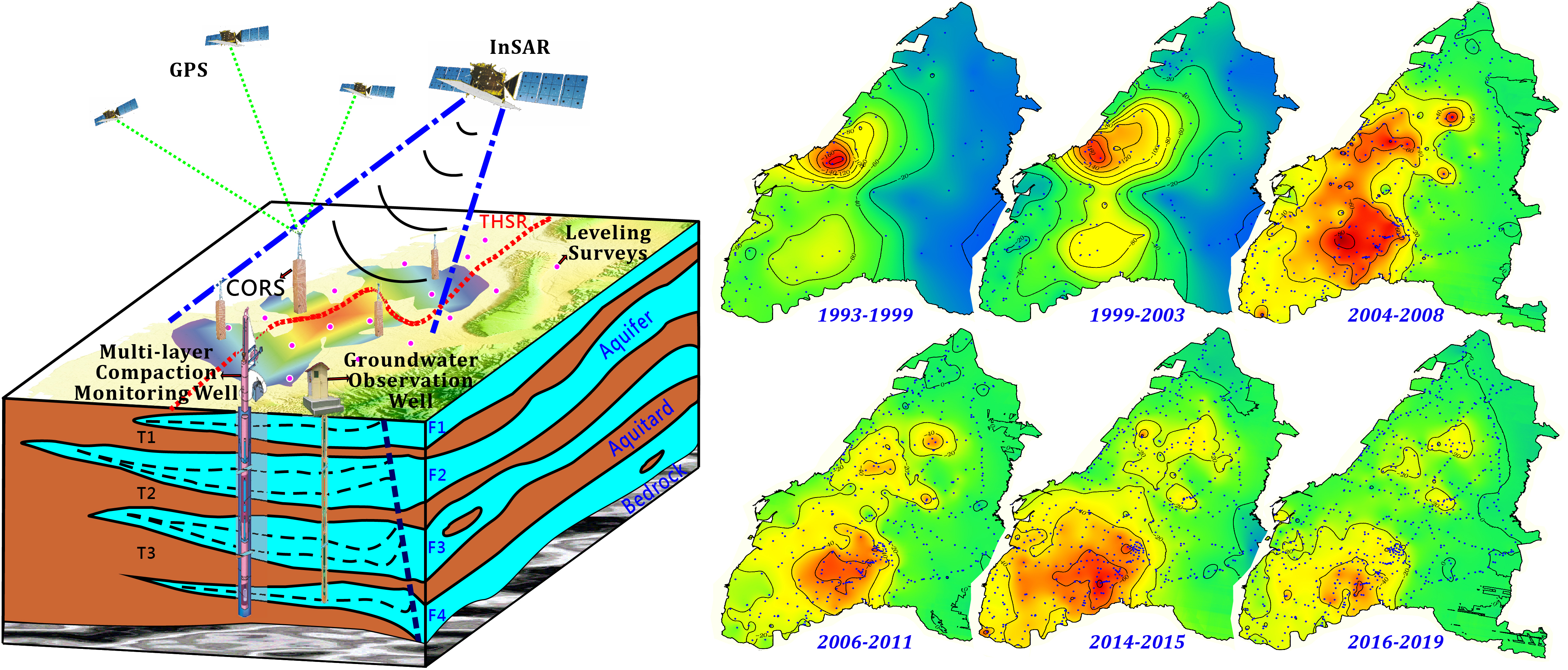
2. Geological Background and Observation Dataset

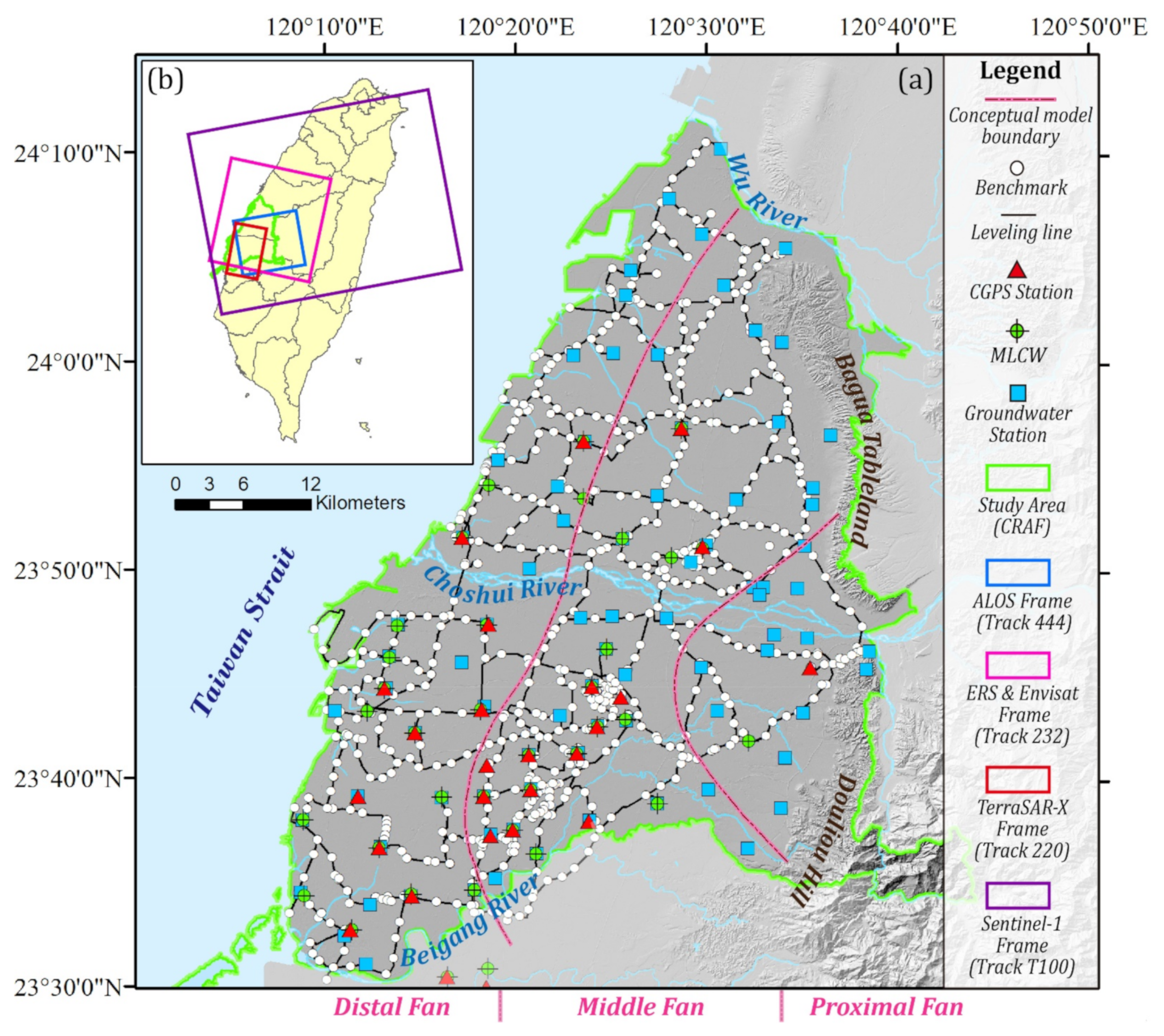
2.1. Geological Background of the Choushui River Alluvial Fan

The CRAF is the most crucial agriculture area in Taiwan, presently encompassing an area of 2079 km2 with elevations between 0 and 100 m (Figure 1a). The CRAF is bordered by the Wu River and Beigang River bounds to the north and the south, with the Bagua-Douliu Hills and the Taiwan Strait to the east and the west. The Choushui River flows through the center of the CRAF and is a border between Changhua and Yunlin counties [29].
Drilling logs data for the CRAF show several unconfined and confined aquifers of Holocene to Pleistocene sediments. The sedimentary layers contain interbedded or lens-structured clay, fine sand, medium fine sand, coarse sand, and gravel separated by impermeable marine mud layers [30]. The complex formations of the CRAF due to frequent sea-level rising and flooding and the channel migration of the Choushui River have divided the CRAF into three geological sections from the inland (east) to the coast (west): the proximal fan, the middle fan, and the distal fan. The sediment thicknesses range from 750 to 3000 m. The grain sizes decrease gradually from the proximal fan to the distal fan [29].
The geological data and the hydrogeology model of the CGS indicate that the CRAF contains four aquifers separated by aquitards at different depths [12]. These aquifers are connected in the proximal fan. The second aquifer spans almost the entire CRAF and is the primary aquifer for withdrawing groundwater because this aquifer has the depth for economic water extraction and is the thickest [29,31,32]. According to previous studies, the middle and the distal fans are covered with more than 250,000 pumping wells, but these two fans are composed of highly compressible materials [33]. As such, over-pumping groundwater there has resulted in groundwater level drops and severe land subsidence.

2.2. Observation Datasets

This section describes the identification of the changing deformation patterns in the CRAF from 1993 to 2019, using long-term multiple-sensor observations, including those from SAR images, CGPS, precise leveling, and MLCWs.

2.2.1. Ground Data

Precise leveling is a method to determine height differences with the precision of millimeter level. In the 1970s, the government of Taiwan started using precise leveling to determine vertical displacements caused by land subsidence in the CRAF. Leveling surveys were carried out along lines forming closed loops of several hundred kilometers in length. The leveling procedure required that the loop misclosure be less than 3 mm√K, where K is the distance between two adjacent benchmarks in km. In some cases, additional leveling surveys within the loops were conducted to increase the local point densities of benchmarks. Measurement errors resulting from the earth’s curvature, atmospheric refraction, and collimation were corrected in the data processing. Based on the records of leveling surveys, the numbers of benchmarks in the CRAF were less than 40 in and before the 1990s, and dramatically increased to more than hundreds since the 2000s [26,34]. In 2019, the total number of benchmarks reached 832, equivalent to a density of 0.4 benchmarks per square kilometer [34].
Tens of CGPS stations have been established in the CRAF. Three-dimensional coordinate components of the CGPS stations provide the mm level and cm level coordinate changes in the horizontal and vertical directions, respectively. However, the displacements at these CGPS stations are not always suitable for validating surface deformations derived by SAR interferometry because some of the GPS records can be short and span irregular periods. Among these CGPS stations located within the SAR image frames, 23 CGPS stations were available for providing reliable, long-term time series measurements. The daily CGPS data were processed with the software Bernese 5.2, and the weekly solution was formed using seven daily network solutions. Accurate and timely GPS satellite ephemerides from the final products of the International GNSS Service (IGS) were also used to reduce the orbit errors. KMNM, located at latitude = 24°27′49″ and longitude = 118°23′18″ in Kinmen, is a station in the IGS network. It was selected as the reference station to constrain the GPS network adjustments. This study used leveling measurements, which are essentially different from GPS data, as well as InSAR data/measurements. The conceptual difference has been clearly described by Wang et al. [35].
An MLCW is a device to measure compactions at different depths with millimeter accuracy [36]. An MLCW is equipped with several magnetic rings anchored at the borders of varying stratum properties in a borehole. The compactions between two neighboring magnetic rings show the deformation in the stratigraphic section. By measuring and analyzing the variations of all installed rings monthly, we can determine the total cumulative compaction from the ground surface to a depth of 300 m.

2.2.2. SAR Data

We determined ground deformations in the CRAF by SBAS InSAR using SAR images from ERS-1/2, Envisat, ALOS, TerraSAR-X, and Sentinel-1 provided by the European Space Agency (ESA), the Japan Aerospace Exploration Agency (JAXA), and the German Aerospace Centre (DLR). Table 1 shows detailed information about these SAR images and selected parameters of the five satellites. Figure 1b shows the distribution of the image frames in the CRAF.

3. Methods

SAR interferometry has been proven to be a powerful and effective geodetic technique for measuring surface deformations, neo-tectonic activities, and natural hazards, such as landslides, with high spatial resolution, sub-centimeter accuracy, and high-cadence observations (~1–2 passes per month) [4,5,16,37,38,39,40]. Nevertheless, the interferometric phase measurements are often affected by the spatial and temporal decorrelation of radar signals, resulting from satellite orbital errors, DEM errors, phase unwrapping errors, and atmospheric artifacts. In some cases, the atmospheric artifacts are the main factor in reducing the accuracy of InSAR measurements and can only be removed with difficulty from SAR interferograms [20,41,42]. Taiwan is situated in a subtropical area, and most parts of the CRAF are covered by dense vegetation and fishponds in the coastal areas. The various surface features and water vapor variations can easily cause spatial decorrelation in conventional InSAR and lead to degraded accuracy in the deformation measurements. In order to overcome the limitations of InSAR technology in the CRAF, the SBAS approach was used in this study.

3.1. Small Baseline Subset Interferometry

An SAR image contains pixels that have an observable phase resulting from the returns of many scatterers on the ground. If these scatterers change with respect to each other along with time, the returned phase signals will vary in a random manner, leading to decorrelations. SBAS exploits selected SAR image pairs separated by short time intervals and small perpendicular baselines to minimize the effects of temporal and spatial decorrelation and maximize the number of distributed scatterers (DSs) detected on the ground [23,43]. The SBAS algorithm used in this study was clearly described by Hooper et al. [22,44] and will not be repeated here.
In this study, the SBAS approach and the three-dimensional spatiotemporal unwrapping were implemented using the StaMPS/MTI software developed by Hooper et al. [22,44]. The digital elevation model from the SRTM mission was resampled on a 25 m grid to estimate the topographic contributions to the observed phases. We used the precise orbits released by the Delft Institute for Earth-Oriented Space Research (DEOS) to reduce the errors in phases caused by the orbit errors of ERS-1/2 and Envisat. In summary, the following procedure was used to process all SAR datasets:
  • ROI_PAC software was used to process the raw SAR images data into single look complex (SLC) images. Then, the SBAS network of interferograms was generated by the Doris and SNAP software packages. In this step, the major orbital and topographic effect was removed;
  • The SBAS approach, implemented by StaMPS/MTI, was used to analyze the interferometric time series and for quality checking and outlier detection. This step resulted in time series of LOS displacements;
  • The LOS displacements at each measurement epoch were interpolated on a 50 m grid to calculate the linear displacement rates.

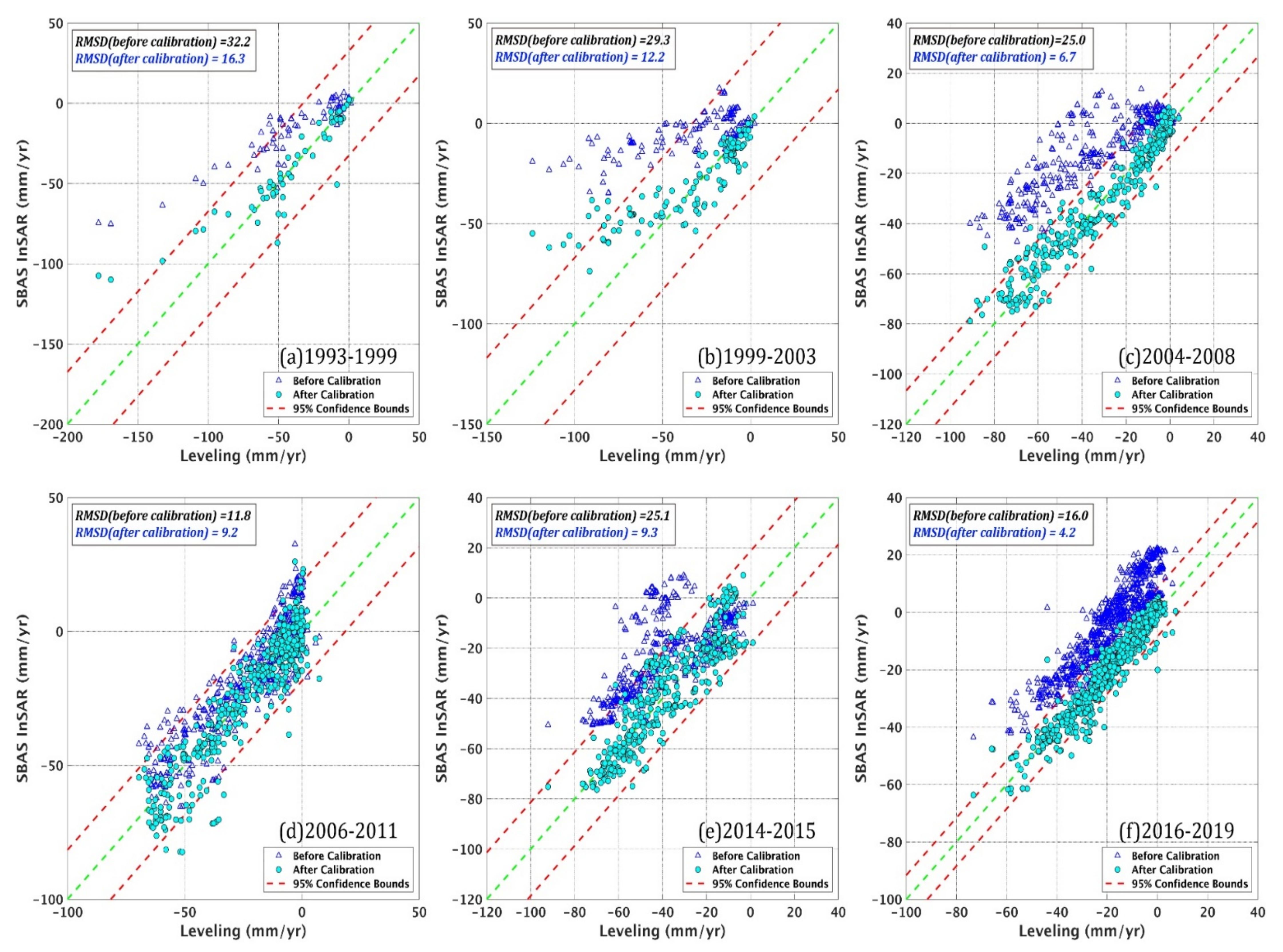
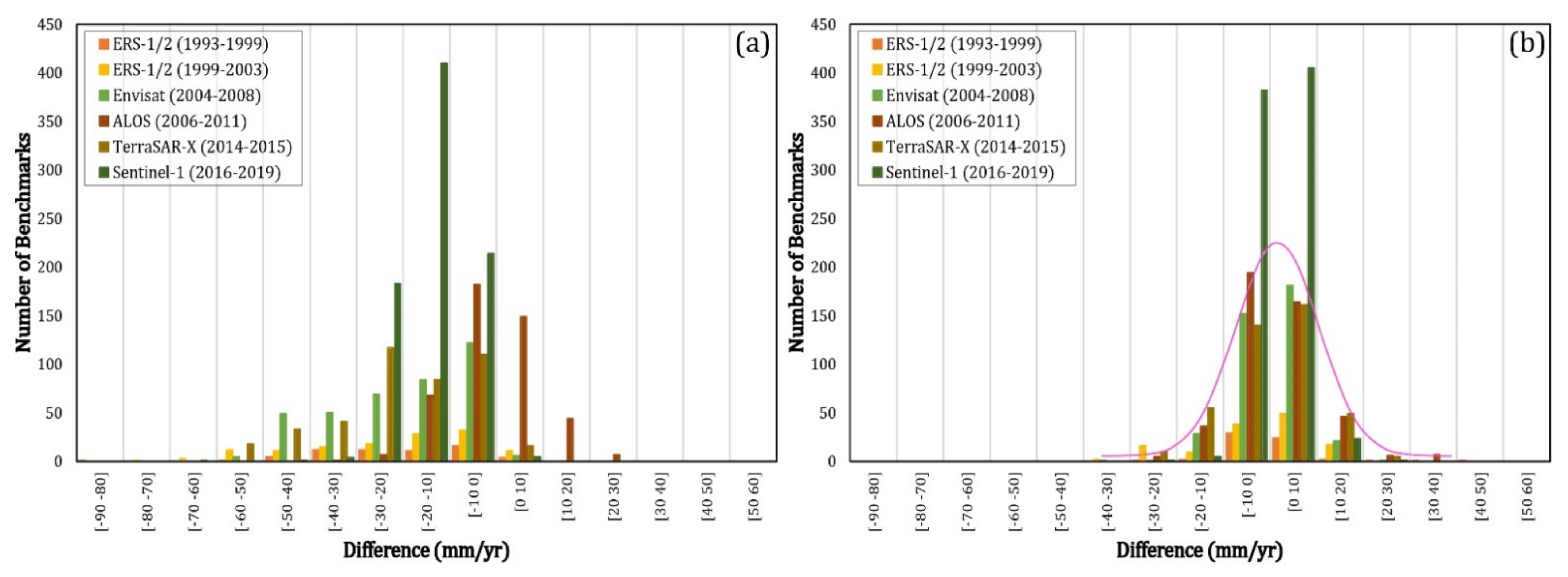
3.2. Calibrating the Initial LOS Velocities from InSAR

Stacks of multiple-source SAR images acquired over the periods 1993–1999, 1999–2003, 2004–2008, 2006–2011, 2014–2015, and 2016–2019 were processed to obtain initial LOS displacement rates, which contain the measuring uncertainty caused by orbit errors, DEM errors, and atmospheric effects, etc. [45,46,47,48,49,50]. However, it is difficult to separate each error source from the SAR dataset. The measuring uncertainty can be modeled by a planar function corresponding to the spatial variation in the interferograms [45,48]. We used the CGPS measurements to find the parameters of the planar function and thereby calibrate the initial deformations from InSAR [46,47,49,50]. This calibration procedure can be summarized as follows.
  • Define a local reference frame based on a reference point located outside the subsiding area. In this study, the stable CGPS station LNJS (the mean velocity of vertical displacement is nearly -5 mm/yr) was chosen as the reference point for comparing InSAR measurements with other geodesy data.
  • Convert the three-dimensional velocity components from CGPS into the LOS velocity (VLOS) with
    V L O S = sin θ sin α   sin θ cos α       cos θ V N V E V h ,
    where VN, VE, and Vh are the velocities in the north, east, and vertical directions and θ and α are the incidence angle and the satellite heading angle (azimuth), respectively.
1.
Calculate the differences between CGPS-derived and InSAR-derived LOS velocities. The differences within a 250 m radius around the CGPS stations can be used to compute the total squared misfit:
R 2 = i = 1 N d i m A + m B x i + m C y i 2 ,
where ∆di is the difference between CGPS and InSAR measurements at station i, xi and yi are the east and north planar coordinates of the i th station, N is the total number of CGPS stations, and mA, mB, and mc are the coefficients of the plane.
2.
Determine mA, mB, and mc by minimizing R2 (the least squares method). The initial LOS velocities were corrected for the velocities determined by the plane.
The horizontal motions of the CRAF are about −3 to 6 mm/yr in the north direction and −7 to 0 mm/yr in the east direction. The horizontal velocity components are relatively small and introduce only small effects on the InSAR-derived LOS velocities. Thus, we assumed that the effect of horizontal motion in the CRAF could be neglected. This assumption has also been adopted in a number of other studies [5,27,50,51,52]. The vertical velocity component derived from a calibrated LOS velocity can be computed as (see Equation (1)):
V h = V L O S / cos θ ,
which is compatible and can be compared with values from precise leveling or GNSS.

4. Results and Discussion

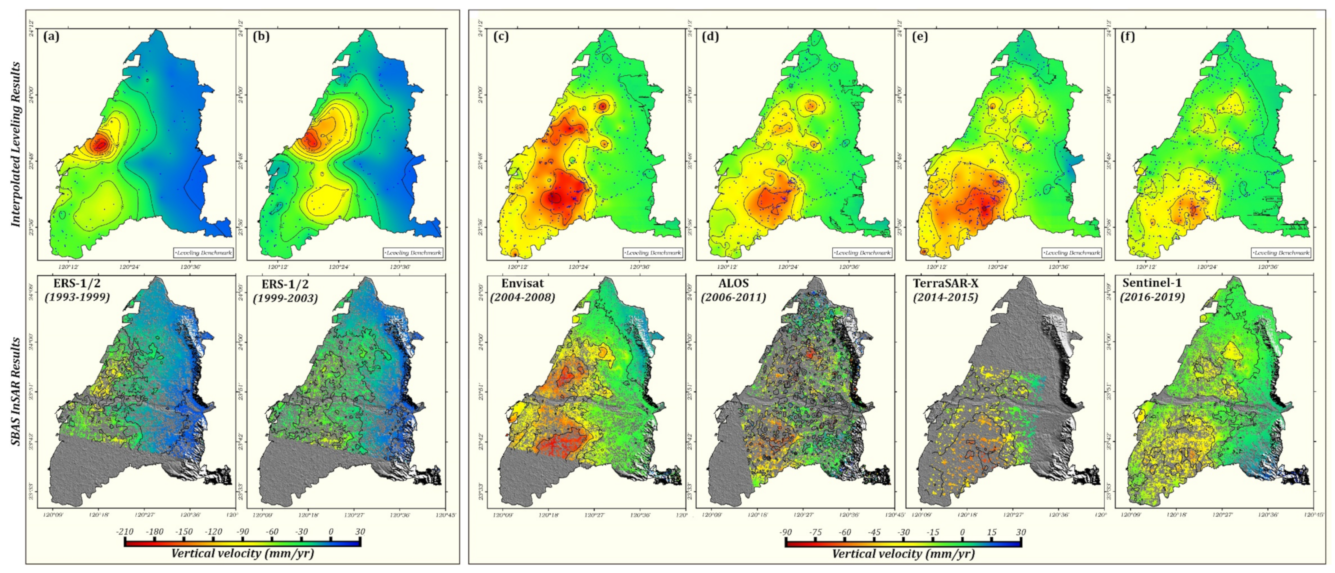
4.1. Vertical Velocities from the Calibrated InSAR Result

For each leveling benchmark, the vertical velocity from the calibrated InSAR-derived LOS velocities averaged over a radius of 250 m around the benchmark was compared with the value from the leveling. Figure 2 shows such comparisons at the benchmarks with leveling measurements commensurate with the InSAR measurements from the five satellite missions (Table 1). The small variances and nearly linear relationships between the two results given in Figure 2 suggest that the SAR images and our processing method were able to measure vertical deformations consistent with those from ground-based sensors such as leveling. The correlation coefficients (r) show that InSAR-derived displacements and leveling observations were highly correlated (r > 0.9) (Table 2). Moreover, the root mean squared (RMS) differences between the InSAR-based and leveling-based velocities ranged from 11.8 to 32.2 mm/yr before the InSAR calibration, decreasing to 4.2–16.3 mm/yr after the calibration. Figure 3 shows the histograms of the leveling–InSAR differences, suggesting that 66.4–96.3% of the differences were within 10 mm/yr after the InSAR calibration. The differences after the calibration (Figure 3b) followed a normal distribution and had a zero mean; this was not the case for the differences without the InSAR calibration (Figure 3a).
However, there were several anomalous vertical velocities from InSAR in the coastal region and regions covered with vegetation and agricultural fields. These anomalous InSAR-derived velocities were lower than the rates from leveling and particularly occurred in the area with higher ground displacements. A similar problem has been reported in several previous studies as well [1,53,54,55]. These anomalies are likely caused by poor phase coherence, phase unwrapping errors, atmospheric effects, large displacement gradients, and inconsistent observation periods between leveling and InSAR.

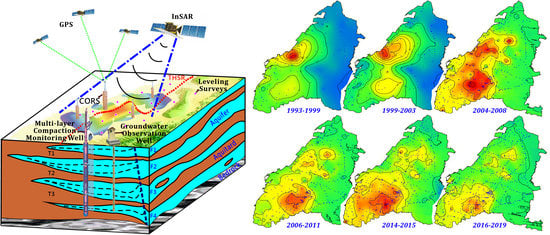
4.2. Space-Time Evolutions of Land Subsidence Values from 1993 to 2019

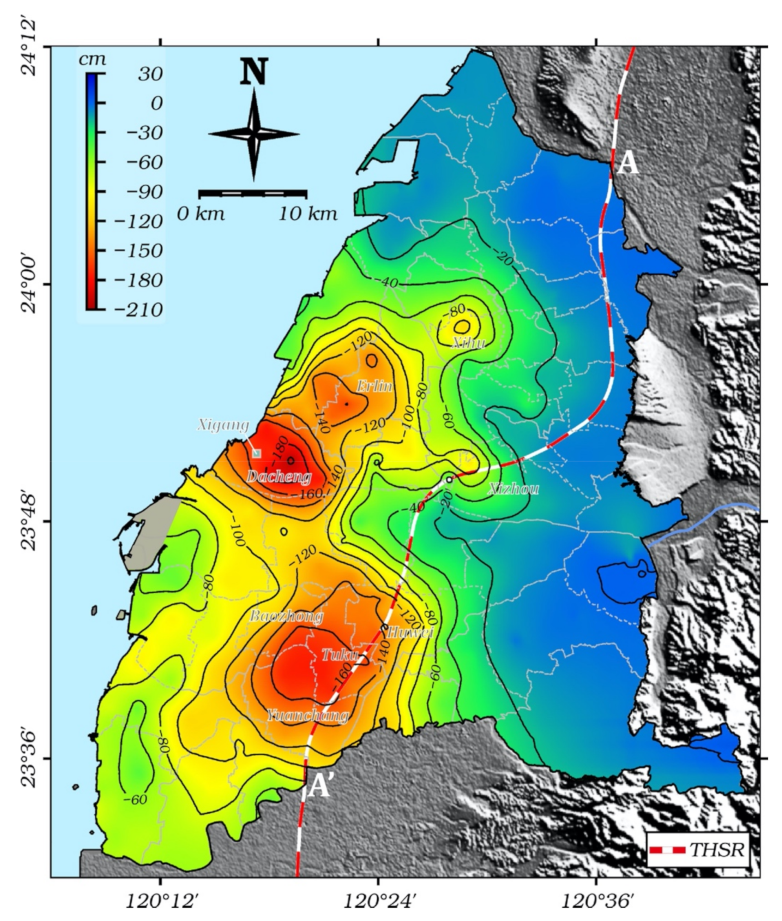
4.2.1. Cumulative Land Subsidence between 1993 and 2019

Figure 4 shows the long-term cumulative land subsidence value from precise leveling results between 1993 and 2019 on a 100 m grid using interpolated leveling measurements obtained through inverse distance weighted interpolation (IDW). The IDW method is commonly used to interpolate scatter points that do not necessarily have a relationship with or influence over neighboring data values and preserve local data variations yielding suitable results [56,57]. Hence, we used a quadratic weighting power within a 2 km radius neighborhood to obtain 100 m regularly spaced grids.
The cumulative subsidence in Figure 4 has two main features. First, a coastal bowl-shaped subsidence center occurred near Dacheng Township of Changhua County, with a maximum subsidence value of 210 cm. Second, several scattered subsidence centers occurred in the inland regions, including Erlin, Xihu, and Xizhou Townships in Changhua County and Huwei, Tuku, and Yuanchang Townships in Yunlin County, with subsidence values ranging from 80 to 180 cm. Taiwan High Speed Rail (THSR), the most important public transportation system in Taiwan, passes through such scattered subsidence centers. The THSR’s safety may be affected by the differential settlements induced by the spatially varying subsidence values along the THSR route here.

4.2.2. Evolutions of Land Subsidence

The short-term average vertical velocities derived from leveling and InSAR are shown in Figure 5. The InSAR results span three decades, i.e., 1993–2003 for ERS-1/2, 2004–2008 for Envisat, 2006–2011 for ALOS, 2014–2015 for TerraSAR-X, and 2016–2019 for Sentinel-1. The InSAR results provided detailed spatial and temporal evolutions of land subsidence in the CRAF.
In the 1990s, the main subsidence areas were located in the coastal region and gradually shifted eastward towards the inland area. The areas with continual deformations were mainly located in the middle and distal fans of the CRAF. The most pronounced deformation pattern was comprised of the several subsidence areas in the middle fan, including the townships of Erlin, Xihu, and Xizhou in Changhua County, and the townships of Huwei, Tuku, Yuanchang, and Baozhong in Yunlin County. Here, the largest subsidence rates exceeded 50 mm/yr. Noticeable subsidence also occurred in some coastal industrial zones, particularly in Yunlin’s offshore industrial park, with a decreasing deformation rate from north to south. These observed subsidence values in the coastal region are probably due to heavy groundwater usage. Figure 5 suggests that the CRAF has experienced land subsidence of varying magnitudes over varying locations. Due to groundwater extraction, land subsidence in the CRAF is still ongoing to date [32], but the rates of subsidence tend to diminish over time.
Figure 5 also indicates that, between 1993 and 2003, large discrepancies between the leveling- and InSAR-derived subsidence rates occurred in the coastal area, particularly discrepancies between the maximum rates from these two sensors. Leveling detected a maximum rate of 200 mm/yr, while the maximum rate from InSAR was only 110 mm/yr. This difference might be attributable to the several factors affecting the InSAR results given in Section 3.2 and the low spatial density of leveling benchmarks. Among the main factors considered should be the sparse temporal sampling during this long period. However, in areas of expected subsidence (based on groundwater extraction and leveling measurements) the subsidence patterns from InSAR were similar to those from leveling, suggesting that InSAR is able to detect vertical motions on the whole.

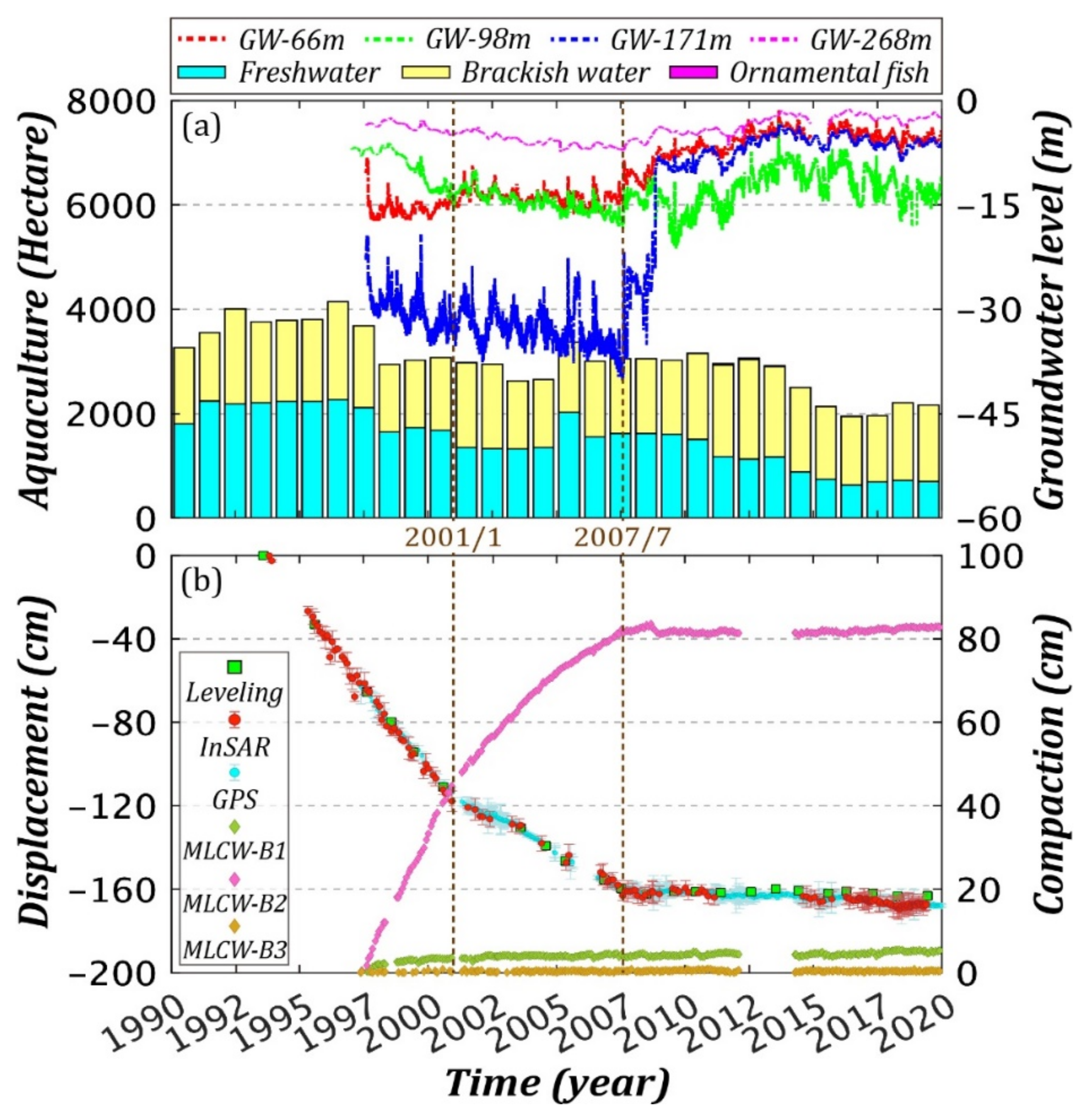
4.3. Analysis of Historical Land Subsidence in Dacheng Township, Changhua

Land use directly affects groundwater quality, recharge rates, and groundwater level variation and is associated with ground subsidence. The coastal lands of Changhua have long been used for freshwater aquaculture that requires groundwater for breeding fish. A dataset provided by the Changhua County government shows that the total area of freshwater aquaculture has been gradually declining and decreased from 4007 ha to 2164 ha between 1992 and 2019 (Figure 6a) [58]. The largest decline occurred in the area with the highest percentage of aquaculture use, from 2300 ha to 700 ha approximately. As a result, the groundwater levels of shallow aquifers increased with time, reducing land subsidence over time.
Figure 6b shows an analysis of the long-term evolution of land subsidence in Dacheng, the township with the largest subsidence rates in Changhua County. The land subsidence values from the ground-based sensors (leveling, GPS, and MLCW) and InSAR are consistent and show a continuous decline from 1993 to 2019. Note that the major compaction in Dacheng occurred in the layers with depths between 52 and 180 m and with materials composed of fine sand and clay, belonging to the B2 layer of the conceptual aquifer model of the CRAF [29].
Land subsidence in Dacheng is largely the result of lowered groundwater level, and surface deformations in Dacheng are highly correlated with the groundwater level fluctuations in the two aquifers underlying the surface of Dacheng. The variations in the displacement pattern of Dacheng suggest that land subsidence in Dacheng has undergone three stages of changes: “before 2001”, “2001–2007”, and “post 2007”.
Before 2001, the maximum annual subsidence rate was detected by leveling and the average subsidence rate in Dacheng was larger than 140 mm/yr. Our data show that the groundwater levels of Xigang station in Dacheng declined continually in this stage. The subsidence rates decreased slightly during the period from 2001 to 2007. The groundwater levels here declined constantly, except the groundwater level at 66 m depth, which showed slight recovery from −15.1 m to −12.3 m during this period. After 2007, the groundwater levels at Xigang underwent both seasonal variations and a long-term rising trend. After 2007, groundwater levels at Xigang at 171 m depth dramatically increased, resulting in apparently decreasing compactions with occasional rebounds. However, current data show that the land subsidence rate in Dacheng is still ongoing but is decreasing. Recent maximum subsidence rates in Dacheng are below 10 mm/yr.

4.4. Land Subsidence Analysis along the THSR in the CRAF

The THSR uses viaducts for its rails in the middle to south section. More than 20,000 columns have been installed to support the viaducts in the section. In general, the columns are 1.5–2.5 m in diameter and 35–72 m in length [59]. As a consequence of the land subsidence in this section, the bearing capacity of the columns is reduced by negative frictional forces. According to the design standards for Japanese National Railways, the effect of negative frictional forces should be considered in the design of the foundation columns if the annual subsidence exceeds 2 cm. If the annual subsidence is over 4 cm, negative frictional forces should be fully assessed. The THSR passes through the CRAF and has a section with the largest subsidence rates exceeding 4 cm/yr.
Figure 7 shows the land subsidence rates along a section (A-A’) of the THSR in the CRAF from the multiple SAR datasets, which indicated subsidence of similar patterns and magnitudes. Apparent spatially varying subsidence rates occurred around the THSR sections over Xizhou (zone 1), Huwei–Tuku (zone 2), and Tuku–Yuanchang (zone 3). From Xizhou Township toward the south, the subsidence rates increased significantly until the Yunlin THSR station in Huwei, where the rates started to decline. A newly formed subsidence center between Tuku and Yuanchang (zone 3) that occurred in 2014 was detected by InSAR. Zone 3 experienced high subsidence rates ranging from 60 to 70 mm/yr between 2014 and 2015, but the rates declined to between 30 and 50 mm/yr from 2016 to 2019. Figure 8 shows the MLCW measurements at STES near the subsidence center of zone 3 which suggested that the major compaction occurred at the depth of 50 m, followed by the minor compaction at depths of 50–200 m. The layer that suffered the major compaction is composed of coarse sand, fine sand, silt, and clay, which are susceptible to compressions. We found that extensive groundwater pumping in the depths of 20–40 m contributed to the major compaction seen in Figure 8.
It has been shown that land subsidence can also cause lateral (horizontal) displacements. For example, Bawden et al. [60] used an elastic model to simulate the response of an elastic material to aquifer pumping or recharge, and showed that the largest horizontal displacement (about 1/3 of the largest displacement) occurs near the margins of the subsidence. Hence, we recommend that both the vertical and lateral movements caused by land subsidence should be considered when assessing the risk of land subsidence to railway safety.

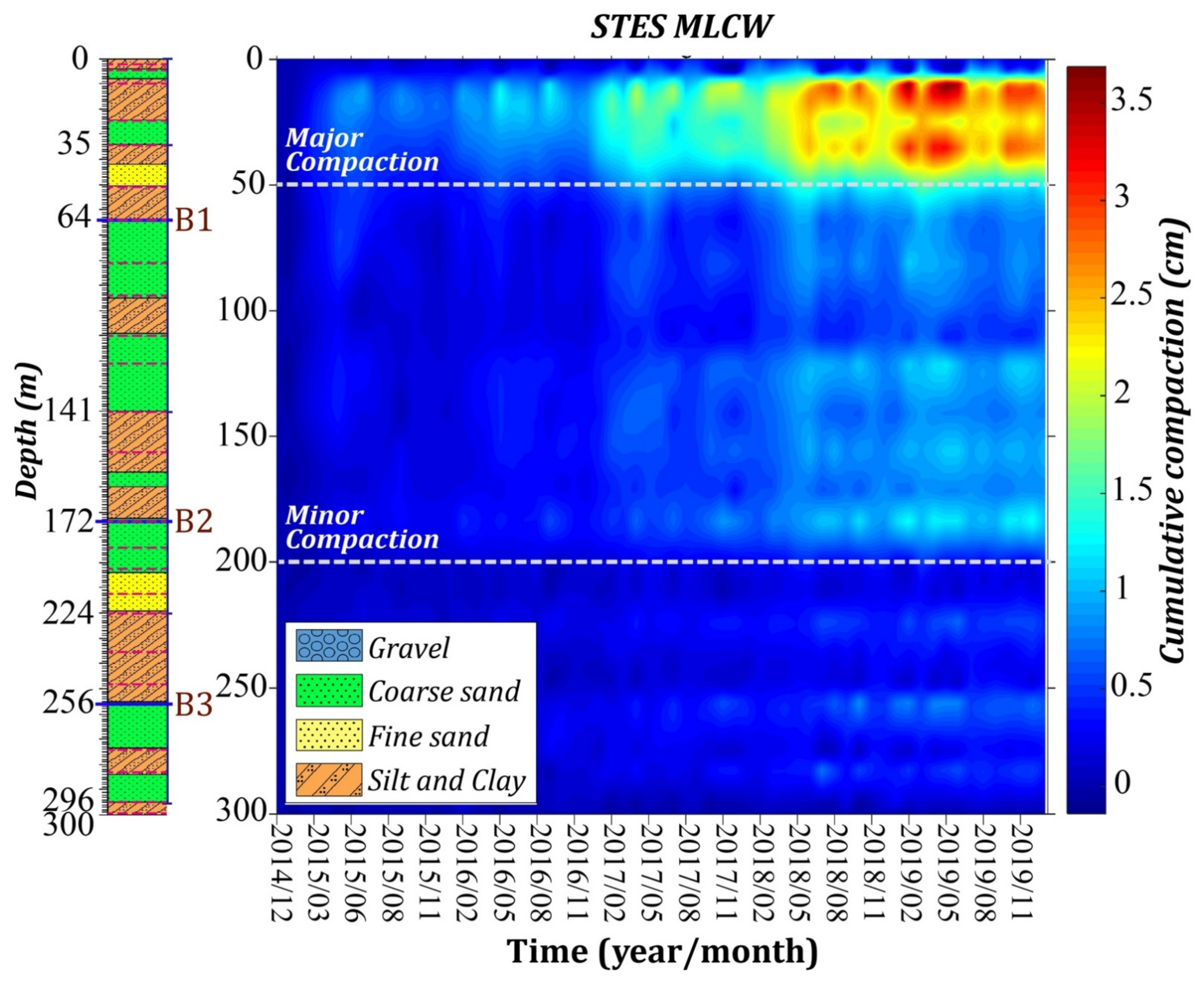
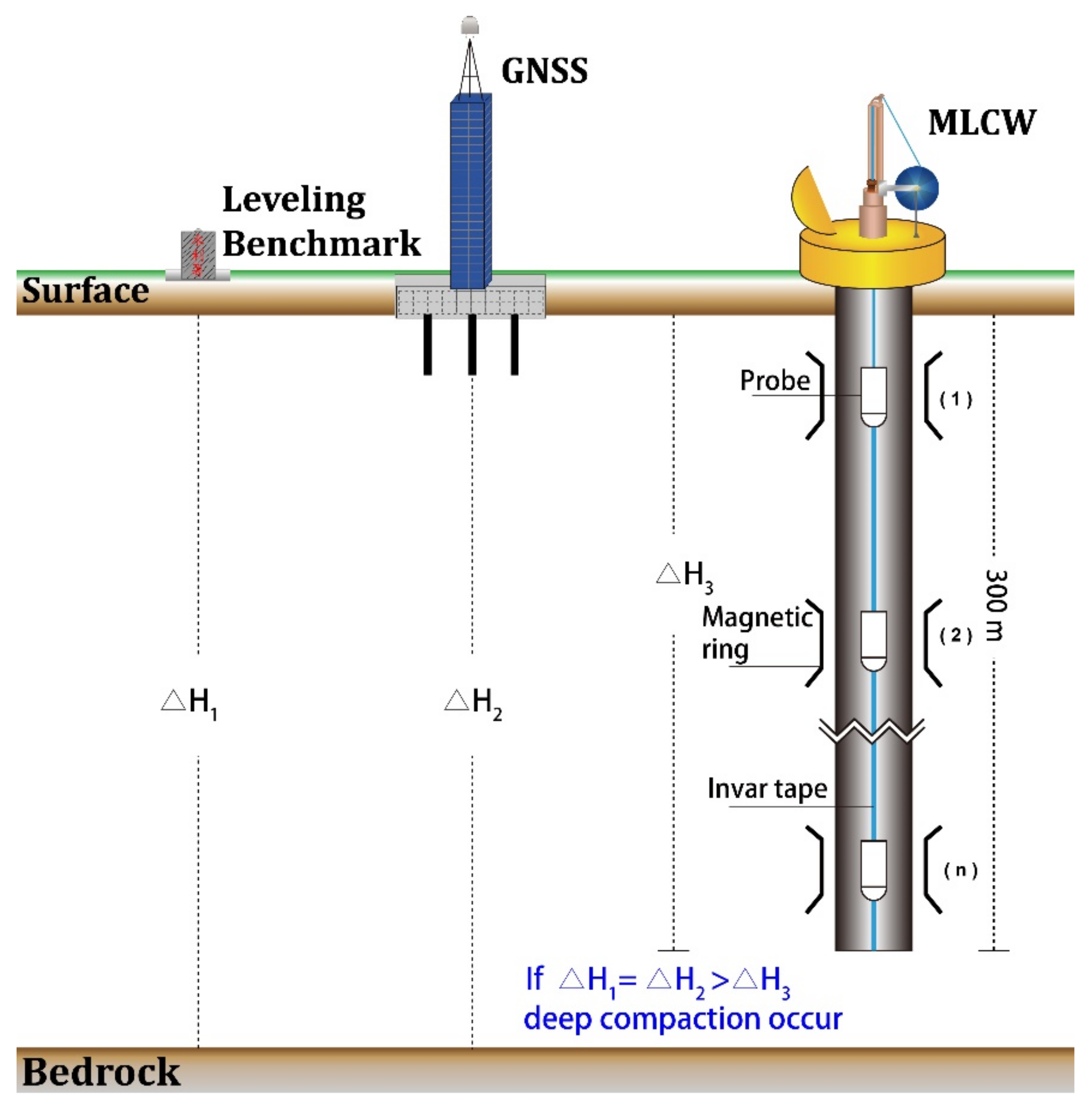
4.5. Distribution of the Deep Compactions

In general, compactions measured by leveling (∆H1) and GPS (∆H2) represent the vertical deformations between the ground surface and the bedrock, but compactions measured by MLCWs (∆H3) in this study represent only compactions from the ground surface to 300 m depth. This is illustrated in Figure 9. If ∆H1 = ∆H2 = ∆H3, there is no compaction below 300 m. However, if ∆H1 = ∆H2 > ∆H3, then the leveling and GPS measurements indicate compactions below 300 m, defined as deep compactions. Linear regression analysis can be applied to obtain the average velocity of both leveling (Vl) and MLCW (Vm) datasets. Hence, the deeper compaction rate (Vd = Vl − Vm), i.e., the deformation generated between the depth of 300 m and the bedrock, can be calculated under this assumption. We computed the vertical velocities from the leveling and MLCW measurements in the CRAF at the stations with both measurements, allowing us to examine deep compactions in the CRAF.
In response to the call for a “Concrete Solution for the Long-Term Land Subsidence in Yunlin–Changhua Area” initiated in 2011, in this study we mapped the deep compactions in the CRAF over two periods, i.e., 2006–2010 and 2011–2019. The mapped deep compactions are shown in Figure 10. From 2006 to 2010, deep compactions greater than 20 mm/yr were detected in the middle fan, including Xizhou Township and Tuku Township. The townships of Erlin, Huwei, and Yuanchang also experienced deep compactions, with smaller rates of 10–20 mm/yr. Some areas other than these townships suffered minor deep compactions (rates < 10 mm/yr). Deep compactions in these regions were persistent, but the rates decreased from 2011 to 2019. After 2019, the rates of deep compaction in Xizhou and Tuku were only 10 to 20 mm/yr. Our observations also indicated reduced rates at 0–10 mm/yr in Huwei and Yuanchang.
Figure 11 shows changes in groundwater level from April 2011 to April 2019 in aquifers 3 and 4 in the CRAF. Positive changes in aquifers 3 and 4 indicated reduced groundwater pumping, which occurred in Tuku and Yuanchang (middle fan of the CRAF). Here the increases of the groundwater levels ranged from 1 to 3 m in aquifer 3 and from 0 to 1.5 m in aquifer 4, respectively.
The reductions in deep compactions were due to the de-commissions of the deep wells responsible for the deep compactions. According to the surveying reports of the Ministry of Economic Affairs, more than one thousand pumping wells in the CRAF have been decommissioned, resulting in reduced groundwater pumping of approximately 44.3 million tons between 2011 to 2019 [34]. The overall groundwater levels in Xizhou, Huwei, Tuku, and Yuanchang rose obviously since this measure (de-commissioning wells) took effect in 2011. In summary, reducing deep compactions in the CRAF requires effective management of groundwater pumping wells.

5. Conclusions

This study used multiple-sensor observations to show the spatial and temporal variations of land subsidence in the CRAF from 1993 to 2019. We used the CGPS observations to calibrate the SBAS InSAR measurements effectively. Our assessments showed that the vertical deformations from leveling and InSAR were consistent, despite some large discrepancies that were explained in earlier sections.
A maximum cumulative subsidence of 210 cm occurred in Dacheng from 1993 to 2019. The changes in the coastal areas for freshwater aquaculture affect the magnitudes of land subsidence in Changhua, especially in Dacheng. Persistent land subsidence in the inland area of the CRAF was detected by our observations, but the rates of subsidence declined from 2004 to 2019. Several subsidence bowls were identified in Erlin, Xihu, and Xizhou in Changhua County, as well as in Huwei, Tuku, Yuanchang, and Baozhong in Yunlin County. A newly formed subsidence center was also detected between Tuku and Yuanchang; the THSR passed through this section. The distribution of deep compactions was mapped for the first time using the differences between the subsidence rates from leveling and MLCWs. Before 2011, Xizhou and Tuku suffered the largest deep compactions, with rates exceeding 20 mm/yr. From 2011 to 2019, groundwater levels here rebounded to reduce the deep compactions.
Land subsidence can be caused by natural and human-induced factors, each having different contributions. One natural cause is the geological influence that has lasted thousand years and contributed only 0.6 to 2.1 mm/yr to the total land subsidence in the CRAF [61]. The major causes of land subsidence in the CRAF are manmade and are largely due to over-pumping groundwater. Therefore, a proper management scheme of groundwater resources is the key to reducing and preventing land subsidence. A good scheme should also take into account local societal needs and local cultures in order for the scheme to be long-lasting and supported by locals.

Author Contributions

Conceptualization, Y.-A.C., C.-P.C. and W.-C.H.; formal analysis, Y.-A.C., C.-P.C., C.H. and J.-Y.Y.; investigation, Y.-A.C. and W.-C.H.; resources, C.-P.C. and W.-C.H.; writing—original draft preparation, Y.-A.C.; writing—review and editing, all; visualization, Y.-A.C. and C.-H.L.; supervision, C.-P.C. All authors have read and agreed to the published version of the manuscript.

Funding

This research received no external funding.

Acknowledgments

The authors thank the Water Resource Agency, Department of Economics, Taiwan, for providing the leveling, CGPS, MLCW, and GW data. We also thank the ESA and JAXA for providing the ERS-1/2, Envisat, Sentinel-1, and ALOS SAR data through projects C1P.14092 and PI-1380, respectively. This study was partially supported by MOST/Taiwan, under grant numbers (C.-P.C.) and 110-MOEA-M-008-001 from 2020 to 2021.

Conflicts of Interest

The authors declare no conflict of interest.

References

  1. Amelung, F.; Galloway, D.L.; Bell, J.W.; Zebker, H.A.; Laczniak, R.J. Sensing the ups and downs of Las Vegas: InSAR reveals structural control of land subsidence and aquifer-system deformation. Geology 1999, 27, 483–486. [Google Scholar] [CrossRef]
  2. Castellazzi, P.; Garfias, J.; Martel, R.; Brouard, C.; Rivera, A. InSAR to support sustainable urbanization over compacting aquifers: The case of Toluca Valley, Mexico. Int. J. Appl. Earth Obs. Geoinf. 2017, 63, 33–44. [Google Scholar] [CrossRef]
  3. Herrera-García, G.; Ezquerro, P.; Tomás, R.; Béjar-Pizarro, M.; López-Vinielles, J.; Rossi, M.; Mateos, R.M.; Carreón-Freyre, D.; Lambert, J.; Teatini, P.; et al. Mapping the global threat of land subsidence. Science 2021, 371, 34–36. [Google Scholar] [CrossRef]
  4. Hung, W.-C.; Hwang, C.; Chang, C.-P.; Yen, J.-Y.; Liu, C.-H.; Yang, W.-H. Monitoring severe aquifer-system compaction and land subsidence in Taiwan using multiple sensors: Yunlin, the southern Choushui River Alluvial Fan. Environ. Geol. 2010, 59, 1535–1548. [Google Scholar] [CrossRef]
  5. Hung, W.-C.; Hwang, C.; Chen, Y.-A.; Chang, C.-P.; Yen, J.-Y.; Hooper, A.; Yang, C.-Y. Surface deformation from persistent scatterers SAR interferometry and fusion with leveling data: A case study over the Choushui River Alluvial Fan, Taiwan. Remote Sens. Environ. 2011, 115, 957–967. [Google Scholar] [CrossRef]
  6. Lanari, R.; Lundgren, P.; Manzo, M.; Casu, F. Satellite radar interferometry time series analysis of surface deformation for Los Angeles, California. Geophys. Res. Lett. 2004, 31, 1–5. [Google Scholar] [CrossRef]
  7. Normand, J.C.L.; Heggy, E. InSAR assessment of surface deformations in urban coastal terrains associated with groundwater dynamics. IEEE Trans. Geosci. Remote. Sens. 2015, 53, 6356–6371. [Google Scholar] [CrossRef]
  8. Chen, C.-H.; Wang, C.-H.; Hsu, Y.-J.; Yu, S.-B.; Kuo, L.-C. Correlation between groundwater level and altitude variations in land subsidence area of the Choshuichi Alluvial Fan, Taiwan. Eng. Geol. 2010, 115, 122–131. [Google Scholar] [CrossRef]
  9. Fan, K.-L. The Coastal Environmental Characteristics of Taiwan. Chem. Ecol. 1995, 10, 157–166. [Google Scholar] [CrossRef]
  10. Hsu, S.-K. Plan for a groundwater monitoring network in Taiwan. Hydrogeol. J. 1998, 6, 405–415. [Google Scholar] [CrossRef]
  11. Liu, C.-H.; Huang, C.-T. Taiwan land subsidence caused by groundwater over drafting. J. Civ. Hydraul. Eng. 2002, 29, 47–57. [Google Scholar]
  12. Wang, C.H.; Peng, T.R.; Liu, T.K. The salinization of groundwater in the northern Lan-Yang Plain, Taiwan: Stable isotope evidence. J. Geol. Soc. China 1996, 39, 627–636. [Google Scholar]
  13. Wang, C.H.; Kuo, C.H.; Peng, T.R.; Chen, W.F.; Liu, T.K.; Chiang, C.J. Isotope characteristics of groundwaters in the Pingtung Plain, southern Taiwan. W. Pac. Earth Sci. 2003, 3, 1–8. [Google Scholar]
  14. Bell, J.W.; Amelung, F.; Ferretti, A.; Bianchi, M.; Novali, F. Permanent scatterer InSAR reveals seasonal and long-term aquifer-system response to groundwater pumping and artificial recharge. Water Resour. Res. 2008, 44. [Google Scholar] [CrossRef] [Green Version]
  15. Castellazzi, P.; Longuevergne, L.; Martel, R.; Rivera, A.; Brouard, C.; Chaussard, E. Quantitative mapping of groundwater depletion at the water management scale using a combined GRACE/InSAR approach. Remote Sens. Environ. 2018, 205, 408–418. [Google Scholar] [CrossRef]
  16. Chang, C.P.; Chang, T.Y.; Wang, C.T.; Kuo, C.H.; Chen, K.S. Land-surface deformation corresponding to seasonal ground-water fluctuation, determining by SAR interferometry in the SW Taiwan. Math. Comput. Simul. 2004, 67, 351–359. [Google Scholar] [CrossRef]
  17. Hoffmann, J.; Zebker, H.A.; Galloway, D.L.; Amelung, F. Seasonal subsidence and rebound in Las Vegas Valley, Nevada, observed by synthetic aperture radar interferometry. Water Resour. Res. 2001, 37, 1551–1566. [Google Scholar] [CrossRef]
  18. Ojha, C.; Shirzaei, M.; Werth, S.; Argus, D.F.; Farr, T.G. Sustained groundwater loss in California’s central Valley exacerbated by intense drought periods. Water Resour. Res. 2018, 54, 4449–4460. [Google Scholar] [CrossRef]
  19. Riel, B.; Simons, M.; Ponti, D.; Agram, P.; Jolivet, R. Quantifying ground deformation in the Los Angeles and Santa Ana coastal basins due to groundwater withdrawal. Water Resour. Res. 2018, 54, 3557–3582. [Google Scholar] [CrossRef] [Green Version]
  20. Ferretti, A.; Prati, C.; Rocca, F. Nonlinear subsidence rate estimation using Permanent Scatterers in differential SAR interferometry. IEEE Trans. Geosci. Remote Sens. 2000, 38, 2202–2212. [Google Scholar] [CrossRef] [Green Version]
  21. Ferretti, A.; Prati, C.; Rocca, F. Permanent scatterers in SAR interferometry. IEEE Trans. Geosci. Remote Sens. 2001, 39, 8–20. [Google Scholar] [CrossRef]
  22. Hooper, A. A multi-temporal InSAR method incorporating both persistent scatterer and small baseline approaches. Geophys. Res. Lett. 2008, 35. [Google Scholar] [CrossRef] [Green Version]
  23. Berardino, P.; Fornaro, G.; Lanari, R.; Sansosti, E. A new algorithm for surface deformation monitoring based on small baseline differential SAR interferograms. IEEE Trans Geosci. Remote Sens. 2002, 40, 2375–2383. [Google Scholar] [CrossRef] [Green Version]
  24. Usai, S. A least squares database approach for SAR interferometric data. IEEE Trans. Geosci. Remote Sens. 2003, 41, 753–760. [Google Scholar] [CrossRef] [Green Version]
  25. Tung, H.; Hu, J.-C. Assessments of serious anthropogenic land subsidence in Yunlin County of central Taiwan from 1996 to 1999 by Persistent Scatterers InSAR. Tectonophysics 2012, 578, 126–135. [Google Scholar] [CrossRef]
  26. Lu, C.-H.; Ni, C.-F.; Chang, C.-P.; Chen, Y.-A.; Yen, J.-Y. Geostatistical Data Fusion of Multiple Type Observations to Improve Land Subsidence Monitoring Resolution in the Choushui River Fluvial Plain, Taiwan. Terr. Atmos. Ocean. Sci. 2016, 27, 505–520. [Google Scholar] [CrossRef] [Green Version]
  27. Yang, Y.-J.; Hung, W.-C.; Hwang, C.-W.; Fuhrmann, T.; Chen, Y.-A.; Wei, S.-H. Surface Deformation from Sentinel-1A InSAR: Relation to Seasonal Groundwater Extraction and Rainfall in Central Taiwan. Remote Sens. 2019, 11, 2817. [Google Scholar] [CrossRef] [Green Version]
  28. Lu, C.-Y.; Hu, J.-C.; Chan, Y.-C.; Su, Y.-F.; Chang, C.-H. The Relationship between Surface Displacement and Groundwater Level Change and Its Hydrogeological Implications in an Alluvial Fan: Case Study of the Choshui River, Taiwan. Remote Sens. 2020, 12, 3315. [Google Scholar] [CrossRef]
  29. Central Geological Survey (CGS). The Investigation of Hydrogeology in the Choushui River Alluvial Fan, Taiwan; Central Geological Survey of Taiwan: Taipei, Taiwan, 1999. (In Chinese) [Google Scholar]
  30. Water Conservancy Agency (WCA). Preliminary Analyses of Groundwater Hydrology in the Choshui Alluvial Fan. Groundwater Monitoring Network Program Phase I; Ministry of Economic Affairs: Taipei, Taiwan, 1997. (In Chinese) [Google Scholar]
  31. Liu, C.-W.; Lin, W.-S.; Shang, C.; Liu, S.-H. The effect of clay dehydration on land subsidence in the Yun-Lin coastal area, Taiwan. Environ. Geol. 2001, 40, 518–527. [Google Scholar] [CrossRef]
  32. Liu, C.-H.; Pan, Y.-W.; Liao, J.-J.; Huang, C.-T.; Ouyang, S. Characterization of land subsidence in the Choshui River alluvial fan, Taiwan. Environ. Geol. 2004, 45, 1154–1166. [Google Scholar] [CrossRef]
  33. Water Resources Agency (WRA). Report of the Monitoring, Investigating and Analyzing of Land Subsidence in Taiwan (1/4); Ministry of Economic Affairs: Taipei, Taiwan, 2001. (In Chinese) [Google Scholar]
  34. Water Resources Agency (WRA). Monitoring and Analyzing Land Subsidence of Changhua and Yunlin Area in 2016–2020; Ministry of Economic Affairs: Taipei, Taiwan, 2016–2020. (In Chinese) [Google Scholar]
  35. Wang, G.; Soler, T. Measuring land subsidence using GPS: Ellipsoid height versus orthometric height. J. Surv. Eng. 2015, 141, 05014004. [Google Scholar] [CrossRef]
  36. Hung, W.C.; Hwang, C.; Sneed, M.; Chen, Y.A.; Chu, C.H.; Lin, S.H. Measuring and Interpreting Multilayer Aquifer-System Compactions for a Sustainable Groundwater-System Development. Water Resour. Res. 2021, 57, 1–19. [Google Scholar] [CrossRef]
  37. Castellazzi, P.; Martel, R.; Galloway, D.L.; Longuevergne, L.; Rivera, A. Assessing Groundwater Depletion and Dynamics Using GRACE and InSAR: Potential and Limitations. Groundwater 2016, 54, 768–780. [Google Scholar] [CrossRef] [PubMed] [Green Version]
  38. Chang, C.-P.; Yen, J.-Y.; Hooper, A.; Chou, F.-M.; Chen, Y.-A.; Hou, C.-S.; Hung, W.-C.; Lin, M.-S. Monitoring of surface deformation in Northern Taiwan using DInSAR and PSInSAR techniques. Terr. Atmos. Ocean. Sci. 2010, 21, 447–461. [Google Scholar] [CrossRef] [Green Version]
  39. Massonnet, D.; Feigl, K.L. Radar interferometry and its application to changes in the Earth’s surface. Rev. Geophys. 1998, 36, 441–500. [Google Scholar] [CrossRef] [Green Version]
  40. Yen, J.-Y.; Lu, C.-H.; Chang, C.-P.; Hooper, A.J.; Chang, Y.-H.; Liang, W.-T.; Chang, T.-Y.; Lin, M.-S.; Chen, K.-S. Investigating active deformation in the northern Longitudinal Valley and City of Hualien in eastern Taiwan using Persistent Scatterer and Small-Baseline SAR Interferometry. Terr. Atmos. Ocean. Sci. 2011, 22, 291–304. [Google Scholar] [CrossRef] [Green Version]
  41. Pathier, E. Apports de L’interferometrie Radar Differentielle a L’etude de la Tectonique Active de Taiwan. Ph.D. Thesis, Universite Marne-La-Vallee, Paris, France, 2003; 273p. [Google Scholar]
  42. Zebker, H.A.; Rosen, P.A.; Hensley, S. Atmospheric effects in interferometric synthetic aperture radar surface deformation and topographic maps. J. Geophys. Res. Solid Earth 1997, 102, 7547–7563. [Google Scholar] [CrossRef]
  43. Hooper, A.; Zebker, H.; Segall, P.; Kampes, B. A new method for measuring deformation on volcanoes and other natural terrains using InSAR persistent scatterers. Geophys. Res. Lett. 2004, 31. [Google Scholar] [CrossRef]
  44. Hooper, A.; Segall, P.; Zebker, H. Persistent scatterer interferometric synthetic aperture radar for crustal deformation analysis, with application to Volcán Alcedo, Galápagos. J. Geophys. Res. Atmos. 2007, 112. [Google Scholar] [CrossRef] [Green Version]
  45. Bähr, H.; Hanssen, R.F. Reliable estimation of orbit errors in spaceborne SAR interferometry. J. Geod. 2012, 86, 1147–1164. [Google Scholar] [CrossRef] [Green Version]
  46. Da Lio, C.; Teatini, P.; Strozzi, T.; Tosi, L. Understanding land subsidence in salt marshes of the Venice Lagoon from SAR Interferometry and ground-based investigations. Remote Sens. Environ. 2018, 205, 56–70. [Google Scholar] [CrossRef]
  47. Fuhrmann, T.; Garthwaite, M.C. Resolving Three-Dimensional Surface Motion with InSAR: Constraints from Multi-Geometry Data Fusion. Remote Sens. 2019, 11, 241. [Google Scholar] [CrossRef] [Green Version]
  48. Hanssen, R.F. Radar Interferometry Data Interpretation and Error Analysis; Springer: Dordrecht, The Netherlands, 2001. [Google Scholar] [CrossRef] [Green Version]
  49. Tosi, L.; Strozzi, T.; Da Lio, C.; Teatini, P. Regional and local land subsidence at the Venice coastland by TerraSAR-X PSI. Proc. IAHS 2015, 372, 199–205. [Google Scholar] [CrossRef] [Green Version]
  50. Tosi, L.; Da Lio, C.; Teatini, P.; Strozzi, T. Land Subsidence in Coastal Environments: Knowledge Advance in the Venice Coastland by TerraSAR-X PSI. Remote Sens. 2018, 10, 1191. [Google Scholar] [CrossRef] [Green Version]
  51. Galloway, D.L.; Hudnut, K.W.; Ingebritsen, S.E.; Phillips, S.P.; Peltzer, G.; Rogez, F.; Rosen, P.A. Detection of aquifer system compaction and land subsidence using interferometric synthetic aperture radar, Antelope valley, Mojave Desert, California. Water Resour. Res. 1998, 34, 2573–2585. [Google Scholar] [CrossRef]
  52. Schmidt, D.A.; Bürgmann, R. Time-dependent land uplift and subsidence in the Santa Clara valley, California, from a large interferometric synthetic aperture radar data set. J. Geophys. Res. Solid Earth 2003, 108, 2416–2428. [Google Scholar] [CrossRef] [Green Version]
  53. Huang, M.-H.; Bürgmann, R.; Hu, J.-C. Fifteen years of surface deformation in Western Taiwan: Insight from SAR interferometry. Tectonophysics 2016, 692, 252–264. [Google Scholar] [CrossRef] [Green Version]
  54. Raucoules, D.; Bourgine, B.; de Michele, M.; Le Cozannet, G.; Closset, L.; Bremmer, C.; Veldkamp, H.; Tragheim, D.; Bateson, L.; Crosetto, M.; et al. Validation and intercomparison of Persistent Scatterers Interferometry: PSIC4 project results. J. Appl. Geophys. 2009, 68, 335–347. [Google Scholar] [CrossRef] [Green Version]
  55. Wasowski, J.; Bovenga, F. Investigating landslides and unstable slopes with satellite Multi Temporal Interferometry: Current issues and future perspectives. Eng. Geol. 2014, 174, 103–138. [Google Scholar] [CrossRef]
  56. Haber, J.; Zeilfelder, F.; Davydov, O.; Seidel, H.P. Smooth approximation and rendering of large scattered data sets. In Proceedings of the IEEE Visualization, San Diego, CA, USA, 21–26 October 2001; pp. 341–347. [Google Scholar] [CrossRef] [Green Version]
  57. Mueller, T.G.; Pusuluri, N.B.; Mathias, K.K.; Cornelius, P.L.; Barnhisel, R.I.; Shearer, S.A. Map quality for ordinary kriging and inverse distance weighted interpolation. Soil Sci. Soc. Am. J. 2004, 68, 2042–2047. [Google Scholar] [CrossRef]
  58. Changhua County Government (CCG). The Statistical Yearbook of Changhua County; Changhua County Government: Changhua, Taiwan, 1990–2020. (In Chinese) [Google Scholar]
  59. Seah, T.H.; Moh, Z.C.; Chin, C.T.; Duann, S.W. Pile foundations of Taiwan High Speed Rail. In Proceedings of the 16th International Conference on Soil Mechanics and Geotechnical Engineering, Osaka, Japan, 12–16 September 2005. [Google Scholar] [CrossRef]
  60. Bawden, G.W.; Thatcher, W.; Stein, R.S.; Hudnut, K.W.; Peltzer, G. Tectonic contraction across Los Angeles after removal of groundwater pumping effects. Nature 2001, 412, 812–815. [Google Scholar] [CrossRef]
  61. Chiang, C.J.; Lin, Y.C.; Chen, C.L.; Lai, T.H. Natural and Man-Induced Land Subsidence in the Choushuichi Groundwater Basin. Spec. Publ. Cent. Geol. Surv. 2014, 27, 1–12. (In Chinese) [Google Scholar]
Figure 1. (a) The geographical location of the CRAF and the distribution of the monitoring instruments. White dots, green circles, red triangles, and blue rectangles represent the distributions of leveling benchmarks, CGPS stations, MLCWs, and GWs, respectively. The black lines around the CRAF represent the leveling network used to survey land subsidence. (b) Ground tracks of SAR data acquired by ALOS, ERS-1/2, Envisat, TerraSAR-X, and Sentinel-1 in the CRAF area. The blue, pink, red, and purple boxes indicate the footprints of ALOS, ERS, Envisat, TerraSAR-X, and Sentinel-1 images, respectively.
Remotesensing 13 02281 g001
Figure 2. Relationships between the leveling- and InSAR-derived vertical velocities before (blue triangles) and after (cyan circles) the InSAR calibration over the time spans indicated in (af). The RMS differences values decreased after the calibration.
Remotesensing 13 02281 g002
Figure 3. Histograms of the differences between the vertical velocities from leveling and InSAR (a) before and (b) after the InSAR calibration (Section 3.2), at an interval of 10 mm/yr.
Remotesensing 13 02281 g003
Figure 4. Cumulative land subsidence values in the CRAF from 1993 to 2019. The black line indicates the 20 cm subsidence contours. The value at the coastal bowl-shaped subsidence center (Dacheng Township of Changhua County) is 210 cm and that in the inland center (Tuku Township of Yunlin County) is 180 cm.
Remotesensing 13 02281 g004
Figure 5. Average vertical velocities from precise leveling (upper row) and SBAS InSAR measurements (bottom row) over six periods (af). Positive values (cold color) indicate uplift, and negative values (warm color) indicate land subsidence. The interval of the contour lines is 20 mm/yr. The blue dots denote the leveling benchmarks.
Remotesensing 13 02281 g005
Figure 6. (a) The areas of aquaculture fishery in Changhua County from 1990 to 2019. The cyan, light yellow, and pink rectangles show the areas of freshwater aquaculture, brackish aquaculture, and ornamental fish, respectively. The red, green, blue, and pink dash lines indicate the groundwater levels at the depths of 66 m, 98 m, 171 m, and 268 m. The areas of freshwater aquaculture affect groundwater levels in the shallow aquifer. (b) Long-term observed land subsidence values from leveling, InSAR, CGPS, and MLCWs in Dacheng Township of Changhua County (green square, red and cyan circles, and green, pink, and amber diamonds) from 1992 to 2019.
Remotesensing 13 02281 g006
Figure 7. (a) The distribution of main subsidence centers along the THSR. (b) Vertical displacement rates along the A–A’ section of the THSR over the CRAF. The blue, green, pink, red, light blue, and gray lines represent the rates derived from the InSAR measurements. The gray, yellow, and blue vertical dash lines represent the location of THSR stations, traffic arteries, and rivers, respectively. Three evident subsidence centers occurred in the Xizhou section (zone 1; zone number is encircled), the Huwei to Tuku section (zone 2), and the Tuku to Yuanchang section (zone 3). A subsidence in zone 3 first formed in 2014.
Remotesensing 13 02281 g007
Figure 8. A time-depth diagram of compaction at a series of magnetic rings at the MLCW station STES from December 2014 to December 2019. The cold color indicates relative swelling and the warm color indicates compaction. Since 2017, shallow-depth compactions (at depths < 50 m) increased significantly (the region with warm color).
Remotesensing 13 02281 g008
Figure 9. The depths of compaction detected through leveling, GNSS (GPS), and MLCWs (∆H1, ∆H2, and ∆H3). Applying linear regression analysis to obtain the average velocity of leveling (Vl) and MLCWs (Vm), the deeper compaction rate (Vd) is the difference between the velocity of leveling and MLCW (Vd = Vl − Vm).
Remotesensing 13 02281 g009
Figure 10. Average deep compactions at intervals of 5 mm/yr in the CRAF from (a) 2006–2010 and (b) 2011–2019.
Remotesensing 13 02281 g010
Figure 11. Changes in groundwater levels (levels in April 2019 minus levels in April 2011) at 0.5 m intervals in (a) aquifer 3 and (b) aquifer 4.
Remotesensing 13 02281 g011
Table 1. SAR datasets with related information and numbers of ground stations for assessing SAR-derived deformations for each dataset.
MissionERS-1/2EnvisatALOS (DAICHI)TerraSAR-XSentinel-1A
SAR band/wavelengthC/5.6 cmC/5.6 cmL/23.6 cmX/3.1 cmC/5.6 cm
Repeat cycle (days)3535461112
OrbitDescendingDescendingAscendingDescendingAscending
Incidence angle23°21°34°28°34°
Spatial resolution
(azimuth x range)
26 × 30 m28 × 28 m7.6 × 10.2 m3.3 × 1.2 m5 × 20 m
Coverage period
(dd/mm/yyyy)
25/10/1993–15/07/199928/10/1999–24/07/200303/06/2004–25/09/200831/12/2006–26/02/201107/08/2014–18/09/201514/04/2016–23/04/2019
Number of images391821191078
Number of IFGs1325701366832482
Number of benchmarks106205478515676824
Number of CGPS stations336101223
Number of MLCWs4823282932
1 IFGs = interferograms.
Table 2. Root mean squared differences between the velocities from leveling before (B) and after (A) the InSAR calibration.
MissionERS-1/2EnvisatALOS (DAICHI)TerraSAR-XSentinel-1A
Time period1993–19991999–20032004–20082006–20112014–20152016–2019
Number of benchmarks61131385458420817
Calibration1BABABABABABA
Correlation coefficient (r)0.83 0.91 0.67 0.90 0.870.970.890.920.680.900.890.96
RMSD (mm/yr)32.216.329.312.225.06.711.89.225.19.316.04.2
1 A = after calibration; B = before calibration.
Publisher’s Note: MDPI stays neutral with regard to jurisdictional claims in published maps and institutional affiliations.

