Technical Note

Sequential Parameter Estimation of Modal Dispersion Curves with an Adaptive Particle Filter in Shallow Water: Experimental Results

1
School of Marine Science and Technology, Northwestern Polytechnical University, Xi’an 710072, China
2
Key Laboratory of Ocean Acoustics and Sensing, Ministry of Industry and Information Technology, Northwestern Polytechnical University, Xi’an 710072, China
*
Author to whom correspondence should be addressed.
Remote Sens. 2021, 13(12), 2387; https://0-doi-org.brum.beds.ac.uk/10.3390/rs13122387
Submission received: 14 April 2021 / Revised: 9 June 2021 / Accepted: 16 June 2021 / Published: 18 June 2021
(This article belongs to the Special Issue Intelligent Underwater Systems for Ocean Monitoring)

Abstract

:
An adaptive particle filter method is presented for performing sequential geoacoustic estimation of a shallow water acoustic environment using the explosive sound sources. This approach treats environmental parameters and source–receiver distance as unknown random variables that evolve as the source moves. As a sequential estimation method, this approach reduces the expense of computation than genetic algorithm and yields results with the same accuracy. Comparing with standard Particle filter, proposed method can adjust control parameters to adapt to a rapidly changing environment. This approach is demonstrated on the shallow water sound propagation data which was collected during the ASIAEX 2001 experiment. The results indicate that the geoacoustic parameters are well estimated and source–receiver distance are also well determined.

Graphical Abstract

1. Introduction

The geoacoustic properties of the sea-bottom have important environmental influences on underwater acoustic propagation, because acoustic waves often cover a large area and carry large amounts of information about the environment, necessitating environmental parameter estimation. A number of studies have been conducted to infer environmental parameters from ocean acoustic data [1,2,3]. Generally, geoacoustic parameters, such as sediment sound speed, attenuation, and density can be estimated by matching the measured acoustic characteristics with the replicas generated from the acoustic computational model. Following this thought, the matched-field inversion method [4] exploits the spatial diversity of the channel’s response and the reflection inversion method [5] used the reflection-coefficient data collected at different frequencies and angles. However, these methods usually require an array to receive signals. In shallow ocean environments, the modal dispersion phenomenon can be observed, and its shape is strongly influenced by geoacoustic parameters. The fact that only one hydrophone is needed to observe this phenomenon reduces the experimental cost and the complexity of recording systems [6,7]. Compared with inversion methods that require high signal-to-noise ration (SNR) and complex signal processing techniques, modal dispersion curves can be extracted from the environment with unknown parameters and strong noise by using warping transform [8], making this method especially suitable for wide-band signals (air-gun or explosive charges) received by one hydrophone [9].
Changes in geoacoustic parameters affect the acoustic field so that it “evolves” in space or time, so estimation of the geoacoustic parameters of a varying field can be reformulated as a sequential estimation problem. The sequential estimation method is based on the state-space representation that varies with the time series, considering the relationship between the measured and state parameters as the estimated state parameters evolve with the sequence [10]. As such, in geoacoustic parameter estimation problems, sequential filters can be used to replace sequentially independent estimations while maintaining a relatively small calculation amount and robust behavior. Kalman filter and Particle filter (PF) are two main types of sequential estimation methods. The PF shows superiority in dealing with the nonlinear problem in geoacoustic inversion because it estimates parameters by setting a series of particles with weights and then updating them according to the weights of the particles without the assumption about the form of posterior probability [11]. The PF was applied to tracking a moving source location as well as geoacoustic parameters [12,13]. However, the performance of PF in these studies depended on the prior information, which was captured empirically. Especially when environmental parameters change rapidly, the selection of suitable prior parameters is difficult and computationally expensive. To address these problems, advanced PF variants were developed [14]. Regularized PF uses kernel functions to solve the impoverishment problem [15], Markov Chain Monte Carlo PF inserts a Markov chain Monte Carlo sampler in the resampling stage [16]. The ensemble Kalman PF uses an ensemble Kalman filter to generate the proposal distribution of the PF, but the computational costs are increased [17]. However, each of these methods has its own limitations, and the sequential geoacoustic parameter estimation of modal dispersion curves in a spatially changing environment has not been investigated yet.
For these reasons, we adopted some adaptive techniques to improve the performance of the PF in sequential geoacoustic estimation with modal dispersion curves. The particles in the revised PF algorithm are proposed using an adaptive shift, and the covariance matrix of state noise is updated online so it can adjust itself in a rapidly varying environment [18]. Additionally, the proposed method was applied to the sound propagation data from the ASIAEX 2001 experiment and some varying parameters were well-estimated.
This paper is organized as follows: Section 2 briefly introduce the adaptive PF (APF). Section 3 describes the application of the proposed method using the data from the ASIAEX 2001 experiment. Section 4 provides a discussion, and our summary and conclusions are outlined in Section 5.

2. Sequential Estimation Method

Sequential geoacoustic estimation can be formulated as two equations
x k = f ( x k 1 ) + w k , y k = h ( x k ) + v k ,
where f ( · ) is the state transition function, and h ( · ) is the measurement function. In this paper, h ( · ) is treated as the numerical acoustic propagation model. The state vector x k contains the geoacoustic parameters at frame k. In this paper, f ( · ) is simplified as the unit matrix I due to the lack of enough prior information about the change in geoacoustic parameters. The measurement vector y k contains the modal dispersion curves which are extracted from the time–frequency diagram of the received signal with warping transform and described as a set of travel time at different propagation modes and different frequencies [7]. The state noise vector w k and measurement noise vector v k can be modeled as covariance matrices Q k and R k , respectively. Here, R k is included in measurement vector y k as an inherent error. When considering Q k , the situation is different. Because Q k controls the value ranges of the inverted parameters in the filtering process p ( x k | x k 1 ) , its value should be carefully selected [12]. A common assumption of Q k is a diagonal matrix with unchanged diagonal elements as a simple Gaussian distribution.
The PF estimates the posterior probability density (PPD) based on the state sampling in the filter process as
p ( x k | y 1 : k ) i = 1 N p w k ( i ) δ ( x k x k ( i ) ) ,
and the state estimation at frame k can be written as
x ¯ k = i = 1 N p w k ( i ) x k ( i ) ,
where w k ( i ) is the weight of the ith particle and N p denotes the number of particles.
The weights of particles are normalized, and the proposal distribution that determines the new particles is often chosen as p ( x k | x k 1 ) . So, the weights can be computed by:
w k ( i ) p ( y k | x k ( i ) ) w k 1 ( i ) .
Because the resampling process is often performed after the update step, w k 1 ( i ) are reset to be equal after resampling.
The performance of PF depends on a set of control parameters, such as initial covariance matrix C 0 and state noise matrix Q k . When considering a slow-varying environment, constant control parameters are sufficient. An important issue is the rapidly changing environment, where the current parameters may be far from the previous estimates. This means that most particles are wasted if a simple transition probability p ( x k | x k 1 ) , which is determined when a constant Q k without the latest observation y k is used as the proposal distribution [11].
In this paper, we adopt an alternative kind of PF algorithm that incorporates two adaptive techniques. First, the likelihood function conditioned on previous particles, p ( y k | x k 1 ) , and the transition vector are computed to concentrate the particles near to the current measurement
x ^ k | k 1 = 1 / G i = 1 N p p ( x k 1 ( i ) ) p ( y k | x k 1 ( i ) ) x k 1 ( i ) ,
where G is the normalization constant of the particle weights. Then, the shift of state vector is calculated as Δ x k = x ^ k | k 1 x ¯ k 1 , where x ¯ k 1 is the posterior mean estimation at k 1 .
Next, the state noise covariance matrix Q k is updated by C ^ k | k 1 with a scaling factor β 2 as β 2 C ^ k | k 1 . The aim of C ^ k | k 1 is to add the information from y k to the proposal distribution. C ^ k | k 1 is the forecast covariance matrix of state parameters from k 1 to k,
C ^ k | k 1 = 1 / G i = 1 N p p ( x k 1 ( i ) ) p ( y k | x k 1 ( i ) ) ( x k 1 ( i ) x ^ k | k 1 ) ( x k 1 ( i ) x ^ k | k 1 ) T .
The scaling factor β is expressed as
β = max ( 1 , 2 ln ( l k 1 max / b k | k 1 max ) / 3 ) , l k 1 max = max ( p ( y k 1 | x k 1 ( i ) ) i = 1 N p ) , b k 1 max = max ( p ( y k | x k 1 ( i ) ) i = 1 N p ) ,
where l k 1 max is the maximum likelihood probability of the last measurement. If β = 1 , 2 ln ( l k 1 max / b k | k 1 max ) / 3 < 1 and x k is already within the range with high proposal density. By using β 2 C ^ k | k 1 and Δ x k , the proposed particles can be drawn from an adaptive transition probability that is based on previous-state and current-model parameters
x k ( i ) i = 1 N p N ( Δ x k + x k 1 ( i ) , β 2 C ^ k | k 1 ) .
This “pre-shift” step with the scaling factor added before the particle proposal ensures the proposed particles efficiently cover the high-likelihood area and the inter-parameter correlations are also considered. The initial vector, x 0 , can be set as the maximum a p o s t e r i o r i (MAP) estimation x ^ 0 by the optimization algorithm at k = 0 . Furthermore, the initial state noise covariance matrix is obtained by C 0 = diag [ ( x + x ) / 2 ] 2 , where x + and x are the bounds of the parameters search scope. For illustration purposes, Figure 1 depicts a flow chart comparison of the standard PF and proposed method in a single iteration. Compared with the standard PF, the APF just adds two processes to obtain adjustment factors to increase particle coverage in the high-likelihood region without computing the extra measurement function h ( · ) . This property makes APF especially suitable for sequential geoacoustic estimations whose time consumption is mostly used to calculate the numerical model.

3. Experiment Results

3.1. Experiment Description

To validate this method, modal dispersion curves that were extracted from sound propagation data collected from a vertical line array (VLA) during the ASIAEX 2001 experiment in the East China Sea were used as the measurement data for the proposed filtering algorithm. As shown in Figure 2a, VLA was deployed near position M, where the water depth was 105 m. The research vessel (R/V) continuously deployed broadband, explosive sound sources (also called wide-band source, WBS) at a depth of 50 m on an approximate clockwise circular trajectory with a radius of 30 km with M as the center; their locations were recorded onboard using a GPS receiver. Notably, the real location of VLA was 2–3 km away from point M (the detailed description can be found in Figure 2 of [3]), which resulted in the distance between the WBS and the VLA not always being 30 km. Additionally, because the VLA was draped over the side of another vessel rather than anchored to the sea-bottom, its position shifted with the ocean current. For these reasons, though the R/V dropped the WBSs on a circular route centered on the M, the distance of each WBS from VLA was not exactly the same, ranging from 26 to 33 km.
Because the sound speed varied significantly during the experiment, an empirical orthogonal function (EOF) analysis of the sound speed measurements was implemented to parameterize them. For a sequential of N sound speed profiles (SSP) at M discrete depth points, the covariance matrix can be computed as
R = 1 N n = 1 N c n c ¯ c n c ¯ T ,
where ( · ) T is the transpose and c ¯ is the mean sound speed profile. Then, the eigendecomposition of R provides the required EOFs using eigenvectors f m , m = 1 , 2 , , M , with corresponding eigenvalues λ m . Therefore, any SSP can be approximated in terms of its first K orders of EOF coefficients ( K M )
c ( z ) c ¯ ( z ) + k = 1 K α k f k ( z ) ,
where α k is the projection coefficient for the profile given by
α k = [ c ( z ) c ¯ ( z ) ] T f k ( z ) , k = 1 , 2 , , K .
As such, the estimation of SSP is transformed into estimating EOF coefficients α k . The average SSP is indicated in Figure 2b as a thick line. The ensemble SSP indicates that the sound speed fluctuation is large above 60 m. Figure 3 summarizes the EOF analysis for the measured SSP. Figure 3a provides the first four EOFs and Figure 3b shows the first three EOF coefficients contained approximately 95% of the energy disturbance, so the estimation of SSP in our study was performed by estimating the first three EOF coefficients.
Modal dispersion curves were extracted from channel No. 12 of the VLA at a depth of 78.6 m, and 31 WBS signals deployed on the circular transect were used in this work. The modal dispersion curves were extracted using warping transform [2,6,8], which can improve the modal separability by compensating for the nonlinear characteristic of each mode in the time–frequency domain. The interval between every two signals was about 20 min, and the total process time was about 610 min. An example of extracting modal dispersion curves is shown in Figure 4 and the location of the displayed signal is marked as a blue circle in Figure 2a. Figure 4c depicts the time–frequency spectrogram after warping transform and the origin time–frequency spectrogram is shown in Figure 4d. The first five modes can be recognized in Figure 4c, and these extracted curves were used as the observed data y k . The extracted dispersion characteristics are not perfect curves in Figure 4d, maybe due to the bubble impulsion of an underwater explosion. This phenomenon was also reported in [6].
Previously, researchers used the geoacoustic model with two or three sediment layers [1,4]; we compared different types of parameterization using the Bayesian information criterion (BIC) [19] for several typical sites. The BIC has been used for model selection in many applications and the most appropriate model has the minimum BIC value. Figure 5a provides the results of the model selection study in k = 0 and shows that misfit substantially decreases from one to three seabed layers, and decreases less from three to five layers. Including the penalty for the number of parameters of each case, the BIC achieved a minimum for three layers (two sediment layers with basement), indicating the preferred parameterization. The environmental model depicted in Figure 5b was used for each sequential estimation time step, and the parameters with the search bounds are listed in Table 1. Source depth and receiver depth are known in the inversion. The sound speed and thickness of the sediment layers, as well as the sound speed of the basement, are used as the geoacoustic parameters to be inverted. Notably, the sound speed in the first layer has a positive gradient so it is described by an absolute value c sed 1 upper and the incremental value of the lower part Δ c sed 1 lower with respect to c sed 1 upper . The time-varying SSP is inverted by the first three EOF coefficients. The average water depth between the source and receiver d water and source–receiver distance r are also treated unknown. A constant scalar d t is introduced into the estimation to consider the fact that source emission time is unknown and might not be well-estimated. The modeled dispersion curves were calculated using the normal mode approach [20].
The first WBS signal (marked as a blue point in Figure 2a) is used to find the MAP model as the initial model of the adaptive PF, also shown in Table 1. Because density is not the sensitive parameter in modal dispersion curves inversion [9,21], the densities of the sediment layers ( ρ sed 1 and ρ sed 2 ) and bottom ( ρ bot ) vary with the sound speed according to the Hamilton empirical function [22] c = 2330.4 1257.0 ρ + 487.7 ρ 2 . The corresponding estimated dispersion curves of the first WBS signal are shown in Figure 4d.

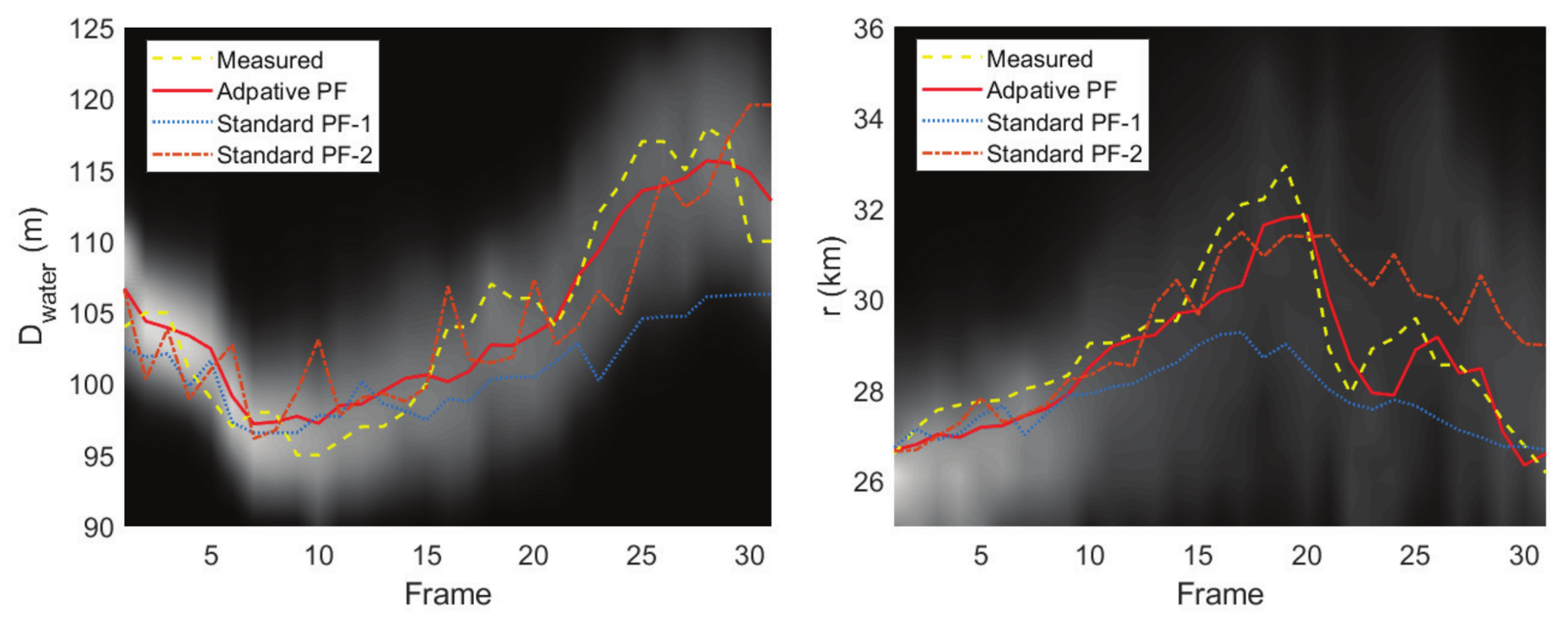
3.2. Interpretation of the Results

The results of the sequential geoacoustic parameters and the evolution of one-dimensional marginal PPDs of geoacoustic parameters and the source–receiver distance are provided in Figure 6, where solid lines denote the estimated values of each parameter. The 10,000 APF starts with initial covariance C 0 , which is set to diag [ ( x + x ) / 2 ] 2 to ensure that initial particles cover the entire parameter intervals. The PPDs are provided in terms of the normalized histograms from all particles. For comparison, the results of the independent genetic algorithm (GA) inversions of every WBS signal are also marked as isolated points in Figure 6. A detailed discussion of this comparison is given in the next section.
The geoacoustic parameters in the top layer show significant changes because both low- and high-frequency signals can interact with this layer. Furthermore, the top layer is distinctive because this layer has two sound speed parameters, in the top and bottom. In previous works [1,3,4,23] (both inversion results and core data), this layer was found to be thinner than other layers and had a relatively high gradient of sound speed, which is also found in our results. The gravity core data that penetrate down to a maximum depth of 1 m were taken along the propagation path, showing the surface sediment speed were in the range of 1570–1675 m/s [1]. The sequential inversion results of the nearest sites (frames 5–6) describe a similar sound speed range of 1580–1630 m/s for the surface sediment layer.
The evolution of parameters in the second layer shows their spatially-distributed properties: the equivalent thickness increases to 38 m and then decreases to about 20 m while sound speed shows the opposite trend. As a reference, Yang et al. [4] obtained the inversion results of this site using the multi-step matched-field method. The matched-field inversion results of an environmental model with one sediment layer indicated that the sound speed of the northwestern (NW) sediment is significantly smaller than on the southeastern (SE) and southwestern (SW) sides. The evolution of c sed 1 and c sed 2 in Figure 6 show a similar change from SW to NW (frames 1 to 12). Potty et al. [1] used the sediment tomography technique with a hybrid method to invert the sound speed profiles (Figure 13 in [1] and the location is near frame 5 in our work). Their results showed that the sound speed in the top layer increased from 1590 to 1665 m/s and that of the sediment above the basement was 1640 m/s. The basement sound speed was approximately 1685 m/s. These values compare well with our results in Figure 6. Similar results of sediment speed estimation were also reported by Reference [23] and the signal was collected near the center of the circle (position M in Figure 6a). Due to the limitation of the frequency band, it is difficult for signals to interact with the deeper layer, so the credibility of the inversion results in the basement is relatively lower than that of the layers above. Table 2 summarizes the comparison with the relevant geoacoustic parameters discussed above.
The first three EOF coefficients were used to consider the time-varying sound speed profile and their tracking results are also provided. An interesting finding is that the most fluctuating parameter was 2-EOF. The possible reason for this finding is that the variation in the sound speed profile in the selected time period (10 h) was relatively minimal, resulting in fewer fluctuations in the 1-EOF coefficient, which plays a major role compared with the remaining EOF coefficients.
To verify the reliability of the inversion method and results, it is feasible to apply the estimated model parameters to another source [2]. In this work, we chose a set of geoacoustic parameters estimated on a circular track and bring them to a location where another WBS signal was dropped to compare the dispersion curves. The observed dispersion curves were extracted by the warping transform introduced in Section 3.1. Figure 7a,b shows the comparison of dispersion curves. The environment parameters (excluding r, as r was measured by GPS) in the chosen location (thick green dashed line in Figure 7a) were used to compute the predicted dispersion curves in the location marked with a blue pentagram and the comparison result is provided as a time–frequency spectrogram in Figure 7b. As can be seen in this figure, the observed dispersion curves and predicted curves are in good agreement at most frequency points, indicating that the inversion results are reliable in this area. To validate the sequential estimation method, the estimated geoacoustic parameters at each frame were used to compute the predicted transmission loss (TL) at different frequencies then they are used to compare with experiment TL. Figure 7c shows the TL at six frequencies with a receiver depth of 70.6 m. We can find that the predicted and experimental TL are consistent for most frames and the root mean square error at different frequencies are all essentially less than 3 dB.

4. Discussion

A comparison is provided for the proposed method and the independent inversion method. For example, GA inversion is a widely-used independent geoacoustic inversion method. Figure 6 also depicts the independent GA inversion results for the same data set and its results are marked as discrete points. In this work, GA inversion needed at least 300 iterations with a population size of 200 to converge, so it requires 60,000 forward model runs for a single measurement. GA is computed independently each time; the previous result and probability distribution cannot be used for the next search, so it needs more time to run the forward model, resulting in unnecessary calculation waste. GA tends to fall into local optima. For this reason, we found that the GA inversion results show stronger fluctuations. To avoid this problem, GA needs a larger population size, resulting in larger computational consumption. As a comparison, the APF method shows advantages in terms of a small calculation amount and robust behavior with small variation. Because the time consumption in the inverse calculation is due to the calls to forward model, the lower the total number of calls, the shorter the time consumption. In our work, the APF requires only one-sixth of the computation time of GA.
In addition, compared with other sequential inversion methods, APF has its own advantages. Due to complexity and nonlinearities, sequential geoacoustic inversion applications require filters to handle such problems. A tough problem of PF geoacoustic inversion method is the “blind ” prediction because it cannot use the information in the latest observation [13]. As for APF used in this work, it achieves tracking inversion of geoacoustic parameters in a changing environment with a small increase in computational consumption using advance adaptive scaling and pre-shift. The comparison of performance can be obtained by tracking the parameters with measured values.
In this work, the water depth d w a t e r can be verified using database results, and source–receiver distance r can be calculated from the GPS. As mentioned above, the tracking results of water depth d w a t e r and source–receiver distance r show obvious changes from start to end. Figure 8 provides the detailed sequential estimation results of water depth d water and source–receiver distance r. For illustration purposes, the sequential estimation is implemented by the PF with different control parameters, and the results are also given in Figure 8. In the tracking of d water , the diagonal term in state noise Q k 1 / 2 is 3 m for standard PF-1 and 9 m for standard PF-2. Because the R/V sailed in a clockwise direction, the water depth changed from 105 to 90 m in the first 10 frames, then dropped to about 110 m, and finally returned to 105 m. The west part of the trajectory is a gentle slope, so the estimations of water depth are relatively accurate for APF and Standard PF-1. The situation is different in the east part because the slope steepens. The standard PF-1 loses track of d water from frame 15. However, standard PF-2 shows large oscillations in many frames, leading considerable error.
Likewise, the diagonal term in state noise Q k 1 / 2 is 500 m for standard PF-1 and 1000 m for standard PF-2 in the tracking of r. The track shows that r rapidly increases from 26 to 33 km and then back to 26 km, which is consistent with the intuitive sense of the results in Figure 2. Notably, because the track of the R/V is not a perfect circle on the northeast side of the VLA, there is a distinct notch in the varying distance value from frames 20 to 25. For r, the proposed method performs well throughout the tracking process, even in the notched part. The average error in the tracking of r is less than 5%.
The results show small state noise causes tracking failure and large state noise leads to oscillation or divergence. The standard PF depends on a fixed state noise matrix Q k , whose value is difficult to balance in these two situations. However, APF can adjust the covariance matrix C ^ k | k 1 with the latest observation. As for these parameters, C ^ k | k 1 remains unchanged when the variation range is relatively small and expands immediately to sampling particles in a wider range when it varies quickly, so the estimations are always near the high-likelihood area.

5. Summary and Conclusions

In summary, in this study, we investigated the application of adaptive PF for sequentially estimating geoacoustic and source parameters with modal dispersion curves. Compared with independent inversion, the proposed method produces a more stable and smooth inversion result and significantly saves computation time. Additionally, the correlations of different parameters are used in the sequential inversion. The proposed method uses adaptive shift for particles and the covariance matrix of state noise is updated online so it can adjust itself in a rapidly varying environment. This approach was demonstrated on the experimental data collected from ASIAEX 2001 and the results of water depth as well as source–receiver distance shows that the proposed method has the smallest average error compared with standard PF. For this experiment, previous studies did not mention the deviation in each WBS emission position in the circular trajectory, whereas the proposed method achieves tracking of source–receiver distance, even in rapidly changing environments.

Author Contributions

Conceptualization, H.L.; methodology, H.L.; software, H.L.; writing: original draft preparation, H.L.; writing: review and editing, H.L.and Q.Y.; supervision, K.Y. All authors have read and agreed to the published version of the manuscript.

Funding

This work was supported by the Fundamental Research Funds for the Central Universities of China (Grant No. 3102019HHZY03011), National Natural Science Foundation of China (Grant Nos. 42076198 and 61901383), the China Postdoctoral Science Foundation (Grant Nos. 2019M663822 and 2020M670246) and the Open Fund Project of Key Laboratory of Marine Environmental Information Technology, Ministry of Natural Resources of the People’s Republic of China.

Conflicts of Interest

All the authors have no conflicts of interest to declare.

References

  1. Potty, G.R.; Miller, J.H.; Dahl, P.H.; Lazauski, C.J. Geoacoustic inversion results from the ASIAEX East China Sea experiment. IEEE J. Ocean. Eng. 2004, 29, 1000–1010. [Google Scholar] [CrossRef]
  2. Guo, X.L.; Yang, K.D.; Ma, Y.L.; Yang, Q.L. Geoacoustic Inversion Based on Modal Dispersion Curve for Range-Dependent Environment. Chin. Phys. Lett. 2015, 32, 124302. [Google Scholar] [CrossRef]
  3. Dahl, P.H.; Zhang, R.; Miller, J.H.; Bartek, L.R.; Peng, Z.; Ramp, S.R.; Zhou, J.-X.; Chiu, C.-S.; Lynch, J.F.; Simmen, J.A.; et al. Overview of results from the Asian Seas International Acoustics Experiment in the East China Sea. IEEE J. Ocean. Eng. 2004, 29, 920–928. [Google Scholar] [CrossRef] [Green Version]
  4. Yang, K.; Ma, Y.; Sun, C.; Miller, J.H.; Potty, G.R. Multistep matched-field inversion for broad-band data from ASIAEX2001. IEEE J. Ocean. Eng. 2004, 29, 964–972. [Google Scholar] [CrossRef]
  5. Xu, L.; Yang, K.; Yang, Q. Experimental Study of Geoacoustic Inversion with Reliable Acoustic Path in the Philippine Sea. J. Theor. Comput. Acoust. 2019, 27, 1850061. [Google Scholar] [CrossRef]
  6. Bonnel, J.; Dosso, S.E.; Ross Chapman, N. Bayesian geoacoustic inversion of single hydrophone light bulb data using warping dispersion analysis. J. Acoust. Soc. Am. 2013, 134, 120–130. [Google Scholar] [CrossRef] [PubMed]
  7. Guo, X.; Yang, K.; Duan, R.; Ma, Y. Sequential Inversion for Geoacoustic Parameters in the South China Sea Using Modal Dispersion Curves. Acoust. Aust. 2017, 45, 1–11. [Google Scholar] [CrossRef]
  8. Bonnel, J.; Thode, A.; Wright, D.; Chapman, R. Nonlinear time-warping made simple: A step-by-step tutorial on underwater acoustic modal separation with a single hydrophone. J. Acoust. Soc. Am. 2020, 147, 1897–1926. [Google Scholar] [CrossRef] [PubMed] [Green Version]
  9. Liu, H.; Yang, K.; Ma, Y.; Yang, Q.; Huang, C. Synchrosqueezing transform for geoacoustic inversion with air-gun source in the East China Sea. Appl. Acoust. 2020, 169, 107460. [Google Scholar] [CrossRef]
  10. Yardim, C.; Michalopoulou, Z.; Gerstoft, P. An Overview of Sequential Bayesian Filtering in Ocean Acoustics. IEEE J. Ocean. Eng. 2011, 36, 71–89. [Google Scholar] [CrossRef]
  11. Doucet, A.; de Freitas, N.; Gordon, N. An Introduction to Sequential Monte Carlo Methods; Springer: New York, NY, USA, 2001. [Google Scholar] [CrossRef]
  12. Yardim, C.; Gerstoft, P.; Hodgkiss, W.S. Geoacoustic and source tracking using particle filtering: Experimental results. J. Acoust. Soc. Am. 2010, 128, 75–87. [Google Scholar] [CrossRef] [Green Version]
  13. Yardim, C.; Gerstoft, P.; Hodgkiss, W.S. Sequential geoacoustic inversion at the continental shelfbreak. J. Acoust. Soc. Am. 2012, 131, 1722–1732. [Google Scholar] [CrossRef]
  14. Cappe, O.; Godsill, S.J.; Moulines, E. An Overview of Existing Methods and Recent Advances in Sequential Monte Carlo. Proc. IEEE 2007, 95, 899–924. [Google Scholar] [CrossRef]
  15. Musso, C.; Oudjane, N.; Le Gland, F. Improving Regularised Particle Filters. In Sequential Monte Carlo Methods in Practice; Doucet, A., de Freitas, N., Gordon, N., Eds.; Springer: New York, NY, USA, 2001; pp. 247–271. [Google Scholar] [CrossRef]
  16. Gilks, W.R.; Berzuini, C. Following a moving target—Monte Carlo inference for dynamic Bayesian models. J. R. Stat. Soc. Ser. B Stat. Methodol. 2001, 63, 127–146. [Google Scholar] [CrossRef]
  17. Li, J.; Zhou, H. Tracking of time-evolving sound speed profiles in shallow water using an ensemble Kalman-particle filter. J. Acoust. Soc. Am. 2013, 133, 1377–1386. [Google Scholar] [CrossRef]
  18. Bo, L.; Xiong, J.; Ma, S. Sequential inversion of self-noise using adaptive particle filter in shallow water. J. Acoust. Soc. Am. 2018, 143, 2487–2500. [Google Scholar] [CrossRef]
  19. Dosso, S.E.; Dettmer, J. Bayesian matched-field geoacoustic inversion. Inverse Probl. 2011, 27, 55009. [Google Scholar] [CrossRef] [Green Version]
  20. Porter, M.B.; Reiss, E.L. A numerical method for bottom interacting ocean acoustic normal modes. J. Acoust. Soc. Am. 1985, 77, 1760–1767. [Google Scholar] [CrossRef]
  21. Zhang, X.D.; Wu, L.X.; Niu, H.Q.; Zhang, R.H. Sequential Parameter Estimation Using Modal Dispersion Curves in Shallow Water. Chin. Phys. Lett. 2018, 35, 44301. [Google Scholar] [CrossRef]
  22. Hamilton, E.L.; Bachman, R.T. Sound velocity and related properties of marine sediments. J. Acoust. Soc. Am. 1982, 72, 1891–1904. [Google Scholar] [CrossRef]
  23. Miller, J.H.; Bartek, L.R.; Potty, G.R.; Tang, D.; Na, J.; Qi, Y. Sediments in the East China Sea. IEEE J. Ocean. Eng. 2004, 29, 940–951. [Google Scholar] [CrossRef]
Figure 1. The comparison of standard PF and adaptive PF in a single iteration.
Remotesensing 13 02387 g001
Figure 2. Location of the ASIAEX 2001 experiment site and the SSP used in this paper. The bathymetry is obtained from the ETOPO1. (a) M (red square) is the designed center of a circle and VLA (black triangle) is the actual location of deployed. The blue circle is the first WBS signal and the red clockwise curve is the real trajectory of sound sources recorded by GPS. (b) The SSP were measured by CTD throughout the experiment period (about 9 days) and the average SSP (thick line).
Remotesensing 13 02387 g002
Figure 3. EOFs of measured SSPs. (a) the first four EOFs. (b) Percent of total fit energy with limited sets of EOFs.
Remotesensing 13 02387 g003
Figure 4. The illustration of extracting modal dispersion curves with the first WBS signal. The time domain signals received by VLA are shown in (a). The left side is the channel number and the right side is the corresponding depth. The signal received at 78.6 m is shown in (b) and its short-time Fourier spectrogram is given in (d). The warped spectrogram is shown in (c), where warped modes are approximately horizontal. Extracted (black) and modeled (white) dispersion curves are superimposed on the time-frequency spectrogram in (d).
Remotesensing 13 02387 g004
Figure 5. The model selection study of seabed. (a) Results of the model selection study. From top to bottom are misfit, number of parameters and BIC values as functions of number of seabed layers. For display purposes, BIC values are shifted so the minimum is at unity and plotted on a log scale. (b) The model of three layers (two sediment layers with basement) is selected in sequential estimations.
Remotesensing 13 02387 g005
Figure 6. The evolution of marginal PPDs, estimation results (solid lines) and GA results (*) for sediment parameters, basement sound speed, source range, water depth, d t , and the first three EOF coefficients. The dashed lines denote the water depth from ETOPT1 and the real source-receiver distance from GPS, respectively.
Remotesensing 13 02387 g006
Figure 7. The verification of inversion. Two locations used in comparison of dispersion curve are marked in (a): the geoacoustic parameters of green dashed line is used to compute predicted dispersion curves at the location of blue pentagram. The time–frequency spectrogram is shown in (b) with observed (black) and predicted (white) dispersion curves. (c) Predicted TL (solid lines) in circular track compared with experiment data (dashed lines). Frequency is shown in each subplot.
Remotesensing 13 02387 g007
Figure 8. The tracking of d water and r. The dashed line denotes the measured range of source from GPS and solid line gives the estimations of adaptive PF. The dotted line is the result of standard PF-1 and the dash-dotted line is standard PF-2.
Remotesensing 13 02387 g008
Table 1. The search bounds, reference information for the APF, and the initial setting from the MAP modal of the first signal.
BoundsInitial Value BoundsInitial Value
c sed 1 upper (m/s)[1530 1690]1580.7 d water (m)[90 125]106.1
Δ c sed 1 lower (m/s)[20 80]40.1 d sed 1 (m)[1 10]4.1
c sed 2 (m/s)[1600 1690]1647.2 d sed 2 (m)[1 40]29.7
c bot (m/s)[1640 1790]1687.01-EOF[−50 50]−9.2
r (km)[25 36]27.102-EOF[−20 20]−2.2
d t (s)[−1 1]0.0133-EOF[−15 15]−2.0
Table 2. Comparison of parameters estimated here with those of other studies. The gravity core data were measured from the surface of the seabed and are presented as a confidence interval. The results in the last column were obtained from the site closest to the measurement point in our study.
StudyGeoacoustic ParametersResultResult in This Study
Gravity core data(Ref. [23])Surface sound speed1570–1675 m/s1580–1630 m/s
Potter et al. (Ref. [1])[ c sed 1 upper , c sed 1 lower ][1590, 1665] m/s[1580, 1630] m/s
Potter et al. (Ref. [1]) c sed 2 1640 m/s1618 m/s
Potter et al. (Ref. [1]) c bot 1685 m/s1670 m/s
Yang et al. (Ref. [4]) c sed 1 upper 1594.4 m/s1609 m/s
Publisher’s Note: MDPI stays neutral with regard to jurisdictional claims in published maps and institutional affiliations.

