
Investigating the Temporal and Spatial Dynamics of Human Development Index: A Comparative Study on Countries and Regions in the Eastern Hemisphere from the Perspective of Evolution


Abstract
:
1. Introduction
2. Data and Methods
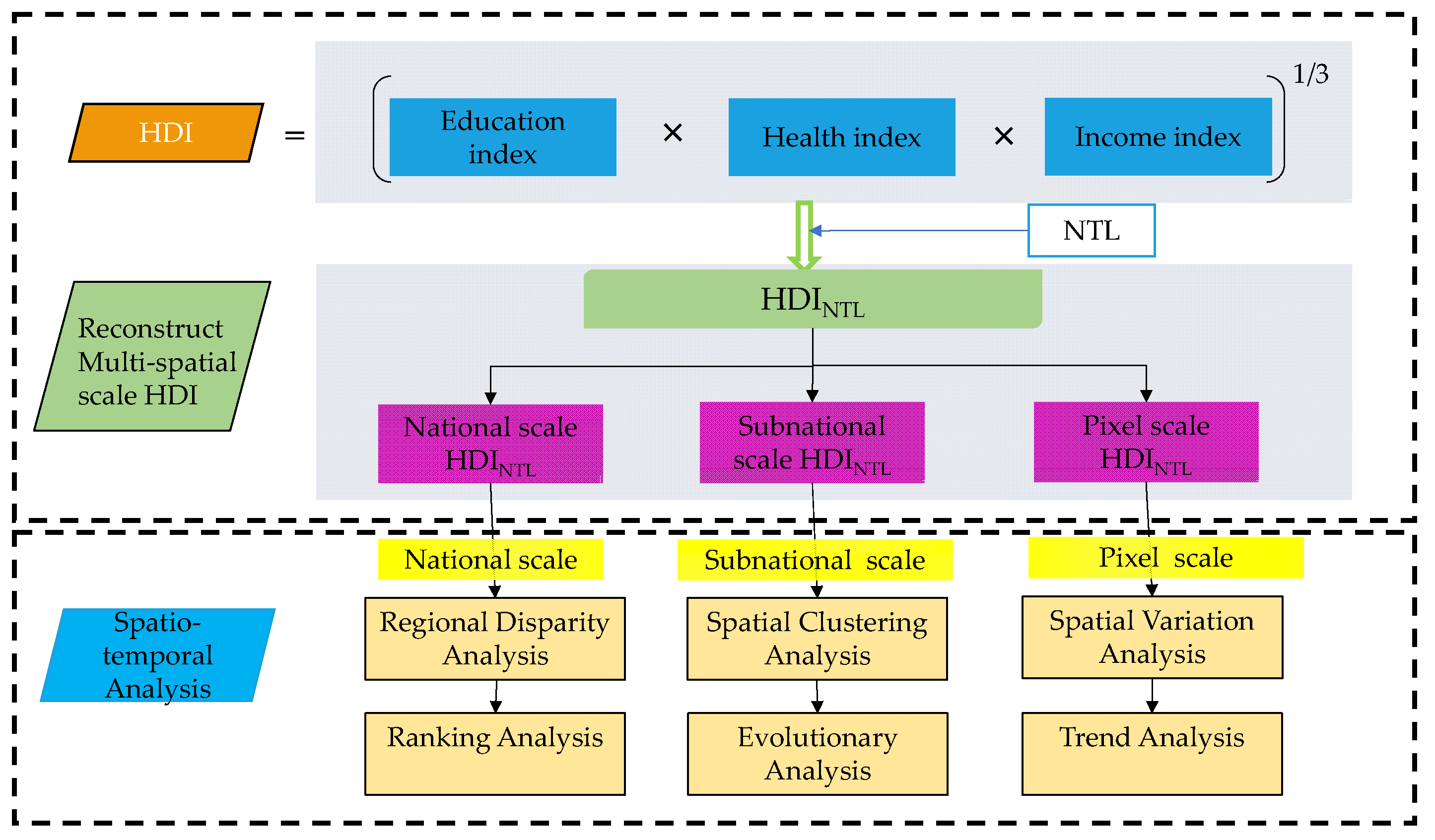
2.1. Study Area
2.2. Data and Preprocessing
2.3. Methods
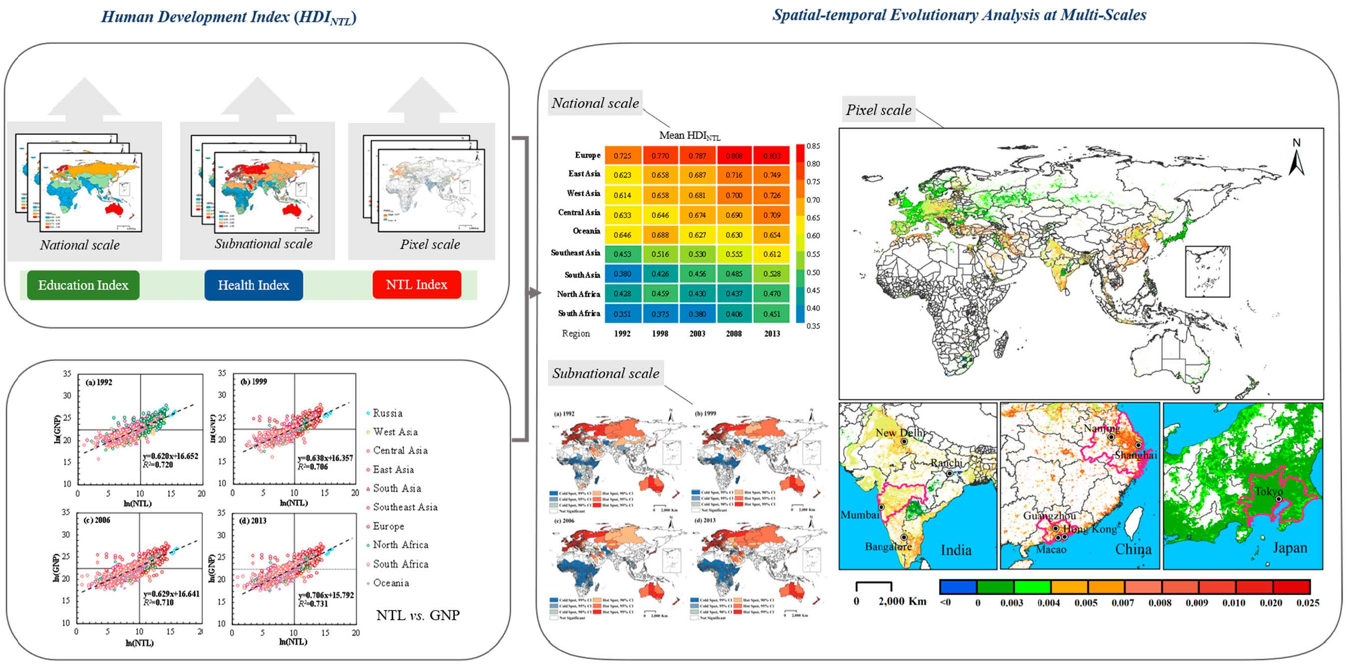
2.3.1. NTL-Based Human Development Indexes (HDINTL)
2.3.2. Spatial Autocorrelation Analysis
2.3.3. Trend Analysis (Slope)
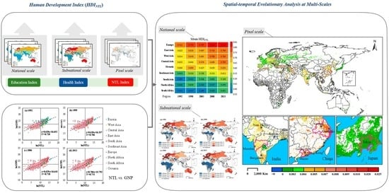
3. Results and Discussion
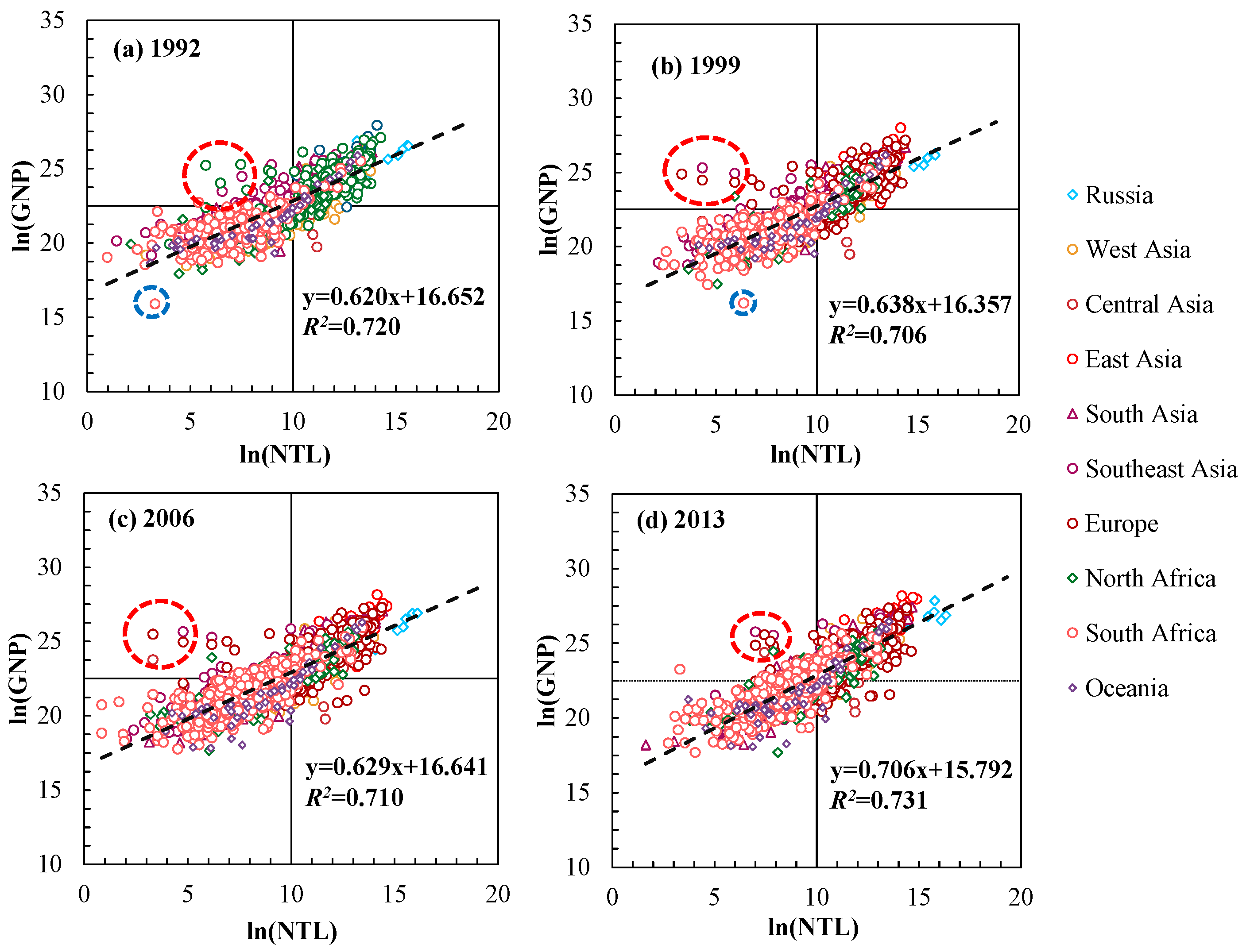
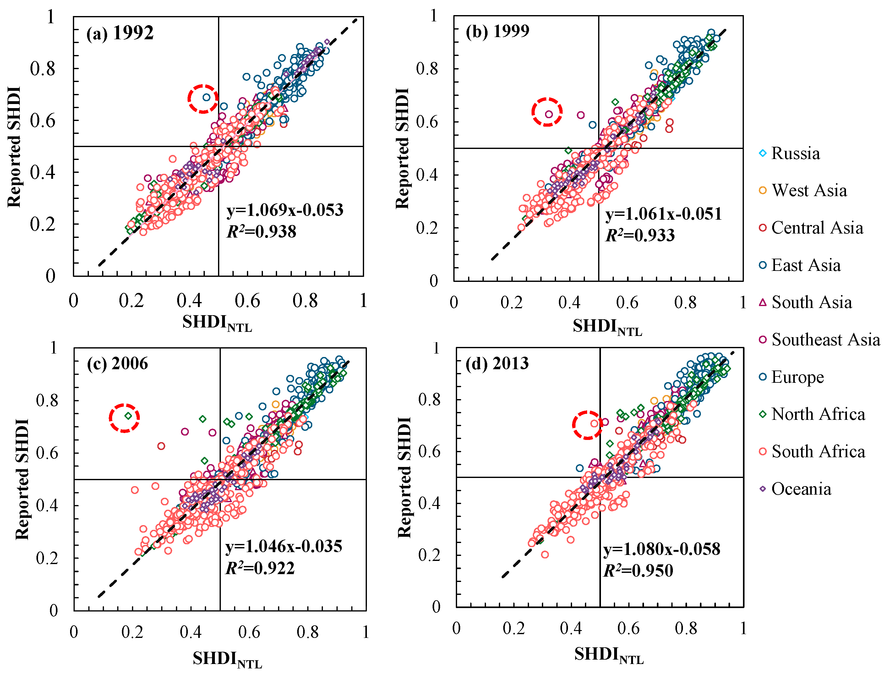
3.1. Performance Analysis of HDINTL
3.2. Spatiotemporal Analysis of HDINTL at the National Scale
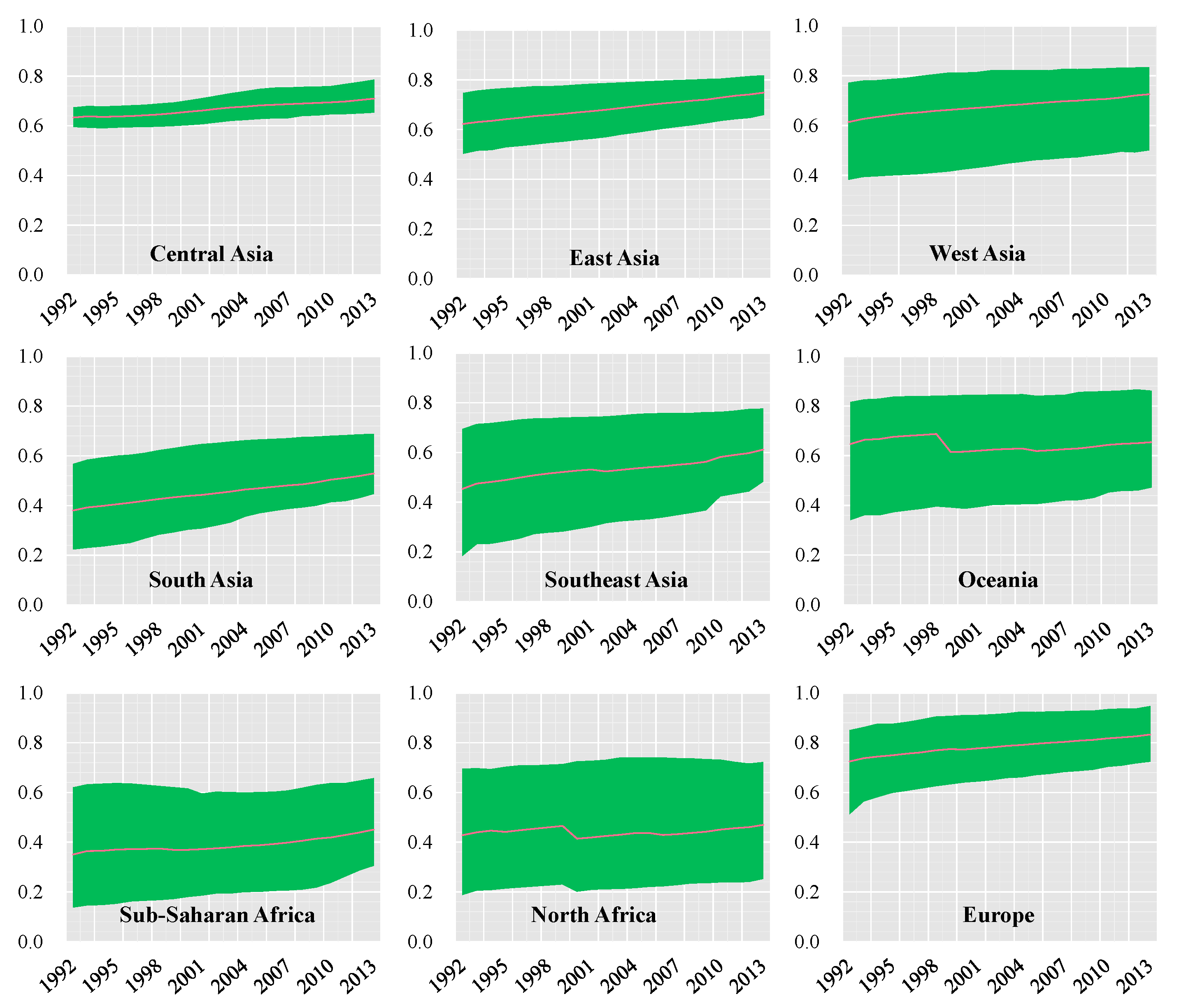
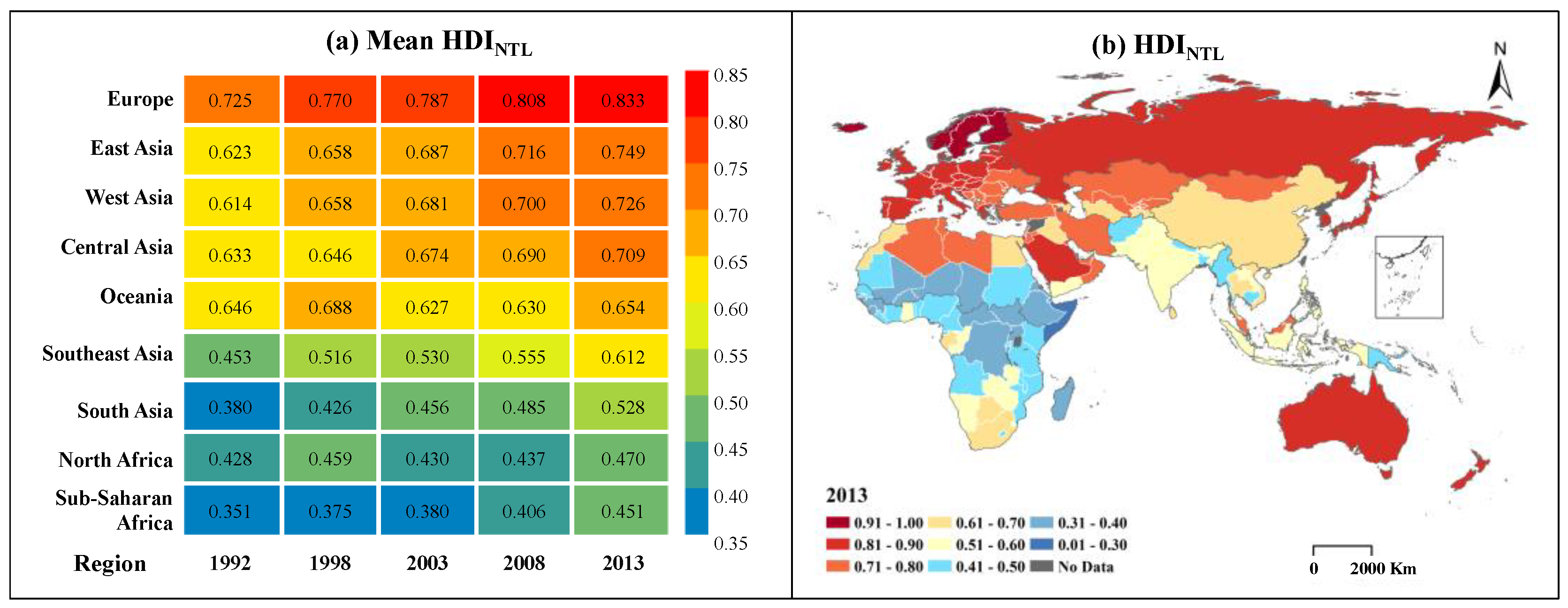
3.2.1. Regional Disparity Analysis
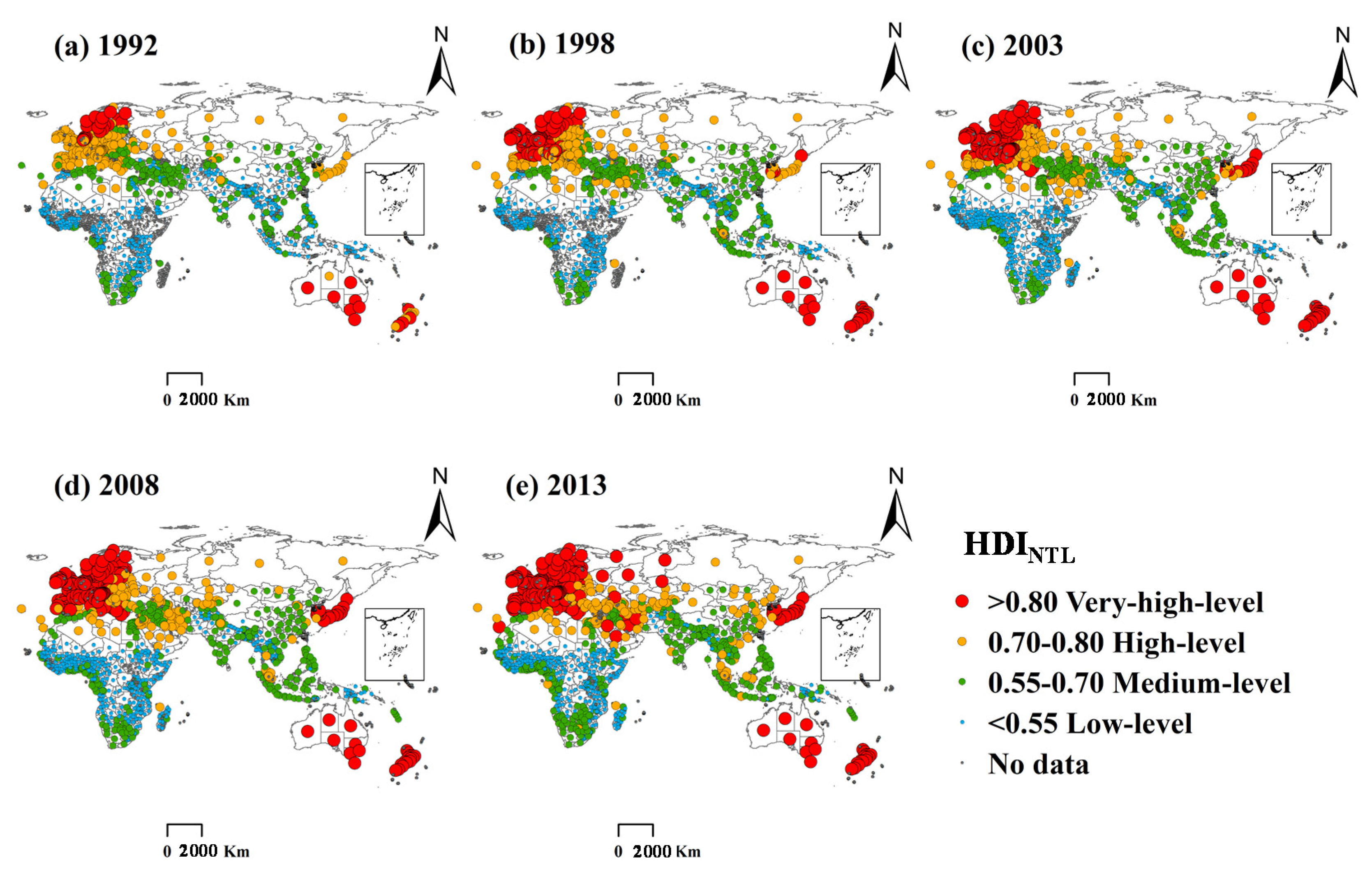
3.2.2. Ranking Analysis
3.3. Spatiotemporal Analysis of HDINTL at the Subnational Scale
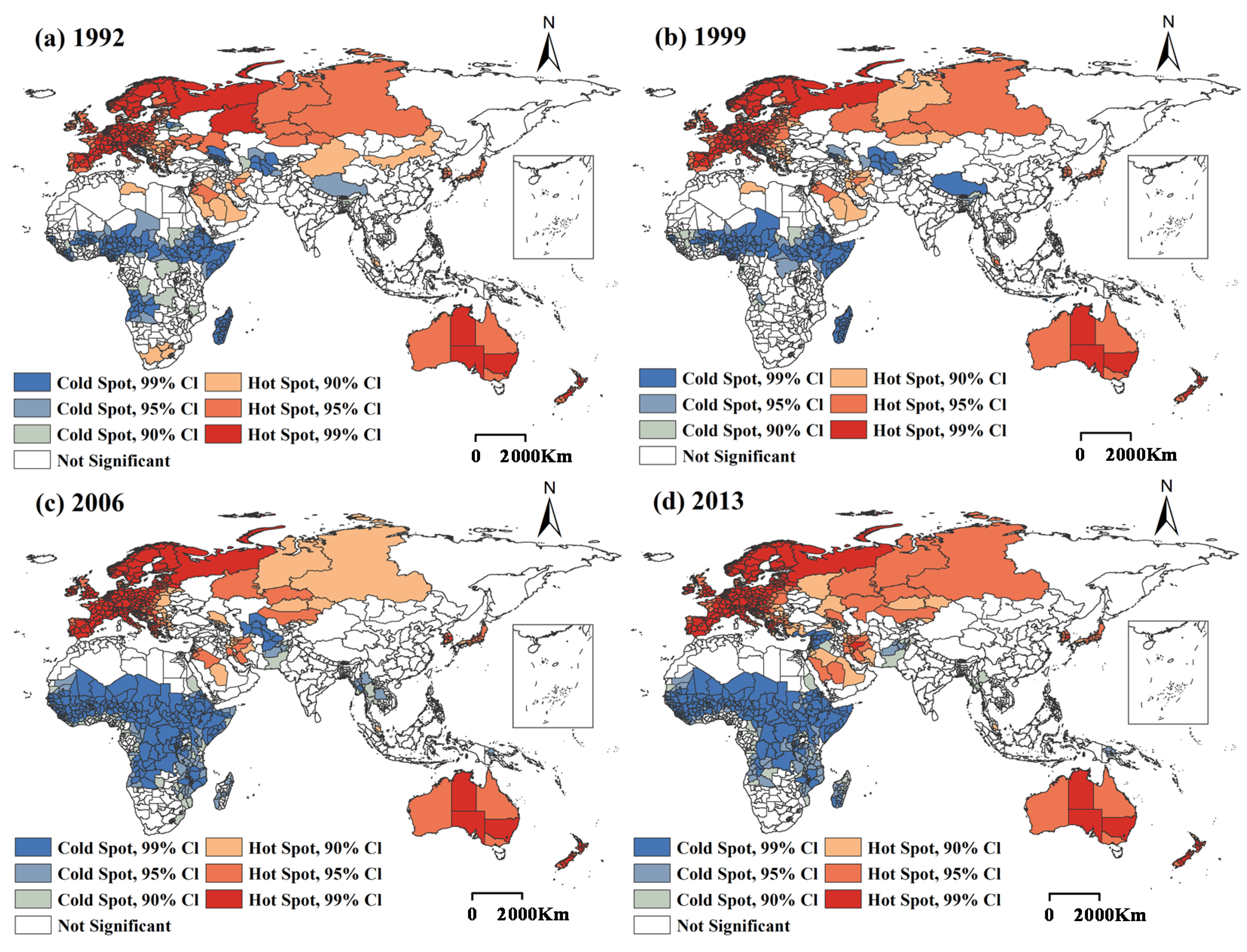
3.3.1. Spatial Clustering Analysis
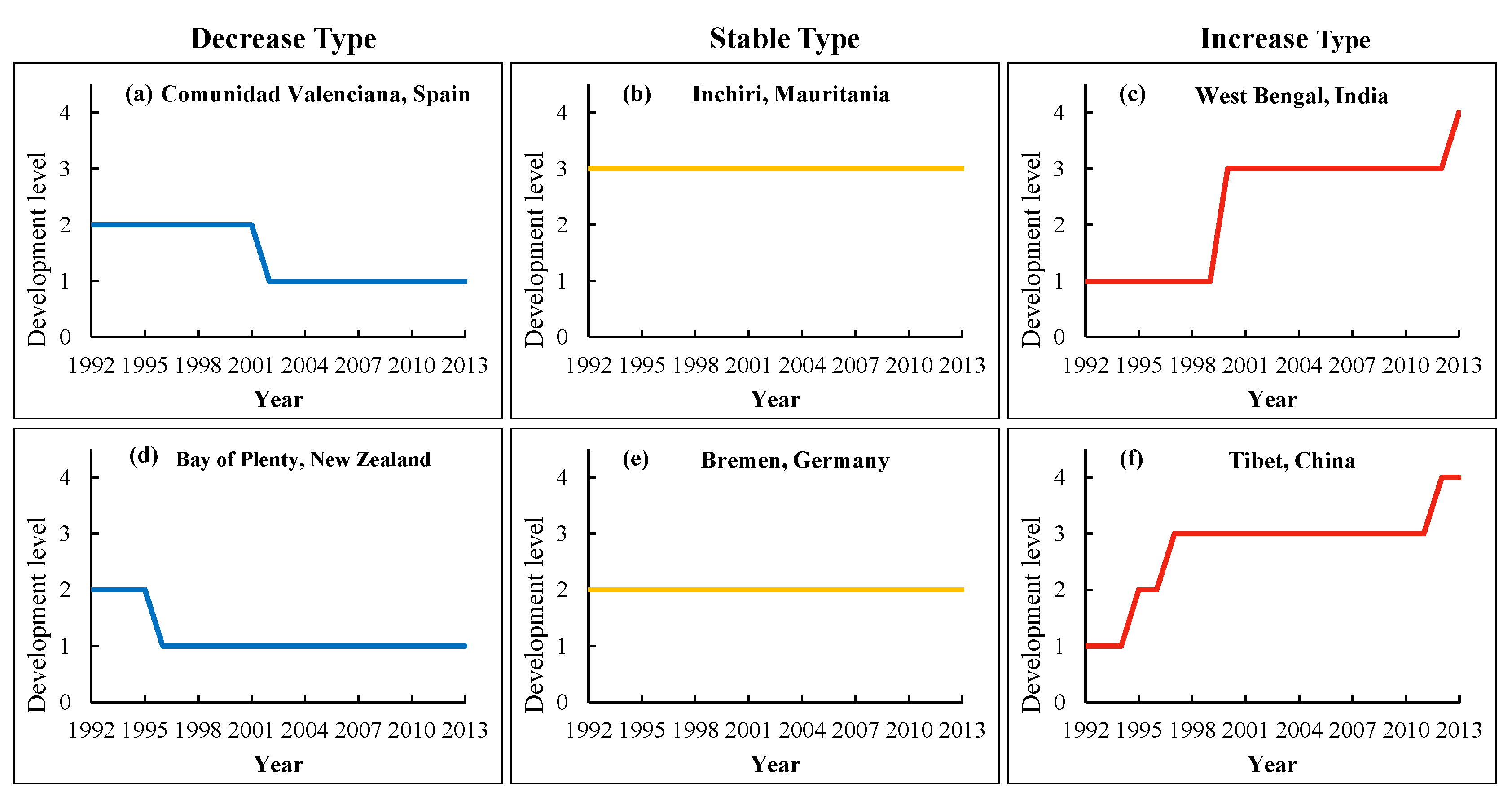
3.3.2. Evolutionary Analysis
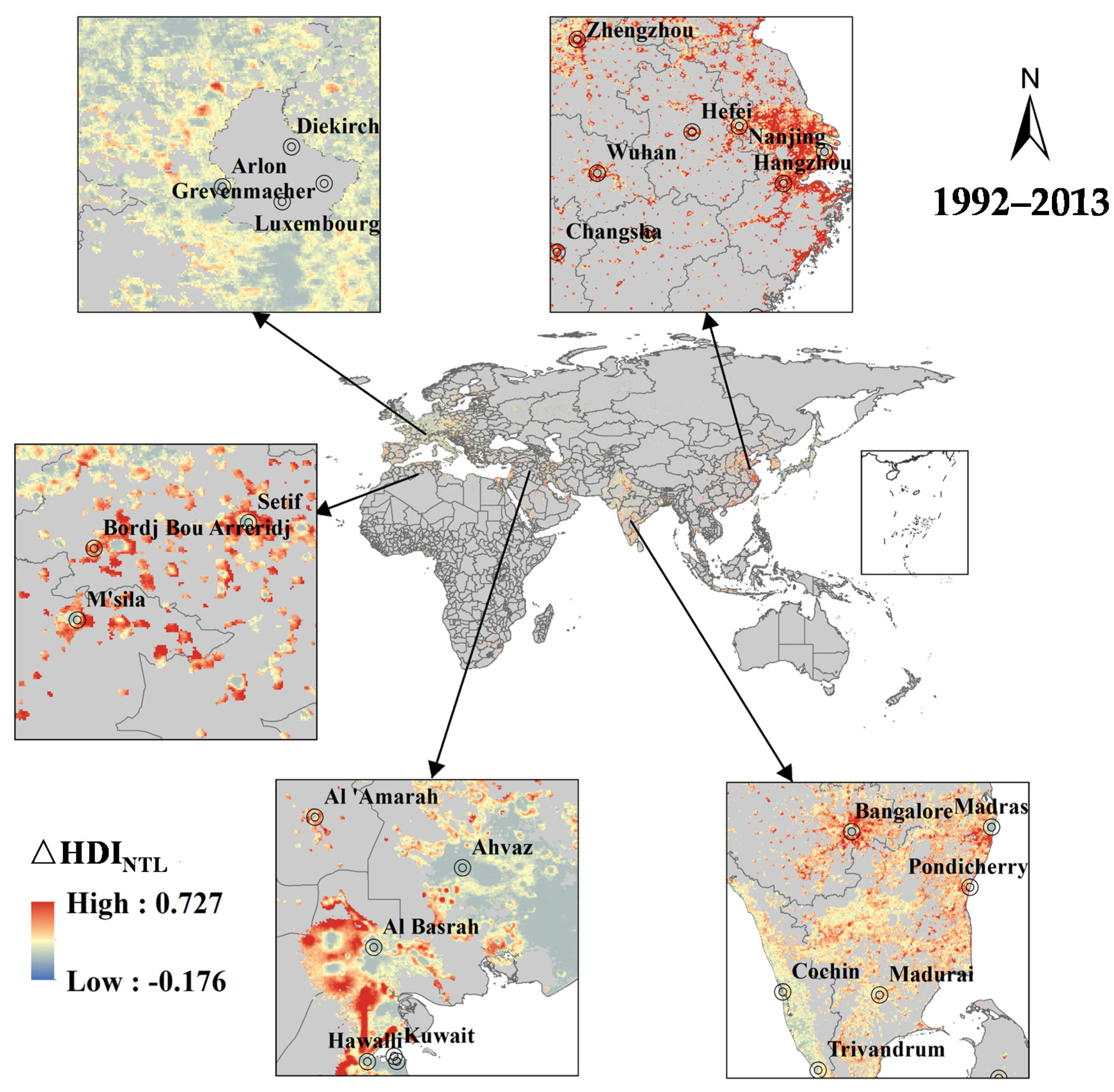
3.4. Spatiotemporal Analysis of HDINTL at the Pixel Scale
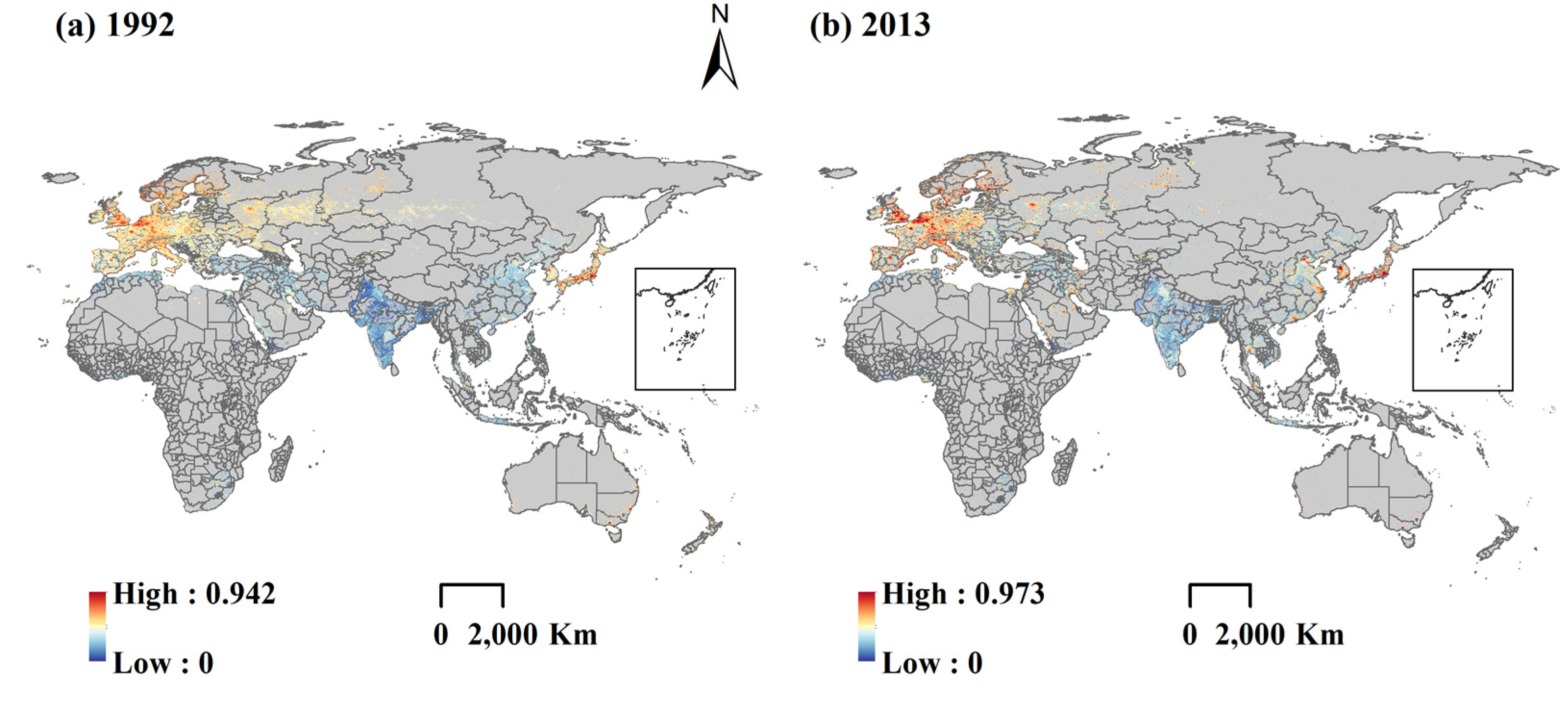
3.4.1. Spatial Variation Analysis
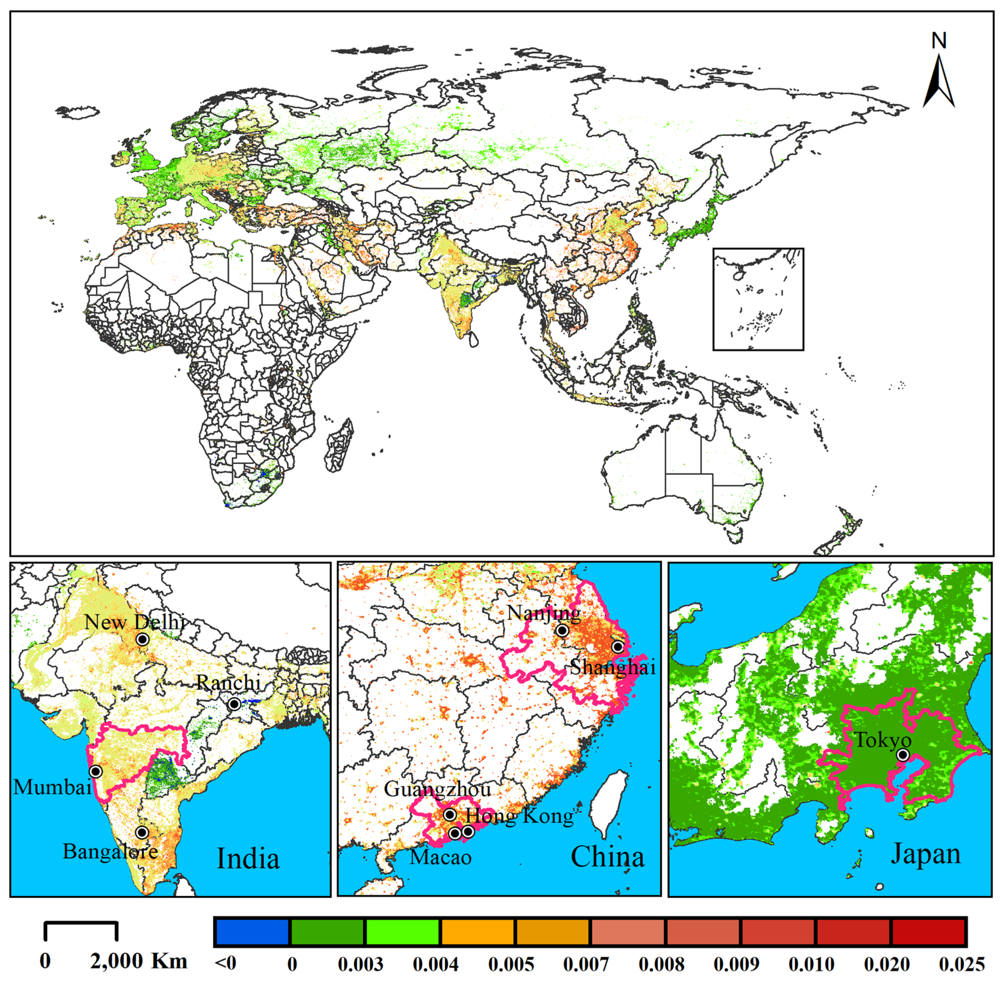
3.4.2. Trend Analysis
4. Conclusions and Policy Implications
4.1. Conclusions
4.2. Policy Implications
Supplementary Materials
Author Contributions
Funding
Acknowledgments
Conflicts of Interest
Abbreviation
| Abbreviations | Full Names |
| DMSP/OLS | The Defense Meteorological Satellite Program’s Operational Linescan System |
| DN | Digital number values of nighttime lights |
| DNadjusted | Adjusted digital number values of nighttime lights |
| GNP | Gross national product |
| HDI | Human Development Index |
| HDINTL | New Human Development Index reconstructed using nighttime lights |
| NHDINTL | The national HDINTL |
| ΔPHDINTL | The HDINTL change value at each pixel during 1992–2013 |
| PHDINTL1992 | The HDINTL value at each pixel in 1992 |
| PHDINTL2013 | The HDINTL value at each pixel in 2013 |
| Ieducation | Education Index |
| IHealth | Health Index |
| INTL | NTL Index, the index calculated by nighttime lights data |
| NOAA/NGDC | National Oceanic and Atmospheric Administration’s National Geophysical Data Center |
| NLDI | Night light development index |
| NTL | Nighttime lights |
| ORNL | the Department of Energy’s Oak Ridge National Laboratory |
| PHDINTL | The HDINTL at pixel level |
| PHDIadjusted | The adjusted HDINTL at pixel level |
| ΔPHDINTL | The HDINTL change value at each pixel during 1992–2013 |
| PHDINTL1992 | The HDINTL value at each pixel in 1992 |
| PHDINTL2013 | The HDINTL value at each pixel in 2013 |
| SDGs | Sustainable development goals |
| SHDI | The data published by Subnational Human Development Database |
| SHDINTL | The HDINTL at subnational level |
| SHDIadjusted | The adjusted HDINTL at subnational level |
| S-NPP VIIRS | Suomi-National Polar-orbiting Partnership |
| UNDP | United Nations Development Programme |
References
- Jing, C.; Tao, H.; Jiang, T.; Wang, Y.; Zhai, J.; Cao, L.; Su, B. Population, urbanization and economic scenarios over the Belt and Road region under the Shared Socioeconomic Pathways. J. Geogr. Sci. 2020, 30, 68–84. [Google Scholar] [CrossRef]
- Malik, K. Human Development Report 2013. The Rise of the South: Human Progress in a Diverse World (15 March 2013). UNDP-HDRO Human Development Reports. 2013. Available online: https://ssrn.com/abstract=2294673 (accessed on 14 June 2021).
- Martínez-Guido, S.I.; González-Campos, J.B.; Ponce-Ortega, J.M. Strategic planning to improve the Human Development Index in disenfranchised communities through satisfying food, water and energy needs. Food Bioprod. Process. 2019, 117, 14–29. [Google Scholar] [CrossRef]
- Biggeri, M.; Mauro, V. Towards a more ‘sustainable’ human development index: Integrating the environment and freedom. Ecol. Indicat. 2018, 91, 220–231. [Google Scholar] [CrossRef]
- Ladi, T.; Mahmoudpour, A.; Sharifi, A. Assessing impacts of the water poverty index components on the human development index in Iran. Habitat Int. 2021, 113, 102375. [Google Scholar] [CrossRef]
- Donohue, C.; Biggs, E. Monitoring socio-environmental change for sustainable development: Developing a Multidimensional Livelihoods Index (MLI). Appl. Geogr. 2015, 62, 391–403. [Google Scholar] [CrossRef]
- Dervis, K.; Klugman, J. Measuring human progress: The contribution of the Human Development Index and related indices. Rev. D’écon. Polit. 2011, 121, 73–92. [Google Scholar] [CrossRef]
- Spangenberg, J.H. The Corporate Human Development Index CHDI: A tool for corporate social sustainability management and reporting. J. Clean. Prod. 2016, 134, 414–424. [Google Scholar] [CrossRef]
- Neumayer, E. The human development index and sustainability—A constructive proposal. Ecol. Econ. 2001, 39, 101–114. [Google Scholar] [CrossRef]
- Klugman, J.; Rodríguez, F.; Choi, H.J. The HDI 2010: New controversies, old critiques. J. Econ. Inequal. 2011, 9, 249–288. [Google Scholar] [CrossRef]
- Sanusi, Y.A. Application of human development index to measurement of deprivations among urban households in Minna, Nigeria. Habitat Int. 2008, 32, 384–398. [Google Scholar] [CrossRef]
- Tian, Q.; Brown, D.G.; Bao, S.; Qi, S. Assessing and mapping human well-being for sustainable development amid flood hazards: Poyang Lake Region of China. Appl. Geogr. 2015, 63, 66–76. [Google Scholar] [CrossRef]
- Wang, Z.; Danish; Zhang, B.; Wang, B. Renewable energy consumption, economic growth and human development index in Pakistan: Evidence form simultaneous equation model. J. Clean. Prod. 2018, 184, 1081–1090. [Google Scholar] [CrossRef]
- Kummu, M.; Taka, M.; Guillaume, J.H.A. Gridded global datasets for gross domestic product and human development index over 1990–2015. Sci. Data 2018, 5, 180004. [Google Scholar] [CrossRef] [PubMed]
- Ji, X.; Li, X.; He, Y.; Liu, X. A simple method to improve estimates of county-level economics in China using nighttime light data and GDP growth rate. ISPRS Int. J. Geo-Inf. 2019, 8, 419. [Google Scholar] [CrossRef]
- Yee, S.H.; Paulukonis, E.; Buck, K.D. Downscaling a human well-being index for environmental management and environmental justice applications in Puerto Rico. Appl. Geogr. 2020, 123, 102231. [Google Scholar] [CrossRef]
- Jing, X.; Yan, Y.Z.; Yan, L.; Zhao, H. A novel method for saturation effect calibration of DMSP/OLS stable light product based on GDP grid data in China mainland at city level. Geogr. Geo Inf. Sci. 2017, 33, 35–39. [Google Scholar]
- Tan, M.; Li, X.; Li, S.; Xin, L.; Wang, X.; Li, Q.; Li, W.; Li, Y.; Xiang, W. Modeling population density based on nighttime light images and land use data in China. Appl. Geogr. 2018, 90, 239–247. [Google Scholar] [CrossRef]
- Li, X.; Zhou, W. Dasymetric mapping of urban population in China based on radiance corrected DMSP-OLS nighttime light and land cover data. Sci. Total Environ. 2018, 643, 1248–1256. [Google Scholar] [CrossRef]
- Ye, T.; Zhao, N.; Yang, X.; Ouyang, Z.; Liu, X.; Chen, Q.; Hu, K.; Yue, W.; Qi, J.; Li, Z.; et al. Improved population mapping for China using remotely sensed and points-of-interest data within a random forests model. Sci. Total Environ. 2019, 658, 936–946. [Google Scholar] [CrossRef]
- Dai, Z.; Hu, Y.; Zhao, G. The suitability of different nighttime light data for GDP estimation at different spatial scales and regional levels. Sustainability 2017, 9, 305. [Google Scholar] [CrossRef]
- Zhao, N.; Cao, G.; Zhang, W.; Samson, E.L. Tweets or nighttime lights: Comparison for preeminence in estimating socioeconomic factors. ISPRS J. Photogramm. Remote Sens. 2018, 146, 1–10. [Google Scholar] [CrossRef]
- Liang, H.; Guo, Z.; Wu, J.; Chen, Z. GDP spatialization in Ningbo City based on NPP/VIIRS night-time light and auxiliary data using random forest regression. Adv. Space Res. 2020, 65, 481–493. [Google Scholar] [CrossRef]
- Mellander, C.; Lobo, J.; Stolarick, K.; Matheson, Z. Night-time light data: A good proxy measure for economic activity? PLoS ONE 2015, 10, e0139779. [Google Scholar] [CrossRef] [PubMed]
- Jasiński, T. Modeling electricity consumption using nighttime light images and artificial neural networks. Energy 2019, 179, 831–842. [Google Scholar] [CrossRef]
- Cao, X.; Wang, J.; Chen, J.; Shi, F. Spatialization of electricity consumption of China using saturation-corrected DMSP-OLS data. Int. J. Appl. Earth Obs. Geoinf. 2014, 28, 193–200. [Google Scholar] [CrossRef]
- Dai, E.; Wang, Y. Attribution analysis for water yield service based on the geographical detector method: A case study of the Hengduan Mountain region. J. Geogr. Sci. 2020, 30, 1005–1020. [Google Scholar] [CrossRef]
- Liang, H.; Tanikawa, H.; Matsuno, Y.; Dong, L. Modeling in-use steel stock in China’s buildings and civil engineering infrastructure using time-series of DMSP/OLS nighttime lights. Remote Sens. 2014, 6, 4780–4800. [Google Scholar] [CrossRef]
- Liang, H.; Dong, L.; Tanikawa, H.; Zhang, N.; Gao, Z.; Luo, X. Feasibility of a new-generation nighttime light data for estimating in-use steel stock of buildings and civil engineering infrastructures. Resour. Conserv. Recycl. 2017, 123, 11–23. [Google Scholar] [CrossRef]
- Beyer, R.C.; Franco-Bedoya, S.; Galdo, V. Examining the economic impact of COVID-19 in India through daily electricity consumption and nighttime light intensity. World Dev. 2021, 140, 105287. [Google Scholar] [CrossRef]
- Levin, N.; Duke, Y. High spatial resolution night-time light images for demographic and socio-economic studies. Remote Sens. Environ. 2012, 119, 1–10. [Google Scholar] [CrossRef]
- Zhang, G.; Guo, X.; Li, D.; Jiang, B. Evaluating the potential of LJ1-01 nighttime light data for modeling socio-economic parameters. Sensors 2019, 19, 1465. [Google Scholar] [CrossRef]
- Gao, B.; Huang, Q.; He, C.; Dou, Y. Similarities and differences of city-size distributions in three main urban agglomerations of China from 1992 to 2015: A comparative study based on nighttime light data. J. Geogr. Sci. 2017, 27, 533–545. [Google Scholar] [CrossRef]
- Elvidge, C.D.; Baugh, K.E.; Anderson, S.; Sutton, P.; Ghosh, T. The Night Light Development Index (NLDI): A spatially explicit measure of human development from satellite data. Soc. Geogr. 2012, 7, 23–35. [Google Scholar] [CrossRef]
- Wu, J.; Wang, Z.; Li, W.; Peng, J. Exploring factors affecting the relationship between light consumption and GDP based on DMSP/OLS nighttime satellite imagery. Remote Sens. Environ. 2013, 134, 111–119. [Google Scholar] [CrossRef]
- He, C.; Ma, Q.; Liu, Z.; Zhang, Q. Modeling the spatiotemporal dynamics of electric power consumption in Mainland China using saturation-corrected DMSP/OLS nighttime stable light data. Int. J. Digit. Earth 2013, 7, 993–1014. [Google Scholar] [CrossRef]
- Zhao, M.; Cheng, W.; Zhou, C.; Li, M.; Wang, N.; Liu, Q. GDP spatialization and economic differences in south china based on NPP-VIIRS nighttime light imagery. Remote Sens. 2017, 9, 673. [Google Scholar] [CrossRef]
- National Remote Sensing Center of China (GEOARC). Global Ecosystems and Environment Observation Analysis Research Cooperation: The Belt and Road Initiative Ecological and Environmental Conditions. 2017. Available online: http://www.chinageoss.cn/geoarc/2017/pdf/ydyl2017_en.pdf (accessed on 14 June 2021).
- Herrmann, S.M.; Mohr, K.I. A continental-scale classification of rainfall seasonality regimes in africa based on gridded precipitation and land surface temperature products. J. Appl. Meteorol. Clim. 2011, 50, 2504–2513. [Google Scholar] [CrossRef]
- Smits, J.; Permanyer, I. The subnational human development database. Sci. Data 2019, 6, 190038. [Google Scholar] [CrossRef]
- Goldewijk, K.K.; Beusen, A.; Janssen, P. Long-term dynamic modeling of global population and built-up area in a spatially explicit way: HYDE 3.1. Holocene 2010, 20, 565–573. [Google Scholar] [CrossRef]
- Elvidge, C.D.; Ziskin, D.; Baugh, K.E.; Tuttle, B.T.; Ghosh, T.; Pack, D.W.; Erwin, E.H.; Zhizhin, M. A fifteen year record of global natural gas flaring derived from satellite data. Energies 2009, 2, 595–622. [Google Scholar] [CrossRef]
- Boots, B.; Tiefelsdorf, M. Global and local spatial autocorrelation in bounded regular tessellations. J. Geogr. Syst. 2000, 2, 319–348. [Google Scholar] [CrossRef]
- Hong, L.; Liang, N.; Di, W. Economic and environmental gains of China’s fossil energy subsidies reform: A rebound effect case study with EIMO model. Energy Policy 2013, 54, 335–342. [Google Scholar] [CrossRef]
- Xu, H.; Demetriades, A.; Reimann, C.; Jiménez, J.J.; Filser, J.; Zhang, C. Identification of the co-existence of low total organic carbon contents and low pH values in agricultural soil in north-central Europe using hot spot analysis based on GEMAS project data. Sci. Total Environ. 2019, 678, 94–104. [Google Scholar] [CrossRef]
- Elvidge, C.D.; Baugh, K.E.; Dietz, J.B.; Bland, T.; Sutton, P.; Kroehl, H.W. Radiance calibration of DMSP-OLS low-light imaging data of human settlements. Remote Sens. Environ. 1999, 68, 77–88. [Google Scholar] [CrossRef]
- Letu, H.; Hara, M.; Tana, G.; Nishio, F. A saturated light correction method for DMSP/OLS nighttime satellite imagery. IEEE Trans. Geosci. Remote Sens. 2012, 50, 389–396. [Google Scholar] [CrossRef]
- Sahoo, S.; Gupta, P.K.; Srivastav, S.K. Comparative analysis between VIIRS-DNB and DMSP-OLS night-time light data to estimate electric power consumption in Uttar Pradesh, India. Int. J. Remote Sens. 2019, 41, 2565–2580. [Google Scholar] [CrossRef]
- Shi, K.F.; Yu, B.L.; Huang, Y.X.; Hu, Y.J.; Yin, B.; Chen, Z.Q.; Chen, L.J.; Wu, J.P. Evaluating the ability of npp-viirs nighttime light data to estimate the gross domestic product and the electric power consumption of China at multiple scales: A comparison with DMSP-OLS Data. Remote Sens. 2014, 6, 1705–1724. [Google Scholar] [CrossRef]


| Region | Countries |
|---|---|
| Russia | Russian Federation |
| West Asia | Armenia, Azerbaijan, Cyprus, Georgia, Iran, Iraq, Israel, Jordan, Kuwait, Lebanon, Oman, Palestine, Qatar, Saudi Arabia, Syria, Turkey, United Arab Emirates, Yemen |
| Central Asia | Kazakhstan, Kyrgyzstan, Tajikistan, Turkmenistan, Uzbekistan |
| East Asia | China, Japan, South Korea, Mongolia |
| South Asia | Afghanistan, Bangladesh, Bhutan, India, Nepal, Pakistan, Sri Lanka |
| Europe | Albania, Andorra, Austria, Belarus, Belgium, Bosnia and Herzegovina, Bulgaria, Croatia, Czech Republic, Denmark, Estonia, Finland, France, Germany, Greece, Hungary, Iceland, Ireland, Italy, Latvia, Liechtenstein, Lithuania, Luxembourg, Moldova, Monte Negro, Netherlands, North Macedonia, Norway, Poland, Portugal, Romania, Serbia, Slovakia, Slovenia, Spain, Sweden, Switzerland, Ukraine, United Kingdom |
| Oceania | Australia, New Zealand, Papua New Guinea, Solomon Islands, Vanuatu |
| Southeast Asia | Brunei Darussalam, Cambodia, Indonesia, Lao, Malaysia, Myanmar, Philippines, Singapore, Thailand, Timor-Leste, Vietnam |
| North Africa | Algeria, Burkina Faso, Chad, Djibouti, Egypt, Eritrea, Ethiopia, Libya, Mali, Mauritania, Morocco, Niger, Somalia, Sudan, Tunisia |
| Sub-Saharan Africa | Angola, Benin, Botswana, Burundi, Cameroon, Cape Verde, Central African Republic CAR, Comoros, Congo Brazzaville, Congo Democratic Republic, Cote d’Ivoire, Equatorial Guinea, eSwatini, Gabon, Gambia, Ghana, Guinea, Guinea Bissau, Kenya, Lesotho, Liberia, Madagascar, Malawi, Mauritius, Mozambique, Namibia, Nigeria, Rwanda, Sao Tome and Principe, Senegal, Sierra Leone, South Africa, South Sudan, Tanzania, Togo, Uganda, Zambia, Zimbabwe |
| Category | Remarks | Source |
|---|---|---|
| Socioeconomic statistics data | Life expectancy at birth Mean years of schooling Expected years of schooling Gross national product (GNP) Population Reported HDI | The national level data is provided by the UNDP (http://hdr.undp.org/en/data/, accessed on 14 June 2021) at National, 1992–2013; The subnational level data is downloaded from the Subnational Human Development Database [40], 1992–2013. |
| Gridded population data | 5 arc-min (10 km at equator) 30 arc-sec (1 km at equator) | HYDE 3.1 Population Dataset [41], 1992–1999; Department of Energy’s Oak Ridge National Laboratory (ORNL) (https://landscan.ornl.gov/, accessed on 14 June 2021), 2000–2013. |
| Nighttime lights data | The DMSP-OLS NTL product (1 × 1 km) | NOAA/NGDC (http://ngdc.noaa.gov/eog/, accessed on 14 June 2021), 1992–2013. |
| Representative Countries | Region | 1992 | 1998 | 2003 | 2008 | 2013 | |||||
|---|---|---|---|---|---|---|---|---|---|---|---|
| NHDINTL | Rank | NHDINTL | Rank | NHDINTL | Rank | NHDINTL | Rank | NHDINTL | Rank | ||
| Finland | Europe | 0.819 | 3 | 0.870 | 3 | 0.897 | 3 | 0.924 | 2 | 0.947 | 1 |
| Iceland | Europe | 0.816 | 4 | 0.850 | 3 | 0.893 | 4 | 0.906 | 3 | 0.946 | 2 |
| Norway | Europe | 0.850 | 1 | 0.894 | 2 | 0.916 | 2 | 0.928 | 1 | 0.945 | 3 |
| Sweden | Europe | 0.833 | 2 | 0.905 | 1 | 0.918 | 1 | 0.904 | 4 | 0.935 | 4 |
| Denmark | Europe | 0.772 | 9 | 0.814 | 9 | 0.855 | 5 | 0.864 | 6 | 0.884 | 5 |
| Belgium | Europe | 0.798 | 6 | 0.836 | 5 | 0.847 | 7 | 0.858 | 7 | 0.866 | 8 |
| Representative Countries | Region | 1992 | 1998 | 2003 | 2008 | 2013 | |||||
|---|---|---|---|---|---|---|---|---|---|---|---|
| NHDINTL | Rank | NHDINTL | Rank | NHDINTL | Rank | NHDINTL | Rank | NHDINTL | Rank | ||
| Central African Republic CAR | Sub-Saharan Africa | 0.272 | 95 | 0.270 | 100 | 0.274 | 101 | 0.286 | 103 | 0.306 | 106 |
| Burundi | Sub-Saharan Africa | 0.180 | 103 | 0.215 | 105 | 0.231 | 105 | 0.269 | 104 | 0.313 | 105 |
| Sierra Leone | Sub-Saharan Africa | 0.138 | 105 | 0.168 | 106 | 0.194 | 106 | 0.210 | 106 | 0.315 | 104 |
| Niger | North Africa | 0.194 | 100 | 0.226 | 104 | 0.240 | 104 | 0.264 | 105 | 0.324 | 103 |
| Mali | North Africa | 0.188 | 101 | 0.248 | 101 | 0.295 | 100 | 0.333 | 100 | 0.359 | 102 |
| Guinea | Sub-Saharan Africa | 0.178 | 104 | 0.248 | 101 | 0.259 | 103 | 0.303 | 102 | 0.362 | 101 |
| Rwanda | Sub-Saharan Africa | 0.138 | 105 | 0.238 | 103 | 0.274 | 101 | 0.315 | 101 | 0.401 | 98 |
| Year | Moran’s I Values | z-Score | p-Value | Pattern | Year | Moran’s I Values | z-Score | p-Value | Pattern |
|---|---|---|---|---|---|---|---|---|---|
| 1992 | 0.772 | 45.484 | 0.000 *** | C | 2003 | 0.639 | 37.625 | 0.000 *** | C |
| 1993 | 0.771 | 45.424 | 0.000 *** | C | 2004 | 0.629 | 37.079 | 0.000 *** | C |
| 1994 | 0.772 | 45.454 | 0.000 *** | C | 2005 | 0.584 | 34.413 | 0.000 *** | C |
| 1995 | 0.772 | 45.464 | 0.000 *** | C | 2006 | 0.563 | 33.159 | 0.000 *** | C |
| 1996 | 0.771 | 45.422 | 0.000 *** | C | 2007 | 0.562 | 33.095 | 0.000 *** | C |
| 1997 | 0.768 | 45.246 | 0.000 *** | C | 2008 | 0.558 | 32.851 | 0.000 *** | C |
| 1998 | 0.768 | 45.238 | 0.000 *** | C | 2009 | 0.555 | 32.724 | 0.000 *** | C |
| 1999 | 0.746 | 43.925 | 0.000 *** | C | 2010 | 0.543 | 32.007 | 0.000 *** | C |
| 2000 | 0.694 | 40.874 | 0.000 *** | C | 2011 | 0.540 | 31.806 | 0.000 *** | C |
| 2001 | 0.692 | 40.784 | 0.000 *** | C | 2012 | 0.549 | 32.339 | 0.000 *** | C |
| 2002 | 0.680 | 40.036 | 0.000 *** | C | 2013 | 0.546 | 32.179 | 0.000 *** | C |
Publisher’s Note: MDPI stays neutral with regard to jurisdictional claims in published maps and institutional affiliations. |
© 2021 by the authors. Licensee MDPI, Basel, Switzerland. This article is an open access article distributed under the terms and conditions of the Creative Commons Attribution (CC BY) license (https://creativecommons.org/licenses/by/4.0/).
Share and Cite
Liang, H.; Li, N.; Han, J.; Bian, X.; Xia, H.; Dong, L. Investigating the Temporal and Spatial Dynamics of Human Development Index: A Comparative Study on Countries and Regions in the Eastern Hemisphere from the Perspective of Evolution. Remote Sens. 2021, 13, 2415. https://0-doi-org.brum.beds.ac.uk/10.3390/rs13122415
Liang H, Li N, Han J, Bian X, Xia H, Dong L. Investigating the Temporal and Spatial Dynamics of Human Development Index: A Comparative Study on Countries and Regions in the Eastern Hemisphere from the Perspective of Evolution. Remote Sensing. 2021; 13(12):2415. https://0-doi-org.brum.beds.ac.uk/10.3390/rs13122415
Chicago/Turabian StyleLiang, Hanwei, Na Li, Ji Han, Xin Bian, Huaixia Xia, and Liang Dong. 2021. "Investigating the Temporal and Spatial Dynamics of Human Development Index: A Comparative Study on Countries and Regions in the Eastern Hemisphere from the Perspective of Evolution" Remote Sensing 13, no. 12: 2415. https://0-doi-org.brum.beds.ac.uk/10.3390/rs13122415