
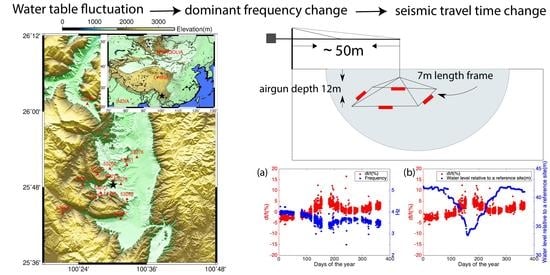
Impacts of Reservoir Water Level Fluctuation on Measuring Seasonal Seismic Travel Time Changes in the Binchuan Basin, Yunnan, China


Abstract
:
1. Introduction
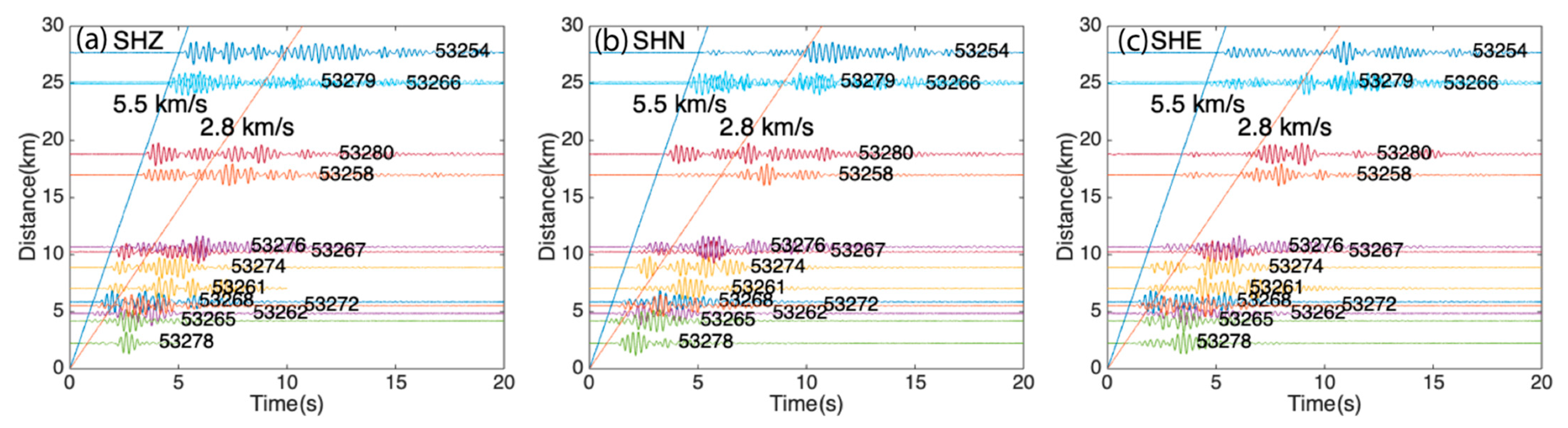
2. Airgun Data
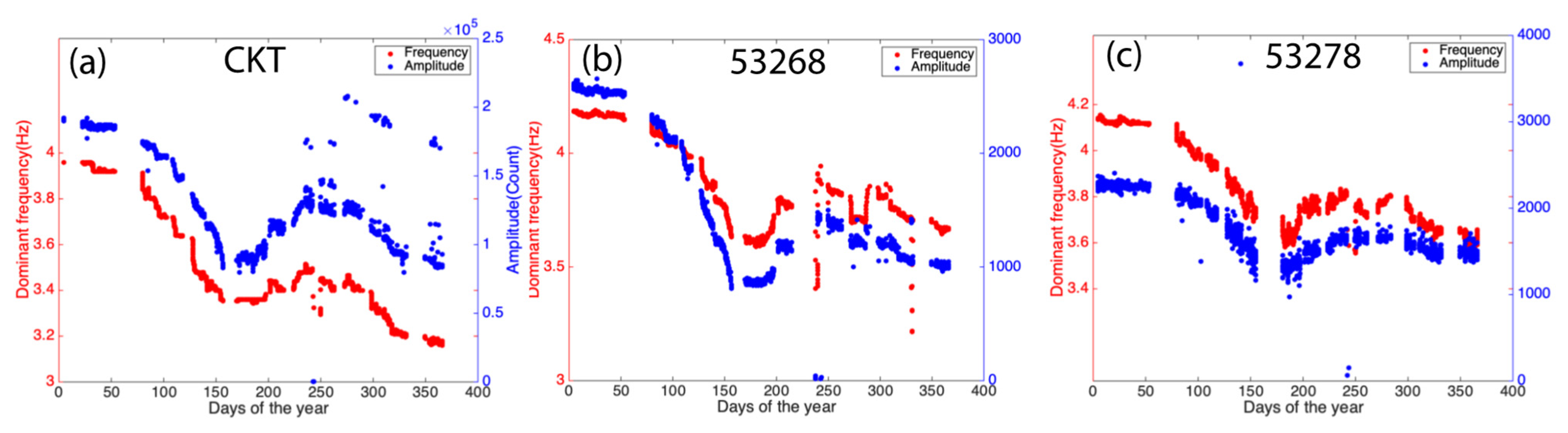
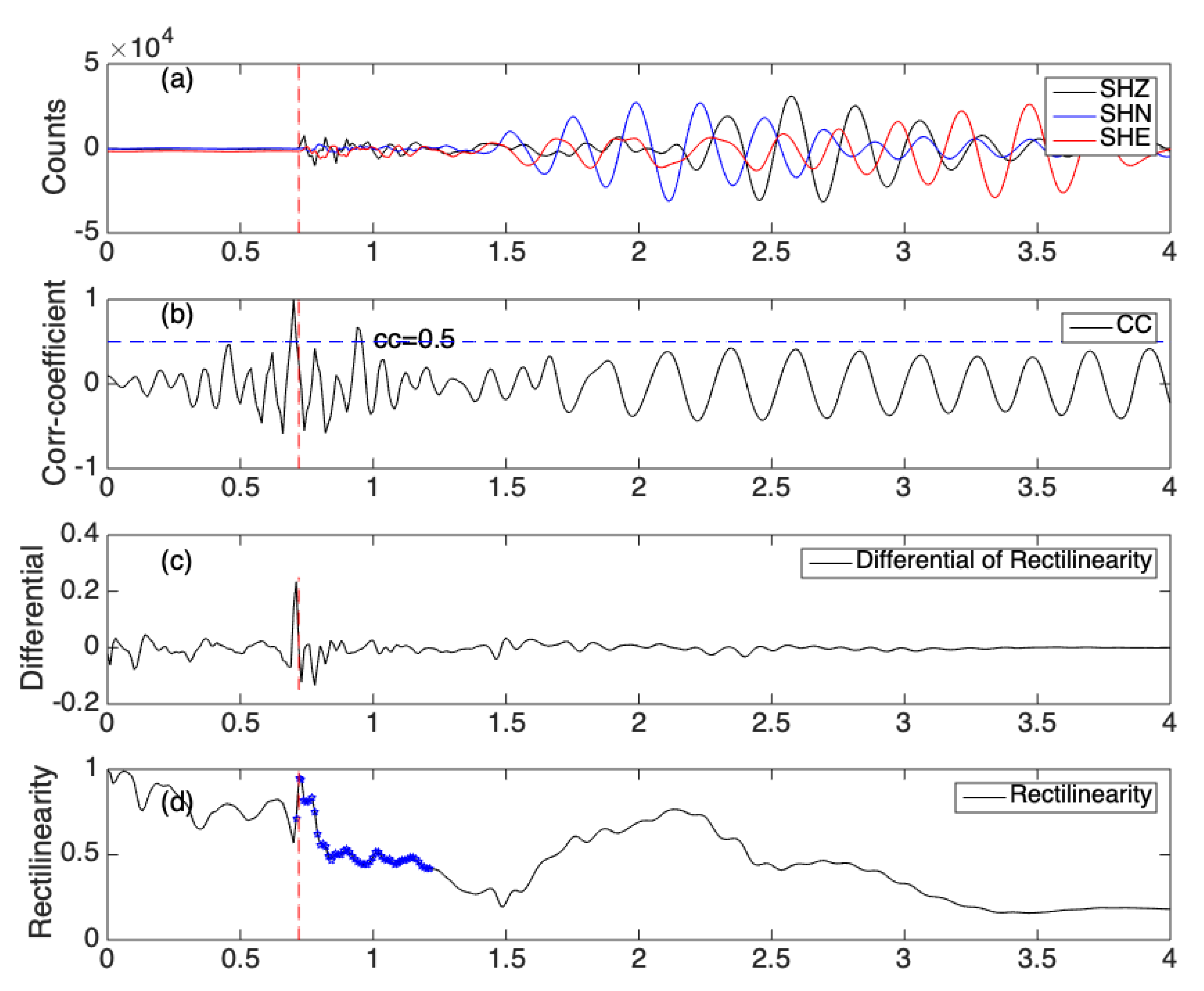
2.1. Source Characteristics
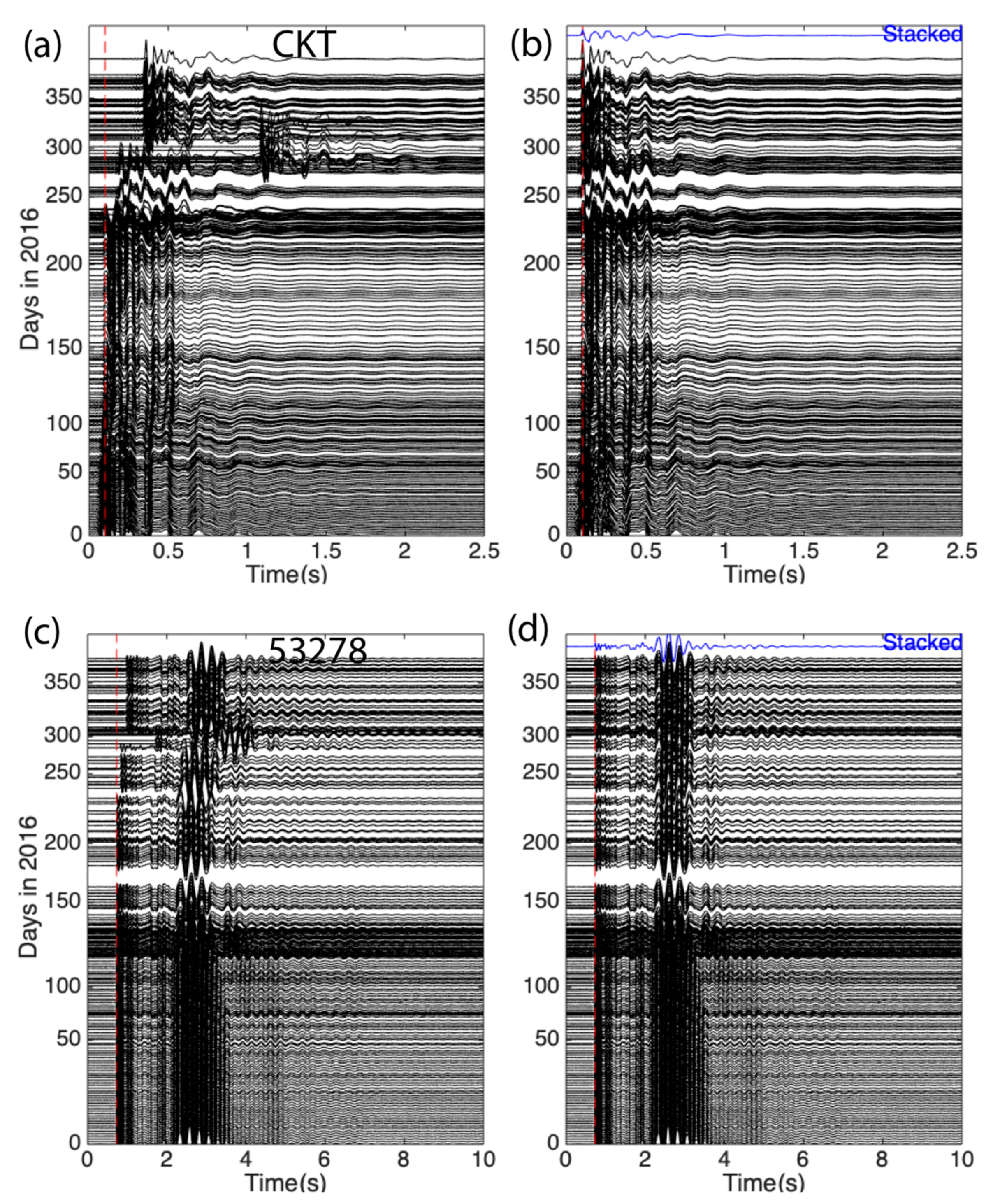
2.2. Airgun Data Quality
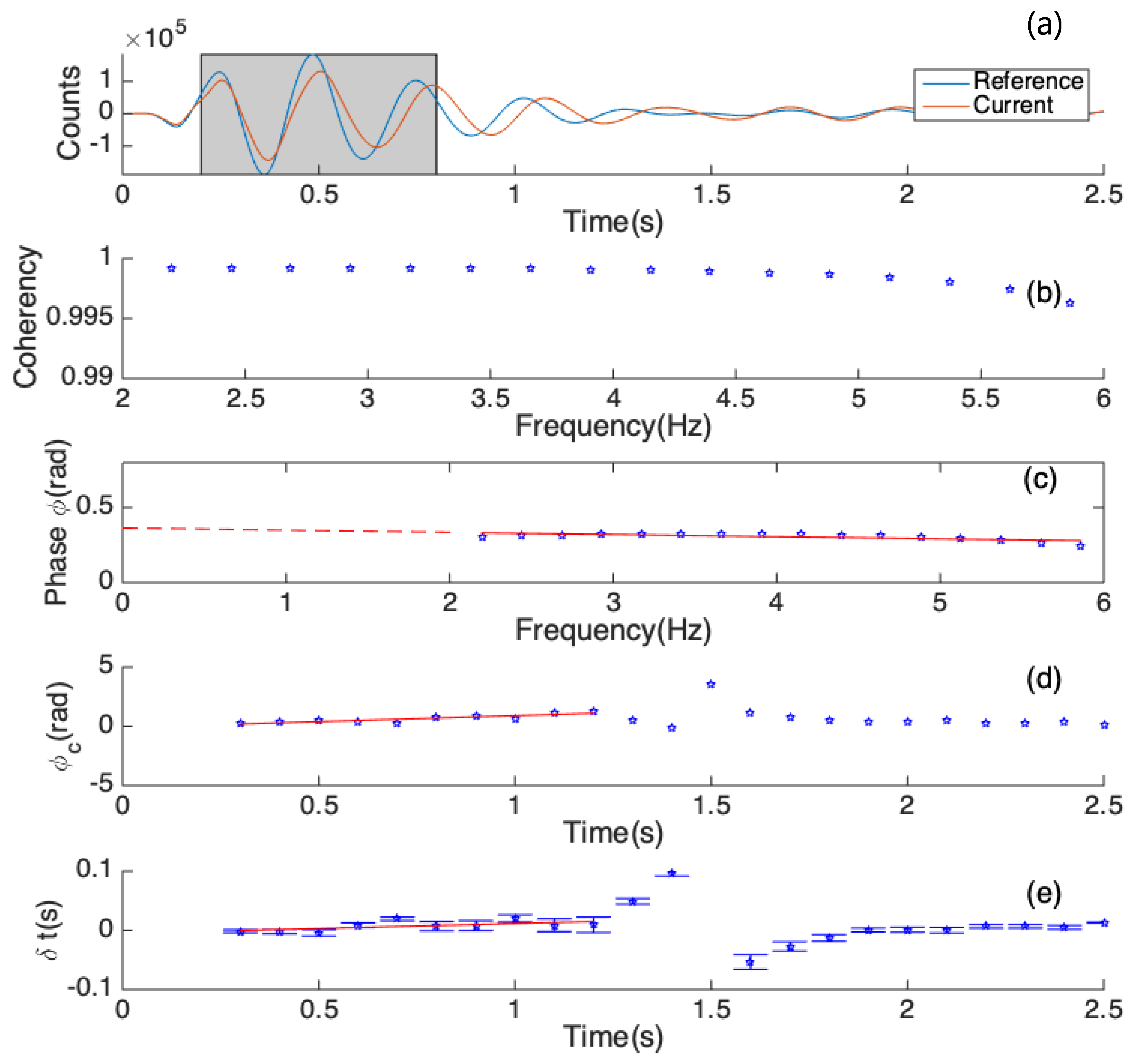
3. A Modified Moving-Window Cross-Spectrum method
4. Results
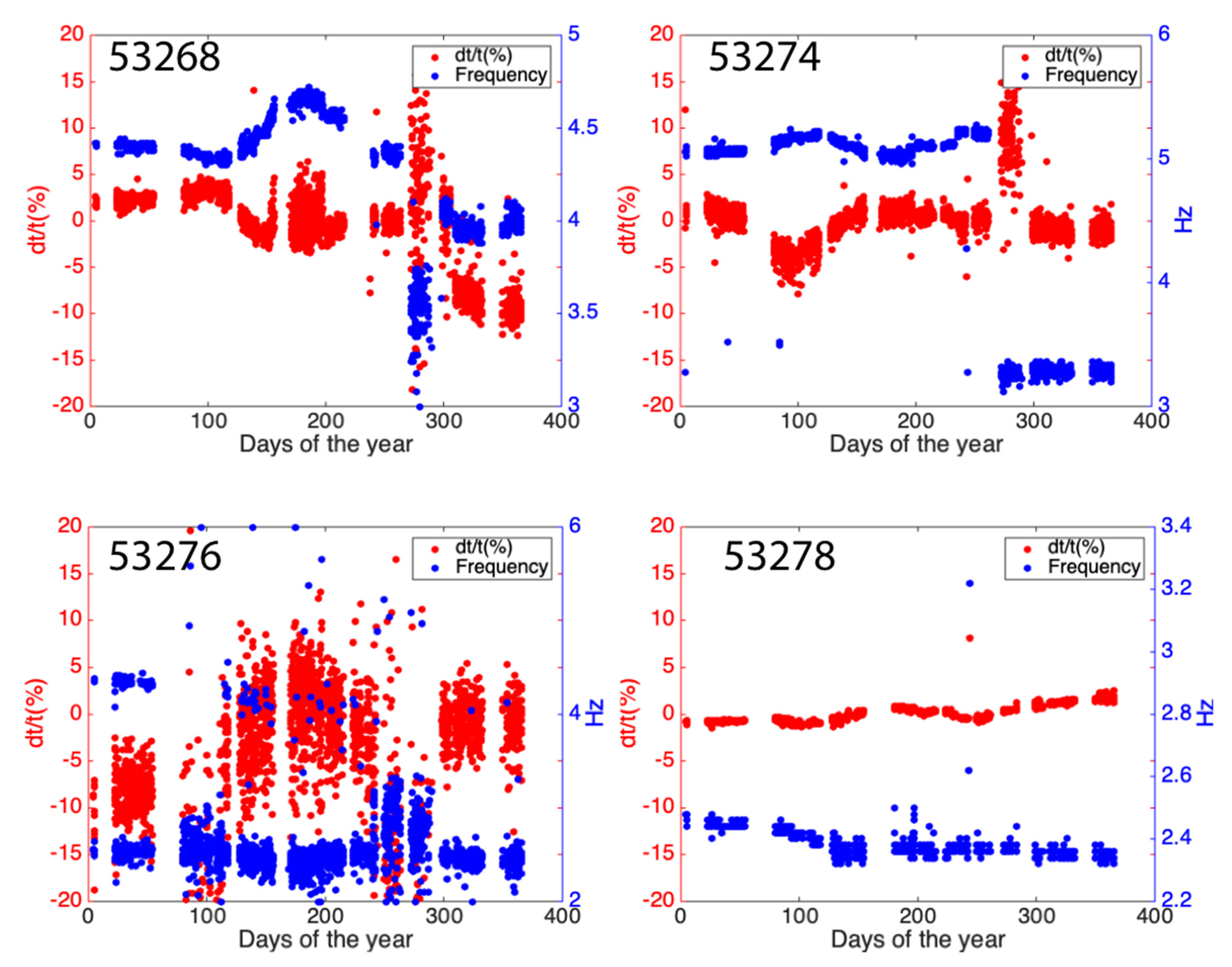
4.1. δt/t Derived Directly from Corrected Airgun Waveforms
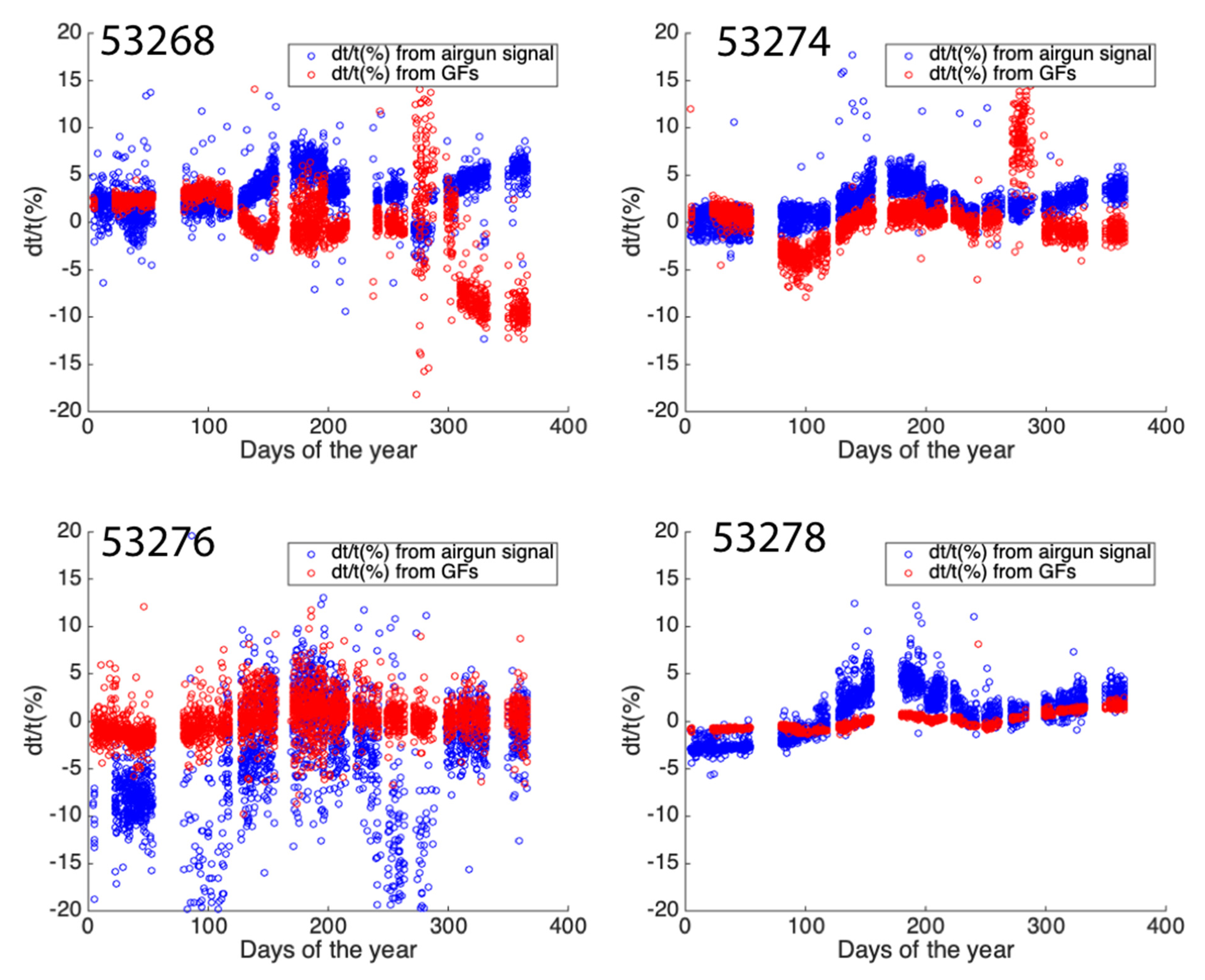
4.2. δt/t Derived after Deconvolution of the CKT Waveform
5. Discussion
5.1. The Magnitude of Change from Airgun
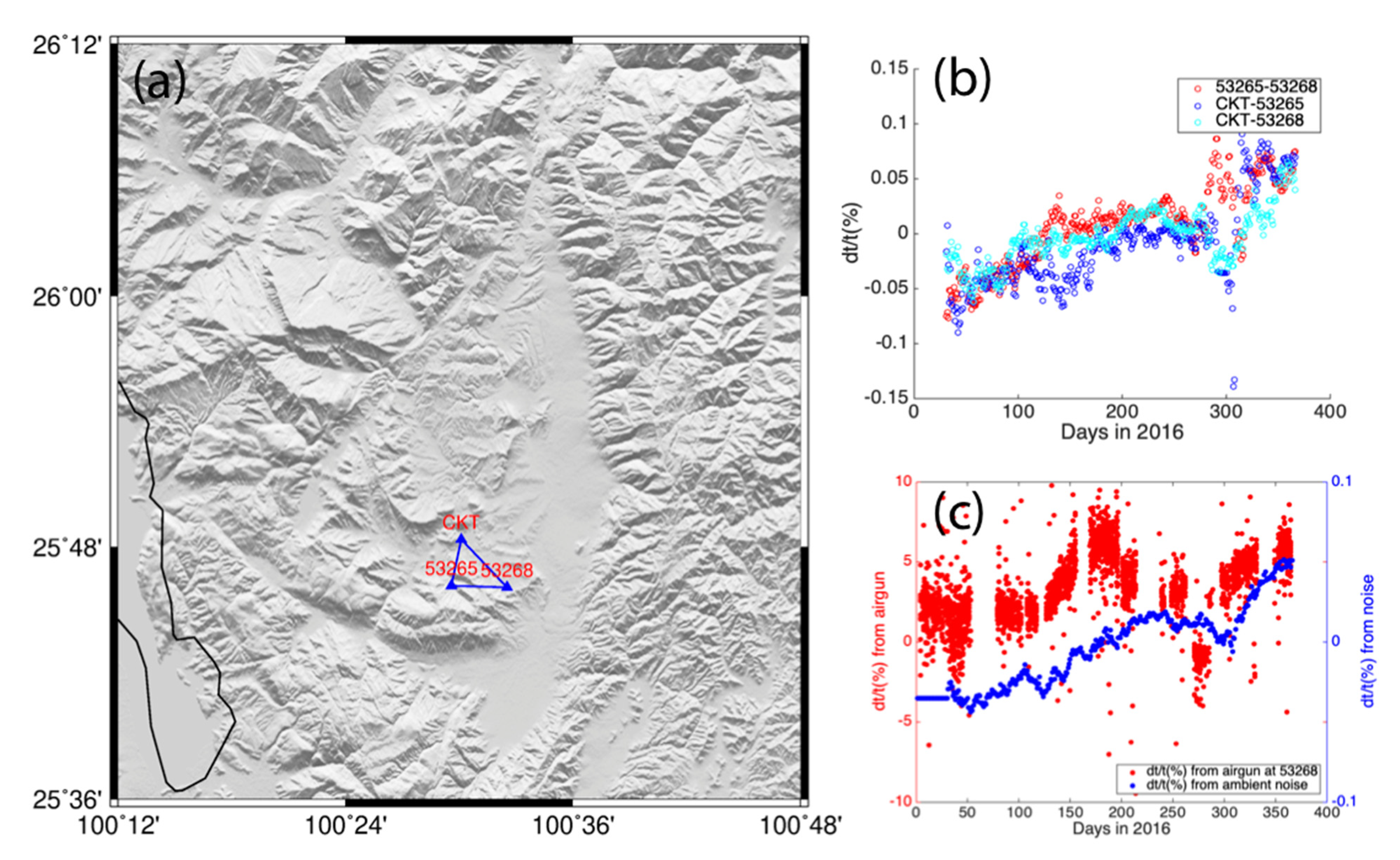
5.2. δt/t from Ambient Noise
5.3. Possible Mechanism of from Ambient Noise
5.4. Difference of from Ambient Noise and Airgun
5.5. Mechanism of Change from Airgun
6. Conclusions
Supplementary Materials
Author Contributions
Funding
Institutional Review Board Statement
Informed Consent Statement
Data Availability Statement
Acknowledgments
Conflicts of Interest
References
- Whitcomb, J.H.; Garmany, J.D.; Anderson, D.L. Earthquake prediction: Variation of seismic velocities before the San Francisco earthquake. Science 1973, 180, 632–635. [Google Scholar] [CrossRef] [PubMed]
- Rikitake, T. Earthquake precursors. Bull. Seismol. Soc. Am. 1975, 65, 1133–1162. [Google Scholar]
- Campillo, M.; Paul, A. Long-range correlations in the diffuse seismic coda. Science 2003, 299, 547–549. [Google Scholar] [CrossRef] [PubMed] [Green Version]
- Cicerone, R.D.; Ebel, J.E.; Britton, J. A systematic compilation of earthquake precursors. Tectonophysics 2009, 476, 371–396. [Google Scholar]
- Moro, M.; Saroli, M.; Stramondo, S.; Bignami, C.; Albano, M.; Falcucci, E.; Wegmüller, U. New insights into earthquake precursors from InSAR. Sci. Rep. 2017, 7, 1–11. [Google Scholar] [CrossRef] [PubMed] [Green Version]
- Brenguier, F.; Shapiro, N.M.; Campillo, M.; Ferrazzini, V.; Duputel, Z.; Coutant, O.; Nercessian, A. Towards forecasting volcanic eruptions using seismic noise. Nat. Geosci. 2008, 1, 126. [Google Scholar] [CrossRef] [Green Version]
- Wu, C.; Delorey, A.; Brenguier, F.; Hadziioannou, C.; Daub, E.G.; Johnson, P. Constraining depth range of s wave velocity decrease after large earthquakes near Parkfield, California. Geophys. Res. Lett. 2016, 43, 6129–6136. [Google Scholar] [CrossRef]
- Yang, H.; Duan, Y.; Song, J.; Wang, W.; Yang, W.; Tian, X.; Wang, B. Illuminating high-resolution crustal fault zones using multi-scale dense arrays and airgun source. Earthq. Res. Adv. 2021. [Google Scholar] [CrossRef]
- Duputel, Z.; Ferrazzini, V.; Brenguier, F.; Shapiro, N.; Campillo, M.; Nercessian, A. Real time monitoring of relative velocity changes using ambient seismic noise at the Piton de la Fournaise volcano (La Réunion) from January 2006 to June 2007. J. Volcanol. Geotherm. Res. 2009, 184, 164–173. [Google Scholar] [CrossRef]
- Lecocq, T.; Longuevergne, L.; Pedersen, H.A.; Brenguier, F.; Stammler, K. Monitoring ground water storage at mesoscale using seismic noise: 30 years of continuous observation and thermo-elastic and hydrological modeling. Sci. Rep. 2017, 7, 1–16. [Google Scholar] [CrossRef] [Green Version]
- Clements, T.; Denolle, M.A. Tracking groundwater levels using the ambient seismic field. Geophys. Res. Lett. 2018, 45, 6459–6465. [Google Scholar] [CrossRef] [Green Version]
- Liu, C.; Aslam, K.; Daub, E. Seismic velocity changes caused by water table fluctuation in the New Madrid seismic zone and Mississippi embayment. J. Geophys. Res. Solid Earth 2020, 125. [Google Scholar] [CrossRef]
- Silver, P.G.; Daley, T.M.; Niu, F.; Majer, E.L. Active source monitoring of cross-well seismic travel time for stress-induced changes. Bull. Seismol. Soc. Am. 2007, 97, 281–293. [Google Scholar] [CrossRef]
- Sens-Schönfelder, C.; Larose, E. Temporal changes in the lunar soil from correlation of diffuse vibrations. Phys. Rev. E 2008, 78, 045601. [Google Scholar] [CrossRef] [PubMed] [Green Version]
- Niu, F.; Silver, P.G.; Daley, T.M.; Cheng, X.; Majer, E.L. Preseismic velocity changes observed from active source monitoring at the Parkfield SAFOD drill site. Nature 2008, 454, 204. [Google Scholar] [CrossRef] [PubMed]
- Meier, U.; Shapiro, N.M.; Brenguier, F. Detecting seasonal variations in seismic velocities within Los Angeles basin from correlations of ambient seismic noise. Geophys. J. Int. 2010, 181, 985–996. [Google Scholar] [CrossRef] [Green Version]
- Hillers, G.; Retailleau, L.; Campillo, M.; Inbal, A.; Ampuero, J.-P.; Nishimura, T. In situ observations of velocity changes in response to tidal deformation from analysis of the high-frequency ambient wavefield. J. Geophys. Res. Solid Earth 2015, 120, 210–225. [Google Scholar] [CrossRef] [Green Version]
- Wang, B.; Yang, W.; Wang, W.; Yang, J.; Li, X.; Ye, B. Diurnal and semidiurnal P-and S-wave velocity changes measured using an airgun source. J. Geophys. Res. Solid Earth 2020, 125. [Google Scholar] [CrossRef]
- De Fazio, T.L.; Aki, K.; Alba, J. Solid earth tide and observed change in the in situ seismic velocity. J. Geophys. Res. 1973, 78, 1319–1322. [Google Scholar] [CrossRef]
- Yamamura, K.; Sano, O.; Utada, H.; Takei, Y.; Nakao, S.; Fukao, Y. Long-term observation of in situ seismic velocity and attenuation. J. Geophys. Res. 2003, 108, 2317. [Google Scholar] [CrossRef]
- Mao, S.; Campillo, M.; van der Hilst, R.D.; Brenguier, F.; Stehly, L.; Hillers, G. High temporal resolution monitoring of small variations in crustal strain by dense seismic arrays. Geophys. Res. Lett. 2019, 46, 128–137. [Google Scholar] [CrossRef] [Green Version]
- Li, Y.-G.; Chen, P.; Cochran, E.S.; Vidale, J.E.; Burdette, T. Seismic evidence for rock damage and healing on the San Andreas fault associated with the 2004 M 6.0 Parkfield earthquake. Bull. Seismol. Soc. Am. 2006, 96, S349–S363. [Google Scholar] [CrossRef]
- Li, Y.-G.; Vidale, J.E.; Aki, K.; Xu, F.; Burdette, T. Evidence of shallow fault zone strengthening after the 1992 M7. 5 Landers, California, earthquake. Science 1998, 279, 217–219. [Google Scholar] [CrossRef] [Green Version]
- Li, Y.-G.; Vidale, J.E.; Day, S.M.; Oglesby, D.D.; Cochran, E. Postseismic fault healing on the rupture zone of the 1999 M 7.1 Hector Mine, California, earthquake. Bull. Seismol. Soc. Am. 2003, 93, 854–869. [Google Scholar] [CrossRef]
- Nishimura, T.; Uchida, N.; Sato, H.; Ohtake, M.; Tanaka, S.; Hamaguchi, H. Temporal changes of the crustal structure associated with the M6.1 earthquake on September 3, 1998, and the volcanic activity of Mount Iwate, Japan. Geophys. Res. Lett. 2000, 27, 269–272. [Google Scholar] [CrossRef] [Green Version]
- Wang, B.; Zhu, P.; Chen, Y.; Niu, F.; Wang, B. Continuous subsurface velocity measurement with coda wave interferometry. J. Geophys. Res. Solid Earth 2008, 113. [Google Scholar] [CrossRef] [Green Version]
- Wegler, U.; Lühr, B.-G.; Snieder, R.; Ratdomopurbo, A. Increase of shear wave velocity before the 1998 eruption of Merapi volcano (Indonesia). Geophys. Res. Lett. 2006, 33, L09303. [Google Scholar] [CrossRef] [Green Version]
- Yang, W.; Wang, B.; Yuan, S.; Ge, H. Temporal variation of seismic-wave velocity associated with groundwater level observed by a downhole airgun near the Xiaojiang fault zone. Seismol. Res. Lett. 2018, 89, 1014–1022. [Google Scholar] [CrossRef]
- Peng, Z.; Ben-Zion, Y. Temporal changes of shallow seismic velocity around the Karadere-Düzce branch of the north Anatolian fault and strong ground motion. Pure Appl. Geophys. 2006, 163, 567–600. [Google Scholar] [CrossRef]
- Poupinet, G.; Ellsworth, W.L.; Frechet, J. Monitoring velocity variations in the crust using earthquake doublets: An application to the Calaveras Fault, California. J. Geophys. Res. 1984, 89, 5719–5731. [Google Scholar] [CrossRef] [Green Version]
- Rubinstein, J.L.; Beroza, G.C. Evidence for widespread nonlinear strong ground motion in the Mw 6.9 Loma Prieta earthquake. Bull. Seismol. Soc. Am. 2004, 94, 1595–1608. [Google Scholar] [CrossRef]
- Rubinstein, J.L.; Beroza, G.C. Nonlinear strong ground motion in the ML 5.4 Chittenden earthquake: Evidence that preexisting damage increases susceptibility to further damage. Geophys. Res. Lett. 2004, 31, L23614. [Google Scholar] [CrossRef]
- Rubinstein, J.L.; Uchida, N.; Beroza, G.C. Seismic velocity reductions caused by the 2003 Tokachi-Oki earthquake. J. Geophys. Res. 2007, 112, B05315. [Google Scholar] [CrossRef] [Green Version]
- Schaff, D.P.; Beroza, G.C. Coseismic and postseismic velocity changes measured by repeating earthquakes. J. Geophys. Res. 2004, 109, B10302. [Google Scholar] [CrossRef]
- Sens-Schönfelder, C.; Wegler, U. Passive image interferometry and seasonal variations of seismic velocities at Merapi Volcano, Indonesia. Geophys. Res. Lett. 2006, 33. [Google Scholar] [CrossRef]
- Chen, Y.; Wang, B.; Yao, H. Seismic airgun exploration of continental crust structures. Sci. China Earth Sci. 2017, 60, 1739–1751. [Google Scholar] [CrossRef]
- Wang, B.; Ge, H.; Yang, W.; Wang, W.; Wang, B.; Wu, G.; Su, Y. Transmitting seismic station monitors fault zone at depth. Eos Trans. Am. Geophys. Union 2012, 93, 49–50. [Google Scholar] [CrossRef]
- Wang, B.; Tian, X.; Zhang, Y.; Li, Y.; Yang, W.; Zhang, B.; Li, X. Seismic signature of an untuned large-volume airgun array fired in a water reservoir. Seismol. Res. Lett. 2018, 89, 983–991. [Google Scholar] [CrossRef]
- Yang, H.; Duan, Y.; Song, J.; Jiang, X.; Tian, X.; Yang, W.; Yang, J. Fine Structure of the Chenghai Fault Zone, Yunnan, China, Constrained from Teleseismic Travel Time and Ambient Noise Tomography. J. Geophys. Res. Solid Earth 2020, 125, e2020JB019565. [Google Scholar] [CrossRef]
- Zhang, Y.; Wang, B.; Lin, G.; Wang, W.; Yang, W.; Wu, Z. Upper crustal velocity structure of Binchuan, Yunan revealed by dense array local seismic tomography. Chin. J. Geophys. 2020, 63, 3292–3306. (In Chinese) [Google Scholar] [CrossRef]
- Liu, Z.; Su, Y.; Wang, B.; Wang, B.; Yang, J.; Li, X. Study on analysis method of travel time variations of seismic wave of active source in Binchuan. J. Seismol. Res. 2015, 38, 591–597. (In Chinese) [Google Scholar]
- Chen, J.; Ye, B.; Gao, Q.; Wang, J.; Li, X.; Yang, J. Study on travel time variation of the wave from large volume air-gun source before and after 2016 Yunlong Ms 5.0 earthquake. J. Seismol. Res. 2017, 40, 550–557. (In Chinese) [Google Scholar]
- Zhou, Q.; Chen, J. Influence of different triggering conditions of airgun source on travel time changes. J. Seismol. Res. 2018, 41, 264–272. [Google Scholar]
- Xiang, Y.; Yang, R.; Wang, B.; Zhou, Y.; Lu, Y.; Wu, H.; Junwei, Q.I.; Peng, J. Study on the Influence of Airgun Excitation Conditions on Airgun Signals and Travel Time Variation Measurements. Earthq. Res. China 2019, 33, 336–353. [Google Scholar] [CrossRef]
- Wang, M.; Shen, Z.K. Present-day crustal deformation of continental China derived from GPS and its tectonic implications. J. Geophys. Res. Solid Earth 2020, 125, e2019JB018774. [Google Scholar] [CrossRef] [Green Version]
- Zhou, Q.; Guo, S.; Xiang, H. Principle and method of delineation of potential seismic sources in northeastern Yunnan province. Seismol. Geol. 2004, 26, 761–771. [Google Scholar]
- Wang, B.; Wu, G.; Su, Y.; Wang, B.; Ge, H.; Jin, M. Site construction of the Binchuan transmitting seismic stations and preliminary observational data. J. Seismol. Res. 2015, 38, 1–6. [Google Scholar]
- Huang, X.; Wu, Z.; Li, J.; Nima, C.; Liu, Y.; Huang, X.; Zhang, D. Tectonic geomorphology and Quaternary tectonic activity in the northwest Yunnan rift zone. Geol. Bull. China 2014, 3, 578–593. [Google Scholar]
- Luan, Y.; Yang, H.; Wang, B. Large volume air-gun waveform data processing (I): Binchuan, Yunnan. Earthq. Res. China 2016, 32, 305–318. [Google Scholar]
- Xia, J.; Jin, X.; Cai, H.; Xu, J. The time-frequency characteristic of a large volume airgun source wavelet and its influencing factors. Earthq. Res. China 2016, 30, 364–379. [Google Scholar]
- McNamara, D.E.; Buland, R.P. Ambient noise levels in the continental United States. Bull. Seismol. Soc. Am. 2004, 94, 1517–1527. [Google Scholar] [CrossRef]
- Aster, R.C.; McNamara, D.E.; Bromirski, P.D. Multidecadal climate-induced variability in microseisms. Seismol. Res. Lett. 2008, 79, 194–202. [Google Scholar] [CrossRef]
- Zhan, Z.; Tsai, V.C.; Clayton, R.W. Spurious velocity changes caused by temporal variations in ambient noise frequency content. Geophys. J. Int. 2013, 194, 1574–1581. [Google Scholar] [CrossRef] [Green Version]
- Vidale, J.E. Complex polarization analysis of particle motion. Bull. Seismol. Soc. Am. 1986, 76, 1393–1405. [Google Scholar]
- Samson, J.C.; Olson, J.V. Some comments on the descriptions of the polarization states of waves. Geophys. J. Int. 1980, 61, 115–129. [Google Scholar] [CrossRef] [Green Version]
- Bataille, K.; Chiu, J.M. Polarization analysis of high-frequency, three-component seismic data. Bull. Seismol. Soc. Am. 1991, 81, 622–642. [Google Scholar]
- Clarke, D.; Zaccarelli, L.; Shapiro, N.M.; Brenguier, F. Assessment of resolution and accuracy of the Moving Window Cross Spectral technique for monitoring crustal temporal variations using ambient seismic noise. Geophys. J. Int. 2011, 186, 867–882. [Google Scholar] [CrossRef]
- Mordret, A.; Mikesell, T.D.; Harig, C.; Lipovsky, B.P.; Prieto, G.A. Monitoring southwest Greenland’s ice sheet melt with ambient seismic noise. Sci. Adv. 2016, 2, 1–9. [Google Scholar] [CrossRef] [Green Version]
- Wang, Q.-Y.; Brenguier, F.; Campillo, M.; Lecointre, A.; Takeda, T.; Aoki, Y. Seasonal crustal seismic velocity changes throughout Japan. J. Geophys. Res. Solid Earth 2017, 122, 7987–8002. [Google Scholar] [CrossRef]
- Langston, C.A. Structure under Mount Rainier, Washington, inferred from teleseismic body waves. J. Geophys. Res. Solid Earth 1979, 84, 4749–4762. [Google Scholar] [CrossRef] [Green Version]
- Pei, S.; Niu, F.; Ben-Zion, Y.; Sun, Q.; Liu, Y.; Xue, X. Recovery due to earthquakes on the Longmenshan fault. Nat. Geosci. 2019, 12, 387–392. [Google Scholar] [CrossRef]
- Lecocq, T.; Caudron, C.; Brenguier, F. MSNoise, a python package for monitoring seismic velocity changes using ambient seismic noise. Seismol. Res. Lett. 2014, 85, 715–726. [Google Scholar] [CrossRef] [Green Version]
- Talwani, P.; Chen, L.; Gahalaut, K. Seismogenic permeability, ks. J. Geophys. Res. Solid Earth 2007, 112, B07309. [Google Scholar] [CrossRef]
- Rivet, D.; Brenguier, F.; Cappa, F. Improved detection of preeruptive seismic velocity drops at the Piton de la Fournaise volcano. Geophys. Res. Lett. 2015, 42, 6332–6339. [Google Scholar] [CrossRef] [Green Version]
- Yu, W.; Yang, X.; Yu, J.; Sun, D. Temporal variations of surface wave amplitude in the data collected from Hutubi, Xinjiang airgun experiment. J. Seismol. Res. 2021, 44, 23–33. [Google Scholar]


Publisher’s Note: MDPI stays neutral with regard to jurisdictional claims in published maps and institutional affiliations. |
© 2021 by the authors. Licensee MDPI, Basel, Switzerland. This article is an open access article distributed under the terms and conditions of the Creative Commons Attribution (CC BY) license (https://creativecommons.org/licenses/by/4.0/).
Share and Cite
Liu, C.; Yang, H.; Wang, B.; Yang, J. Impacts of Reservoir Water Level Fluctuation on Measuring Seasonal Seismic Travel Time Changes in the Binchuan Basin, Yunnan, China. Remote Sens. 2021, 13, 2421. https://0-doi-org.brum.beds.ac.uk/10.3390/rs13122421
Liu C, Yang H, Wang B, Yang J. Impacts of Reservoir Water Level Fluctuation on Measuring Seasonal Seismic Travel Time Changes in the Binchuan Basin, Yunnan, China. Remote Sensing. 2021; 13(12):2421. https://0-doi-org.brum.beds.ac.uk/10.3390/rs13122421
Chicago/Turabian StyleLiu, Chunyu, Hongfeng Yang, Baoshan Wang, and Jun Yang. 2021. "Impacts of Reservoir Water Level Fluctuation on Measuring Seasonal Seismic Travel Time Changes in the Binchuan Basin, Yunnan, China" Remote Sensing 13, no. 12: 2421. https://0-doi-org.brum.beds.ac.uk/10.3390/rs13122421