
Remote Hyperspectral Imaging Acquisition and Characterization for Marine Litter Detection


1
INESCTEC—Institute for Systems and Computer Engineering, Technology and Science, Rua Dr. Roberto Frias, 4200-465 Porto, Portugal
2
ISEP—School of Engineering, Polytechnic Institute of Porto, Rua Dr. António Bernardino de Almeida 431, 4249-015 Porto, Portugal
*
Author to whom correspondence should be addressed.
Remote Sens. 2021, 13(13), 2536; https://0-doi-org.brum.beds.ac.uk/10.3390/rs13132536
Submission received: 4 May 2021
/
Revised: 15 June 2021
/
Accepted: 23 June 2021
/
Published: 29 June 2021
(This article belongs to the Special Issue Recent Advances in Hyperspectral Image Processing)
Abstract
:This paper addresses the development of a remote hyperspectral imaging system for detection and characterization of marine litter concentrations in an oceanic environment. The work performed in this paper is the following: (i) an in-situ characterization was conducted in an outdoor laboratory environment with the hyperspectral imaging system to obtain the spatial and spectral response of a batch of marine litter samples; (ii) a real dataset hyperspectral image acquisition was performed using manned and unmanned aerial platforms, of artificial targets composed of the material analyzed in the laboratory; (iii) comparison of the results (spatial and spectral response) obtained in laboratory conditions with the remote observation data acquired during the dataset flights; (iv) implementation of two different supervised machine learning methods, namely Random Forest (RF) and Support Vector Machines (SVM), for marine litter artificial target detection based on previous training. Obtained results show a marine litter automated detection capability with a 70–80% precision rate of detection in all three targets, compared to ground-truth pixels, as well as recall rates over 50%.
1. Introduction
Large marine litter accumulation zones, such as marine litter windrows [1], are appearing in the oceans, such as Atlantic [2] and Pacific [3,4]. Unfortunately, marine litter is an ever-increasing ecological problem that poses an imminent threat to marine ecosystems and ultimately even to humans, given it eventually inevitably enters the human food chain [5]. Therefore, marine stakeholders and research communities are now working on active/passive systems for detecting and/or capturing marine litter debris. An important research vector is in the detection and monitoring of the marine litter accumulation zones. Since the marine litter accumulation zones are spread over large areas, Earth observation satellite-based technological resources are currently being employed to detect and monitor marine litter. However, these efforts are still in the early stage of their development and still require further experimental validation, using complementary detection solutions, whether using remote and/or in-situ observations.
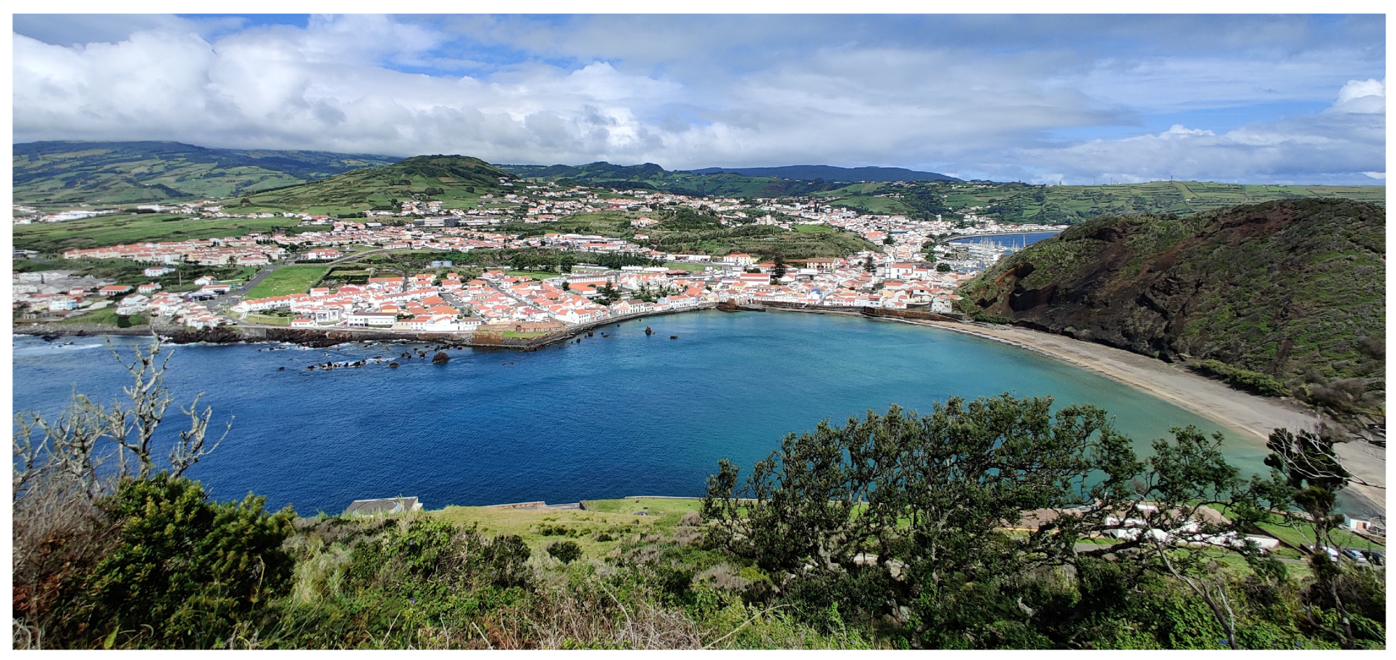
The work presented in this paper, contributes to the ongoing research efforts to develop new perception methodologies for marine litter detection. We present a remote hyperspectral imaging system that can detect marine litter and characterize the spectral information from marine litter samples, acquired in Pim Bay Area in Faial Island Azores, see Figure 1. This location is known to be a hotspot for marine litter concentration, see [6,7], and significant scientific work is currently devoted to studying the marine litter accumulation effects in that region.
For performing this spectral analysis of marine litter samples, the work carried out was divided into three phases, namely: (i) analyzing the marine litter samples in an outdoor setup using an hyperspectral image acquisition system that is able to acquire data from each marine litter sample, from visible (VIS) to SWIR wavelength range (400–2500 nm), thus determining the spectral response of each sample in that wavelength interval; (ii) to mount the same payload in two different aerial platforms (manned and unmanned) and perform remote data acquisition flights at different altitudes over artificial targets that were built using the same marine litter materials, (iii) develop, train and evaluate a model for the detection of different plastic types using machine learning methods: Random forests (RF) and Support Vector Machines (SVM).
This paper is organized as follows: Section 2 provides an overview of the related work in the detection of marine litter, with a particular focus on the current state-of-the-art using satellite and airborne solutions. Section 3 describes the hyperspectral imaging acquisition setup, also encompassing the different tests setups to acquire the hyperspectral data. Section 4 details the laboratory tests results and the dataset campaign. The remote manned and unmanned spectral characterization results and comparison with the results obtained in the laboratory environment can be found in Appendix A. Section 5 shows the experimental results obtained using RF and SVM methods implementations. Finally, Section 6 draws some conclusions on the work carried out and describes future work.
2. Related Work
2.1. Marine Litter Concentrations
Marine litter concentrations can be traced back to widely different sources. The source can be caused by professional and domestic activities, and can be intentional or not. Some of the actors typically mentioned concerning ocean pollution include not only the general public consumer attitude but also other activities ranging from coastal tourism and recreation to waste management policy in beaches. Economic activities usually installed in near-shore locations such as fisheries or aquaculture explorations are also commonly cited as potential sources, as well as harbors and other ship docking infrastructure [8].
Is possible to classify the marine litter samples according to their size [9]:
- Small microplastic: <1 mm;
- Large microplastic: 1–5 mm;
- Mesoplastic: 5.1–25 mm;
- Macroplastic: >25 mm.
The effect of ocean currents and harsh meteorological conditions such as direct exposure to UV light during extended periods [10], can alter the marine litter physical characteristics. Marine debris tend to deteriorate and break apart, turning macroplastics samples into microplastics and submerging from the sea surface, entering the water column [11], or resting in the seabed mainly due to biofouling. The taxonomy adopted for classification of marine litter samples is important for two main reasons:
- To understand the sinking and fouling of marine litter samples. Small plastic items start sinking sooner than larger plastic items, while larger debris will float for more time. This is due to the relation of buoyancy with item volume. Biofouling can also increase the density of the marine litter to the point where the debris sinks, see [12];
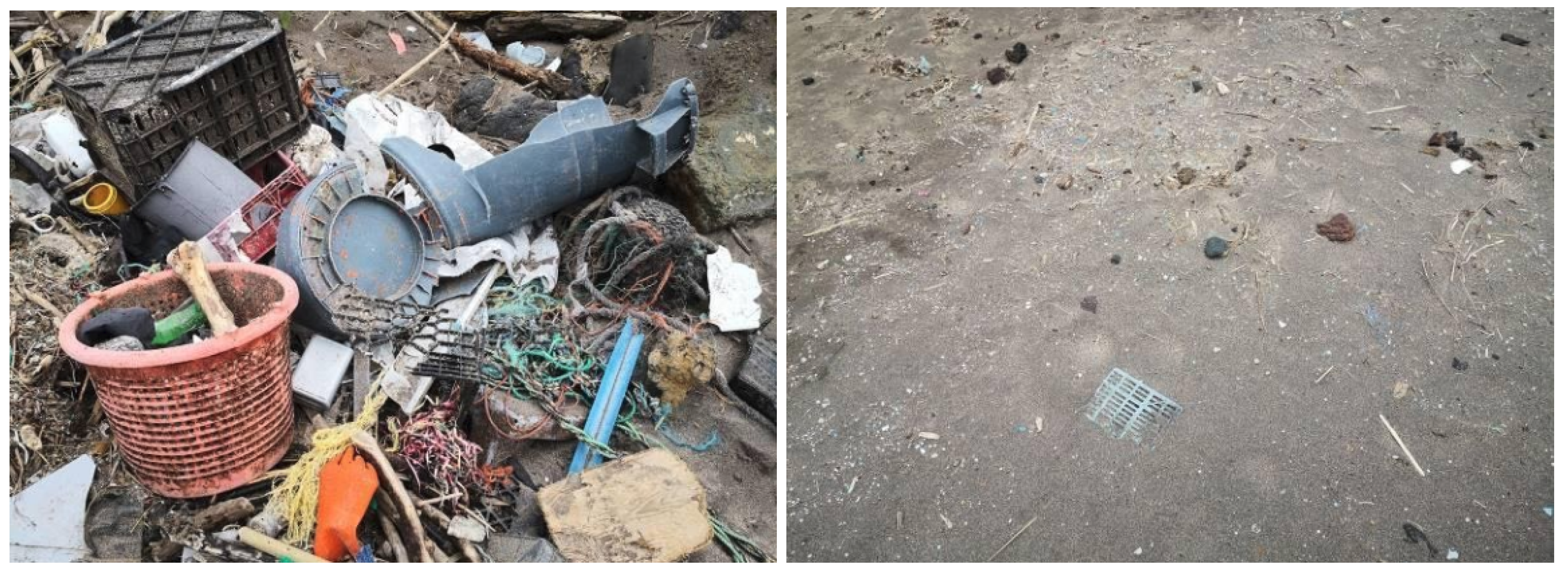
This is of fundamental importance since marine litter composition raises major concerns about the plastics contamination in the ocean, due to their chemically engineered durability, which decreases their bio-degradation rate [17]. The marine litter composition will increase the life span of these synthetic polymers which will stay on the ocean for longer [18], thus producing irreversible damage to the marine ecosystem. There are multiple examples of environmental impacts of marine debris [19], including entanglement of marine fauna, ingestion by seabirds or fish [20], as well as the possible dispersion of microbial and colonizing species to non-native waters [21,22]. Figure 2 shows marine litter found at the test site in Porto Pim bay (Faial Island, Azores).
2.2. Remote Marine Litter Detection
There are several applications for remote sensing in coastal areas [23]. However, this section focuses on remote marine litter detection. A summary of previous work on marine litter detection is presented in Table 1, focusing on previous research that conducted tests in real environment conditions. The table describes the related work considering the following items: types of sensor used to detect the marine litter, test site location, platform, target objects (marine litter samples) and developed algorithms.
Briefly summing up the table content, most of the previous work is being carried out using drones equipped with RGB cameras [24,25,26,27]. All these works resort to deep learning algorithms, such as Convolutional Neural Networks (CNN). Although the use of RGB cameras can be considered an easy and low-cost solution, it has operational constraints for detection such as water reflections due to sunglare, difficulty to achieve the required image resolution for the marine litter detection, and recent literature results seem to be shying away from visual-only systems as they are not the most suitable for extended coverage of the ocean. Other works result from NASA initiatives, such as the one that uses AVIRIS [28], which is an airborne solution provided by NASA. In [28], the authors first performed an in-situ analysis of dry and wet marine-harvested microplastics, to detect the absorption bands of each sample on the spectral wavelength to apply to the collected AVIRIS data.
Other authors based their solutions on the use of satellite data, such as satellite WorldView 3 (WV3) for marine litter detection [29]. In this work, in addition to the data collection with the satellite WV3, the authors also collected some samples from the test site that was subject to extensive laboratory analysis. To perform the atmospheric correction in the WV3 data it was used the Atmospheric Compensation algorithm from DigitalGlobe. The results were convolved using the RSRCalculator, which allowed to estimate the Anthropogenic Marine Debris (AMD) reflectance values for each spectral bands that afterward were compared to the laboratory results. The convolved spectral signatures were then used to train automated classification algorithms such as Support Vector Machine (SVM), Random Forest (RF) and Linear Discriminant Analysis (LDA). The results showed a precision of 80% in general (considering all algorithms applied). However, this precision is only to distinguish between mixture AMD and expanded polystyrene AMD.
Three other studies use the Sentinel 2 to detect marine litter [30,31,32]. Two studies use artificial targets, while one of them also uses plastic aggregations that were present in the test site. The usage of artificial targets is mainly due to being able to cover the spatial resolution of the multispectral sensor included in the satellite (which has a spatial resolution of 10 m × 10 m). However, in addition to the unsuitable spatial resolution for marine litter detection, the Sentinel-2 multispectral sensor also has a small number of spectral bands. In [30], the Sentinel-2A data atmospheric correction was performed using the ACOLITE and Sen2Cor algorithms. The authors also provide a comparison between the pixel coverage for each target. However, they do not perform any automated classification task. In work developed in [31], the authors use both Sentinel-2B and airborne data. For the airborne data, they compared three different algorithms: ENVI true color composite, greyscale HI index and greyscale NDHI index. The test was conducted only with beach targets and the authors did not perform any automated classification task. In [32], the authors developed the FDI algorithm, a new index created especially for Sentinel-2 data. This index allows easy and fast detection, and it also serves as input to the classification stage, using naive Bayes. The classification was performed between the following classes: water, seaweed, timber, plastic, foam and pumice. The results presented show 86% accuracy for “suspected plastics”, which do not identify the plastic-type.
A recent study [33] uses the PRISMA satellite data to perform tests with several pansharpening methods to improve the spatial resolution of the PRISMA hyperspectral sensor. The authors used several artificial targets with different sizes to test the possibility of using the PRISMA data for marine litter detection, and the minimum spatial resolution when using pansharpening methods. Although some plastic materials spectra are similar to the water spectra, the authors were able to produce marine plastic litter indexes, which had successfully detected the plastic targets placed in the test site.
Our proposed work follows the work already developed in [30,31,32], but extended to the use of a hyperspectral image system that collects data at different altitudes with a manned and unmanned aerial platforms, from 400 to 2500 nm. We characterize the target samples in wet and dry conditions to evaluate the influence of water in the marine litter spectral response. These samples were collected at the test site and used to construct targets according to the Sentinel 2 resolution. Furthermore, we extend previous work by developing, training, and testing supervised machine learning methods (RF, SVM) to detect and classify marine litter samples based on the remotely acquired hyperspectral flight data.

Table 1.
Marine litter detection state-of-the-art.
| Ref. | Sensor | Test Site | Satellite/Vehicle | Target Objects | Algorithms Used |
|---|---|---|---|---|---|
| [28] | (1) FTIR spectroscopy, (2) Airborne visible-infrared imaging spectrometer (AVIRIS) retrieved from the AVIRIS online data portal (224 bands between 360–2500 nm) | California Sunshine Canyon Landfill (USA) | AVIRIS | Plastic that was present in the test site | - Spectral similarity: Spectral contrast angle - Spectral mixing: used a simplified linear mixing simulation to analyze how spectral properties of the dry and wet marine-harvested microplastics were influenced by varying pixel coverage |
| [29] | (1) Laboratory: HyLogger 3 reflectance spectrometer system and APOGEE PS-300 (2) WorldView 3, using a multispectral with a spectral range from 397 to 2373 nm) | Chiloe Archipelago (northwestern area of Chilean Patagonia) | WorldView 3 | Plastic that was present in the test site | - Atmospheric correction of the WV3 data: Atmospheric Compensation from DigitalGlobe - The spectral collected using the WV3 were convolved using RSRCalculator to estimate the samples reflectance values for the spectral bands in order to compare with the spectral measurements from the laboratory |
| [30] | (1) S900 DJI Hexacopter: multispectral SLANTRANGE 3 P (S3 P), Parrot Sequoia multispectral (4 bands in the 450–850 nm), FLIR Duo R, and RGB camera (2) Sentinel-2A: multispectral camera (13 bands between 492–1376 nm) (3) Sentinel-1: Synthetic Aperture Radar | Tsamakia beach of Mytilene on Lesvos Island, Greece | - Drone - Sentinel-2A - Sentinel-1 | (i) plastic bottles (ii) plastic bags (iii) plastic fishing net Each one of these plastic types were held by a 10 m × 10 m frame | Atmospheric correction for the Sentinel-2A data: ACOLITE and Sen2Cor |
| [31] | (1) Sentinel-2B: Multispectral camera (13 bands between 492–1376 nm) (2) Airborne: Specim Asia Fenix (300–2500 nm) | Whitsand Bay (UK) | - Sentinel-2B - Airborne | (i) 2 plastic targets from NERC-FSF with colors grey and black (ii) 2 types of agricultural fleece plastic targets | Specim data analysis: ENVI true color composite, grey scale HI index and grey scale NDHI index |
| [32] | Sentinel 2A and 2B Multispectral sensors 13 bands between 492–1376 nm | Accra, Ghana Barbados, Caribbean Da Nang, Vietnam Late Island, Tonga Mytilene, Greece Gulf Islands, Canada Scotland, UK Durban, South Africa | - Sentinel 2A - Sentinel 2B | (i) Plastic aggregations that was present in the test site (ii) Deployed plastic targets | Acolyte to the correction phase, FDI to detect and Naive Bayes to classification stage |
| [24] | RGB Camera | Xabelia beach in Lesvos, Greece | DJI Phantom 4 Pro v2 | Plastic that was present in the test site | Deep learning algorithms - CNN (VGG16, VGG19, DenseNet121, DenseNet169, DenseNet201) |
| [25] | 20 MP RGB imaging sensor | Phnom Penh, Sihanoukville and Siem Reap in Cambodia | DJI Phantom 4 Pro v2 | Plastic that was present in the test site | APLASTIC-Q: (i) plastic litter detection (PLD-CNN) + (ii) plastic litter quantifier (PLQ-CNN) |
| [26,27] | 20 MP RGB imaging sensor | Cabedelo beach, Figueira da Foz, Portugal | DJI Phantom 4 Pro | Plastic that was present in the test site | - Random Forest - CNN |
| [33] | PRISMA hyperspectral, with 234 bands from 400–2500 nm and 30 m spatial resolution | Tsamakia beach, Lesvos Island, Greece | PRISMA satellite | 12 floating targets (5.1 m × 5.1 m, 2.4 m × 2.4 m, 0.6 m × 0.6 m), with HDPE, PET and PS | Pansharpening methods |
3. Hyperspectral Imaging System
This section describes the hyperspectral imaging system setup, including the description of the physical connections and their main components.
3.1. Hyperspectral Imaging System Setup
Concerning the hyperspectral imaging system setup, it consisted of a system composed of two pushbroom hyperspectral cameras [34], a CPU unit, GPS, and an inertial system. One of the hyperspectral cameras was a Specim FX10e, a GigE camera with a spectral range from 400 to 1000 nm wavelength and spatial resolution of 1024 pixels. The other camera was a HySpex Mjolnir S-620, a hyperspectral system composed of the hyperspectral camera, a data acquisition unit, GPS, a dedicated inertial system, a control board, power control and distribution, and an RGB camera, integrated into the same closed box. This hyperspectral camera has 620 pixels of spatial resolution and covers a spectral range from 1000 to 2500 nm wavelength. Table 2 depicts the main features of each hyperspectral camera.
In Figure 3 is possible to see the hyperspectral image system hardware architecture.
The hyperspectral imaging system in fact is dual and synchronized, since the Specim FX10e hyperspectral camera is triggered by the HySpex Mjolnir S-620 system. This trigger is related to INS/GPS (Applanix APX-15 UAV) for data georeference. Concerning the data acquisition, the HySpex system saves a HySpex file containing all the raw data collected by the camera. The data is processed after the flight with HySpex Rad software, which performs the calibration, and converts the raw data to radiance by removing the effects of the sensor in the raw data. For the SPECIM FX10e, the raw data is acquired using a customized data acquisition software (driver), and afterwards, the calibrated manufacturer gains are used to convert the raw data into radiance data.
3.2. Hyperspectral Imaging System Setup—Laboratory
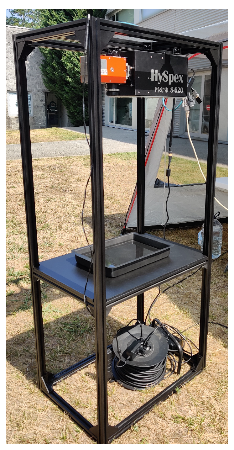
For conducting the tests, a laboratory setup with the cameras coupled together using a custom holder, was mounted to allow fixing the Specim FX10e camera to the HySpex system. The structure is shown in Figure 4. The distance between the cameras to the marine litter samples is 1 m in height.
The entire structure was built in black to minimize the sunlight reflections captured by the camera. In addition, the water placed in the tank is seawater collected in the Atlantic Ocean, the same ocean present in the test zone.
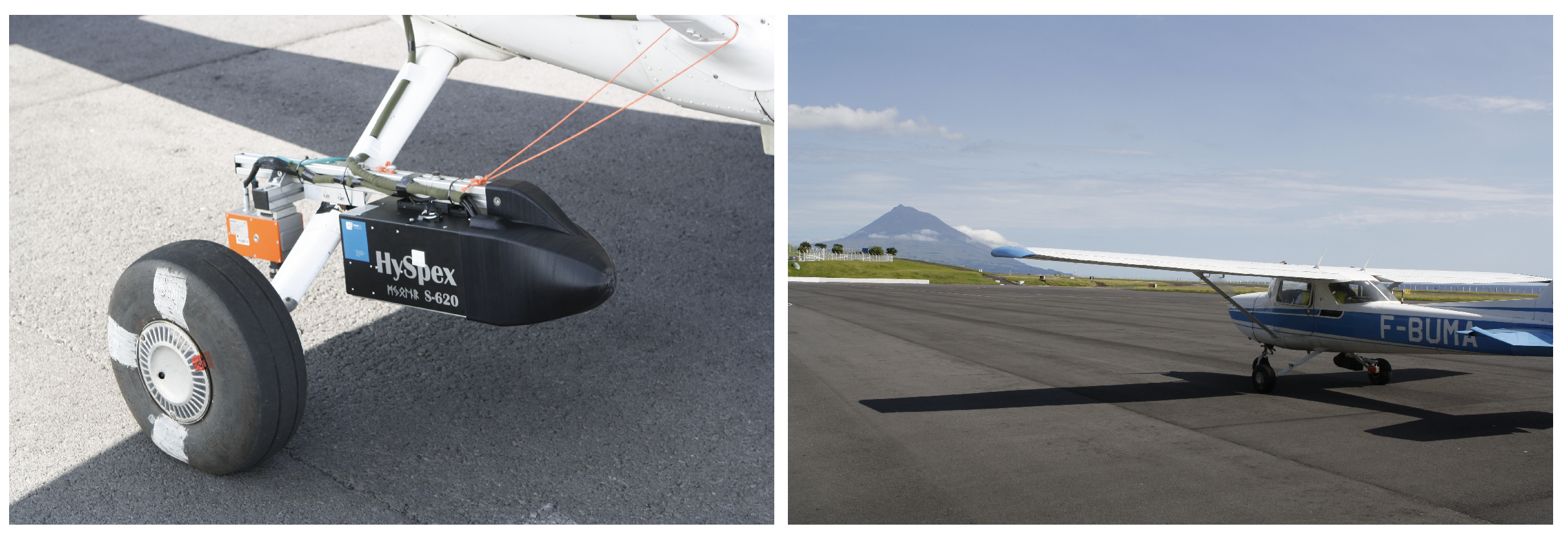
3.3. Hyperspectral Imaging System Setup—Manned Aircraft (F-BUMA)
The first aerial platform included in the project was a manned aircraft—A Cessna F150L. Figure 5 shows the system already assembled in the aircraft. The GPS antenna was placed in the rear window of the aircraft, inside the airplane and facing up. The system was built to ensure that lenses were at the same height, keeping the alignment between the cameras.
3.4. Hyperspectral Imaging System Setup—Unmanned Aircraft (Grifo-X)
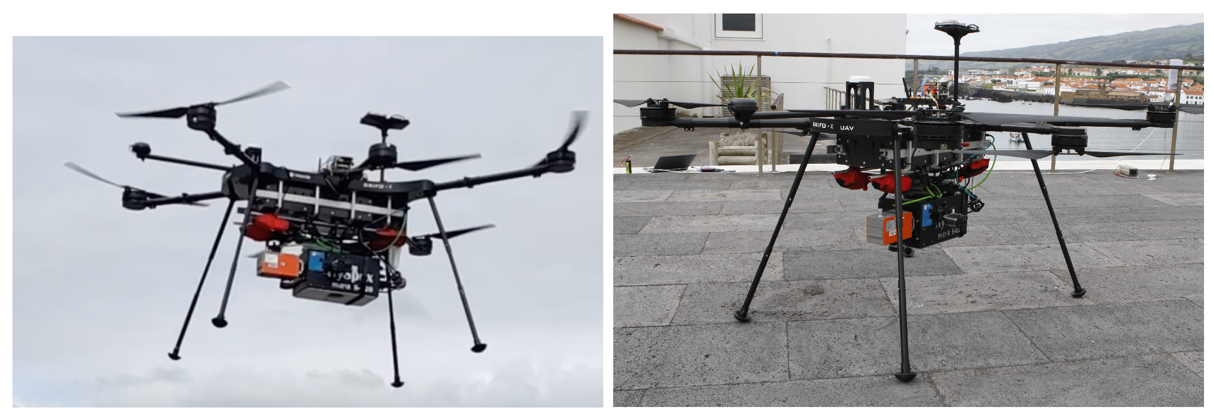
The second aerial platform included in the project was an unmanned aerial vehicle (UAV), Grifo-X, developed at CRAS (Center for Robotic and Autonomous System) from INESCTEC. The GPS antenna was installed in a custom support on top of the UAV frame. Figure 6 shows the hyperspectral imaging system mounted onto the Grifo-X UAV.
4. Laboratory Marine Litter Samples Characterization and Dataset Campaign
This section describes the laboratory tests to perform the marine litter samples characterization, and the dataset campaign realized in Porto Pim Bay, Faial Island, Azores.
4.1. Laboratory Marine Litter Samples Characterization
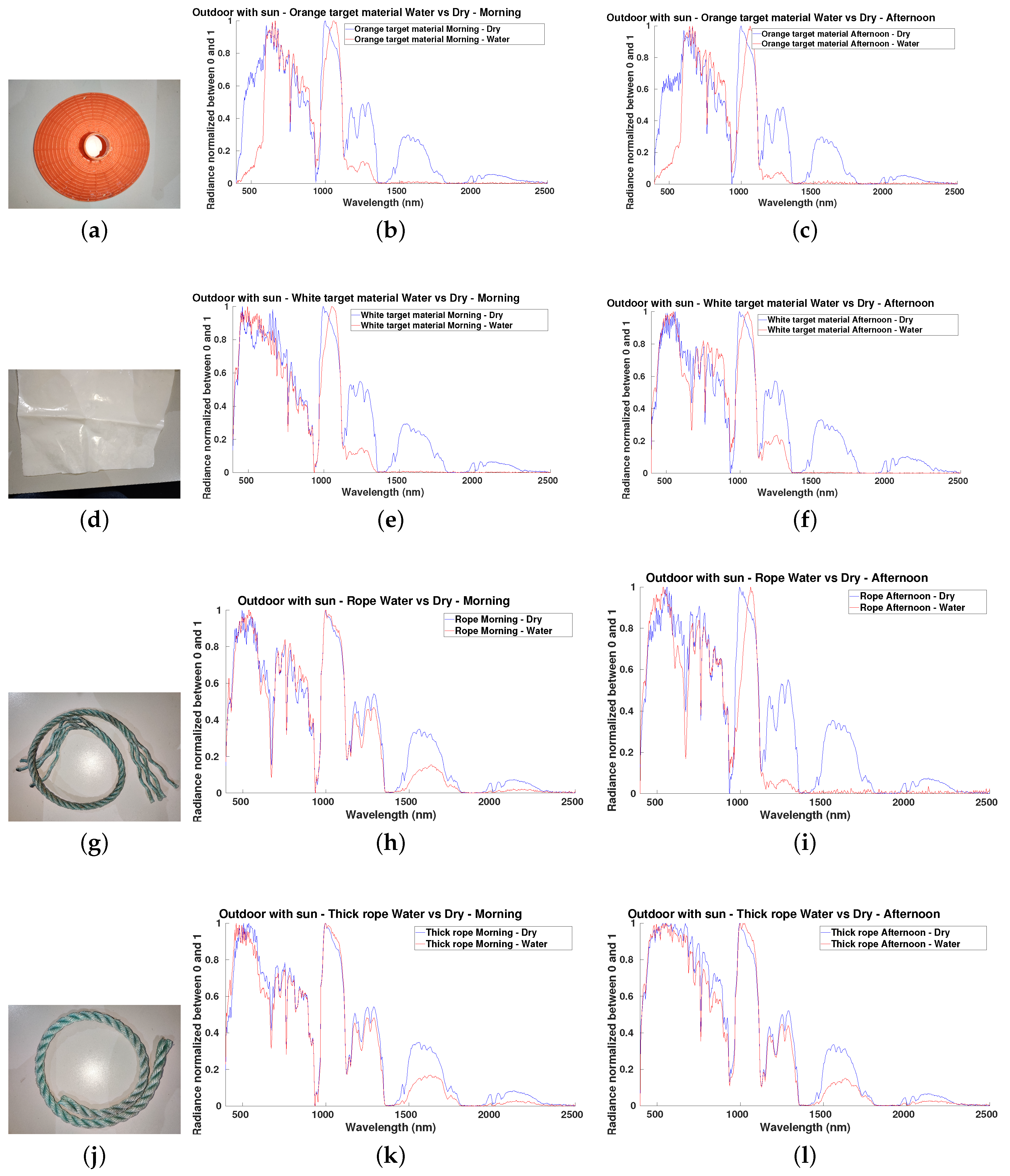
Before the flight campaigns, and to perform a ground-truth comparison of different marine litter samples, the hyperspectral imaging system was mounted in an outdoor environment as described in Section 3.2. The objective was to characterize the spectral response of the marine litter samples under direct sunlight, and under varying natural light conditions, i.e., morning and in the afternoon using dry and wet samples. This study will be helpful in future works to understand better the water effects, as well as the light incidence effects in the spectral analysis of the marine litter samples. The marine litter samples used in the test were identical to the ones used in the artificial targets on the airborne dataset campaigns, namely:
- Orange polypropylene plastic used for oyster aquaculture. This type of plastic is widely found in the hotspot analyzed, and can be observed in Figure 7a;
- Blue polypropylene ropes, used for fishery, one thin and another thick. This type of plastic is also widely found in the hotspot tested and can be observed in Figure 7g,j;
- White polyethylene plastic, used to cover greenhouses, see Figure 7d.
The results for both morning and afternoon tests of all target materials are shown in Figure 7. The results concerning the dry and wet samples are very similar, noticing an attenuation on the energy of the signal in the results of the wet samples due to water effects, but without significant variation in the absorption of spectral bands wavelength.
4.2. Dataset Campaign
The project dataset campaign occurred in Faial Island Azores from the 16th until the 25th of September of 2020. The artificial target setups were placed inside the Pim Bay area, for conducting the hyperspectral image data acquisition. In Figure 8 it is possible to see the location of three artificial targets, built using the marine litter samples, during the campaign. The targets dimension is 10 m × 10 m which corresponds to the minimal resolution (1 × 1 pixel) to be detected by Sentinel-2.
The flights were divided into two modules: manned fixed wing and unmanned flights. Each one of the aircrafts performed a flight a few moments before or after a flyby of the Sentinel-2 satellite. However, the data collected by Sentinel 2 on the flight’s days was not as good as expected due to cloud coverage. In our experimental setup, the cloud cover did not affect significantly the hyperspectral imaging system acquisition, as shown in Figure A5 (Appendix A) where is possible to see that the airplane, the UAV, and the laboratory setup produce similar results concerning the spectral profile of one of the targets. However, is know that cloud coverage affects hyperspectral data acquisition results and can reduce the amount of direct sunlight onto the targets, influencing the energy of the reflections and shifting absorption bands as described in more detail in [35].
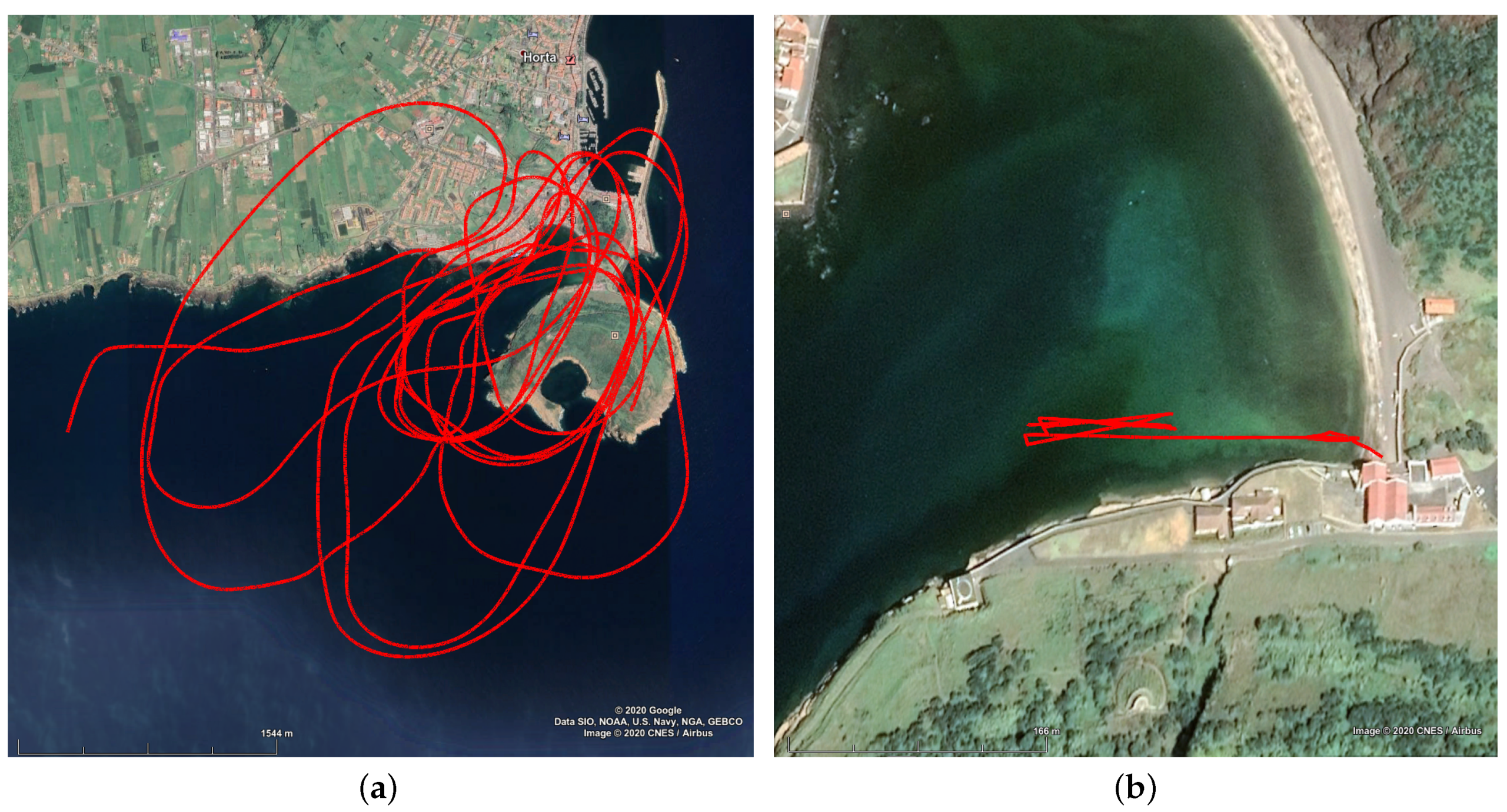
In Figure 9a is possible to see the trajectory of the F-BUMA aircraft during the 20 September 2020 flight, and in Figure 9b is possible to observe the smaller trajectory of the GRIFO-X UAV during the 25 September 2020 flight.
As a first approximation to characterize the obtained hyperspectral imaging data results, we compared the laboratory data with the flight data. To conduct this comparison, three different pixels from the three distinct targets were analyzed, namely a bright pixel, a medium intensity pixel and a dark pixel. The pixels were manually selected using the hyperspectral waterfall image (which is an “RGB” type of image using multiple spectral bands). In all analysis presented in this work, we did not use all the available flybys of the hyperspectral over the targets, but only the ones that contain all the three targets in the same flyby. The figures results can be found in Appendix A. It is possible to observe that the spectral response is similar but with attenuation on some of the spectral bands particularly in the visible 400–1000 nm wavelength. Another important feature is that the flight data matches the spectral response when compared with the laboratory data in each target, which is consistent with the fact that the targets use different plastics materials.
5. Target Detection and Classification
The characterization of the acquired hyperspectral imaging data is important. However, for helping solve the problem of marine litter detection and identification, automated means of detection need to be used to detect and classify marine litter in vast amount of data.
Therefore, in this work, we develop, train and compared the obtained results of two machine learning (ML) algorithms do detect and classify marine litter samples, namely: Random Forest (RF) [36] (RF) and Support Vector Machines (SVM) [37]. The algorithms were tested using the F-BUMA acquired data, due to time-consuming process of manual annotating the dataset for ground-truth and training purposes.
The training of the model was performed with data collected during the F-BUMA 18 September 2020 flight, which was divided to be used for training and fine tuning of the model parameters. The second flight, from 20 September 2020, was used for testing the results. This means that the model was trained using data from a different day than the one used for the prediction. The data was measured in raw units, and then transformed to radiance. This allows understanding of the possibility of having a hyperspectral imaging system in the future to detect marine litter concentrations in near real-time, which needs to be performed with radiance data.
Given the data characteristics, the flights were divided into flybys over the target (which considered only the data in the targets vicinity), and only the flybys with the three targets were used for training and prediction. In Table 3 is possible to observe some examples of the classes components. Table 4 and Table 5 show the pixel distribution for each class in each flyby. Class 1 represents the Orange target data, class 2 corresponds to the White target data and class 3 the Rope target data. Class 0 was created with all the remaining pixels, containing both land and water data. It was necessary to make this class to train the methods to recognize the characteristics of the non-marine litter pixels, by grouping all in one class.
To overcome some limitations in the training of the data. Some training techniques were adopted in the experiments, namely:
- Class imbalance: As can be observed in Table 4 and Table 5, the number of pixels for each class has a considerable variation. Some of the flybys do not hold information about all the classes, and the difference between the class 0 pixels and the other classes is significant. Therefore, we randomly selected some samples, so that the number of points is identical for each class. This was required, so the class with the highest number of points does not become dominant leading to overfitting;
- Feature normalization: Given the characteristics of the hyperspectral data that is affected by the variability of atmospheric conditions, particularly direct sunlight, it is necessary to carry out its normalization. To perform this step, we used the sklearn python library pre-processing module, to normalize the feature data to unit variance.
- Given the characteristics of the flight (altitude), the targets will appear relatively small (resolution) in the datasets. In addition, there are targets that due to their physical construction, will have water in the middle, such as the orange (class 1) and rope targets (class 3). Furthermore, due to the size of targets in the final dataset, marking the ground-truth to completely exclude the water in the middle of the target is challenging to achieve. Therefore, it is still necessary to take this into account and try to balance this with the number of pixels provided to train the algorithm;
- The targets were always located in the same area. However, due to some variations in the flights mainly because of atmospheric conditions, there are flybys in which a considerable amount of land was observed. To allow the methods to learn the terrain characteristics, some land points were added to class 0. This land points contains data from: houses, cars, ropes, trees, sand, and other objects. Due to this, the number of land pixels increased considerably, to ensure that when selecting the points randomly, all these classes have some representation in class 0. This class is not a pure class (it does not contain only one type of material), but it is a class with a combination of dozens of materials that is not intended to be identified per se.
Considering all the constraints mentioned above, the data were then processed for training. In this case, the number of pixels for ground-truth in each class was the following:
- Class 0: 170,773 randomly selected pixels;
- Class 1: All the pixels contained in the training dataset, 4119 pixels;
- Class 2: 4119 randomly selected pixels;
- Class 3: 7000 randomly selected pixels;
The selection of the number of pixels for training each class was based on the maximum number of pixels present in the training data for class 1, since this was the class with fewer available pixels to identify. During the training process, we also had to add more class 3 pixels since it was difficult to manually select pure rope pixels. Both RF and SVM methods implementation based on Python sklearn used the same training points from 18/9 F-BUMA flight, and the same test data from the 20/9 F-BUMA flight. For both algorithms, we used a grid search method that allowed to fine tuning both RF and SVM to their best parameters. In the case of SVM, the parameters changed were: C-100, kernel-RBF and gamma-0.0001. For RF, the parameters changed were: number of trees-3500, maximum features-log2, maximum depth-10, minimum number of samples in a leaf node-1 and minimum samples required to split an internal node-5.
Results and Discussion
Both RF and SVM methods were trained with the training data from the 18 September 2020 flight. The aim was to create a model that would be evaluated using the data collected during the 20 September 2020 flight. Table 6 shows the prediction analysis for both algorithms (RF, SVM), using the following metrics: precision, recall, f1-score, and accuracy. For these tests, we only used the flybys with all targets present.
Table 7 illustrates the detection and classification results compared with ground-truth information.
The fact that the targets had 10 × 10 m dimension composed by 4 × 4 squares, each one with 2.5 × 2.5 m, negatively influenced the results. Meaning that at 600 m average flight altitude is very difficult to manually annotate ground-truth pixels as “pure”. Therefore, there is no absolute way to be sure that the target pixel is not over dominated by water. Even though the targets are still able to be identified in most of the flybys the precision rate and the recall rate are not uniform for all three targets indicating that on some of those flybys the targets could be submerged in some areas, which is something to be expected in real environment scenarios.
Concerning the implemented methods (RF, SVM), is possible to see both from the aforementioned from Table 5 and Table 6 that the SVM provides slightly more accurate results. The SVM can detect all three targets in all the flybys, but the precision and recall values vary between the flybys. RF provides more stable results when it detects a target but sometimes cannot detect the targets, see flybys 7 and 8.
However, even with the SVM method, the results show non-uniform detection pattern, particularly on class 2. This is the case since the class 2 target is a more standard plastic-type that can be found in structures of houses or agriculture, making easier to be detected outside the target areas. In flyby 7 and flyby 8 it is possible to identify anomalies in class 1 and class 2 results in the SVM method. Both flybys show the presence of “land” in the identification of the targets, which are included in class 0. This class is not a water target related class but instead a “non-marine litter” class. This fact may suggest the appearance of unknown artefacts of class 0 that were wrongly classified as class 2 in flyby 7 and class 1 in flyby 8.
Overall, the RF and SVM methods show potential to be able to detect marine litter, i.e., plastic samples using hyperspectral imaging on-board an aircraft at a reasonable 600 m altitude, with 0.70–0.80 precision values and few false positives. The model trained from the previous flight days allowed to classify most of targets correctly, but the presence of submerged target pixels made it more difficult for the methods to classify all the target pixels accurately, making extremely challenging the distinction between the different types of plastic that constituted each target.
6. Conclusions and Future Work
There is an urgent need to understand and monitor marine litter concentrations in the oceans. This work focused on the development of a remote hyperspectral imaging system for detecting and classifying marine litter. The work was conducted to perform analysis of marine litter samples from a known marine litter hotspot (Porto Pim Bay, Faial Island, Azores, Portugal). First, samples were collected and analyzed in an outdoor environment to retrieve the reference spectra for each of the samples. The second step was the development of the hyperspectral imaging setup to put on-board two aircraft: the F-BUMA, a manned aircraft, and Grifo-X, an UAV. The payload was the same for both platforms, which allowed data acquisition at different altitudes.
The final test trials took place in Porto Pim Bay, Faial Island, from 16th to 25th of September. Although due to atmospheric conditions it was not possible to compare the results with Sentinel 2 data, the results are promising. The results show similarities between the absorption bands obtained in the laboratory with the field trials results. It is also possible to observe that the difference in the flight altitude between the two aircraft does not affect the spectral response absorption bands of the plastics.
Concerning the automated detection and classification of the targets using supervised machine learning methods. Two different algorithms (RF, SVM) were implemented and a model was trained to identify the three targets. The methods have shown the ability to automatically detect the targets, the recall rate of the detection still needs to be improved, particularly studying better the effects of the partial water submerged objects.
In future work, we would like to focus on the development of novel deep learning implementations for the automated detection of marine litter samples using unsupervised methods. We will pay attention to the development of spectral unmixing techniques to study the pixel coverage effects in the determination of the type of plastic material. Future system applications include using man pilot aircraft equipped with hyperspectral imaging systems to perform regular flights and therefore provide a service to detect and monitor marine litter concentrations near coastal areas, offshore aquaculture farms, or in locations subject to large concentrations, e.g., Atlantic gyro, that currently are not sufficient covered by satellite.
Author Contributions
Conceptualization, H.S. and E.S.; methodology, H.S.; software, S.F.; validation, H.S. and E.S.; formal analysis, H.S.; investigation, S.F.; data curation, S.F.; writing—original draft preparation, S.F.; writing—review and editing, H.S. and S.F.; supervision, H.S. and E.S.; project administration, H.S.; funding acquisition, E.S. All authors have read and agreed to the published version of the manuscript.
Funding
This work is financed by National Funds through the Portuguese funding agency, FCT—Fundação para a Ciência e a Tecnologia, within project UIDB/50014/2020, by the European Space Agency (ESA) within the contract 4000129488/19/NL/BJ/ig, and by National Funds through the FCT-Fundação para a Ciência e a Tecnologia under grant SFRH/BD/139103/2018.
Data Availability Statement
Not applicable.
Acknowledgments
The authors would like to thank ACTV (Aeroclube Torres de Vedras) for providing the F-BUMA airplane, and OKEANOS for providing the targets.
Conflicts of Interest
The authors declare no conflict of interest.
Appendix A. Dataset Campaign Spectral Characterization Results
Appendix A.1. F-BUMA Flight Data
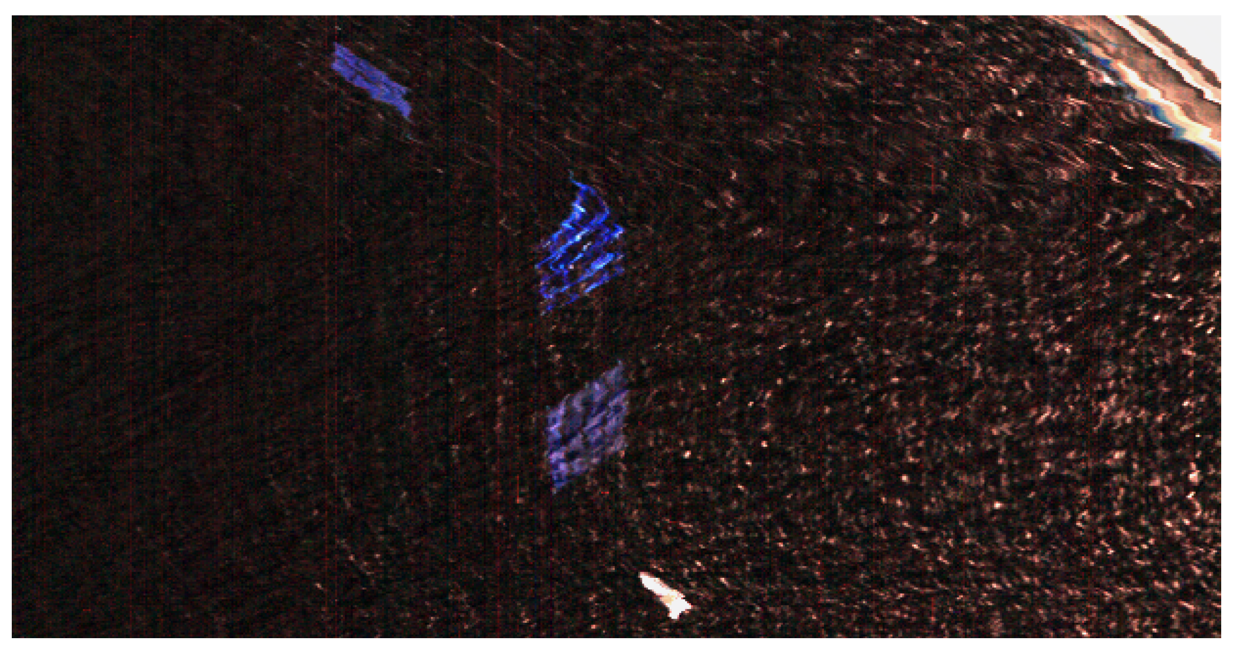
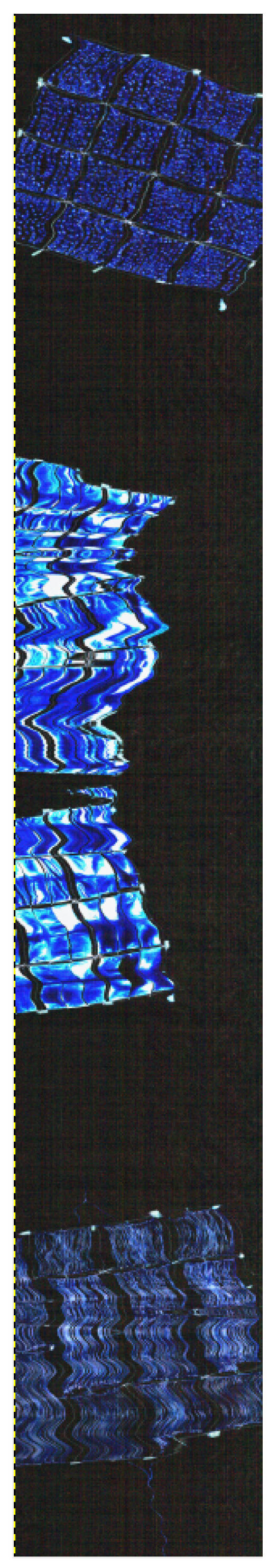
In Figure A1 it is possible to observe the waterfall image from the flight, with 500–600 m altitude.
Figure A1.
Waterfall image of the flyby analyzed from the 18/9 afternoon F-BUMA flight.

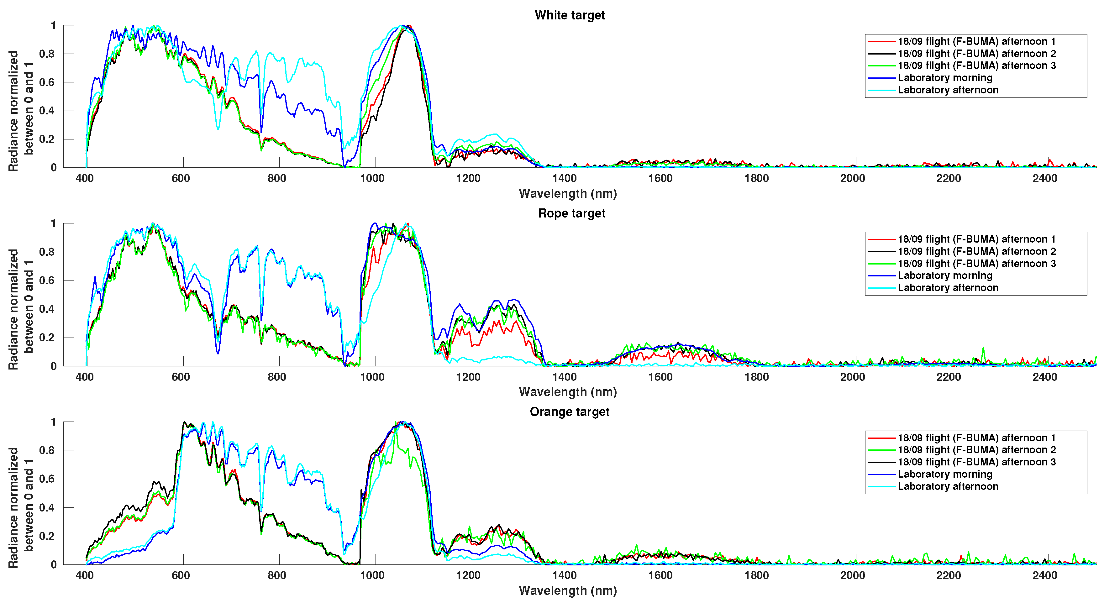
In Figure A2 is possible to see the spectral response (in normalized radiance) for all the three targets, compared with laboratory results for the wet samples.
Figure A2.
Results for the 18/9 F-BUMA afternoon flight, analyzing 3 different pixels (bright pixel-afternoon 1, a medium pixel-afternoon 2 and a dark pixel-afternoon 3) for each material, and comparing them to the laboratory results.
Figure A2.
Results for the 18/9 F-BUMA afternoon flight, analyzing 3 different pixels (bright pixel-afternoon 1, a medium pixel-afternoon 2 and a dark pixel-afternoon 3) for each material, and comparing them to the laboratory results.

Appendix A.2. Grifo-X Flight Data
In Figure A3 is possible to see the results for this flight, with 25–35 m altitude.
Figure A3.
Waterfall image of the flyby analyzed from the 25/9 Grifo-X flight 1.

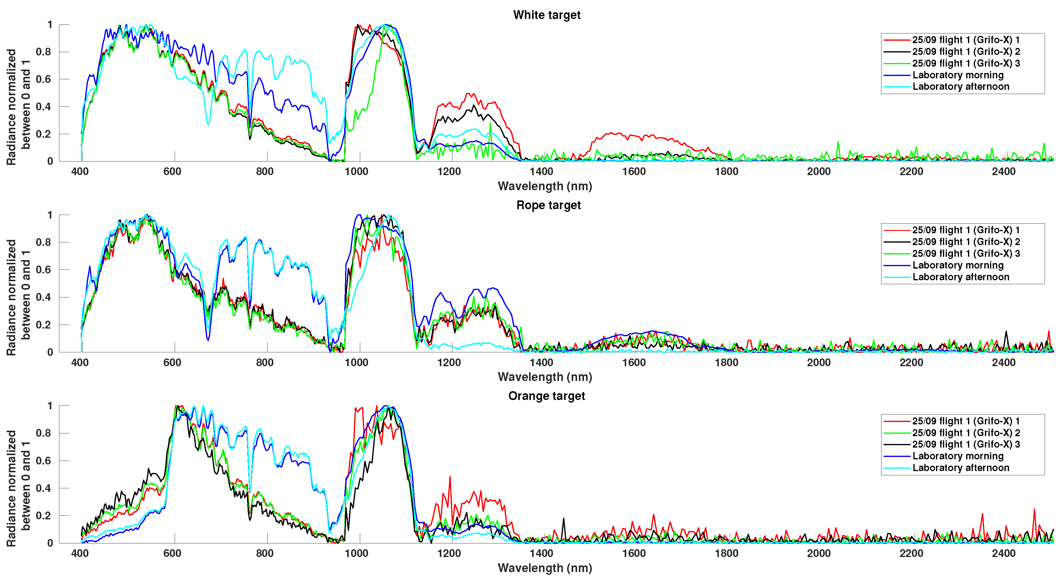
In Figure A4 is possible to see the obtained results for all the targets.
Figure A4.
Results for the 25/9 Grifo-X first flight, analyzing 3 different pixels (bright pixel-1, a medium pixel-2 and a dark pixel -3) for each material, and comparing them to the laboratory results.
Figure A4.
Results for the 25/9 Grifo-X first flight, analyzing 3 different pixels (bright pixel-1, a medium pixel-2 and a dark pixel -3) for each material, and comparing them to the laboratory results.

Figure A5 shows a comparison between the bright pixels for the 25/09 flight 1 with Grifo-X, 20/09 F-BUMA flight and the laboratory morning results for all the target materials.
Figure A5.
Comparison between the bright pixels for the 25/09 flight 1 with Grifo-X, 20/09 F-BUMA flight and the laboratory morning results for all the target materials.
Figure A5.
Comparison between the bright pixels for the 25/09 flight 1 with Grifo-X, 20/09 F-BUMA flight and the laboratory morning results for all the target materials.

Figure A6 shows a comparison between the data from the same target (rope) at three different situations: F-BUMA flight at 600 m altitude, Grifo-X flight at 20 m altitude and using the laboratory setup.
Figure A6.
Comparison between the rope target results for F-BUMA flight (600 m altitude), Grifo-X flight (20 m altitude) and laboratory setup, with focus in HySpex Mjolnir S-620 bands (970–2500 nm).
Figure A6.
Comparison between the rope target results for F-BUMA flight (600 m altitude), Grifo-X flight (20 m altitude) and laboratory setup, with focus in HySpex Mjolnir S-620 bands (970–2500 nm).

References
- Ruiz, I.; Basurko, O.C.; Rubio, A.; Delpey, M.; Granado, I.; Declerck, A.; Mader, J.; Cózar, A. Litter Windrows in the South-East Coast of the Bay of Biscay: An Ocean Process Enabling Effective Active Fishing for Litter. Front. Mar. Sci. 2020, 7, 308. [Google Scholar] [CrossRef]
- Ryan, P.G. A Brief History of Marine Litter Research. In Marine Anthropogenic Litter; Bergmann, M., Gutow, L., Klages, M., Eds.; Springer International Publishing: Cham, Switzerland, 2015; pp. 1–25. [Google Scholar] [CrossRef] [Green Version]
- Lebreton, L.; Slat, B.; Ferrari, F.; Sainte-Rose, B.; Aitken, J.; Marthouse, R.; Hajbane, S.; Cunsolo, S.; Schwarz, A.; Levivier, A.; et al. Evidence that the Great Pacific Garbage Patch is rapidly accumulating plastic. Sci. Rep. 2018, 8, 4666. [Google Scholar] [CrossRef] [PubMed] [Green Version]
- McIlgorm, A.; Campbell, H.F.; Rule, M.J. The economic cost and control of marine debris damage in the Asia-Pacific region. Ocean. Coast. Manag. 2011, 54, 643–651. [Google Scholar] [CrossRef]
- Barboza, L.G.A.; Dick Vethaak, A.; Lavorante, B.R.; Lundebye, A.K.; Guilhermino, L. Marine microplastic debris: An emerging issue for food security, food safety and human health. Mar. Pollut. Bull. 2018, 133, 336–348. [Google Scholar] [CrossRef]
- Rodríguez, Y.; Ressurreição, A.; Pham, C.K. Socio-economic impacts of marine litter for remote oceanic islands: The case of the Azores. Mar. Pollut. Bull. 2020, 160, 111631. [Google Scholar] [CrossRef]
- Pieper, C.; Magalhães Loureiro, C.; Law, K.; Amaral-Zettler, L.; Quintino, V.; Rodrigues, A.; Ventura, M.; Martins, A. Marine litter footprint in the Azores Islands: A climatological perspective. Sci. Total Environ. 2021, 761, 143310. [Google Scholar] [CrossRef] [PubMed]
- Veiga, J.; Fleet, D.; Kinsey, S.; Nilsson, P.; Vlachogianni, T.; Werner, S.; Galgani, F.; Thompson, R.; Dagevos, J.; Gago, J.; et al. Identifying Sources of Marine Litter. JRC Technical Report; Publications Office of the European Union: Luxembourg, 2016; p. 41. [Google Scholar] [CrossRef]
- Lee, J.; Lee, J.S.; Jang, Y.C.; Hong, S.Y.; Shim, W.J.; Song, Y.K.; Hong, S.H.; Jang, M.; Han, G.M.; Kang, D.; et al. Distribution and Size Relationships of Plastic Marine Debris on Beaches in South Korea. Arch. Environ. Contam. Toxicol. 2015, 69, 288–298. [Google Scholar] [CrossRef]
- Ryan, P.G.; Moore, C.J.; Van Franeker., A.J.; Moloney, C.L. Monitoring the abundance of plastic debris in the marine environment. Philos. Trans. R. Soc. Biol. Sci. 2009, 364, 1999–2012. [Google Scholar] [CrossRef] [Green Version]
- Goddijn-Murphy, L.; Peters, S.; Van Sebille, E.; James, N.A.; Gibb, S. Concept for a hyperspectral remote sensing algorithm for floating marine macro plastics. Mar. Pollut. Bull. 2018, 126, 255–262. [Google Scholar] [CrossRef] [Green Version]
- Ryan, P.G. Does size and buoyancy affect the long-distance transport of floating debris? Environ. Res. Lett. 2015, 10, 084019. [Google Scholar] [CrossRef]
- Van Sebille, E.; Wilcox, C.; Lebreton, L.; Maximenko, N.; Hardesty, B.D.; Van Franeker, J.A.; Eriksen, M.; Siegel, D.; Galgani, F.; Law, K.L. A global inventory of small floating plastic debris. Environ. Res. Lett. 2015, 10. [Google Scholar] [CrossRef]
- Derraik, J.G.B. The pollution of the marine environment by plastic debris: A review. Mar. Pollut. Bull. 2002, 44, 842–852. [Google Scholar] [CrossRef]
- Garrity, S.D.; Levings, S.C. Marine debris along the Caribbean coast of Panama. Mar. Pollut. Bull. 1993, 26, 317–324. [Google Scholar] [CrossRef]
- Willoughby, N.G.; Sangkoyo, H.; Lakaseru, B.O. Beach litter: An increasing and changing problem for Indonesia. Mar. Pollut. Bull. 1997, 34, 469–478. [Google Scholar] [CrossRef]
- Clark, R.B.; Frid, C.; Attrill, M. Marine Pollution; Clarendon Press: Oxford, UK, 1989; Volume 4. [Google Scholar]
- Islam, M.S.; Tanaka, M. Impacts of pollution on coastal and marine ecosystems including coastal and marine fisheries and approach for management: A review and synthesis. Mar. Pollut. Bull. 2004, 48, 624–649. [Google Scholar] [CrossRef] [PubMed]
- Zielinski, O.; Busch, J.A.; Cembella, A.D.; Daly, K.L.; Engelbrektsson, J.; Hannides, A.K.; Schmidt, H. Detecting marine hazardous substances and organisms: Sensors for pollutants, toxins, and pathogens. Ocean. Sci. 2009, 5, 329–349. [Google Scholar] [CrossRef] [Green Version]
- Brekke, C.; Solberg, A.H. Oil spill detection by satellite remote sensing. Remote Sens. Environ. 2005, 95, 1–13. [Google Scholar] [CrossRef]
- Zielinski, O.; Hengstermann, T.; Robbe, N. Detection of oil spills by airborne sensors. Mar. Surf. Film. 2006, 255–271. [Google Scholar] [CrossRef]
- Dekker, A.G.; Brando, V.E.; Anstee, J.M.; Pinnel, N.; Kutser, T.; Hoogenboom, E.J.; Peters, S.; Pasterkamp, R.; Vos, R.; Olbert, C.; et al. Imaging spectrometry of water. Imaging Spectrom. 2002, 4, 307–359. [Google Scholar]
- Topouzelis, K.; Papakonstantinou, A.; Singha, S.; Li, X.; Poursanidis, D. Editorial on Special Issue “Applications of Remote Sensing in Coastal Areas”. Remote Sens. 2020, 12, 974. [Google Scholar] [CrossRef] [Green Version]
- Papakonstantinou, A.; Batsaris, M.; Spondylidis, S.; Topouzelis, K. A Citizen Science Unmanned Aerial System Data Acquisition Protocol and Deep Learning Techniques for the Automatic Detection and Mapping of Marine Litter Concentrations in the Coastal Zone. Drones 2021, 5, 6. [Google Scholar] [CrossRef]
- Wolf, M.; van den Berg, K.; Garaba, S.P.; Gnann, N.; Sattler, K.; Stahl, F.; Zielinski, O. Machine learning for aquatic plastic litter detection, classification and quantification (APLASTIC-Q). Environ. Res. Lett. 2020, 15, 114042. [Google Scholar] [CrossRef]
- Gonçalves, G.; Andriolo, U.; Pinto, L.; Bessa, F. Mapping marine litter using UAS on a beach-dune system: A multidisciplinary approach. Sci. Total Environ. 2020, 706, 135742. [Google Scholar] [CrossRef]
- Gonçalves, G.; Andriolo, U.; Pinto, L.; Duarte, D. Mapping marine litter with Unmanned Aerial Systems: A showcase comparison among manual image screening and machine learning techniques. Mar. Pollut. Bull. 2020, 155, 111158. [Google Scholar] [CrossRef] [PubMed]
- Garaba, S.P.; Dierssen, H.M. An airborne remote sensing case study of synthetic hydrocarbon detection using short wave infrared absorption features identified from marine-harvested macro- and microplastics. Remote Sens. Environ. 2018, 205, 224–235. [Google Scholar] [CrossRef]
- Acuña-Ruz, T.; Uribe, D.; Taylor, R.; Amézquita, L.; Guzmán, M.C.; Merrill, J.; Martínez, P.; Voisin, L.; Mattar, B.C. Anthropogenic marine debris over beaches: Spectral characterization for remote sensing applications. Remote Sens. Environ. 2018, 217, 309–322. [Google Scholar] [CrossRef]
- Topouzelis, K.; Papakonstantinou, A.; Garaba, S.P. Detection of floating plastics from satellite and unmanned aerial systems (Plastic Litter Project 2018). Int. J. Appl. Earth Obs. Geoinf. 2019, 79, 175–183. [Google Scholar] [CrossRef]
- Agency, E.S.; PML. Remote Sensing of Marine Litter OPTIMAL-Optical Methods for Marine Litter Detection Final Report (D7); Plymouth Marine Laboratory (PML): Plymouth, UK, 2020. [Google Scholar]
- Biermann, L.; Clewley, D.; Martinez-Vicente, V.; Topouzelis, K. Finding Plastic Patches in Coastal Waters using Optical Satellite Data. Sci. Rep. 2020, 10, 5364. [Google Scholar] [CrossRef] [Green Version]
- Kremezi, M.; Kristollari, V.; Karathanassi, V.; Topouzelis, K.; Kolokoussis, P.; Taggio, N.; Aiello, A.; Ceriola, G.; Barbone, E.; Corradi, P. Pansharpening PRISMA Data for Marine Plastic Litter Detection Using Plastic Indexes. IEEE Access 2021, 9, 61955–61971. [Google Scholar] [CrossRef]
- Freitas, S.; Silva, H.; Almeida, J.; Silva, E. Hyperspectral Imaging for Real-Time Unmanned Aerial Vehicle Maritime Target Detection. J. Intell. Robot. Syst. 2018, 90, 551–570. [Google Scholar] [CrossRef] [Green Version]
- Arroyo-Mora, J.P.; Kalacska, M.; Løke, T.; Schläpfer, D.; Coops, N.C.; Lucanus, O.; Leblanc, G. Assessing the impact of illumination on UAV pushbroom hyperspectral imagery collected under various cloud cover conditions. Remote Sens. Environ. 2021, 258, 112396. [Google Scholar] [CrossRef]
- Breiman, L. Random Forests. Mach. Learn. 2001, 45, 5–32. [Google Scholar] [CrossRef] [Green Version]
- Boser, B.; Guyon, I.; Vapnik, V. A training algorithm for optimal margin classifiers. In Proceedings of the Fifth Annual Workshop on Computational Learning Theory, Pittsburgh, PA, USA, 27–29 July 1992. [Google Scholar]
Figure 1.
Porto Pim Bay Faial Island Azores.

Figure 2.
Marine Litter found in the test site, Porto Pim Bay (Faial Island, Azores).

Figure 3.
Connections between the hyperspectral cameras, data acquisition computers and GPS/INS.

Figure 4.
Test setup used during the laboratory test.

Figure 5.
Hyperspectral imaging system mounted in the manned aircraft (F-BUMA).

Figure 6.
Hyperspectral imaging system mounted in the unmanned aircraft (Grifo-X).

Figure 7.
Plastics used in the targets and the laboratory results in normalized radiance for each target material: (a) shows the orange target material (with approximately 20 cm diameter), (b,c) shows the laboratory results for the orange target material, respectively; (d) shows the white target material (with approximately 50 cm width, with variable length), (e,f) shows the laboratory results for the orange target material, respectively; (g) shows the thin rope target material (3 cm diameter, with variable length), (h,i) shows the laboratory results for the orange target material, respectively; (j) shows the thick rope target material (5 cm diameter, with variable length), (k,l) shows the laboratory results for the orange target material, respectively.

Figure 8.
Picture of the three targets used. From left to the right: low density polyethylene orange target (with used oyster spat collectors), white plastic film target and rope target.
Figure 8.
Picture of the three targets used. From left to the right: low density polyethylene orange target (with used oyster spat collectors), white plastic film target and rope target.

Figure 9.
Flight trajectories: (a) shows the 20 September 2020 flight trajectory, performed by F-BUMA aircraft, while in (b) is possible to observe the trajectory of the 25 September 2020 flight performed with GRIFO-X aircraft.
Figure 9.
Flight trajectories: (a) shows the 20 September 2020 flight trajectory, performed by F-BUMA aircraft, while in (b) is possible to observe the trajectory of the 25 September 2020 flight performed with GRIFO-X aircraft.

Table 2.
Specim FX10e and HySpex Mjolnir S-620 main characteristics.
| Specifications | Specim FX10e | HySpex Mjolnir S-620 |
|---|---|---|
| Spectral range | 400–1000 nm | 970–2500 nm |
| Spatial pixels | 1024 | 620 |
| Spectral channels and sampling | 224 bands @ 2.7 nm | 300 bands @ 5.1 nm |
| F-number | F1.7 | F1.9 |
| FOV | 38° | 20° |
| Max speed | 330 fps | 100 fps |
| Power consumption | 4W (12DC) | 70 W (9–32 V) |
| Dimensions (l × w × h) | 150 mm × 85 mm × 71 mm | 374 mm × 202 mm × 178 mm |
| Weight | 1.3 kg | 6 kg (including IMU/GPS and DAU) 6.5 kg (including also standard battery) |
Table 3.
Targets used during the dataset collection and their division between the classes.
| Class 0 Water and Land (Houses, Trees, Streets, Cars, and Others Materials) | Class 1 Orange Plastic Target | Class 2 White Plastic Target | Class 3 Ropes Target |
|---|---|---|---|
 |  |  |  |
Table 4.
Number of pixels (NP) present for each class in 18/9 F-BUMA flight: class 1 corresponds to the orange target data, class 2 to the white target and class 3 to the rope target data. Class 0 was created with all the remaining pixels, containing both land and water data.
Table 4.
Number of pixels (NP) present for each class in 18/9 F-BUMA flight: class 1 corresponds to the orange target data, class 2 to the white target and class 3 to the rope target data. Class 0 was created with all the remaining pixels, containing both land and water data.
| Flyby | Class 0 (NP) | Class 1 (NP) | Class 2 (NP) | Class 3 (NP) |
|---|---|---|---|---|
| 0 | 57,259 | 299 | 664 | 678 |
| 1 | 125,732 | 399 | 857 | 732 |
| 2 | 86,479 | 454 | 1203 | 1144 |
| 3 | 153,180 | 462 | 1880 | 1338 |
| 4 | 51,438 | 700 | 1182 | 0 |
| 5 | 138,612 | 620 | 1658 | 1710 |
| 6 | 87,266 | 696 | 1358 | 1200 |
| 7 | 117,078 | 489 | 1373 | 1960 |
Table 5.
Number of pixels (NP) present for each class in 20/9 F-BUMA flight: class 1 corresponds to the orange target data, class 2 to the white target and class 3 to the rope target data. Class 0 was created with all the remaining pixels, containing both land and water data.
Table 5.
Number of pixels (NP) present for each class in 20/9 F-BUMA flight: class 1 corresponds to the orange target data, class 2 to the white target and class 3 to the rope target data. Class 0 was created with all the remaining pixels, containing both land and water data.
| Flyby | Class 0 (NP) | Class 1 (NP) | Class 2 (NP) | Class 3 (NP) |
|---|---|---|---|---|
| 0 | 15,604 | 516 | 0 | 0 |
| 1 | 29,522 | 858 | 0 | 0 |
| 2 | 47,986 | 662 | 671 | 281 |
| 3 | 72,742 | 715 | 1157 | 1026 |
| 4 | 52,024 | 626 | 670 | 0 |
| 5 | 94,414 | 1246 | 781 | 899 |
| 6 | 167,177 | 1547 | 1682 | 2574 |
| 7 | 81,713 | 813 | 864 | 930 |
| 8 | 183,419 | 2640 | 1928 | 1733 |
Table 6.
Results obtained for the test data (20/09/2020 flight) for random forest (RF) and support vector machine (SVM) algorithms.
Table 6.
Results obtained for the test data (20/09/2020 flight) for random forest (RF) and support vector machine (SVM) algorithms.
| Flyby 2 | ||||||||
|---|---|---|---|---|---|---|---|---|
| RF | SVM | |||||||
| Class | Precision | Recall | F1-Score | Accuracy | Precision | Recall | F1-Score | Accuracy |
| 0 | 0.99 | 1 | 0.99 | 97.35 % | 0.99 | 0.99 | 0.99 | 97.47 % |
| 1 | 0.24 | 0.12 | 0.16 | 0.75 | 0.42 | 0.54 | ||
| 2 | 0.85 | 0.42 | 0.56 | 0.66 | 0.47 | 0.55 | ||
| 3 | 0.18 | 0.44 | 0.26 | 0.22 | 0.50 | 0.31 | ||
| Flyby 3 | ||||||||
| RF | SVM | |||||||
| Class | Precision | Recall | F1-Score | Accuracy | Precision | Recall | F1-Score | Accuracy |
| 0 | 0.99 | 1 | 0.99 | 97.34 % | 0.99 | 0.99 | 0.99 | 97.27 % |
| 1 | 0.20 | 0.13 | 0.16 | 0.75 | 0.38 | 0.51 | ||
| 2 | 0.85 | 0.53 | 0.65 | 0.56 | 0.43 | 0.49 | ||
| 3 | 0.45 | 0.38 | 0.41 | 0.52 | 0.74 | 0.61 | ||
| RF | SVM | |||||||
| Class | Precision | Recall | F1-Score | Accuracy | Precision | Recall | F1-Score | Accuracy |
| 0 | 0.99 | 1 | 0.99 | 98.09 % | 0.99 | 0.99 | 0.99 | 97.06 % |
| 1 | 0.71 | 0.25 | 0.37 | 0.77 | 0.46 | 0.58 | ||
| 2 | 0.74 | 0.62 | 0.67 | 0.57 | 0.59 | 0.58 | ||
| 3 | 0.38 | 0.56 | 0.45 | 0.21 | 0.47 | 0.29 | ||
| Flyby 6 | ||||||||
| RF | SVM | |||||||
| Class | Precision | Recall | F1-Score | Accuracy | Precision | Recall | F1-Score | Accuracy |
| 0 | 0.99 | 1 | 0.99 | 97.92 % | 0.99 | 0.98 | 0.98 | 96.56 % |
| 1 | 0.52 | 0.22 | 0.31 | 0.71 | 0.48 | 0.57 | ||
| 2 | 0.85 | 0.59 | 0.70 | 0.78 | 0.67 | 0.72 | ||
| 3 | 0.50 | 0.42 | 0.46 | 0.27 | 0.51 | 0.35 | ||
| Flyby 7 | ||||||||
| RF | SVM | |||||||
| Class | Precision | Recall | F1-Score | Accuracy | Precision | Recall | F1-Score | Accuracy |
| 0 | 0.98 | 1 | 0.99 | 97.32 % | 1 | 0.99 | 0.99 | 98.01 % |
| 1 | 0.01 | 0 | 0.01 | 0.50 | 0.16 | 0.24 | ||
| 2 | 0.95 | 0.45 | 0.61 | 0.44 | 0.72 | 0.54 | ||
| 3 | 0.17 | 0.01 | 0.02 | 0.64 | 0.76 | 0.70 | ||
| Flyby 8 | ||||||||
| RF | SVM | |||||||
| Class | Precision | Recall | F1-Score | Accuracy | Precision | Recall | F1-Score | Accuracy |
| 0 | 0.99 | 0.99 | 0.99 | 97.44 % | 0.99 | 0.99 | 0.99 | 97.28 % |
| 1 | 0.85 | 0.55 | 0.66 | 0.10 | 0.02 | 0.04 | ||
| 2 | 0.94 | 0.36 | 0.52 | 0.46 | 0.55 | 0.50 | ||
| 3 | 0.21 | 0.35 | 0.26 | 0.30 | 0.51 | 0.38 | ||
Table 7.
Figures showing the results obtained for the test data (20 September 2020 flight) for random forest (RF) and support vector machine (SVM) algorithms. In the first column are illustrated the ground-truth for each flyby, the second column shows the prediction made by the random forest algorithm, and the last column represents the predicted values by the support vector machine algorithm.
| Flyby 2 | ||
|---|---|---|
 |  |  |
| Flyby 3 | ||
 |  |  |
| Flyby 5 | ||
 |  |  |
| Flyby 6 | ||
 |  |  |
| Flyby 7 | ||
 |  |  |
| Flyby 8 | ||
 |  |  |
Publisher’s Note: MDPI stays neutral with regard to jurisdictional claims in published maps and institutional affiliations. |
© 2021 by the authors. Licensee MDPI, Basel, Switzerland. This article is an open access article distributed under the terms and conditions of the Creative Commons Attribution (CC BY) license (https://creativecommons.org/licenses/by/4.0/).
Share and Cite
MDPI and ACS Style
Freitas, S.; Silva, H.; Silva, E. Remote Hyperspectral Imaging Acquisition and Characterization for Marine Litter Detection. Remote Sens. 2021, 13, 2536. https://0-doi-org.brum.beds.ac.uk/10.3390/rs13132536
AMA Style
Freitas S, Silva H, Silva E. Remote Hyperspectral Imaging Acquisition and Characterization for Marine Litter Detection. Remote Sensing. 2021; 13(13):2536. https://0-doi-org.brum.beds.ac.uk/10.3390/rs13132536
Chicago/Turabian StyleFreitas, Sara, Hugo Silva, and Eduardo Silva. 2021. "Remote Hyperspectral Imaging Acquisition and Characterization for Marine Litter Detection" Remote Sensing 13, no. 13: 2536. https://0-doi-org.brum.beds.ac.uk/10.3390/rs13132536
Note that from the first issue of 2016, this journal uses article numbers instead of page numbers. See further details here.