
Modified Linear Scaling and Quantile Mapping Mean Bias Correction of MODIS Land Surface Temperature for Surface Air Temperature Estimation for the Lowland Areas of Peninsular Malaysia

 , ,
, ,
Abstract
:1. Introduction
2. Materials and Methods
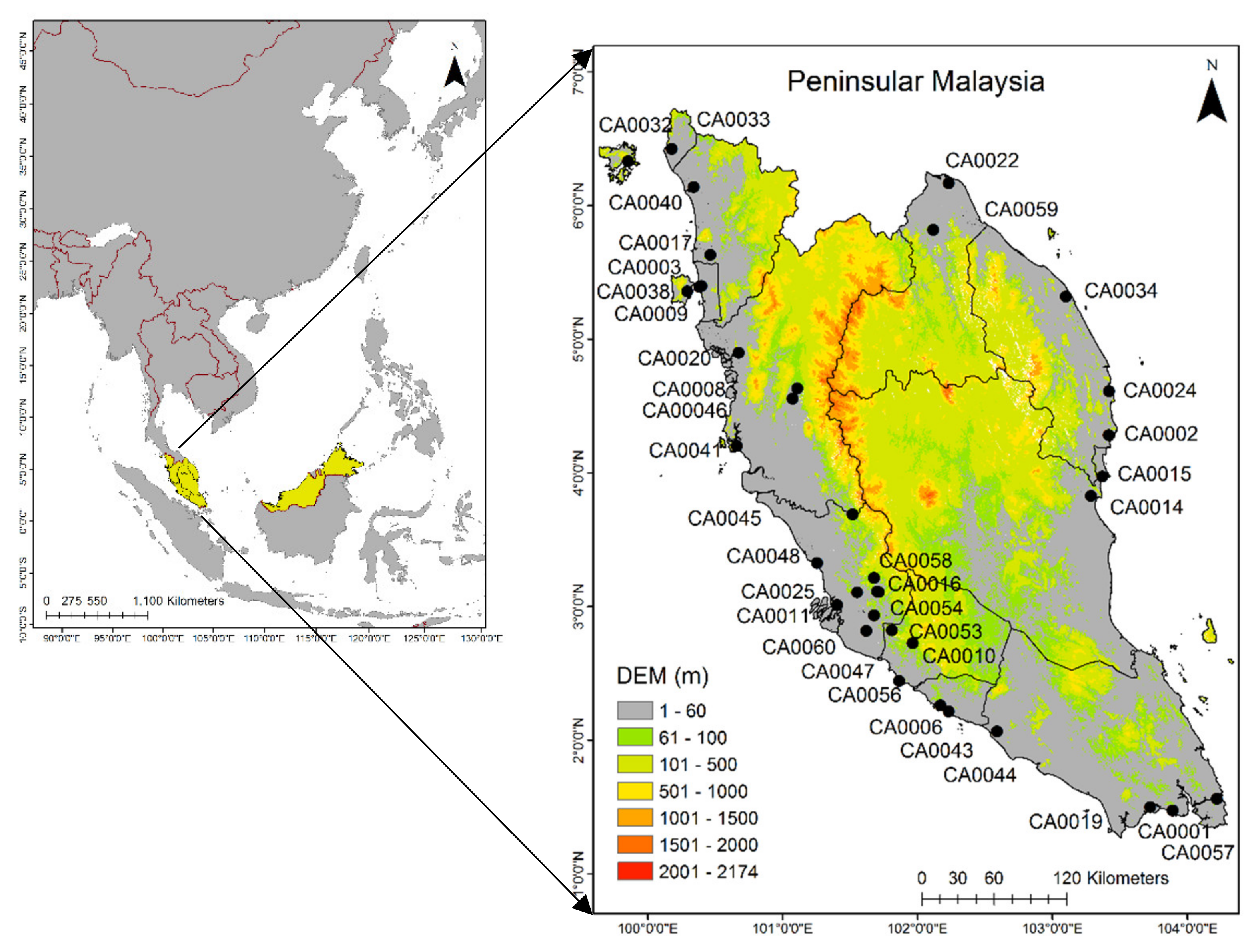
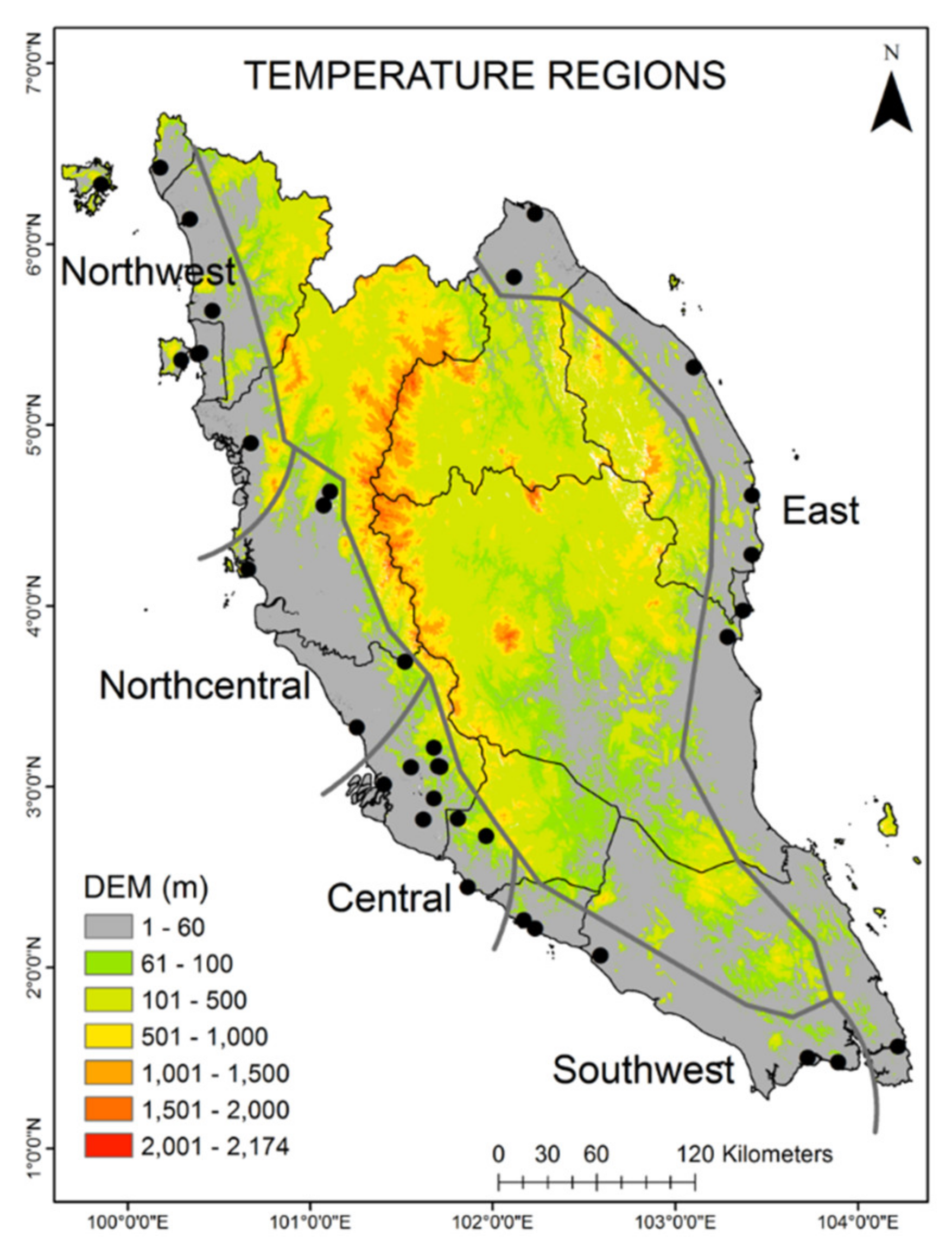
2.1. Study Area
2.2. Data Collection
2.2.1. Ground Measurement
2.2.2. MODIS LST Product
2.3. Data Processing
2.3.1. Pre-Processing of Ta
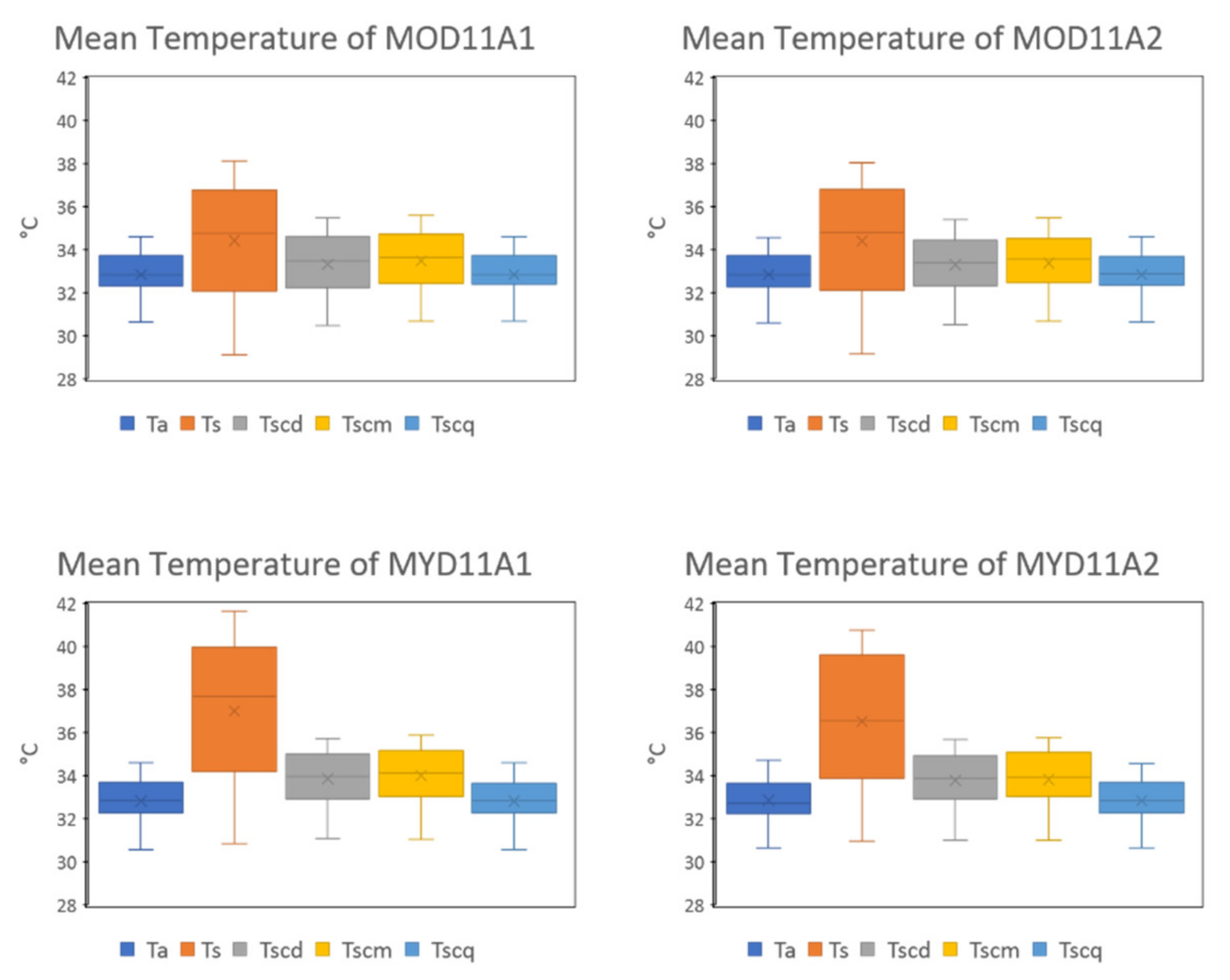
2.3.2. Pre-Processing of Ts
2.4. Region Delineation
Preparing Regional Data
2.5. Data Analysis
2.5.1. Evaluation Metrics
2.5.2. Mean Bias Correction (MBC)
3. Results
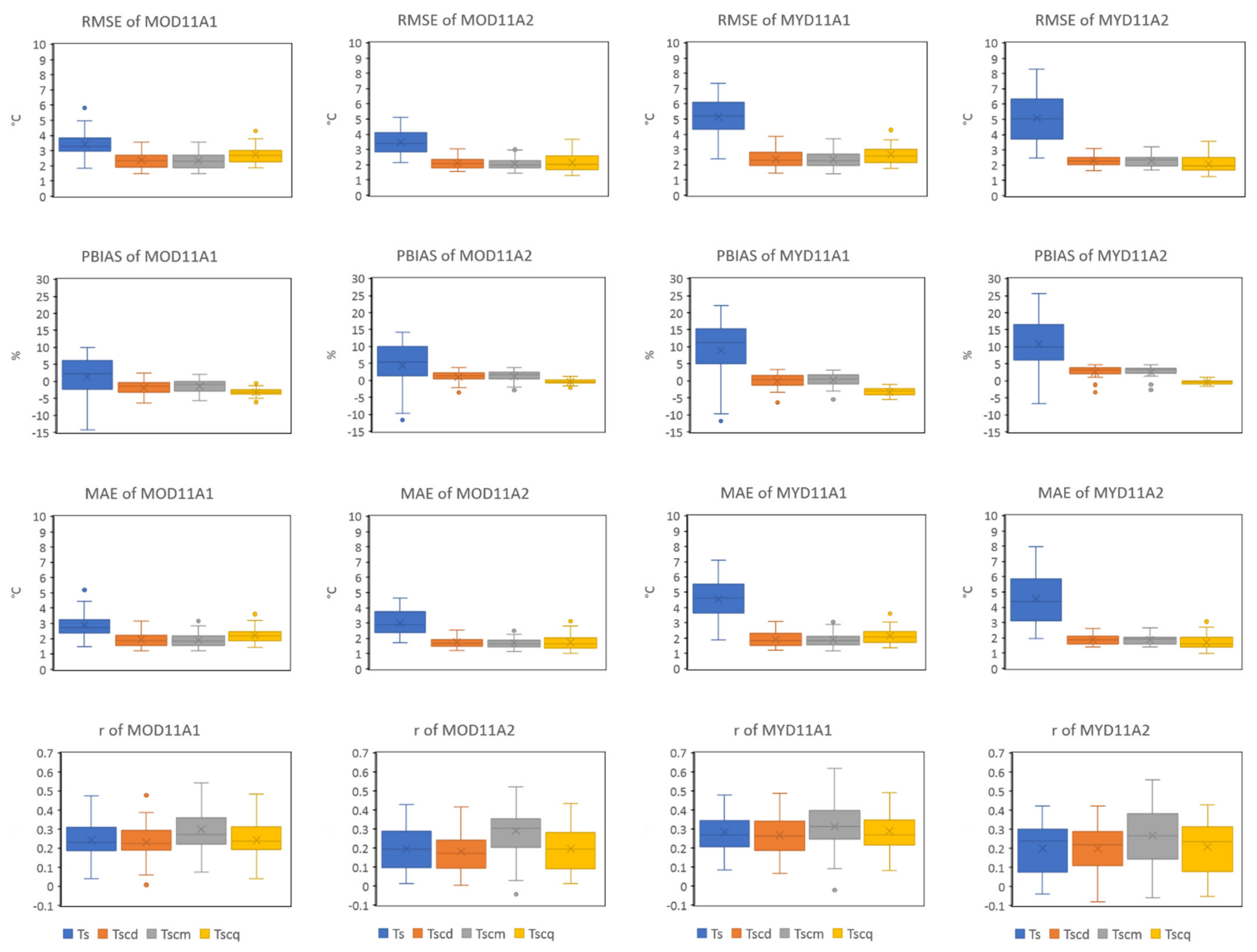
3.1. Evaluation Metrics for Pre- and Post-MBC against Ta by Station
3.1.1. RMSE
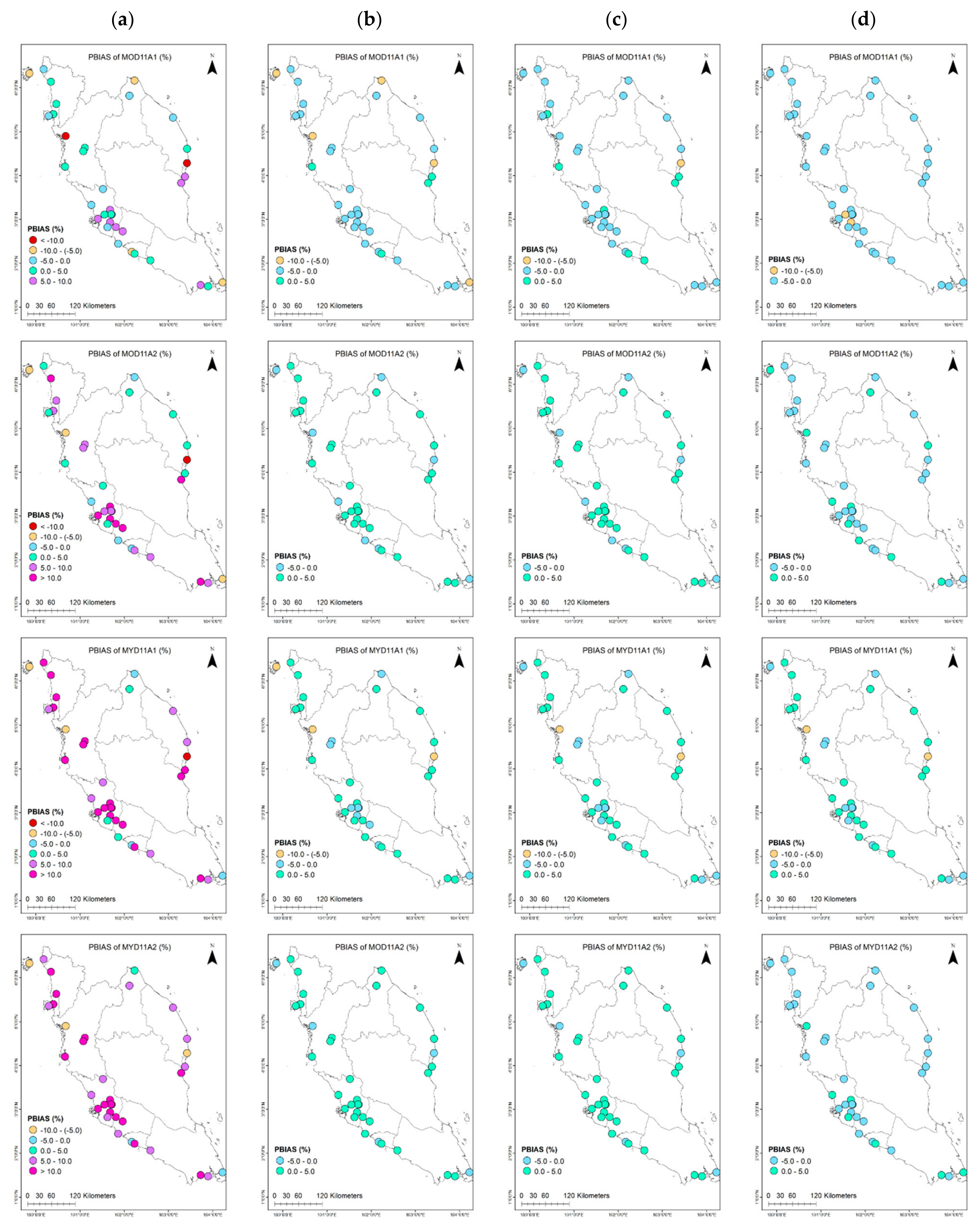
3.1.2. PBIAS
3.1.3. MAE
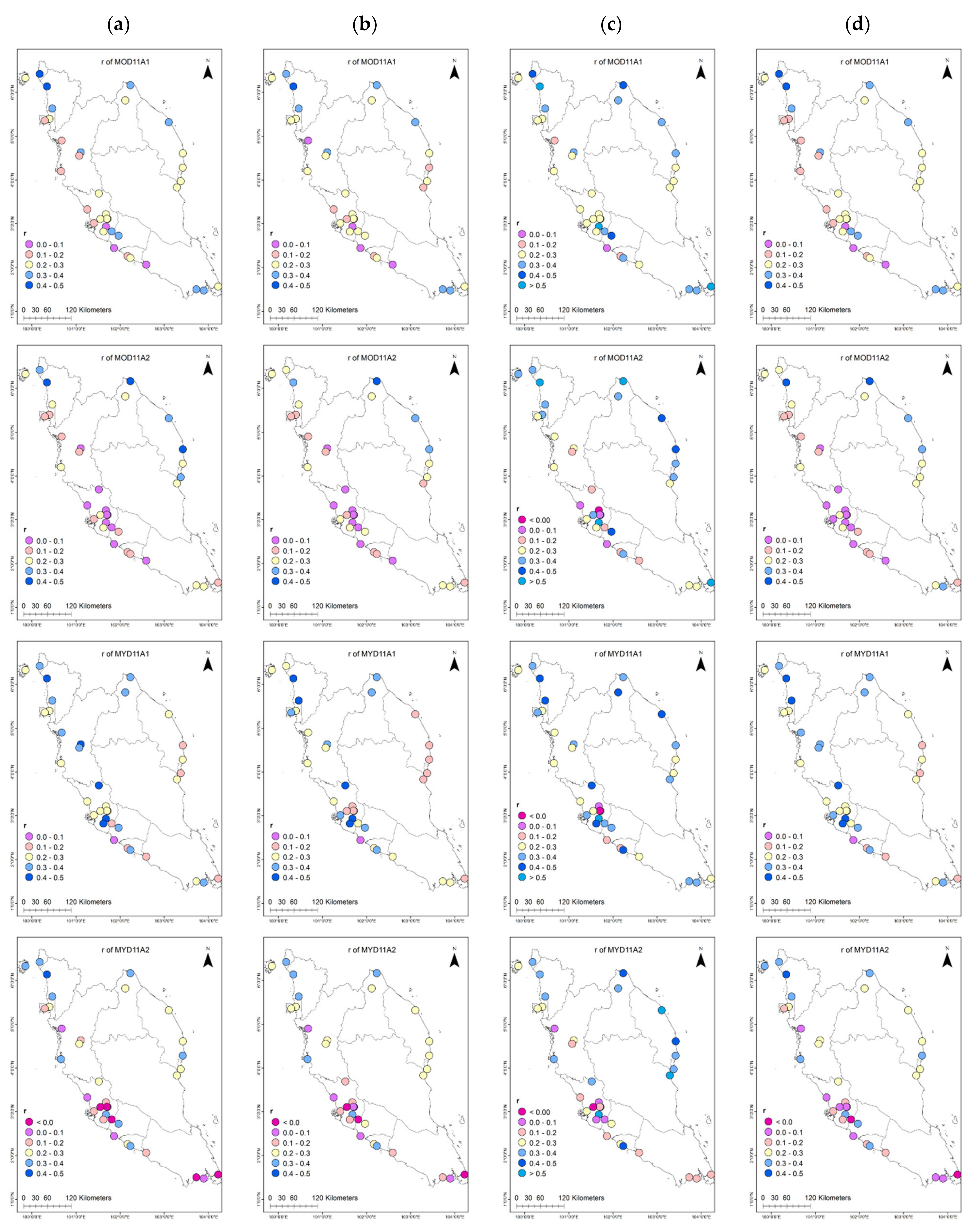
3.1.4. Correlation Coefficient (r)
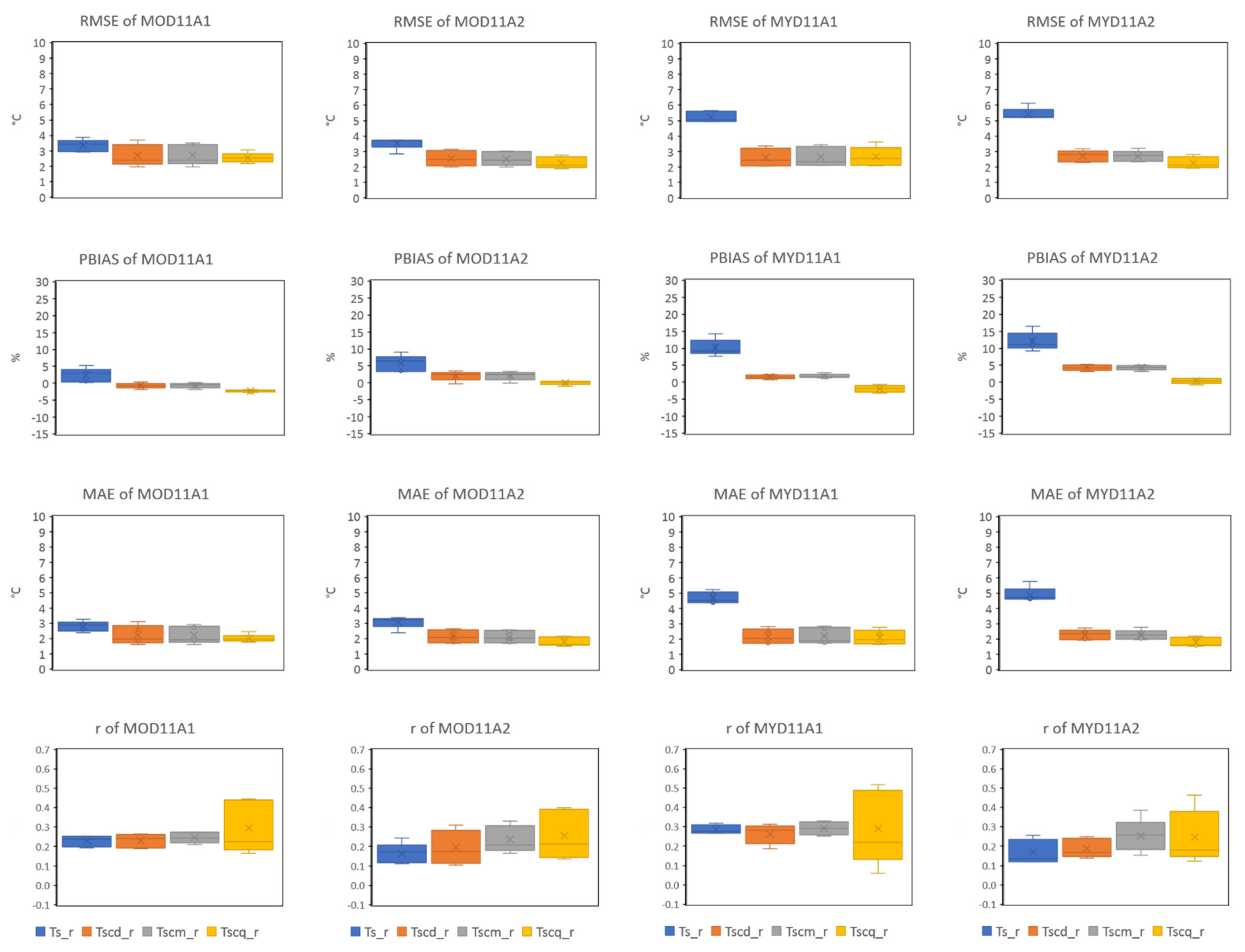
3.2. Evaluation Metrics for Pre- and Post-MBC against Ta by Region
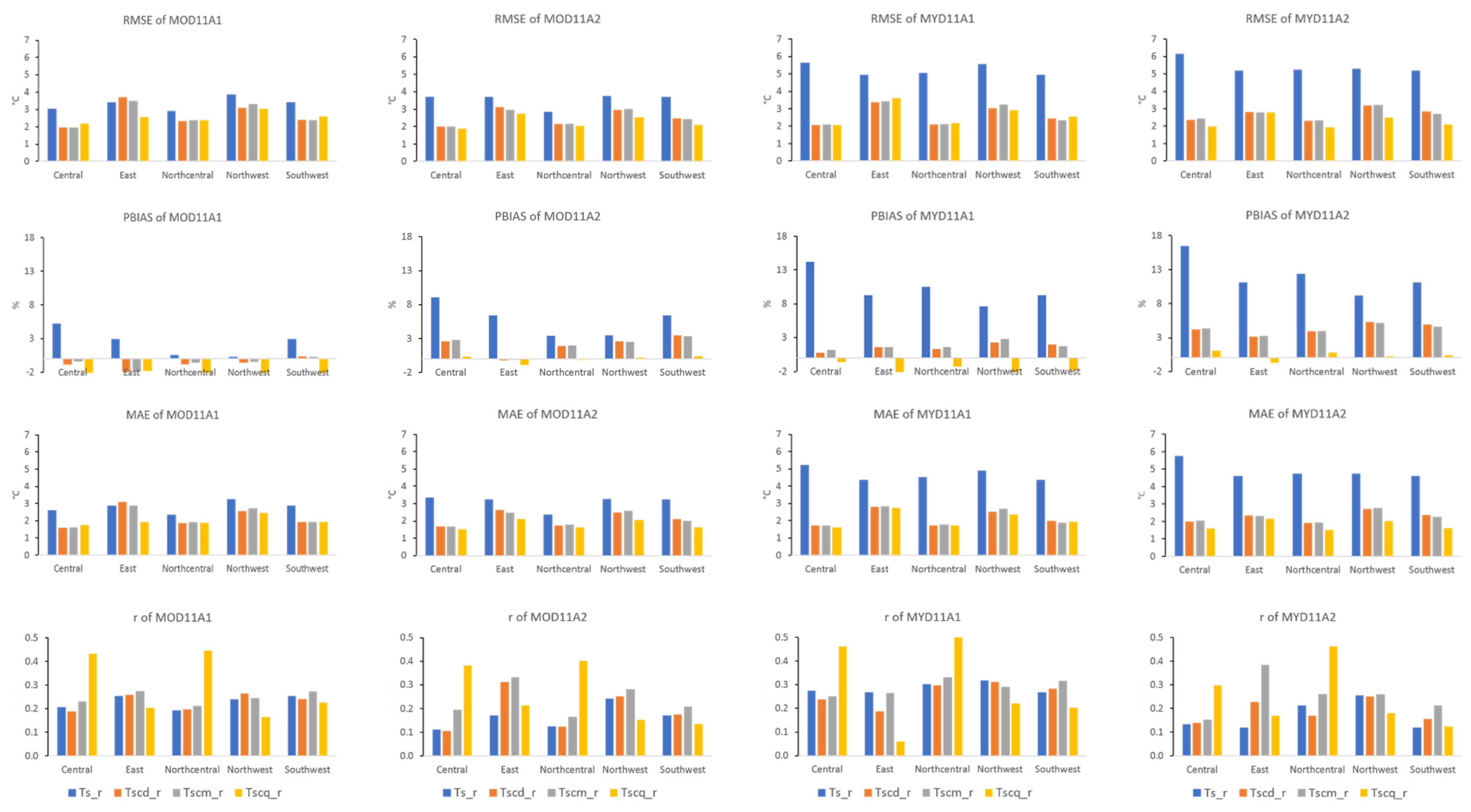
3.2.1. RMSE
3.2.2. PBIAS
3.2.3. MAE
3.2.4. Correlation Coefficient (r)
4. Discussion
4.1. By Station Performance
4.2. By Region Performance
4.3. Limitations and Future Works
5. Conclusions
Author Contributions
Funding
Data Availability Statement
Acknowledgments
Conflicts of Interest
References
- Tangang, F.T.; Juneng, L.; Ahmad, S. Trend and interannual variability of temperature in Malaysia: 1961–2002. Theor. Appl. Climatol. 2007, 89, 127–141. [Google Scholar] [CrossRef]
- Wai, N.M.; Camerlengo, A.; Khairi, A.; Wahab, A. A Study of Global Warming in Malaysia. J. Teknol. 2005, 42, 1–10. [Google Scholar]
- Abraha, M.G.; Savage, M.J. Comparison of estimates of daily solar radiation from air temperature range for application in crop simulations. Agric. For. Meteorol. 2008, 148, 401–416. [Google Scholar] [CrossRef]
- Svensson, M.K.; Eliasson, I. Diurnal air temperatures in built-up areas in relation to urban planning. Landsc. Urban Plan. 2002, 61, 37–54. [Google Scholar] [CrossRef]
- Wu, T.; Li, Y. Spatial interpolation of temperature in the United States using residual kriging. Appl. Geogr. 2013, 44, 112–120. [Google Scholar] [CrossRef]
- Jin, M.; Dickinson, R.E. Land surface skin temperature climatology: Benefitting from the strengths of satellite observations. Environ. Res. Lett. 2010, 5, 044004. [Google Scholar] [CrossRef] [Green Version]
- Jin, M.; Dickinson, R.E.; Vogelmann, A.M. A comparison of CCM2-BATS skin temperature and surface-air temperature with satellite and surface observations. J. Clim. 1997, 10, 1505–1524. [Google Scholar] [CrossRef]
- Norman, J.M.; Becker, F. Terminology in thermal infrared remote sensing of natural surfaces. Agric. For. Meteorol. 1995, 77, 153–166. [Google Scholar] [CrossRef]
- Parinussa, R.M.; Lakshmi, V.; Johnson, F.; Sharma, A. Comparing and combining remotely sensed land surface temperature products for improved hydrological applications. Remote Sens. 2016, 8, 162. [Google Scholar] [CrossRef] [Green Version]
- Huang, R.; Zhang, C.; Huang, J.; Zhu, D.; Wang, L.; Liu, J. Mapping of daily mean air temperature in agricultural regions using daytime and nighttime land surface temperatures derived from TERRA and AQUA MODIS data. Remote Sens. 2015, 7, 8728–8756. [Google Scholar] [CrossRef] [Green Version]
- Zhang, Y.; Yang, S.; Ouyang, W.; Zeng, H.; Cai, M. Applying multi-source remote sensing data on estimating ecological water requirement of grassland in ungauged region. Procedia Environ. Sci. 2010, 2, 953–963. [Google Scholar] [CrossRef] [Green Version]
- Huang, D.; Liu, J.F.; Wang, W.Z.; Peng, A.B. The evolution analysis of seasonal drought in the upper and middle reaches of Huai River basin based on two different types of drought index. IOP Conf. Ser. Earth Environ. Sci. 2017, 59, 012042. [Google Scholar] [CrossRef] [Green Version]
- Du, J.; Song, K.; Wang, Z.; Zhang, B.; Liu, D. Evapotranspiration estimation based on MODIS products and surface energy balance algorithms for land (SEBAL) model in Sanjiang Plain, Northeast China. Chin. Geogr. Sci. 2013, 23, 73–91. [Google Scholar] [CrossRef]
- Hosseini, M.; Saradjian, M.R. Multi-index-based soil moisture estimation using MODIS images. Int. J. Remote Sens. 2011, 32, 6799–6809. [Google Scholar] [CrossRef]
- El Kenawy, A.M.; Hereher, M.E.; Robaa, S.M. An assessment of the accuracy of MODIS land surface temperature over Egypt using ground-based measurements. Remote Sens. 2019, 11, 2369. [Google Scholar] [CrossRef] [Green Version]
- Vancutsem, C.; Ceccato, P.; Dinku, T.; Connor, S.J. Evaluation of MODIS land surface temperature data to estimate air temperature in different ecosystems over Africa. Remote Sens. Environ. 2010, 114, 449–465. [Google Scholar] [CrossRef]
- Wan, Z.; Zhang, Y.; Zhang, Q.; Li, Z.L. Quality assessment and validation of the MODIS global land surface temperature. Int. J. Remote Sens. 2004, 25, 261–274. [Google Scholar] [CrossRef]
- Mutiibwa, D.; Strachan, S.; Albright, T. Land Surface Temperature and Surface Air Temperature in Complex Terrain. IEEE J. Sel. Top. Appl. Earth Obs. Remote Sens. 2015, 8, 4762–4774. [Google Scholar] [CrossRef]
- Zhang, H.; Zhang, F.; Zhang, G.; He, X.; Tian, L. Evaluation of cloud effects on air temperature estimation using MODIS LST based on ground measurements over the Tibetan Plateau. Atmos. Chem. Phys. 2016, 16, 13681–13696. [Google Scholar] [CrossRef] [Green Version]
- Simó, G.; Martínez-Villagrasa, D.; Jiménez, M.A.; Caselles, V.; Cuxart, J. Impact of the Surface–Atmosphere Variables on the Relation Between Air and Land Surface Temperatures. Pure Appl. Geophys. 2018, 175, 3939–3953. [Google Scholar] [CrossRef]
- Sobrino, J.A.; García-Monteiro, S.; Julien, Y. Surface temperature of the planet earth from satellite data over the period 2003–2019. Remote Sens. 2020, 12, 2036. [Google Scholar] [CrossRef]
- Phan, T.N.; Kappas, M.; Tran, T.P. Land surface temperature variation due to changes in elevation in Northwest Vietnam. Climate 2018, 6, 28. [Google Scholar] [CrossRef] [Green Version]
- Lu, L.; Zhang, T.; Wang, T.; Zhou, X. Evaluation of collection-6 MODIS land surface temperature product using multi-year ground measurements in an arid area of northwest China. Remote Sens. 2018, 10, 1852. [Google Scholar] [CrossRef] [Green Version]
- Da Silva, J.R.M.; Damásio, C.V.; Sousa, A.M.O.; Bugalho, L.; Pessanha, L.; Quaresma, P. Agriculture pest and disease risk maps considering MSG satellite data and land surface temperature. Int. J. Appl. Earth Obs. Geoinf. 2015, 38, 40–50. [Google Scholar] [CrossRef] [Green Version]
- Zhang, L.; Huang, J.; Guo, R. Spatio-temporal reconstruction of air temperature maps and their application to estimate rice growing season heat accumulation using multi-temporal MODIS data. J. Zhejiang Univ. Sci. B (Biomed. Biotechnol.) 2013, 14, 144–161. [Google Scholar] [CrossRef] [Green Version]
- Benali, A.; Carvalho, A.C.; Nunes, J.P.; Carvalhais, N.; Santos, A. Estimating air surface temperature in Portugal using MODIS LST data. Remote Sens. Environ. 2012, 124, 108–121. [Google Scholar] [CrossRef]
- Zhu, W.; Lu, A.; Jia, S. Estimation of daily maximum and minimum air temperature using MODIS land surface temperature products. Remote Sens. Environ. 2013, 130, 62–73. [Google Scholar] [CrossRef]
- Williamson, S.N.; Hik, D.S.; Gamon, J.A.; Kavanaugh, J.L.; Flowers, G.E. Estimating temperature fields from MODIS land surface temperature and air temperature observations in a sub-arctic alpine environment. Remote Sens. 2014, 6, 946–963. [Google Scholar] [CrossRef] [Green Version]
- Meyer, H.; Katurji, M.; Appelhans, T.; Müller, M.U.; Nauss, T.; Roudier, P. Mapping daily air temperature for Antarctica Based on MODIS LST. Remote Sens. 2016, 8, 732. [Google Scholar] [CrossRef] [Green Version]
- Hereher, M.E.; El Kenawy, A. Extrapolation of daily air temperatures of Egypt from MODIS LST data. Geocarto Int. 2020, 1–17. [Google Scholar] [CrossRef]
- Rhee, J.; Im, J. Estimating high spatial resolution air temperature for regions with limited in situ data using MODIS products. Remote Sens. 2014, 6, 7360–7378. [Google Scholar] [CrossRef] [Green Version]
- Luo, M.; Liu, T.; Meng, F.; Duan, Y. Comparing bias correction methods used in downscaling precipitation and temperature from regional climate models: A case study from the Kaidu River Basin in Western China. Water 2018, 10, 1046. [Google Scholar] [CrossRef] [Green Version]
- Fang, G.H.; Yang, J.; Chen, Y.N.; Zammit, C. Comparing bias correction methods in downscaling meteorological variables for a hydrologic impact study in an arid area in China. Hydrol. Earth Syst. Sci. 2015, 19, 2547–2559. [Google Scholar] [CrossRef] [Green Version]
- Teutschbein, C.; Seibert, J. Bias correction of regional climate model simulations for hydrological climate-change impact studies: Review and evaluation of different methods. J. Hydrol. 2012, 456–457, 12–29. [Google Scholar] [CrossRef]
- Masseran, N.; Razali, A.M. Modeling the wind direction behaviors during the monsoon seasons in Peninsular Malaysia. Renew. Sustain. Energy Rev. 2016, 56, 1419–1430. [Google Scholar] [CrossRef]
- Siang, C.S.; Sung, C.T.B.; Ismail, M.R.; Yusop, M.R. Modelling hourly AIR temperature, relative humidity and solar irradiance over several major oil palm growing areas in Malaysia. J. Oil Palm Res. 2020, 32, 34–49. [Google Scholar] [CrossRef] [Green Version]
- Tukey, J.W. Exploratory data analysis. In Communications in Computer and Information Science; Addison-Wesley: Reading, MA, USA, 1977; Volume 2, pp. 131–160. [Google Scholar]
- Wan, Z. Collection-6 MODIS Land Surface Temperature Products Users’s Guide; ERI, University of California: Santa Barbara, CA, USA, 2019; Volume 1. [Google Scholar]
- Suhaila, J.; Yusop, Z. Trend analysis and change point detection of annual and seasonal temperature series in Peninsular Malaysia. Meteorol. Atmos. Phys. 2018, 130, 565–581. [Google Scholar] [CrossRef]
- Wong, C.L.; Yusop, Z.; Ismail, T. Trend Of daily rainfall and temperature in Peninsular Malaysia based on gridded data set. Int. J. Geomate 2018, 14, 65–72. [Google Scholar] [CrossRef]
- Mira, M.; Ninyerola, M.; Batalla, M.; Pesquer, L.; Pons, X. Improving mean minimum and maximum month-to-month air temperature surfaces using satellite-derived land surface temperature. Remote Sens. 2017, 9, 1313. [Google Scholar] [CrossRef] [Green Version]
- Boé, J.; Terray, L.; Habets, F.; Martin, E. Statistical and dynamical downscaling of the Seine basin climate for hydro-meteorological studies. Int. J. Climatol. 2007, 27, 1643–1655. [Google Scholar] [CrossRef]
- Yan, H.; Zhang, J.; Hou, Y.; He, Y. Estimation of air temperature from MODIS data in east China. Int. J Remote Sens. 2009, 30, 6261–6275. [Google Scholar] [CrossRef]
- Maraun, D. Bias correction, quantile mapping, and downscaling: Revisiting the inflation issue. J. Clim. 2013, 26, 2137–2143. [Google Scholar] [CrossRef] [Green Version]
- Metz, M.; Andreo, V.; Neteler, M. A New Fully Gap-Free Time Series of Land Surface Temperature from MODIS LST Data. Remote Sens. 2017, 9, 1333. [Google Scholar] [CrossRef] [Green Version]
- Tan, J.; Che, T.; Wang, J.; Liang, J.; Zhang, Y.; Ren, Z. Reconstruction of the Daily MODIS Land Surface Temperature Product Using the Two-Step Improved Similar Pixels Method. Remote Sens. 2021, 13, 1671. [Google Scholar] [CrossRef]
- Long, D.; Yan, D.; Bai, L.; Zhang, C.; Li, X.; Lei, H.; Yang, H.; Tian, F.; Zeng, C.; Meng, X.; et al. Generation of MODIS-like land surface temperatures under all-weather conditions based on a data fusion approach. Remote Sens. Environ. 2020, 246, 111863. [Google Scholar] [CrossRef]
- Zhao, W.; Duan, S.B. Reconstruction of daytime land surface temperatures under cloud-covered conditions using integrated MODIS/Terra land products and MSG geostationary satellite data. Remote Sens. Environ. 2019, 247, 111931. [Google Scholar] [CrossRef]
- Yoo, C.; Im, J.; Cho, D.; Yokoya, N.; Xia, J.; Bechtel, B. Estimation of all-weather 1 km MODIS land surface temperature for humid summer days. Remote Sens. 2020, 12, 1398. [Google Scholar] [CrossRef]


| No. | Station ID | Location | Latitude | Longitude | Altitude (m) |
|---|---|---|---|---|---|
| 1 | CA0001 | Johor Bahru, Johor | N01° 28.225 | E103° 53.637 | 22 |
| 2 | CA0002 | Kemaman, Terengganu | N04° 16.260 | E103° 25.826 | 17 |
| 3 | CA0003 | Perai, Pulau Pinang | N05° 23.470 | E100° 23.213 | 8 |
| 4 | CA0006 | Bukit Rambai, Melaka | N02° 15.510 | E102° 10.364 | 18 |
| 5 | CA0008 | Ipoh, Perak | N04° 37.781 | E101° 06.964 | 57 |
| 6 | CA0009 | Seberang Jaya, Pulau Pinang | N05° 23.890 | E100° 24.194 | 8 |
| 7 | CA0010 | Nilai, Negeri Sembilan | N02° 49.246 | E101° 48.877 | 49 |
| 8 | CA0011 | Klang, Selangor | N03° 00.620 | E101° 24.484 | 0 |
| 9 | CA0014 | Indera Mahkota, Pahang | N03° 49.138 | E103° 17.817 | 20 |
| 10 | CA0015 | Kuantan, Pahang | N03° 57.726 | E103° 22.955 | 8 |
| 11 | CA0016 | Petaling Jaya, Selangor | N03° 06.612 | E101° 42.274 | 38 |
| 12 | CA0017 | Sungai Petani, Kedah | N05° 37.886 | E100° 28.189 | 12 |
| 13 | CA0019 | Larkin, Johor | N01° 29.815 | E103° 43.617 | 49 |
| 14 | CA0020 | Taiping, Perak | N04° 53.940 | E100° 40.782 | 7 |
| 15 | CA0022 | Kota Bahru, Kelantan | N06° 09.520 | E102° 15.059 | 14 |
| 16 | CA0024 | Paka-Kerteh, Terengganu | N04° 35.880 | E103° 26.096 | 12 |
| 17 | CA0025 | Shah Alam, Selangor | N03° 06.287 | E101° 33.368 | 9 |
| 18 | CA0032 | Pulau Langkawi, Kedah | N06° 19.903 | E099° 51.517 | 14 |
| 19 | CA0033 | Kangar, Perlis | N06° 25.424 | E100° 11.046 | 6 |
| 20 | CA0034 | Kuala Terengganu, Terengganu | N05° 18.455 | E103° 07.213 | 7 |
| 21 | CA0038 | USM, Pulau Pinang | N05° 21.528 | E100° 17.864 | 14 |
| 22 | CA0040 | Alor Setar, Kedah | N06° 08.218 | E100° 20.880 | 5 |
| 23 | CA0041 | Seri Manjung, Perak | N04° 12.038 | E100° 39.841 | 7 |
| 24 | CA0043 | Bandaraya Melaka, Melaka | N02° 12.789 | E102° 14.055 | 8 |
| 25 | CA0044 | Muar, Johor | N02° 03.715 | E102° 35.587 | 9 |
| 26 | CA0045 | Tanjung Malim, Perak | N03° 41.267 | E101° 31.466 | 49 |
| 27 | CA0046 | Ipoh, Perak | N04° 33.155 | E101° 04.856 | 38 |
| 28 | CA0047 | Seremban, Negeri Sembilan | N02° 43.418 | E101° 58.105 | 56 |
| 29 | CA0048 | Kuala Selangor, Selangor | N03° 19.592 | E101° 15.532 | 0 |
| 30 | CA0053 | Presint 8, Putrajaya | N02° 55.915 | E101° 40.909 | 28 |
| 31 | CA0054 | Cheras, Kuala Lumpur | N03° 06.376 | E101° 43.072 | 42 |
| 32 | CA0056 | Port Dickson, Negeri Sembilan | N02° 26.458 | E101° 51.956 | 25 |
| 33 | CA0057 | Kota Tinggi, Johor | N01° 33.50 | E104° 13.31 | 15 |
| 34 | CA0058 | Batu Muda, Kuala Lumpur | N03° 12.748 | E101° 40.929 | 45 |
| 35 | CA0059 | Tanah Merah, Kelantan | N05° 48.671 | E102° 08.000 | 25 |
| 36 | CA0060 | Bukit Changgang, Selangor | N02° 49.001 | E101° 37.381 | 7 |
| Region | No. of Stations | Stations |
|---|---|---|
| Central | 10 | CA0058, CA0025, CA0011, CA0016, CA0054, CA0054, CA0053, CA0060, CA0010, CA0047, CA0056 |
| East | 8 | CA0022, CA0059, CA0034, CA0024, CA0002, CA0015, CA0014, CA0057 |
| Northcentral | 5 | CA0008, CA0046, CA0041, CA0045, CA0048 |
| Northwest | 8 | CA0033, CA0032, CA0040, CA0017, CA0009, CA0003, CA0038, CA0020 |
| Southwest | 5 | CA0006, CA0043, CA0044, CA0001, CA0019 |
| Pre-MBC Ts | Post-MBC LS (Daily CF) Tscd | Post-MBC LS (Monthly CF) Tscm | Post-MBC QM Tscq | ||||||||||
|---|---|---|---|---|---|---|---|---|---|---|---|---|---|
| Metrics | Av. | Max | Min | Av. | Max | Min | Av. | Max | Min | Av. | Max | Min | |
| RMSE (°C) | MOD11A1 | 3.42 | 5.83 | 1.85 | 2.39 | 3.56 | 1.48 | 2.35 | 3.54 | 1.48 | 2.74 | 4.37 | 1.87 |
| MOD11A2 | 3.48 | 5.12 | 2.15 | 2.11 | 3.04 | 1.57 | 2.06 | 3.00 | 1.45 | 2.12 | 3.66 | 1.28 | |
| MYD11A1 | 5.13 | 7.34 | 2.37 | 2.37 | 3.86 | 1.43 | 2.34 | 3.71 | 1.43 | 2.67 | 4.34 | 1.77 | |
| MYD11A2 | 5.09 | 8.28 | 2.47 | 2.32 | 3.07 | 1.65 | 2.31 | 3.20 | 1.69 | 2.07 | 3.57 | 1.24 | |
| PBIAS (%) | MOD11A1 | 1.36 | 9.90 | −14.27 | −1.85 | 2.43 | −6.33 | −1.47 | 2.10 | −5.63 | −3.20 | −0.62 | −6.11 |
| MOD11A2 | 4.40 | 14.22 | −11.70 | 0.97 | 3.76 | −3.55 | 1.20 | 3.82 | −2.85 | −0.37 | 1.20 | −2.11 | |
| MYD11A1 | 8.88 | 22.02 | −11.77 | −0.17 | 3.35 | −6.34 | 0.21 | 3.15 | −5.51 | −3.26 | −1.07 | −5.51 | |
| MYD11A2 | 10.74 | 25.56 | −6.74 | 2.46 | 4.78 | −3.37 | 2.55 | 4.73 | −2.71 | −0.42 | 1.02 | −1.65 | |
| MAE (°C) | MOD11A1 | 2.88 | 5.20 | 1.46 | 1.94 | 3.15 | 1.19 | 1.90 | 3.17 | 1.21 | 2.23 | 3.71 | 1.46 |
| MOD11A2 | 3.01 | 4.65 | 1.71 | 1.73 | 2.54 | 1.23 | 1.68 | 2.62 | 1.12 | 1.74 | 3.11 | 1.00 | |
| MYD11A1 | 4.56 | 7.09 | 1.86 | 1.92 | 3.10 | 1.23 | 1.90 | 3.07 | 1.18 | 2.16 | 3.64 | 1.38 | |
| MYD11A2 | 4.57 | 7.97 | 1.97 | 1.90 | 2.62 | 1.41 | 1.87 | 2.66 | 1.39 | 1.69 | 3.07 | 0.97 | |
| r | MOD11A1 | 0.24 | 0.47 | 0.04 | 0.23 | 0.48 | 0.01 | 0.30 | 0.54 | 0.08 | 0.24 | 0.48 | 0.04 |
| MOD11A2 | 0.20 | 0.43 | 0.01 | 0.18 | 0.42 | 0.00 | 0.29 | 0.52 | −0.04 | 0.20 | 0.44 | 0.01 | |
| MYD11A1 | 0.28 | 0.48 | 0.08 | 0.27 | 0.49 | 0.06 | 0.31 | 0.62 | −0.02 | 0.29 | 0.49 | 0.08 | |
| MYD11A2 | 0.20 | 0.42 | −0.04 | 0.20 | 0.42 | −0.08 | 0.27 | 0.56 | −0.06 | 0.21 | 0.43 | −0.05 | |
| Pre-MBC Ts_r | Post-MBC LS (Daily CF) Tscd_r | Post-MBC LS (Monthly CF) Tscm_r | Post-MBC QM Tscq_r | ||||||||||
|---|---|---|---|---|---|---|---|---|---|---|---|---|---|
| Metrics | Av. | Max | Min | Av. | Max | Min | Av. | Max | Min | Av. | Max | Min | |
| RMSE (°C) | MOD11A1 | 3.33 | 3.87 | 2.90 | 2.70 | 3.71 | 1.96 | 2.71 | 3.51 | 1.95 | 2.55 | 3.05 | 2.19 |
| MOD11A2 | 3.55 | 3.74 | 2.85 | 2.54 | 3.14 | 2.01 | 2.52 | 3.03 | 2.00 | 2.26 | 2.76 | 1.88 | |
| MYD11A1 | 5.23 | 5.63 | 4.94 | 2.60 | 3.37 | 2.07 | 2.64 | 3.44 | 2.10 | 2.66 | 3.61 | 2.05 | |
| MYD11A2 | 5.42 | 6.14 | 5.20 | 2.70 | 3.18 | 2.31 | 2.69 | 3.21 | 2.32 | 2.26 | 2.79 | 1.92 | |
| PBIAS (%) | MOD11A1 | 2.42 | 5.22 | 0.29 | −0.75 | 0.39 | −1.91 | −0.62 | 0.30 | −1.93 | −2.31 | −1.81 | −2.73 |
| MOD11A2 | 5.75 | 9.06 | 3.40 | 2.06 | 3.48 | −0.22 | 2.09 | 3.31 | −0.16 | −0.04 | 0.37 | −0.91 | |
| MYD11A1 | 10.19 | 14.21 | 7.63 | 1.61 | 2.33 | 0.78 | 1.78 | 2.75 | 1.20 | −1.89 | −0.61 | −3.18 | |
| MYD11A2 | 12.07 | 16.53 | 9.20 | 4.30 | 5.27 | 3.18 | 4.26 | 5.15 | 3.22 | 0.37 | 1.16 | −0.74 | |
| MAE (°C) | MOD11A1 | 2.79 | 3.27 | 2.36 | 2.21 | 3.10 | 1.60 | 2.21 | 2.90 | 1.61 | 1.99 | 2.46 | 1.74 |
| MOD11A2 | 3.09 | 3.36 | 2.37 | 2.12 | 2.64 | 1.66 | 2.10 | 2.58 | 1.67 | 1.79 | 2.13 | 1.50 | |
| MYD11A1 | 4.68 | 5.22 | 4.36 | 2.15 | 2.79 | 1.71 | 2.18 | 2.84 | 1.73 | 2.08 | 2.76 | 1.63 | |
| MYD11A2 | 4.89 | 5.75 | 4.60 | 2.27 | 2.73 | 1.92 | 2.27 | 2.76 | 1.93 | 1.78 | 2.16 | 1.51 | |
| r | MOD11A1 | 0.23 | 0.25 | 0.19 | 0.23 | 0.26 | 0.19 | 0.25 | 0.27 | 0.21 | 0.29 | 0.45 | 0.17 |
| MOD11A2 | 0.16 | 0.24 | 0.11 | 0.19 | 0.31 | 0.11 | 0.24 | 0.33 | 0.17 | 0.26 | 0.40 | 0.13 | |
| MYD11A1 | 0.29 | 0.32 | 0.27 | 0.26 | 0.31 | 0.19 | 0.29 | 0.33 | 0.25 | 0.29 | 0.52 | 0.06 | |
| MYD11A2 | 0.17 | 0.26 | 0.12 | 0.19 | 0.25 | 0.14 | 0.25 | 0.39 | 0.15 | 0.25 | 0.46 | 0.12 | |
Publisher’s Note: MDPI stays neutral with regard to jurisdictional claims in published maps and institutional affiliations. |
© 2021 by the authors. Licensee MDPI, Basel, Switzerland. This article is an open access article distributed under the terms and conditions of the Creative Commons Attribution (CC BY) license (https://creativecommons.org/licenses/by/4.0/).
Share and Cite
Bahari, N.I.S.; Muharam, F.M.; Zulkafli, Z.; Mazlan, N.; Husin, N.A. Modified Linear Scaling and Quantile Mapping Mean Bias Correction of MODIS Land Surface Temperature for Surface Air Temperature Estimation for the Lowland Areas of Peninsular Malaysia. Remote Sens. 2021, 13, 2589. https://0-doi-org.brum.beds.ac.uk/10.3390/rs13132589
Bahari NIS, Muharam FM, Zulkafli Z, Mazlan N, Husin NA. Modified Linear Scaling and Quantile Mapping Mean Bias Correction of MODIS Land Surface Temperature for Surface Air Temperature Estimation for the Lowland Areas of Peninsular Malaysia. Remote Sensing. 2021; 13(13):2589. https://0-doi-org.brum.beds.ac.uk/10.3390/rs13132589
Chicago/Turabian StyleBahari, Nurul Iman Saiful, Farrah Melissa Muharam, Zed Zulkafli, Norida Mazlan, and Nor Azura Husin. 2021. "Modified Linear Scaling and Quantile Mapping Mean Bias Correction of MODIS Land Surface Temperature for Surface Air Temperature Estimation for the Lowland Areas of Peninsular Malaysia" Remote Sensing 13, no. 13: 2589. https://0-doi-org.brum.beds.ac.uk/10.3390/rs13132589