
Global Sensitivity Analysis for Canopy Reflectance and Vegetation Indices of Mangroves


Remote Sensing Research Centre, School of Earth and Environmental Sciences, The University of Queensland, Brisbane, QLD 4072, Australia
*
Author to whom correspondence should be addressed.
Remote Sens. 2021, 13(13), 2617; https://0-doi-org.brum.beds.ac.uk/10.3390/rs13132617
Submission received: 13 May 2021
/
Revised: 29 May 2021
/
Accepted: 20 June 2021
/
Published: 3 July 2021
(This article belongs to the Special Issue Remote Sensing in Mangroves II)
Abstract
:Remote sensing has been applied to map the extent and biophysical properties of mangroves. However, the impact of several critical factors, such as the fractional cover and leaf-to-total area ratio of mangroves, on their canopy reflectance have rarely been reported. In this study, a systematic global sensitivity analysis was performed for mangroves based on a one-dimensional canopy reflectance model. Different scenarios such as sparse or dense canopies were set up to evaluate the impact of various biophysical and environmental factors, together with their ranges and probability distributions, on simulated canopy reflectance spectra and selected Sentinel-2A vegetation indices of mangroves. A variance-based method and a density-based method were adopted to compare the computed sensitivity indices. Our results showed that the fractional cover and leaf-to-total area ratio of mangrove crowns were among the most influential factors for all examined scenarios. As for other factors, plant area index and water depth were influential for sparse canopies while leaf biochemical properties and inclination angles were more influential for dense canopies. Therefore, these influential factors may need attention when mapping the biophysical properties of mangroves such as leaf area index. Moreover, a tailored sensitivity analysis is recommended for a specific mapping application as the computed sensitivity indices may be different if a specific input configuration and sensitivity analysis method are adopted.
1. Introduction
The extent and biophysical properties of mangroves have been mapped from multispectral remote sensing (RS) images [1,2,3,4]. However, several factors such as the woody material and tidal height could affect the canopy reflectance [5,6], which was often ignored. The scientific community has been aware of these, but quantitative assessments are still needed to identify essential factors that have a major impact on the spectral responses of mangroves.
Sensitivity analysis (SA) is the study of how to attribute the variation or uncertainty in the output of a model to variations in the model inputs [7,8]. It can be employed to rank the input factors based on their contributions to the variations of the model output, to identify factors that have an insignificant impact on output variations and to find out regions in the input space that produce particular output values [7,8]. SA can be divided into global SA (GSA) or local SA according to whether input values are allowed to vary across the entire input space or around a reference point in the input space [8].
SA has been broadly employed in RS to recognise the input factors that had a major impact on vegetation canopy reflectance using various canopy reflectance models (CRMs). The PROSPECT model [9], the SAIL family including SAILH, 4SAIL2 and soil–leaf–canopy (SLC) [10,11,12] and the PROSAIL (PROSPECT + SAIL) model [13] were among the CRMs that had been extensively explored. Variance-based SA (VBSA) methods have attracted a great deal of attention. Its fundamental concept is to decompose the direct contribution of a factor to output variance and its overall contribution when interaction effects with other factors are considered [8,14,15]. Corresponding metrics are usually termed as first- and total-order sensitivity indices. Liu et al. [16] applied the extended Fourier amplitude sensitivity test (EFAST) [17] to calculate the first order indices and interaction effects for analysing the sensitivities of vegetation indices (VIs) to the leaf area index (LAI) and other interference factors, such as leaf chlorophyll content (Cab) and average leaf inclination angle (θl), and evaluating the uncertainties caused by these factors. This study found that leaf parameters such as Cab and leaf dry matter content (Cm) had an increasing impact on the uncertainty of estimated LAI towards higher LAI and θl was the most critical factor for LAI estimation if an ellipsoidal distribution [18] was used. Xiao et al. [19] also adopted EFAST and model simulations to investigate the sensitivities of reflectance and VIs to biophysical and biochemical parameters at the leaf, canopy and regional levels. The importance of leaf parameters reduced at the canopy level, especially for a LAI value of 0–3, where LAI dominated except for the absorption bands of Cab and leaf water content (Cw). Although the contributions of LAI and soil were still evident for a sparse canopy, the fractional cover of vegetation (fCv) dominated at the regional level. The importance of LAI and soil dropped significantly for LAI > 3 at both the canopy and regional levels. Mousivand et al. [20] proposed an improved design and sampling for SA to identify influential and non-influential factors on canopy reflectance based on the SLC model [12], in which soil moisture (SM) and fCv were explicitly considered. fCv, LAI, θl and SM were recognised as the most influential factors for a LAI range of 0–6.
The studies mentioned above mainly focused on terrestrial vegetation, while only limited SA studies were carried out for aquatic vegetation. Villa et al. [21] introduced two new VIs specifically for aquatic vegetation: the normalised difference aquatic vegetation index (NDAVI) and the water adjusted vegetation index (WASI) and performed VBSA to evaluate their sensitivities to LAI, Cab and θl. Both radiative transfer simulations and linear spectral mixture simulations based on real endmembers were applied. The new VIs were found to have a higher sensitivity to LAI and θl and better capacity in separating aquatic and terrestrial vegetation compared with previous VIs for terrestrial vegetation such as NDVI. Unfortunately, the fCv in 4SAIL2 was fixed to 1, and thus its impact was not discussed. Zhou et al. [22] conducted EFAST for emergent and submerged vegetation based on a CRM model for aquatic vegetation [23]. Four scenarios were adopted according to the combinations of shallow or deep water and sparse or dense canopies. Canopy reflectance spectra and four VIs, including NDAVI and WAVI for Sentinel-2A (S2A) images, were simulated. The most influential factors were found to be different for two vegetation types, with leaf and canopy parameters being dominant for emergent vegetation while water components accounted for most variability in canopy reflectance of submerged vegetation. For emergent vegetation, the total order sensitivity indices of all four VIs to LAI were high for a sparse canopy but dropped notably for a dense canopy. NDAVI outperformed the other three VIs for a dense emergent canopy in terms of their sensitivities to LAI.
Although extensively applied, VBSA was based on an implicit assumption that variance was sufficient to represent output variability [24]. This assumption was not appropriate if the output was highly skewed or had multiple modals [25]. Moreover, the probability distribution of an input factor also mattered, and the total order indices could not be computed if there were correlated inputs [24]. However, input probability distributions were usually assumed to be uniform, e.g., [20,22]; the potential correlations between input factors and the output distributions were rarely examined in many VBSA studies.
These limitations of VBSA could be avoided by adopting moment-independent sensitivity indices that relied on the entire output distribution rather than a particular moment [26]. These were also referred to as density-based SA (DBSA) as they employed the probability density function (PDF) or cumulative distribution function (CDF) of the output to characterise its uncertainty [8,27]. The basic idea was to evaluate the sensitivity by calculating the divergence between unconditional output PDF and conditional output PDF, where “unconditional” represented varying all input factors while “conditional” meant that the corresponding input factor was fixed [8]. Despite its advantages, DBSA was not widely applied, partly due to the challenges in obtaining conditional PDFs. Thus, using CDF instead of PDF could reduce the computational costs and make it relatively easy to implement [25].
In summary, current studies on SA of canopy reflectance of terrestrial vegetation and their conclusions might not be applied to mangroves directly, partly because the adopted CRMs ignored essential factors for mangroves such as fCv, water body and woody material. Additionally, a few recently proposed VIs for aquatic vegetation, e.g., [21], would possibly be effective for the RS of mangroves, but quantitative assessments were required. In addition, the impact of potential correlations between input factors, e.g., plant area index (PAI) and fCv [28], input probability distributions and the adopted SA methods on the produced sensitivity indices also needed more evaluations. Therefore, the objective of this study is to perform a systematic GSA for mangroves to quantitatively assess the impact of various biophysical and environmental factors on their canopy reflectance and selected VIs, and to identify the most influential factors under different scenarios, e.g., sparse or dense canopies. The findings may help to improve our understanding of the spectral characteristics of mangroves and recognise the factors that may be mapped from multispectral satellite images.
2. Methodology
2.1. Overview
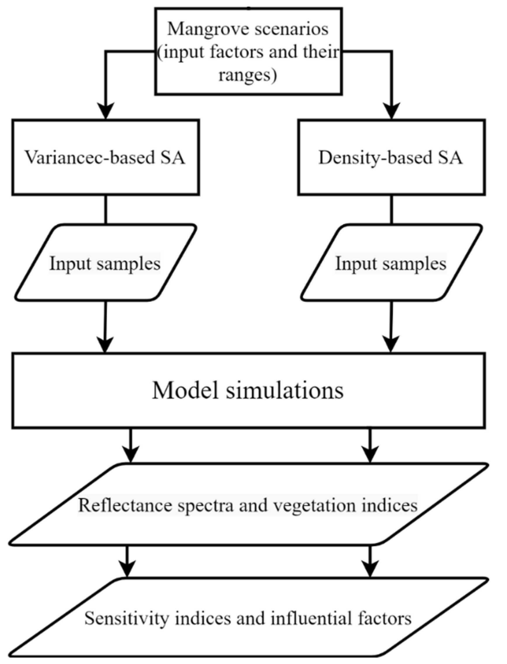
In this study, 16 factors were selected based on a priori knowledge, similar studies such as [19,20,22] and trial tests. As only images captured by nadir or near-nadir viewing satellites, e.g., Sentinel-2, would be applied at this stage, the observation zenith angle was set as 0°, and the solar zenith angle was fixed as 30° to avoid distraction. Then various mangrove scenarios such as sparse or dense canopies were set up according to one or more properties such as the crown PAI and fCv. This corresponded to different mangrove formations such as open or closed forests. Samples of the 16 input factors were generated using VBSA or DBSA and following uniform or normal probability distributions. The canopy reflectance spectra from 400 to 2500 nm with a 1 nm interval were then simulated using a CRM of mangrove [28]. Additionally, values of corresponding S2A bands (Bands 2–8, 8a, 11 and 12) were simulated by convolving the simulated reflectance spectra with the spectral response functions of S2A. Then twelve VIs were calculated. Finally, both VBSA and DBSA were performed and the computed sensitivity indices were examined and compared. The GSA flowchart is shown in Figure 1.
2.2. Canopy Reflectance Model of Mangroves
The adopted CRM of mangroves was a one-dimensional multiple-layer radiative transfer model [28]. It considered essential biophysical and biochemical properties of mangroves such as Cab, PAI, fCv, L2T ratio, inclination distributions of leaves and woody material and environmental factors such as the water body. It could be regarded as an extension of a previous CRM for aquatic vegetation [23], which was a revision of the PROSAIL model. Mangroves were divided into three layers as in [28]: the understory (L1), the stem (L2) and the crown (L3) layers (Figure 2). The layer index would be added to the variable names in the following to distinguish them from each other, e.g., PAI(3) for the PAI of the crown layer. The height of the understory was assumed to be the same as water depth (Hw), and water was not allowed to immerse the crown as that could change canopy reflectance significantly [29]. Stems were assumed to be covered by the crowns and hence only had a minor contribution to canopy reflectance. Thus, the stem layer was assigned a low PAI value of 0.5 and a low fCv value of 0.15, according to [28]. Similarly, most factors with regard to the optically active components in the water body and other environmental factors such as bottom reflectance were also fixed as their impact on canopy reflectance was minor when covered by the canopy. For example, the contribution of suspended particles in the background water on canopy reflectance was around 10% or lower and mainly in the visible region [22,28]. Therefore, more attention was paid to the crown, the understory and Hw, and other factors were beyond the scope of this study. Hw corresponded to the changing tidal height. PAI(1) and fCv(1) were employed to explore if there were any potential contributions from the understory to the observed canopy reflectance, especially for a sparse canopy.
2.3. Mangrove Scenarios
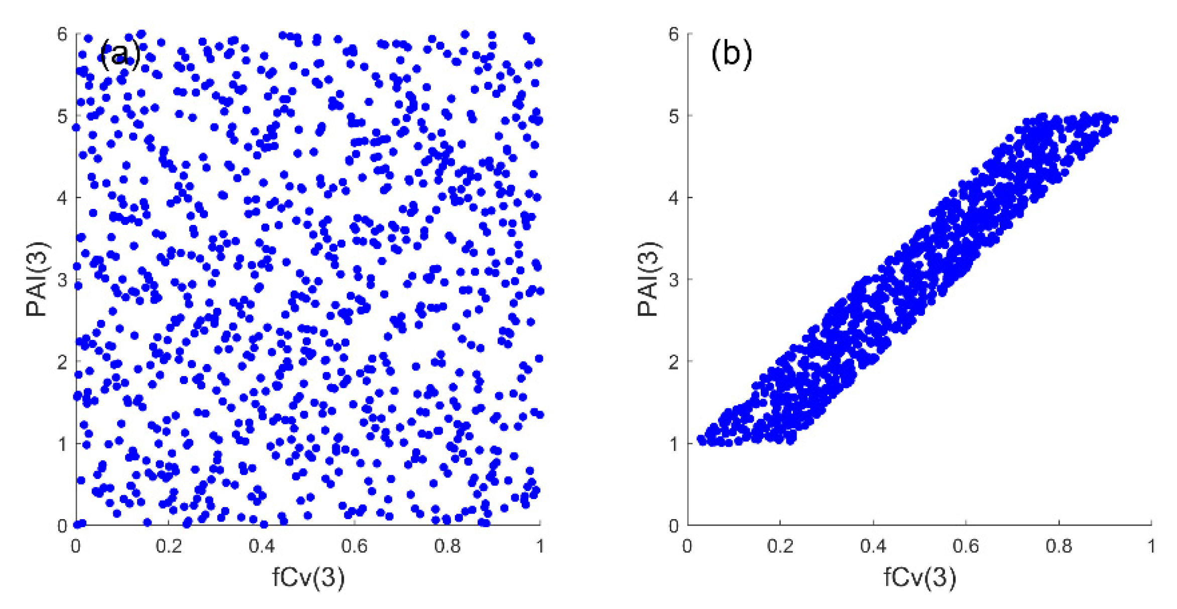
If not specified, the input factors were independent, as they were treated in other SA studies [19,20,22]. All samples discussed in Section 2.3.1 were generated using the Latin hypercube sampling (LHS) [30] following a uniform or normal probability distribution. Although independent input samples were widely adopted in SA studies, there might be an issue with some biophysical properties. For example, it was possible to obtain a high PAI(3) value together with a low fCv(3) value or vice versa if they were assumed to be independent (Figure 3a). However, this was not reasonable in nature and the field data in [28] revealed a positive correlation with a coefficient of determination of 0.73 between the PAI and fCv of mangroves. Therefore, another input dataset with correlated PAI(3) and fCv(3) was also designed in Section 2.3.2.
2.3.1. Factors, Their Ranges and Distributions
GSA was performed for three different mangrove scenarios defined by the ranges of PAI(3) and fCv(3): general canopy (GEN), sparse canopy (SPS) and dense canopy (DEN) (Table 1), as previous studies demonstrated that different ranges of inputs could result in different sensitivity values [19,22]. PAI(3) ranges were set as 0–6 for GEN, 0–3 for SPS and 3–6 for DEN according to the literature [19,31]. Correspondingly, fCv(3) ranges were 0–1, 0–0.7 and 0.5–1. The overlap between the fCv(3) ranges for SPS and DEN was to reflect the variability in mangrove forests. The SPS and DEN scenarios corresponded to open and closed mangrove forests, while the GEN scenario included both situations and implied a significant variation of mangrove formations. Ranges of other factors such as leaf parameters were not changed across these scenarios.
In addition to the GSA methods and ranges of inputs, the probability distributions of inputs might also impact the sensitivity values [32]. The uniform (UNI) and normal (NRM) probability distributions were both adopted for the input factors under SPS and DEN. The mean values for NRM were selected according to [28], and corresponding standard deviation values were set as 10% of the mean values, except for LIDFa(3) and WIDFa(3). NRM indicated that a priori information on the mangrove forest was available and the variability in canopy structure was small, while UNI indicated a larger variation in canopy structure. Under GEN, only a uniform distribution was applied as it might not be suitable to use a nominal value to represent such a wide range of PAI(3).
2.3.2. Correlated PAI(3) and fCv(3)
In this case, the linear relationship between PAI and fCv of mangroves from [28] was applied to generate samples for correlated PAI(3) and fCv(3). First, the ranges of PAI(3) and fCv(3) were set as 1–5 and 0.1–0.9. Hence, their values were within 0–6 and 0–1 after adding random variations. Then random samples of all 16 factors were generated as in the GEN case. Second, PAI(3) or fCv(3) was modified to make them correlated. For VBSA, fCv(3) values were recalculated according to PAI(3) values and the linear relationship, and subsequently, random variations within ±0.1 were added (Figure 3b). In the case of PAWN, the same methodology was used to compute unconditional CDF and conditional CDFs for most factors except fCv(3). When fCv(3) was fixed for computing the corresponding conditional CDFs, PAI(3) was recalculated based on fCv(3), and then a random variation within ±0.8 was given. Finally, sensitivity indices for these two sample datasets were computed using VBSA and PAWN, respectively. Correlated inputs were only applied to GEN as a demonstration because the relationship between PAI and fCv could be different for various sites and species.
2.4. Vegetation Indices
VIs have been broadly applied for mapping the biophysical properties of mangroves such as LAI [2,3,31], but the impact of woody material, fCv and background water was rarely reported. Although a large number of VIs were available [33] (https://www.indexdatabase.de/, accessed on 9 December 2019), this study did not intend to investigate all possible choices. Instead, the VIs in Table 2 were simulated based on the spectral response function of the S2A multispectral instrument to assess their sensitivities to the input factors such as PAI, fCv, L2T ratio and Hw. These indices were either widely applied for terrestrial vegetation such as NDVI [34] and EVI [35] or in particular, proposed for aquatic vegetation such as NDAVI [36]. Some of the VIs for aquatic vegetation included shortwave infrared (SWIR) bands to address the existence of background water, e.g., RGVI [37] and WFI [38].
2.5. Sensitivity Analysis Methods
2.5.1. Variance-Based Sensitivity Analysis
VBSA employed variance to represent sensitivity and attributed the variance of the model output to the variances of input factors. For a model with k independent input factors and a scalar output Y: Y = f(X1, X2, …, Xk), the variance (V(·)) of Y can be decomposed as [14,15]:
The first order indices Si could be represented by the expected reduction in output variance if Xi could be fixed [15]:
where E(·) was the expectation operator and subscripts Xi or X~i indicated that the operation (E(·) or V(·)) was taken over Xi or all factors but Xi. The total order indices could be written as [15]:
Likewise, was the expected reduction in output variance if all input factors but Xi could be fixed. Other partial variances in Equation (1) corresponded to the interactions among input factors, and more details could be found in [15]. Both first and total order indices were broadly used, but this study only focused on total order indices. Due to numerical errors, this approach might produce negative sensitivity indices, usually corresponding to noninfluential factors [7]. Hence, negative values were reset to zero.
Open-source software was available for VBSA, such as SimLab [43] and the SAFE toolbox [44] (https://www.safetoolbox.info/info-and-documentation/, accessed on 7 May 2019). The SAFE toolbox for MATLAB® was employed in this study as it also provided a DBSA method. Trial tests showed that the computed sensitivity indices in VBSA could be affected by the number of samples, especially for NRM. Multiple sample sizes from 16,000 (1000 × 16) to 128,000 (8000 × 16) with an increment of 16,000 were tested for SPS_NRM and DEN_NRM. Finally, 112,000 samples were generated for each VBSA case as the computed sensitivity indices of reflectance spectra were consistent and stable.
2.5.2. Density-Based Sensitivity Analysis
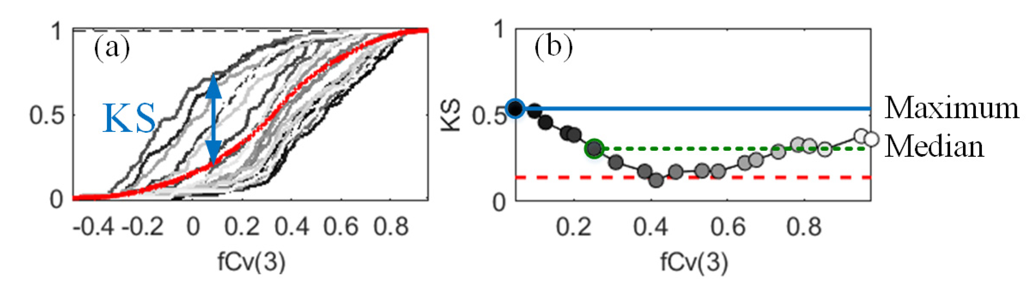
The PAWN method [25] in the SAFE toolbox was adopted for DBSA in this study. It employed output CDFs instead of PDFs to reduce computational costs and to avoid tuning parameters, e.g., the bin width for calculating PDF [25]. The distance between unconditional and conditional output CDFs was taken as a measure of sensitivity. First, Nu samples were randomly generated for a model of k input factors Y = f(X1, X2, … Xk), to evaluate the empirical unconditional CDF of output FY(Y). Second, n samples were generated for each input factor Xi and acted as conditional points. At each conditional point, Nc random samples were generated over X~i to obtain the empirical conditional CDF of output . The Kolmogorov–Smirnov (KS) statistic was applied as a measure of the distance between unconditional and conditional CDFs (as cited in [25]):
In other words, it was the maximum divergence between conditional and unconditional CDFs for a conditional point of Xi. Considering all the conditional points of an input factor Xi, another statistic, e.g., the maximum or the median, was computed over all conditional points of Xi to obtain the PAWN sensitivity index [25]:
By its definition, would be between 0 and 1, and higher values suggested a greater influence on the output [25]. Taking a result for S2A NDVI as an example, the unconditional and conditional CDFs and the KS statistics for all conditioning points of fCv(3) are in Figure 4. As the KS curves had various patterns, derived values using the maximum or the median statistic could be different and thus lead to divergent conclusions. The maximum statistic was adopted because it could detect factors that had influences on the output for at least one conditioning point [32]. The number of samples in a PAWN case was 66,000 in this study, with 2000 samples used to calculate the unconditional CDF, and 20 conditioning points for each of the 16 input factors and 200 samples used per conditioning point. More conditioning points or samples did not change the computed sensitivity indices remarkably.
3. Results
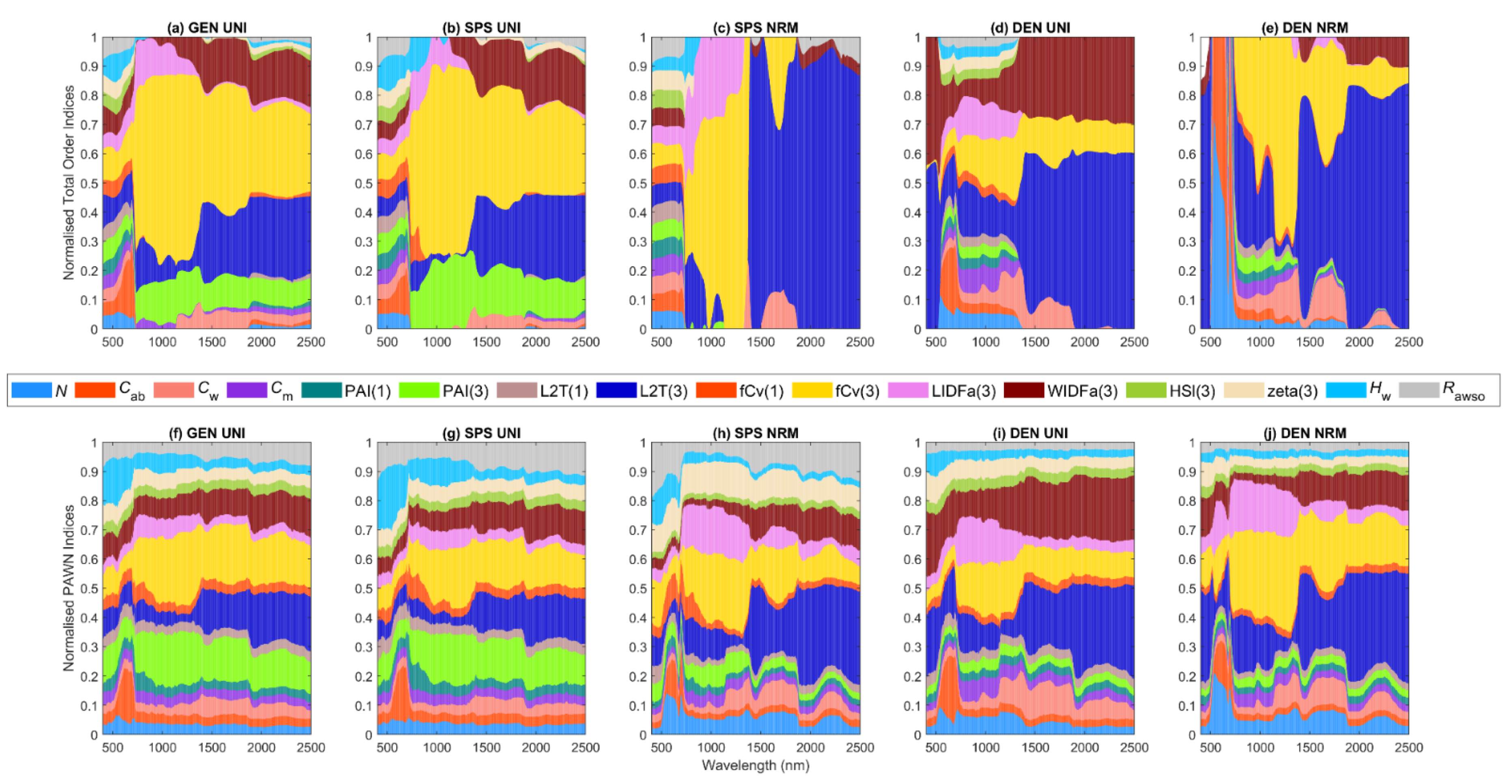
The normalised sensitivity indices (NSIs) for reflectance spectra and sensitivity indices (SIs) for S2A bands and VIs from VBSA and PAWN were presented as stacked bar plots (Figure 5 and Figure 6). As VIs had various scales, they were not normalised to avoid confusion, especially for VBSA indices that sometimes only one or two factors achieved positive sensitivity values, e.g., MDI2 in Figure 6c.
3.1. General Scenario
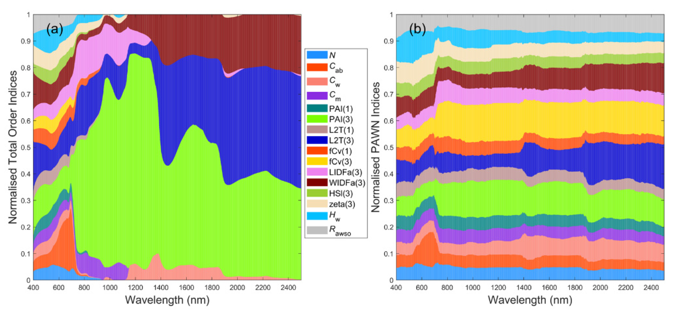
For GEN, two large areas in blue and yellow in Figure 5a could be easily recognised, indicating that L2T(3) and fCv(3) had significant influences on canopy reflectance across nearly the whole visible to SWIR regions in VBSA. Exceptions were the boundaries of chlorophyll absorption bands around 600 nm and 710 nm where the impact of Cab rose and fell abruptly and the NIR bands where the influence of L2T(3) dropped. WIDFa(3) was the next most influential factor, especially in the SWIR, followed by PAI(3) across NIR and SWIR bands. Comparatively, PAWN NSIs were slightly different from VBSA NSIs in that PAI(3) had higher NSI values while the NSI values of L2T(3) and fCv(3) were lower, especially in SWIR (Figure 5f). It is worth noting that Hw had higher NSI values in visible bands compared with its NSI values in other regions.
Since PAWN SIs were always between 0 and 1 while VBSA SIs could have various scales and negative values were reset to zero, the NSI patterns of VIs in the two methods could appear distinct. The stacked PAWN SIs were around 3.5 while stacked VBSA SIs varied from lower than 1 to higher than 6. The scale of the y-axis in Figure 6 was limited to 0–3.8 to maintain sufficient details. Once they were normalised, the length of each bar could be stretched or compressed. Thus, the relative length of the bar for a specific factor might look different in stacked bar plots of SIs and NSIs. In PAWN, multiple VIs had similarly high SI values of fCv(3) such as S2A-B11, MNDWI and RGVI (Figure 6f). A challenge with the PAWN indices was that all factors obtained a SI value between 0 and 1. Hence, the influential factors might look less outstanding than they did in VBSA, even if its SI value was high, e.g., the NSI of fCv(3) for MNDWI was 0.21, but its SI value was 0.68.
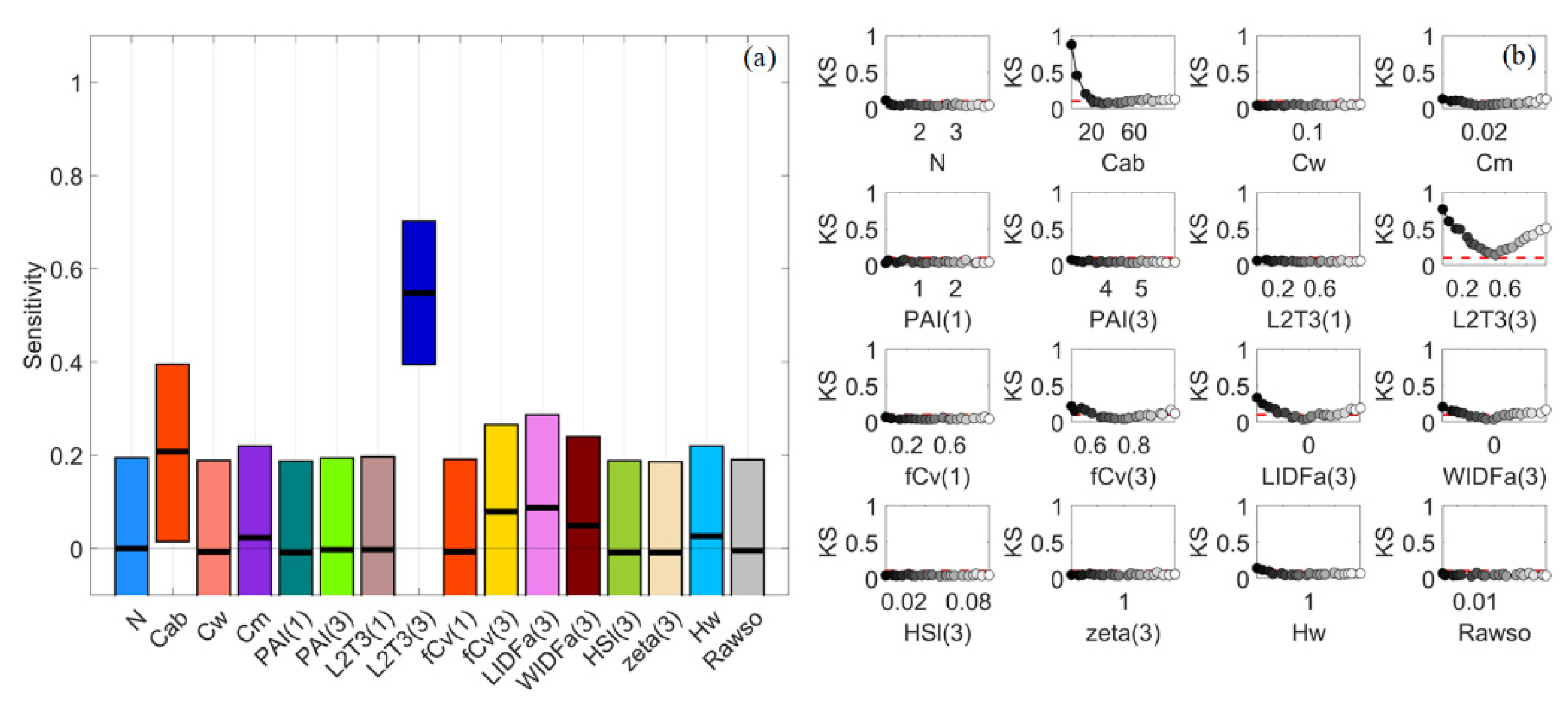
The output PDFs in VBSA were shown in Figure 7. Those outputs that had high NSI or SI values to fCv(3) in VBSA, such as S2A-B8a, MNDWI, NDAVI and RGVI, exhibited various PDFs. Their SIs with confidence intervals were obtained via bootstrapping and further examined. Although the PDF of RGVI was remarkably skewed, all factors had narrow confidence intervals (around 0.1 or lower) and the most influential factor fCv(3) was outstanding (not shown). The confidence intervals were also narrow for MNDWI and NDAVI but were relatively large for S2A-B8a (around 0.25 or higher, Figure 8a). In the case of PAWN, the KS plots for MNDWI with regard to input factors in Figure 8b could provide more insights. KS values of fCv(3) would increase if fCv(3) was approaching 0 or 1 from 0.4 and for the latter case, KS values would become stable after fCv(3) reached about 0.9. When L2T(3) moved towards the two ends 0 or 1, its KS values slightly increased but were not obvious. As for PAI(3) and Hw, their KS values only grew noticeably if their values decreased to zero, e.g., lower than 1 for PAI(3). This implied that PAI(3) was more influential when its value was low.
3.2. Sparse Mangroves—Uniform Input Probability Distributions
The NSIs of reflectance spectra for SPS_UNI had many similarities with those for GEN_UNI, but there was an increased impact of Hw in visible bands (Figure 5b,g). In the NIR region, the NSI values of PAI(1) and fCv(1) slightly increased in PAWN, but only the NSI values of fCv(1) increased in VBSA. This implied that the understory and water background had a larger impact on SPS, which was intuitive. Therefore, more attention was paid to Hw in this section.
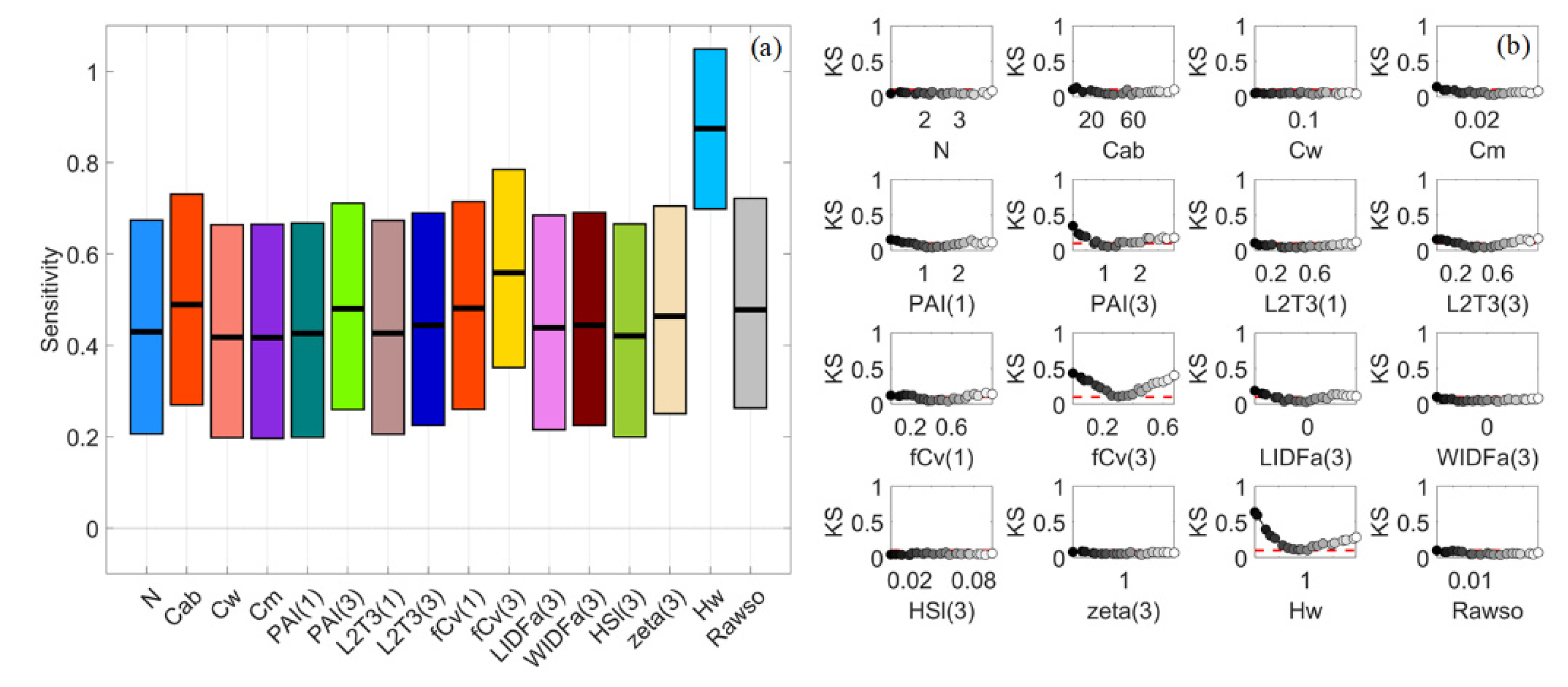
S2A-B3 achieved the highest SI value of 0.87 to Hw, but all factors had large confidence intervals (around 0.4 or higher, Figure 9a). Although Hw could still be distinguished, its bounds were already overlapped with those of other factors. This was somewhat unexpected as the S2A-B3 values were quite normally distributed and far from skewed (Figure 7c). Moreover, a larger sample size of up to 128,000 did not significantly reduce the confidence intervals. For RGVI and NDAVI, Hw, fCv(3) and PAI(3) were all identified as influential, but their SI values slightly varied and their confidence intervals might overlap. For NDWI, the SI of fCv(3) was slightly higher than that of Hw, i.e., 0.360 vs. 0.348. Their confidence intervals were narrow (lower than 0.1) but still overlapping. Ranking them further might not be reliable because of the overlapping confidence intervals [8,45]. Therefore, a high SI itself in VBSA might not guarantee a solid link between the output and an input factor. It was better to check the output distributions and confidence intervals as well, as suggested by [32].
By comparison, S2A-B3 had similar SI patterns in PAWN, with the SI of Hw higher than 0.6 and those of other factors lower than 0.3, but the confidence intervals of all factors were much narrower (around 0.1 or lower). For NDWI, Hw, fCv(3) and PAI(3) had SI values of 0.685, 0.414 and 0.404, separately. All factors had narrow confidence intervals (lower than 0.1) in PAWN, and there was no overlapping between them and other factors. As for the KS plot Figure 9b, PAI(3) and fCv(3) presented similar patterns with those in Figure 8b, except that the KS values of fCv(3) continued rising with increasing fCv(3) since its maximum value was 0.7 rather than 1 in GEN. Hw had a two-way impact on NDWI and S2A-B3. This might be attributed to the different contributions of absorption and scattering by the water body and its components, both of which could vary with water depth. In contrast, only low Hw values could make a difference for VIs based on SWIR bands, e.g., MNDWI in Figure 8b, as the absorption of water in SWIR was strong.
3.3. Sparse Mangroves—Normal Input Probability Distributions
This case corresponded to small variations in the biophysical and biochemical properties of mangrove plots and the environmental factors. As shown in Figure 5b,c, there was a dramatic change in the NSI patterns of reflectance spectra in VBSA. fCv(3) and LIDFa(3) became dominant in NIR, while the most influential factor was L2T(3) in SWIR. Additionally, the impact of other factors was minor in these regions. Consequently, only a limited number of factors obtained positive SIs for multiple VIs such as the EVI and NDVI (Figure 6c). In contrast, the NSI patterns in PAWN also changed but more smoothly (Figure 5h). fCv(3) and L2T(3) were also the most influential factors in NIR and SWIR, separately. In addition, the influences of fCv(1) and LIDFa(3) increased in NIR and the impact of tree shape factor zeta(3) also increased.
As shown in Figure 7, the output PDFs in VBSA for SPS_NRM were remarkably different from those for GEN_UNI and SPS_UNI. This indicated that input distributions could affect the output distributions. However, the normal-like output PDFs did not guarantee that the confidence intervals of SIs were narrow. Taking MNDWI as an example, the confidence intervals were around 0.3, and there was overlapping between influential factors fCv(3) and L2T(3) and other factors (Figure 10a). Comparatively, the confidence intervals for MNDWI (Figure 10b), MDI1 and LSWI in PAWN were basically within 0.1.
3.4. Dense Mangroves—Uniform Input Probability Distributions
When the canopy became dense, the impact of PAI(3) dropped quickly, and the impact of fCv(3) also declined noticeably, as shown by their shrunken areas in Figure 5d,i. Hw barely made a difference in this case. In the meanwhile, the influences of LIDFa(3) increased in NIR and Cw in SWIR. Moreover, the impact of L2T(3) and WIDFa(3) grew significantly, especially in SWIR. L2T(3) had the highest SI values over other factors for multiple VIs such as MDI2, LSWI, NDAVI and WFI (Figure 6d,i). This might be attributed to the distinct spectral responses of leaves and woody material, and the adopted reflectance values of woody material were higher than the reflectance of leaves in SWIR.
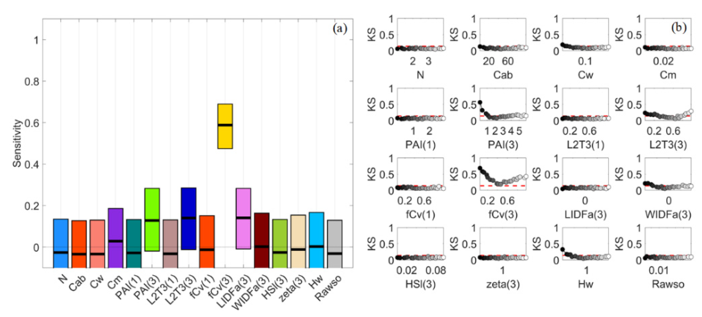
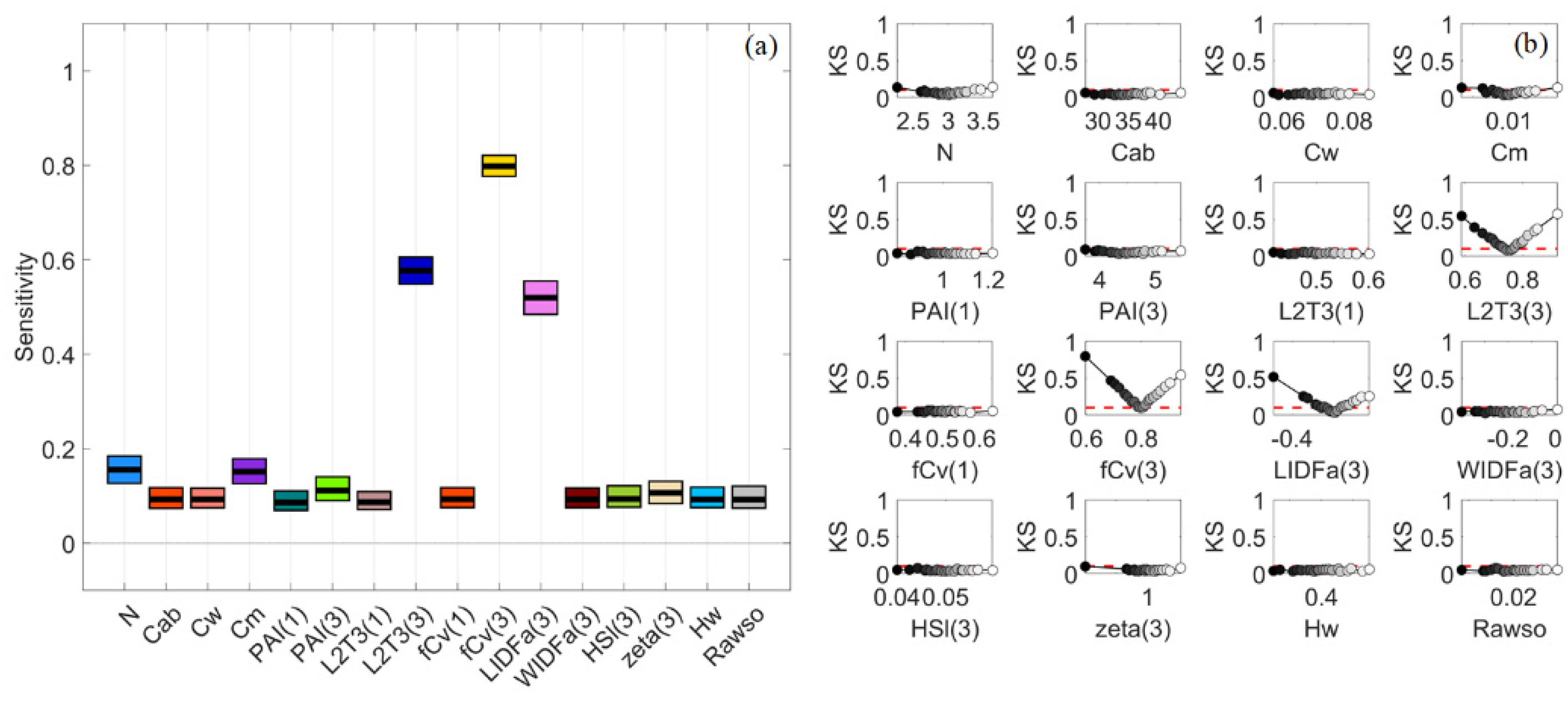
It was interesting to find that Cab also had outstanding PAWN SI values for multiple VIs such as NDVI, EVI and S2A-B4 (Figure 6i). Comparatively, this was less significant for NDVI and EVI in VBSA (Figure 6d). The KS plots for NDVI in PAWN were presented in Figure 11b. L2T(3) had a two-way impact while the KS values of Cab increased dramatically only when its values were lower than 20 μg·cm−2. This was because low Cab values close to zero could remarkably increase the canopy reflectance in chlorophyll absorption bands [46]. The SI values of Cab and L2T(3) for NDVI in PAWN were 0.879 and 0.771, respectively, with SI values of other factors lower than 0.4. The confidence intervals of all factors were within 0.1 in PAWN. In contrast, L2T(3) was the most influential factor (SI = 0.544) for NDVI in VBSA, followed by Cab (SI = 0.207, Figure 11a). However, the confidence intervals were wide (around 0.3 or higher) and overlapping.
3.5. Dense Mangroves—Normal Input Probability Distributions
Compared with the DEN_UNI case (Figure 5d,i), L2T(3) together with fCv(3) still had a dominant impact in NIR and SWIR for DEN_NRM, but L2T(3) was less influential in some NIR bands in VBSA (Figure 5e,j). In addition, LIDFa(3) also had noticeable influences in NIR. WIDFa(3) became less influential compared with that for DEN_UNI. Similar to SPS_NRM, only a limited number of factors had positive SI values in VBSA for multiple VIs such as EVI, MNDWI and WFI (Figure 6e) and the confidence intervals were generally wide (0.25 or higher) in VBSA.
LIDFa(3) was investigated in this section as other influential factors such as fCv(3) and PAI(3) had been covered in previous sections. As shown in Figure 6e,j, NIR bands were the most sensitive to LIDFa(3). Therefore, the KS statistics and confidence intervals for S2A-B8 in PAWN were presented in Figure 12. fCv(3), L2T(3) and LIDFa(3) had high SI values and were distinct from other factors. The KS plots of fCv(3) and L2T(3) in Figure 12b were similar to those in Figure 8b and Figure 9b, indicating that the output CDF diverged from the unconditional CDF when the fCv(3) and L2T(3) values increased or decreased. The KS plot of LIDFa(3) presented a similar pattern to that of fCv(3). Moreover, the KS values were higher when LIDFa(3) moved towards −0.6 (θl = 67°) than they were when LIDFa(3) was close to 0 (θl = 45°), which implied that canopy reflectance in NIR changed more significantly if leaves were vertically distributed.
3.6. General Scenario with Correlated PAI(3) and fCv(3)
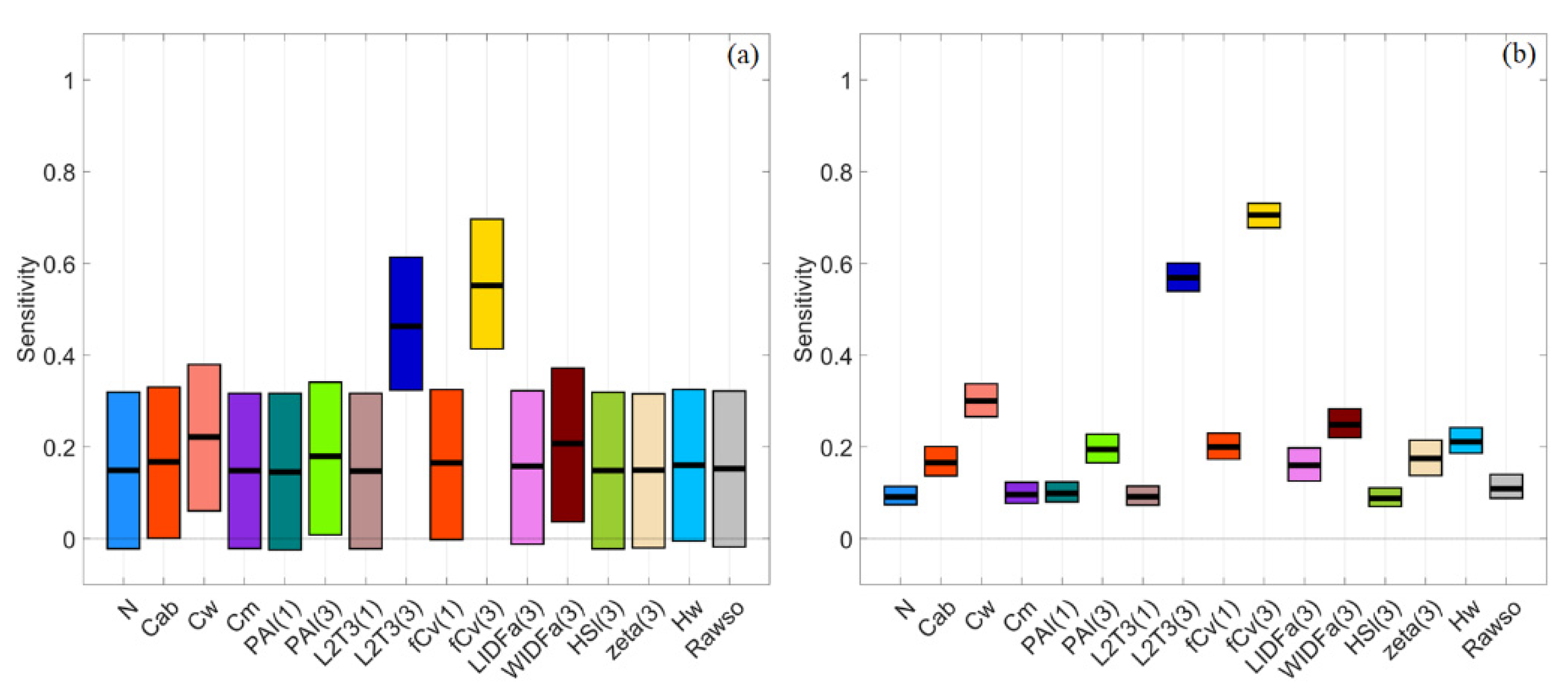
If PAI(3) and fCv(3) were correlated for a general scenario, both were recognised as influential factors in PAWN. Besides, similar NSIs of canopy reflectance could be obtained with the GEN_UNI with random PAI(3) and fCv(3) values (Figure 5f and Figure 13b). In contrast, VBSA only identified PAI(3) as being influential in NIR and SWIR while fCv(3) had virtually no impact (Figure 5a and Figure 13a). The computed NSIs in VBSA in Figure 13a might be meaningless because there were correlated inputs. Thus, no further interpretation was given. This plot demonstrated that the correlated biophysical properties of mangroves changed the calculated sensitivity indices in VBSA.
3.7. A Brief Summary
The results demonstrated the influences of SA methods and input configurations on the calculated SIs for reflectance of mangroves and the importance of examining the confidence intervals of calculated SIs, which might be ignored in previous SA studies on the RS of vegetation. The calculated NSI and SI values highlighted that canopy reflectance of mangroves was sensitive to fCv(3) and L2T(3) and PAI(3). The influences of Hw for a sparse mangrove canopy and inclination distributions of plant material and Cab for a dense canopy might also be noteworthy. VIs with SWIR bands such as MNDWI and RGVI also had potential for mapping the fCv(3) and PAI(3) of mangroves and traditional VIs like EVI. Several VIs such as LSWI, MDI and WFI were sensitive to the L2T(3) of mangroves and might be helpful for estimating the LAI of mangroves from multispectral satellite images.
4. Discussion
4.1. Global Sensitivity Analysis Methods and Interpretations of the Results
The NSIs for canopy reflectance spectra of vegetation, as shown in Figure 5a–e, were frequently adopted in VBSA [19,20,22,47]. In addition, NSIs for VIs were also applied to evaluate the sensitivities of selected VIs to specific biophysical and biochemical properties of vegetation [22,47]. Stacked NSI plots for reflectance spectra were intuitive and straightforward for identifying the most influential factors and corresponding wavelength regions. However, SI values of various VIs could have distinct scales and only a limited number of factors might have non-negative SI values in VBSA, such as EVI and SAVI in Figure 6c. Therefore, a factor could obtain a high and dominant NSI value for a VI, e.g., the NSI of fCv(3) was 0.641 for EVI, while its absolute SI value was only 0.181 and not the highest compared with other VIs. Hence, the NSI values might mislead us to conclude that EVI was the most sensitive to fCv(3) in this case. Moreover, if a VI was only sensitive to a limited number of factors, the confidence intervals of these factors might be large and overlapping, and, thus, the results were not robust.
With regards to the output PDFs in VBSA, the results only showed that input distributions could affect output distributions but did not reveal any promising links between output PDFs and the confidence intervals of calculated SIs. A highly skewed output PDF such as RGVI in Figure 7y for SPS_UNI did not necessarily mean the SIs in VBSA had wide or overlapping confidence intervals. On the other hand, a normal-like output PDF such as S2A-B3 in Figure 7c for SPS_UNI did not guarantee robust SIs in VBSA (Figure 9a). In addition, different numbers of input samples in VBSA did not significantly change the output PDFs as long as they were large enough but could result in divergent SI values in this study, especially for normally distributed input samples. Comparatively, the confidence intervals of calculated SIs for S2A band reflectance and VIs were usually narrow in PAWN with 2000 samples for the unconditional CDF and 200 samples per conditional point by 20 conditional points for conditional CDFs. The KS plots could be used to identify the value ranges of inputs where conditional output CDFs diverged from the unconditional CDF, which implied that there were noticeable changes in the output values.
4.2. Differences between Sparse and Dense Mangrove Canopies
The results also demonstrated that input ranges and distributions could affect the computed SIs, particularly in VBSA. For the GEN_UNI case that PAI varied from 0 to 6, fCv(3), L2T(3) and PAI(3) were recognised as the most influential factors (Figure 5a,f). This partly coincided with the results of [20] that fCv and PAI were among the most influential factors. For the SPS_UNI case, the impact of fCv(3) became slightly less dominant in VBSA while the impact of PAI(3) increased (Figure 5a,b). The changes in the impact of PAI(3) and fCv(3) in PAWN were not significant (Figure 5f,g). Additionally, increased influences of Hw and fCv(1) in visible and NIR bands were identified by both methods. If the inputs were turned into normal distributions (SPS_NRM), the computed NSIs of reflectance spectra also changed remarkably. As shown in Figure 5c,h, PAI(3) became less influential while the impact of fCv(3) and L2T(3) increased in NIR and SWIR, respectively.
If the canopy was dense with uniformly distributed inputs (DEN_UNI), the NSI values of fCv(3) and PAI(3) decreased, particularly for PAI(3) (Figure 5d,i). Factors regarding the understory and background such as PAI(1) and Hw had negligible influence now. In the meanwhile, biophysical properties related to woody material, such as L2T(3) and WIDFa(3), had a dominant impact in SWIR. The impact of LIDFa(3) also grew remarkably in NIR. In addition, the influences of leaf parameters, including Cab, Cw and Cm, increased by various degrees in different spectral regions. For the DEN_NRM case, the NSI patterns in PAWN (Figure 5j) were similar but slightly different from Figure 5i for DEN_UNI. The impact of fCv(3), L2T(3) and LIDFa(3) increased while that of WIDFa(3) decreased. In VBSA, fCv(3) and L2T(3) became the most influential factors, and the influences of LIDFa(3) and WIDFa(3) both decreased (Figure 5e).
In summary, PAI(3) had a larger impact under the sparse canopy while the influences of leaf parameters and inclination angles increased under a dense canopy. This agreed with the results in [19,22]. The new factors fCv(3) and L2T(3) were among the most influential factors under all examined scenarios except for the correlated case where fCv(3) was not identified as influential in VBSA. Hw mainly affected the reflectance of sparse canopies, but it was worth noting that the water body was not allowed to immerse the crown in this study. Otherwise, the infrared reflectance of submerged mangroves would reduce dramatically, which had been used to identify them from satellite images [4,48].
4.3. Potential Limitations and Suggestions
The structure of real mangrove forests was more complicated than the model could simulate. Simplifications in the model might result in overestimated contributions from fCv(3) because it was applied to weight the reflected radiation from mangroves directly. Additionally, the woody material was assumed to be randomly distributed and to share the same fractional cover with leaves in the adopted model [28]. Its reflectance spectra were averaged from field measurements over the lower parts (lower than 2 m) of stems [28], which might be different from the reflectance of branches and shoots in the crowns. Consequently, the contributions of L2T(3) and its SIs could also be overestimated.
Although there were potential divergences in the computed SI values of L2T(3), the impact of woody material on canopy reflectance were demonstrated [5,49]. In addition, caution for the inclination distributions of leaves and wood was still needed because they could be an obstacle when mapping the LAI of mangroves from satellite images. The leaf area ratio could be measured by classifying the point clouds acquired by laser scanning [50,51]. Average inclination angles could also be calculated from point clouds [52,53] or digital photos [54]. However, convenient and operational methods were still lacking [55], particularly when they needed to be measured together with PAI and fCv at many of the plots to be used as calibration or validation data.
For future studies, it might be a good start to map the fCv of mangroves together with PAI because field data of fCv were relatively easy to collect, e.g., by taking hemispherical photos or upward photos [56]. Moreover, the data could be used to assess the potential correlation between PAI and fCv, and further the impact of fCv and background water on PAI mapping. According to the GSA results in this study, multiple VIs may be suitable for mapping PAI and fCv of mangroves from S2A images. Besides traditional VIs such as EVI and NDVI, other VIs such as MNDWI and RGVI were also sensitive to fCv and PAI. The new VIs for mangroves or aquatic plants such as MDI, WFI and RGVI had a common characteristic that SWIR bands were incorporated. This study showed that the SWIR bands and these VIs could be helpful for mapping mangroves, but the optimal VI for mapping a biophysical property from a specific dataset might vary.
5. Conclusions
Based on a canopy reflectance model of mangroves, this study demonstrated that GSA methods (variance-based or density-based), input ranges and probability distributions (uniform or normal) could affect the computed sensitivity indices under the examined mangrove scenarios. Briefly, fCv(3) and L2T(3) were among the influential factors for the infrared reflectance of mangroves under the examined scenarios. PAI(3) was also influential for a sparse canopy but became less influential for a dense canopy. In contrast, inclination distributions of plant material and leaf parameters, e.g., leaf water content, could become more influential in infrared bands for a dense canopy. Moreover, the influence of water depth was noteworthy for a sparse canopy and maybe other scenarios if the water body could immerse the crown.
Since the results and conclusions can be different if a specific model, GSA method and input configuration are adopted, it may be essential to perform a tailored GSA according to the study area and available data. Based on the results, it is recommended that attention should be paid to the L2T and fCv as they may affect estimating the LAI or PAI of mangroves. A complete field dataset that includes the factor to be mapped such as LAI and if possible, other influential factors such as fCv, L2T ratio and inclination angles would be beneficial to further analyses and evaluations of their impact. This, in turn, could contribute to the development of a protocol on field data collection for mapping mangrove from remote sensing images. Considering the challenges in field data collection, it may be a good start to collect and map PAI and fCv of mangroves. For VI based mapping methods, more choices such as MNDWI and RGVI deserve an attempt if SWIR bands are available, but tests are still needed to determine the optimal VI for mapping a specific property based on the available field data and RS images.
Author Contributions
Conceptualization, C.N. and S.P.; Data curation, C.N.; Formal analysis, C.N.; Funding acquisition, C.N. and S.P.; Methodology, C.N.; Project administration, C.N. and S.P.; Resources, C.N. and S.P.; Software, C.N.; Supervision, S.P. and C.R.; Writing—original draft, C.N.; Writing—review and editing, S.P. and C.R. All authors have read and agreed to the published version of the manuscript.
Funding
Chunyue Niu was supported by an Australian Government Research Training Program (RTP) Scholarship and Remote Sensing Research Centre, School of Earth and Environmental Sciences, The University of Queensland.
Institutional Review Board Statement
Not applicable.
Informed Consent Statement
Not applicable.
Data Availability Statement
Not applicable.
Acknowledgments
We thank Francesca Pianosi, Fanny Sarrazin and Thorsten Wagener at the University of Bristol for sharing the SAFE toolbox. We are grateful to the anonymous reviewers for their valuable comments.
Conflicts of Interest
The authors declare no conflict of interest.
References
- Kamal, M.; Phinn, S. Hyperspectral data for mangrove species mapping: A comparison of pixel-based and object-based approach. Remote Sens. 2011, 3, 2222–2242. [Google Scholar] [CrossRef] [Green Version]
- Kovacs, J.M.; Wang, J.; Flores-Verdugo, F. Mapping mangrove leaf area index at the species level using IKONOS and LAI-2000 sensors for the Agua Brava Lagoon, Mexican Pacific. Estuar. Coast. Shelf Sci. 2005, 62, 377–384. [Google Scholar] [CrossRef]
- Heenkenda, M.K.; Maier, S.W.; Joyce, K.E. Estimating Mangrove Biophysical Variables Using WorldView-2 Satellite Data: Rapid Creek, Northern Territory, Australia. J. Imaging 2016, 2, 24. [Google Scholar] [CrossRef] [Green Version]
- Jia, M.; Wang, Z.; Wang, C.; Mao, D.; Zhang, Y. A new vegetation index to detect periodically submerged Mangrove forest using single-tide Sentinel-2 imagery. Remote Sens. 2019, 11, 2043. [Google Scholar] [CrossRef] [Green Version]
- Widlowski, J.-L.; Côté, J.-F.; Béland, M. Abstract tree crowns in 3D radiative transfer models: Impact on simulated open-canopy reflectances. Remote Sens. Environ. 2014, 142, 155–175. [Google Scholar] [CrossRef]
- Cárdenas, N.Y.; Joyce, K.E.; Maier, S.W. Monitoring mangrove forests: Are we taking full advantage of technology? Int. J. Appl. Earth Obs. Geoinf. 2017, 63, 1–14. [Google Scholar] [CrossRef] [Green Version]
- Saltelli, A.; Ratto, M.; Andres, T.; Campolongo, F.; Cariboni, J.; Gatelli, D.; Saisana, M.; Tarantola, S. Global Sensitivity Analysis: The Primer; John Wiley & Sons: Hoboken, NJ, USA, 2008. [Google Scholar]
- Pianosi, F.; Beven, K.; Freer, J.; Hall, J.W.; Rougier, J.; Stephenson, D.B.; Wagener, T. Sensitivity analysis of environmental models: A systematic review with practical workflow. Environ. Model. Softw. 2016, 79, 214–232. [Google Scholar] [CrossRef]
- Jacquemoud, S.; Baret, F. PROSPECT: A model of leaf optical properties spectra. Remote Sens. Environ. 1990, 34, 75–91. [Google Scholar] [CrossRef]
- Verhoef, W. Light scattering by leaf layers with application to canopy reflectance modeling: The SAIL model. Remote Sens. Environ. 1984, 16, 125–141. [Google Scholar] [CrossRef] [Green Version]
- Verhoef, W. Theory of Radiative Transfer Models Applied in Optical Remote Sensing of Vegetation Canpioes. Ph.D. Thesis, Wageningen Agricultural University, Wageningen, The Netherlands, 1998. [Google Scholar]
- Verhoef, W.; Bach, H. Coupled soil–leaf-canopy and atmosphere radiative transfer modeling to simulate hyperspectral multi-angular surface reflectance and TOA radiance data. Remote Sens. Environ. 2007, 109, 166–182. [Google Scholar] [CrossRef]
- Jacquemoud, S.; Verhoef, W.; Baret, F.; Bacour, C.; Zarco-Tejada, P.J.; Asner, G.P.; François, C.; Ustin, S.L. PROSPECT+ SAIL models: A review of use for vegetation characterization. Remote Sens. Environ. 2009, 113, S56–S66. [Google Scholar] [CrossRef]
- Sobol, I.M. Global sensitivity indices for nonlinear mathematical models and their Monte Carlo estimates. Math. Comput. Simul. 2001, 55, 271–280. [Google Scholar] [CrossRef]
- Saltelli, A.; Annoni, P.; Azzini, I.; Campolongo, F.; Ratto, M.; Tarantola, S. Variance based sensitivity analysis of model output. Design and estimator for the total sensitivity index. Comput. Phys. Commun. 2010, 181, 259–270. [Google Scholar] [CrossRef]
- Liu, J.; Pattey, E.; Jégo, G. Assessment of vegetation indices for regional crop green LAI estimation from Landsat images over multiple growing seasons. Remote Sens. Environ. 2012, 123, 347–358. [Google Scholar] [CrossRef]
- Saltelli, A.; Tarantola, S.; Chan, K.-S. A quantitative model-independent method for global sensitivity analysis of model output. Technometrics 1999, 41, 39–56. [Google Scholar] [CrossRef]
- Campbell, G. Derivation of an angle density function for canopies with ellipsoidal leaf angle distributions. Agric. For. Meteorol. 1990, 49, 173–176. [Google Scholar] [CrossRef]
- Xiao, Y.; Zhao, W.; Zhou, D.; Gong, H. Sensitivity analysis of vegetation reflectance to biochemical and biophysical variables at leaf, canopy, and regional scales. IEEE Trans. Geosci. Remote Sens. 2014, 52, 4014–4024. [Google Scholar] [CrossRef]
- Mousivand, A.; Menenti, M.; Gorte, B.; Verhoef, W. Global sensitivity analysis of the spectral radiance of a soil–vegetation system. Remote Sens. Environ. 2014, 145, 131–144. [Google Scholar] [CrossRef]
- Villa, P.; Mousivand, A.; Bresciani, M. Aquatic vegetation indices assessment through radiative transfer modeling and linear mixture simulation. Int. J. Appl. Earth Obs. Geoinf. 2014, 30, 113–127. [Google Scholar] [CrossRef]
- Zhou, G.; Ma, Z.; Sathyendranath, S.; Platt, T.; Jiang, C.; Sun, K. Canopy Reflectance Modeling of Aquatic Vegetation for Algorithm Development: Global Sensitivity Analysis. Remote Sens. 2018, 10, 837. [Google Scholar] [CrossRef] [Green Version]
- Zhou, G.; Niu, C.; Xu, W.; Yang, W.; Wang, J.; Zhao, H. Canopy modeling of aquatic vegetation: A radiative transfer approach. Remote Sens. Environ. 2015, 163, 186–205. [Google Scholar] [CrossRef]
- Saltelli, A. Sensitivity analysis for importance assessment. Risk Anal. 2002, 22, 579–590. [Google Scholar] [CrossRef]
- Pianosi, F.; Wagener, T. A simple and efficient method for global sensitivity analysis based on cumulative distribution functions. Environ. Model. Softw. 2015, 67, 1–11. [Google Scholar] [CrossRef] [Green Version]
- Borgonovo, E.; Tarantola, S. Moment independent and variance-based sensitivity analysis with correlations: An application to the stability of a chemical reactor. Int. J. Chem. Kinet. 2008, 40, 687–698. [Google Scholar] [CrossRef]
- Borgonovo, E.; Plischke, E. Sensitivity analysis: A review of recent advances. Eur. J. Oper. Res. 2016, 248, 869–887. [Google Scholar] [CrossRef]
- Niu, C. Canopy Reflectance Modelling for Mapping Coastal Wetland Vegetation of South East Queensland, Australia. Ph.D. Thesis, The University of Queensland, Brisbane, Australia, 2021. [Google Scholar]
- Kearney, M.S.; Stutzer, D.; Turpie, K.; Stevenson, J.C. The effects of tidal inundation on the reflectance characteristics of coastal marsh vegetation. J. Coast. Res. 2009, 25, 1177–1186. [Google Scholar] [CrossRef]
- McKay, M.D.; Beckman, R.J.; Conover, W.J. Comparison of three methods for selecting values of input variables in the analysis of output from a computer code. Technometrics 1979, 21, 239–245. [Google Scholar]
- Kamal, M.; Phinn, S.; Johansen, K. Assessment of multi-resolution image data for mangrove leaf area index mapping. Remote Sens. Environ. 2016, 176, 242–254. [Google Scholar] [CrossRef]
- Noacco, V.; Sarrazin, F.; Pianosi, F.; Wagener, T. Matlab/R workflows to assess critical choices in Global Sensitivity Analysis using the SAFE toolbox. MethodsX 2019, 6, 2258–2280. [Google Scholar] [CrossRef]
- Henrich, V.; Götze, E.; Jung, A.; Sandow, C.; Thürkow, D.; Gläßer, C. Development of an Online indices-database: Motivation, concept and implementation. In Proceedings of the 6th EARSeL Imaging Spectroscopy SIG Workshop Innovative Tool for Scientific and Commercial Environment Applications, Tel Aviv, Israel, 16–18 March 2009. [Google Scholar]
- Rouse, J.W.; Haas, R.H.; Schell, J.A.; Deering, D.W.; Harlan, J.C. Monitoring the vernal advancement and retrogradation (green wave effect) of natural vegetation. In NASA/GSFCT Type III Final Report; Greenbelt, MD, USA, 1974. [Google Scholar]
- Huete, A.R.; Liu, H.Q.; Batchily, K.V.; Van Leeuwen, W. A comparison of vegetation indices over a global set of TM images for EOS-MODIS. Remote Sens. Environ. 1997, 59, 440–451. [Google Scholar] [CrossRef]
- Villa, P.; Laini, A.; Bresciani, M.; Bolpagni, R. A remote sensing approach to monitor the conservation status of lacustrine Phragmites australis beds. Wetl. Ecol. Manag. 2013, 21, 399–416. [Google Scholar] [CrossRef]
- Nuarsa, I.W.; Nishio, F.; Hongo, C. Spectral characteristics and mapping of rice plants using multi-temporal Landsat data. J. Agric. Sci. 2011, 3, 54. [Google Scholar] [CrossRef] [Green Version]
- Wang, D.; Wan, B.; Qiu, P.; Su, Y.; Guo, Q.; Wang, R.; Sun, F.; Wu, X. Evaluating the Performance of Sentinel-2, Landsat 8 and Pléiades-1 in Mapping Mangrove Extent and Species. Remote Sens. 2018, 10, 1468. [Google Scholar] [CrossRef] [Green Version]
- Huete, A.R. A soil-adjusted vegetation index (SAVI). Remote Sens. Environ. 1988, 25, 295–309. [Google Scholar] [CrossRef]
- McFeeters, S.K. The use of the Normalized Difference Water Index (NDWI) in the delineation of open water features. Int. J. Remote Sens. 1996, 17, 1425–1432. [Google Scholar] [CrossRef]
- Xu, H. Modification of normalised difference water index (NDWI) to enhance open water features in remotely sensed imagery. Int. J. Remote Sens. 2006, 27, 3025–3033. [Google Scholar] [CrossRef]
- Xiao, X.; Boles, S.; Liu, J.; Zhuang, D.; Frolking, S.; Li, C.; Salas, W.; Moore, B. Mapping paddy rice agriculture in southern China using multi-temporal MODIS images. Remote Sens. Environ. 2005, 95, 480–492. [Google Scholar] [CrossRef]
- Tarantola, S.; Becker, W. SIMLAB Software for Uncertainty and Sensitivity Analysis. In Handbook of Uncertainty Quantification; Ghanem, R., Higdon, D., Owhadi, H., Eds.; Springer: New York, NY, USA, 2015. [Google Scholar]
- Sarrazin, F.; Pianosi, F.; Wagener, T. An Introduction to the SAFE Matlab Toolbox With Practical Examples and Guidelines. In Sensitivity Analysis in Earth Observation Modelling; Petropoulos, G., Srivastava, P.K., Eds.; Elsevier: Amsterdam, The Netherlands, 2017; pp. 363–378. [Google Scholar]
- Vanuytrecht, E.; Raes, D.; Willems, P. Global sensitivity analysis of yield output from the water productivity model. Environ. Model. Softw. 2014, 51, 323–332. [Google Scholar] [CrossRef] [Green Version]
- Jacquemoud, S. Inversion of the PROSPECT+ SAIL canopy reflectance model from AVIRIS equivalent spectra: Theoretical study. Remote Sens. Environ. 1993, 44, 281–292. [Google Scholar] [CrossRef]
- Morcillo-Pallarés, P.; Rivera-Caicedo, J.P.; Belda, S.; De Grave, C.; Burriel, H.; Moreno, J.; Verrelst, J. Quantifying the Robustness of Vegetation Indices through Global Sensitivity Analysis of Homogeneous and Forest Leaf-Canopy Radiative Transfer Models. Remote Sens. 2019, 11, 2418. [Google Scholar] [CrossRef] [Green Version]
- Zhang, X.; Treitz, P.M.; Chen, D.; Quan, C.; Shi, L.; Li, X. Mapping mangrove forests using multi-tidal remotely-sensed data and a decision-tree-based procedure. Int. J. Appl. Earth Obs. Geoinf. 2017, 62, 201–214. [Google Scholar] [CrossRef]
- Malenovský, Z.; Martin, E.; Homolová, L.; Gastellu-Etchegorry, J.-P.; Zurita-Milla, R.; Schaepman, M.E.; Pokorný, R.; Clevers, J.G.; Cudlín, P. Influence of woody elements of a Norway spruce canopy on nadir reflectance simulated by the DART model at very high spatial resolution. Remote Sens. Environ. 2008, 112, 1–18. [Google Scholar] [CrossRef] [Green Version]
- Ma, L.; Zheng, G.; Eitel, J.U.; Magney, T.S.; Moskal, L.M. Determining woody-to-total area ratio using terrestrial laser scanning (TLS). Agric. For. Meteorol. 2016, 228, 217–228. [Google Scholar] [CrossRef] [Green Version]
- Li, Z.; Strahler, A.; Schaaf, C.; Jupp, D.; Schaefer, M.; Olofsson, P. Seasonal change of leaf and woody area profiles in a midlatitude deciduous forest canopy from classified dual-wavelength terrestrial lidar point clouds. Agric. For. Meteorol. 2018, 262, 279–297. [Google Scholar] [CrossRef]
- Bailey, B.N.; Mahaffee, W.F. Rapid measurement of the three-dimensional distribution of leaf orientation and the leaf angle probability density function using terrestrial LiDAR scanning. Remote Sens. Environ. 2017, 194, 63–76. [Google Scholar] [CrossRef] [Green Version]
- Vicari, M.B.; Pisek, J.; Disney, M. New estimates of leaf angle distribution from terrestrial LiDAR: Comparison with measured and modelled estimates from nine broadleaf tree species. Agric. For. Meteorol. 2019, 264, 322–333. [Google Scholar] [CrossRef]
- Qi, J.; Xie, D.; Li, L.; Zhang, W.; Mu, X.; Yan, G. Estimating Leaf Angle Distribution From Smartphone Photographs. IEEE Geosci. Remote Sens. Lett. 2019, 16, 1190–1194. [Google Scholar] [CrossRef]
- Yan, G.; Hu, R.; Luo, J.; Weiss, M.; Jiang, H.; Mu, X.; Xie, D.; Zhang, W. Review of indirect optical measurements of leaf area index: Recent advances, challenges, and perspectives. Agric. For. Meteorol. 2019, 265, 390–411. [Google Scholar] [CrossRef]
- Weiss, M.; Baret, F. CAN_EYE V6.4.91 User Manual; INRA-UMR: Avignon, France, 2017. [Google Scholar]
Figure 1.
The flowchart of global sensitivity analyses for mangroves.

Figure 2.
Illustrations of the understory (L1), stem (L2) and crown (L3) layers for mangroves. Hw is the water depth and is assumed to be the same as the height of the understory for simplicity (The symbols are courtesy of the Integration and Application Network, University of Maryland Center for Environmental Science (ian.umces.edu/symbols/, accessed on 14 June 2018)).

Figure 3.
Illustrations of generated samples (N = 1000) if the crown plant area index (PAI(3)) and fractional cover (fCv(3)) are assumed to be independent (using Latin hypercube sampling) (a) or linearly correlated (b).
Figure 3.
Illustrations of generated samples (N = 1000) if the crown plant area index (PAI(3)) and fractional cover (fCv(3)) are assumed to be independent (using Latin hypercube sampling) (a) or linearly correlated (b).

Figure 4.
Unconditional (red) and conditional (grey) cumulative distribution functions (a) and corresponding Kolmogorov–Smirnov (KS) statistics (b) of the normalised difference vegetation index with regard to the fractional cover of the mangrove crown (fCv(3)). The PAWN index can be different if the maximum (blue) or the median (green) metric is adopted (b).

Figure 5.
Stacked bar plots for normalised sensitivity indices (NSIs) of reflectance spectra in VBSA (a–e) and PAWN (f–j) for a general (GEN) canopy with uniformly sampled inputs (UNI) (a,f), a sparse (SPS) canopy with UNI (b,g), SPS with normally sampled inputs (NRM) (c,h), a dense (DEN) canopy with UNI (d,i) and DEN with NRM (e,j). Each x value corresponds to a wavelength. The NSI value is represented by the height of a bar and marked in the y-axis. Each colour corresponds to a factor defined in Table 1.

Figure 6.
Stacked bar plots for sensitivity indices (SIs) of Sentinel-2A (S2A) band reflectance and vegetation indices (VIs) in VBSA (a–e) and PAWN (f–j) for a general (GEN) canopy with uniformly sampled inputs (UNI) (a,f), a sparse (SPS) canopy with UNI (b,g), SPS with normally sampled inputs (NRM) (c,h), a dense (DEN) canopy with UNI (d,i) and DEN with NRM (e,j). Each x value corresponds to a S2A band reflectance or a VI. The SI value is represented by the height of a bar and marked in the y-axis. The scale of the y-axis is restricted from 0 to 3.8 to show sufficient details. Each colour corresponds to a factor defined in Table 1.

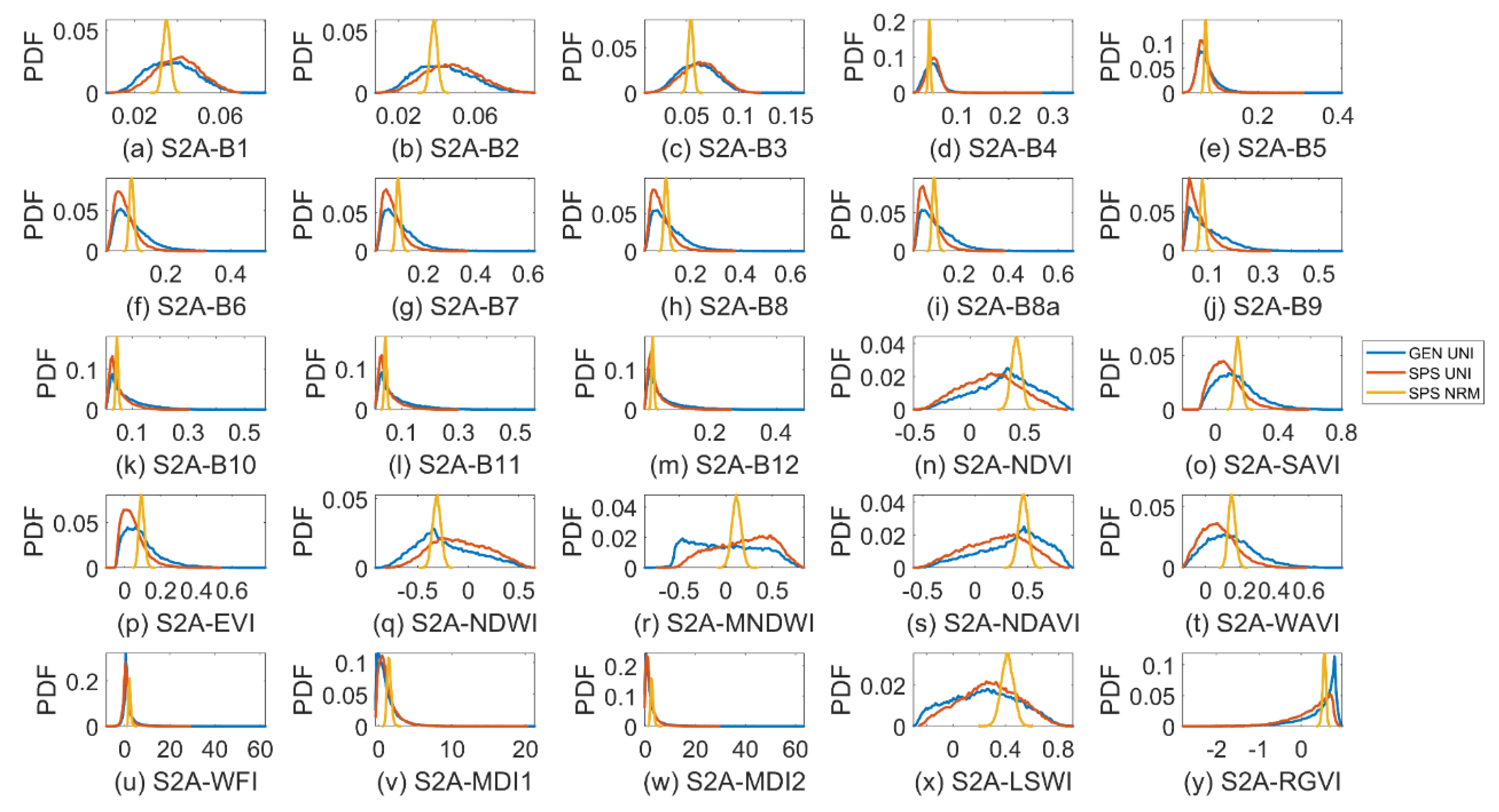
Figure 7.
Probability density function (PDF) of Sentinel-2A (S2A) band reflectance and vegetation indices for a general (GEN) canopy with uniformly sampled inputs (UNI) (blue curves), a sparse (SPS) canopy with UNI (red curves) and SPS with normally sampled inputs (NRM) (yellow curves). The bin size for SPS_NRM is one-third of that for GEN_UNI and SPS_UNI to show details of the latter two.

Figure 8.
Mean sensitivity indices and confidence intervals estimated via bootstrapping for S2A-B8a in VBSA (a). Kolmogorov–Smirnov (KS) statistics for MNDWI with regard to input factors in PAWN (b).
Figure 8.
Mean sensitivity indices and confidence intervals estimated via bootstrapping for S2A-B8a in VBSA (a). Kolmogorov–Smirnov (KS) statistics for MNDWI with regard to input factors in PAWN (b).

Figure 9.
Mean sensitivity indices and confidence intervals estimated via bootstrapping for S2A-B3 in VBSA (a). Kolmogorov–Smirnov (KS) statistics for NDWI with regard to input factors in PAWN (b).
Figure 9.
Mean sensitivity indices and confidence intervals estimated via bootstrapping for S2A-B3 in VBSA (a). Kolmogorov–Smirnov (KS) statistics for NDWI with regard to input factors in PAWN (b).

Figure 10.
Mean sensitivity indices and confidence intervals estimated via bootstrapping for MNDWI in VBSA (a) and PAWN (b).
Figure 10.
Mean sensitivity indices and confidence intervals estimated via bootstrapping for MNDWI in VBSA (a) and PAWN (b).

Figure 11.
Mean sensitivity indices and confidence intervals estimated via bootstrapping for NDVI in VBSA (a). Kolmogorov–Smirnov (KS) statistics for NDVI with regard to input factors in PAWN (b).
Figure 11.
Mean sensitivity indices and confidence intervals estimated via bootstrapping for NDVI in VBSA (a). Kolmogorov–Smirnov (KS) statistics for NDVI with regard to input factors in PAWN (b).

Figure 12.
Mean sensitivity indices and confidence intervals estimated via bootstrapping for S2A-B8 (a) and Kolmogorov–Smirnov (KS) statistics for S2A-B8 with regard to input factors (b) in PAWN.
Figure 12.
Mean sensitivity indices and confidence intervals estimated via bootstrapping for S2A-B8 (a) and Kolmogorov–Smirnov (KS) statistics for S2A-B8 with regard to input factors (b) in PAWN.

Figure 13.
Stacked bar plots for normalised sensitivity indices of reflectance spectra in VBSA (a) and PAWN (b) for a general canopy with correlated PAI(3) and fCv(3). Each x value corresponds to an output, e.g., reflectance or VI, and each colour represents an input factor. The SI value is represented by the height of a bar and marked in the y-axis.


Table 1.
Considered input factors and configurations for mangrove scenarios.
| Factors | Unit | Definitions | General Uniform | Sparse Uniform | Sparse Normal | Dense Uniform | Dense Normal | |||||
|---|---|---|---|---|---|---|---|---|---|---|---|---|
| Min | Max | Min | Max | Mean | STD | Min | Max | Mean | STD | |||
| Leaf | ||||||||||||
| N | - | Leaf structural properties | 1 | 4 | 1 | 4 | 3 | 0.3 | 1 | 4 | 3 | 0.3 |
| Cab | μg∙cm−2 | Leaf chlorophyll content | 0 | 100 | 0 | 100 | 35 | 3.5 | 0 | 100 | 35 | 3.5 |
| Cw | μg∙cm−2 | Leaf water content | 0 | 0.2 | 0 | 0.2 | 0.07 | 0.007 | 0 | 0.2 | 0.07 | 0.007 |
| Cm | g∙cm−2 | Leaf dry matter content | 0 | 0.05 | 0 | 0.05 | 0.01 | 0.001 | 0 | 0.05 | 0.01 | 0.001 |
| Canopy | ||||||||||||
| PAI(1) | - | Plant area index (PAI) of Layer 1 (L1, understory) | 0 | 3 | 0 | 3 | 1 | 0.1 | 0 | 3 | 1 | 0.1 |
| PAI(3) | - | PAI of Layer 3 (L3, crown) | 0 | 6 | 0 | 3 | 2 | 0.2 | 3 | 6 | 4.5 | 0.45 |
| L2T(1) | - | Leaf-to-total area ratio of L1 | 0 | 1 | 0 | 1 | 0.5 | 0.05 | 0 | 1 | 0.5 | 0.05 |
| L2T(3) | - | Leaf-to-total area ratio of L3 | 0 | 1 | 0 | 1 | 0.75 | 0.075 | 0 | 1 | 0.75 | 0.075 |
| fCv(1) | - | Fractional cover of L1 | 0 | 1 | 0 | 1 | 0.5 | 0.05 | 0 | 1 | 0.5 | 0.05 |
| fCv(3) | - | Fractional cover of L3 | 0 | 1 | 0 | 0.7 | 0.3 | 0.03 | 0.5 | 1 | 0.8 | 0.08 |
| LIDFa(3) | - | Leaf inclination distribution function parameter a of L3 a | −1 | 1 | −1 | 1 | −0.2 | 0.1 | −1 | 1 | −0.2 | 0.1 |
| WIDFa(3) | - | Wood inclination distribution function parameter a of L3 | −1 | 1 | −1 | 1 | −0.2 | 0.1 | −1 | 1 | −0.2 | 0.1 |
| HSl(3) | - | Hot spot size parameter of L3 | 0 | 0.1 | 0 | 0.1 | 0.05 | 0.005 | 0 | 0.1 | 0.05 | 0.005 |
| zeta(3) | - | Tree shape factor of L3 | 0 | 2 | 0 | 2 | 1 | 0.1 | 0 | 2 | 1 | 0.1 |
| Other | ||||||||||||
| Hw | m | Water depth | 0 | 2 | 0 | 2 | 0.4 | 0.04 | 0 | 2 | 0.4 | 0.04 |
| Raw_so | - | Bidirectional reflectance of water surface | 0 | 0.03 | 0 | 0.03 | 0.02 | 0.002 | 0 | 0.03 | 0.02 | 0.002 |
Note: Uniform or normal is the probability distribution of input factors, with Min and Max for minimum and maximum values and Mean and STD for mean value and standard deviation. a Equivalent to average inclination angle (AIA) by a = (45 − AIA)∗π2/360 [11].
Table 2.
Definitions and sources of the adopted vegetation indices in this study.
| Indices | Descriptions | References |
|---|---|---|
| NDVI | Normalised Difference Vegetation Index | [34] |
| SAVI | Soil Adjusted Vegetation Index (L: 0–1) | [39] |
| EVI | Enhanced Vegetation Index (G = 2.5, L = 1, C1 = 6, C2 = 7.5) | [35] |
| NDWI | Normalised Difference Water Index | [40] |
| MNDWI | Modified Normalised Difference Water Index | [41] |
| NDAVI | Normalised Difference Aquatic Vegetation Index | [36] |
| WAVI | Water Adjusted Vegetation Index (L: 0–1) | [21] |
| WFI | Wetland Forest Index | [38] |
| MDI1 MDI2 | Mangrove Discrimination Index using SWIR 1 or SWIR2 | [38] |
| LSWI | Land Surface Water Index | [42] |
| RGVI | Rice Growth Vegetation Index | [37] |
Publisher’s Note: MDPI stays neutral with regard to jurisdictional claims in published maps and institutional affiliations. |
© 2021 by the authors. Licensee MDPI, Basel, Switzerland. This article is an open access article distributed under the terms and conditions of the Creative Commons Attribution (CC BY) license (https://creativecommons.org/licenses/by/4.0/).
Share and Cite
MDPI and ACS Style
Niu, C.; Phinn, S.; Roelfsema, C. Global Sensitivity Analysis for Canopy Reflectance and Vegetation Indices of Mangroves. Remote Sens. 2021, 13, 2617. https://0-doi-org.brum.beds.ac.uk/10.3390/rs13132617
AMA Style
Niu C, Phinn S, Roelfsema C. Global Sensitivity Analysis for Canopy Reflectance and Vegetation Indices of Mangroves. Remote Sensing. 2021; 13(13):2617. https://0-doi-org.brum.beds.ac.uk/10.3390/rs13132617
Chicago/Turabian StyleNiu, Chunyue, Stuart Phinn, and Chris Roelfsema. 2021. "Global Sensitivity Analysis for Canopy Reflectance and Vegetation Indices of Mangroves" Remote Sensing 13, no. 13: 2617. https://0-doi-org.brum.beds.ac.uk/10.3390/rs13132617
Note that from the first issue of 2016, this journal uses article numbers instead of page numbers. See further details here.