Author Contributions
Conceptualization, H.H., X.X., Y.G. and G.L.; funding acquisition, H.H., L.M. and G.L.; experiments, X.X., Y.G., G.L. and S.X.; method, X.X., Y.G., G.L. and S.X.; data analysis, X.X., Y.G., G.L. and S.X.; writing, X.X., Y.G., G.L. and S.X. All authors have read and agreed to the published version of the manuscript.
Figure 1.
Sound propagation structure and layer division. Two sound transceivers are deployed in the water and transmit sound reciprocally. Sound waves are reflected by the interface, where multi-path sound propagation is achieved. (a) Sound speed profile. (b) Corresponding acoustic rays.
Figure 1.
Sound propagation structure and layer division. Two sound transceivers are deployed in the water and transmit sound reciprocally. Sound waves are reflected by the interface, where multi-path sound propagation is achieved. (a) Sound speed profile. (b) Corresponding acoustic rays.
Figure 2.
The vertical grid division. The vertical slice is divided into different grids, sound rays propagate across the grids, and water parameter information is taken away. More unknown parameters are introduced in this case.
Figure 2.
The vertical grid division. The vertical slice is divided into different grids, sound rays propagate across the grids, and water parameter information is taken away. More unknown parameters are introduced in this case.
Figure 3.
The left figure shows a map of the Huangcai Reservoir and adjacent regions. The southeast part of Huangcai Reservoir is magnified in the right figure, which shows the position of CAT stations (S1, S2, S3), the point of the TD, and the routes of ADCP sailings. The green solid lines are the projection of acoustic ray paths in the horizontal slice. The upper-right corner of the magnified figure is a photo of the CAT system used at station S1.
Figure 4.
Layout of the three sound stations, including anchored ships, floating balls, additional weights, and CAT systems. The depth of the transceivers and the distance between the stations are shown in
Table 1.
Figure 4.
Layout of the three sound stations, including anchored ships, floating balls, additional weights, and CAT systems. The depth of the transceivers and the distance between the stations are shown in
Table 1.
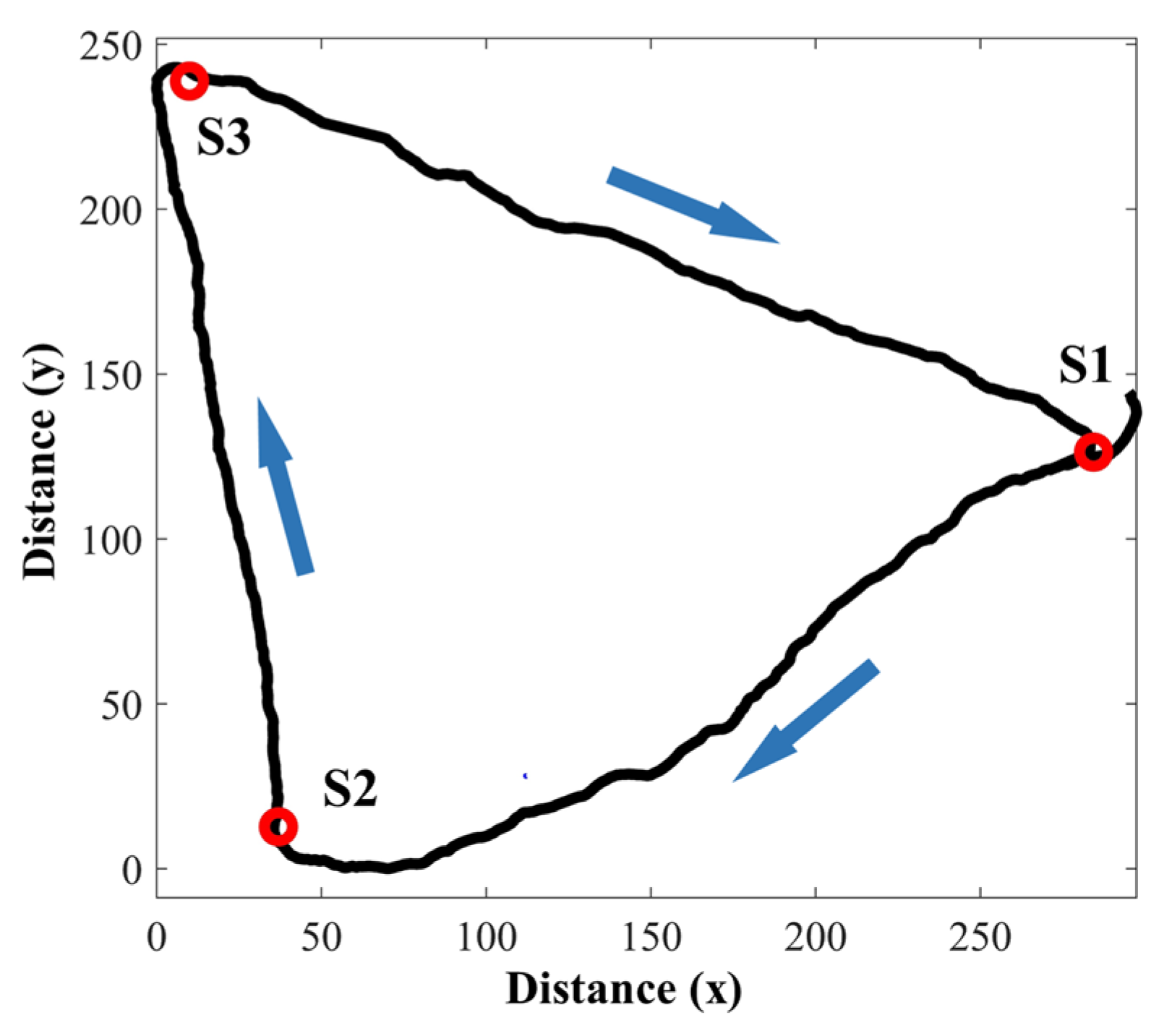
Figure 5.
Sailing route of the ADCP mounted boat, moving clockwise along the blue arrows.
Figure 5.
Sailing route of the ADCP mounted boat, moving clockwise along the blue arrows.
Figure 6.
(a–c) The results of the ray simulation in three sections; (e–g) the launch angles of corresponding ray paths; (d) the temperature profiling obtained with TD. The white dotted lines in (a–c) divide the vertical slice into nine grids. The red, green, and yellow lines indicate bottom-reflected paths, direct paths, and surface-reflected paths, respectively. The black dotted lines indicate the possible acoustic ray paths, the pink dots indicate the center point of each grid.
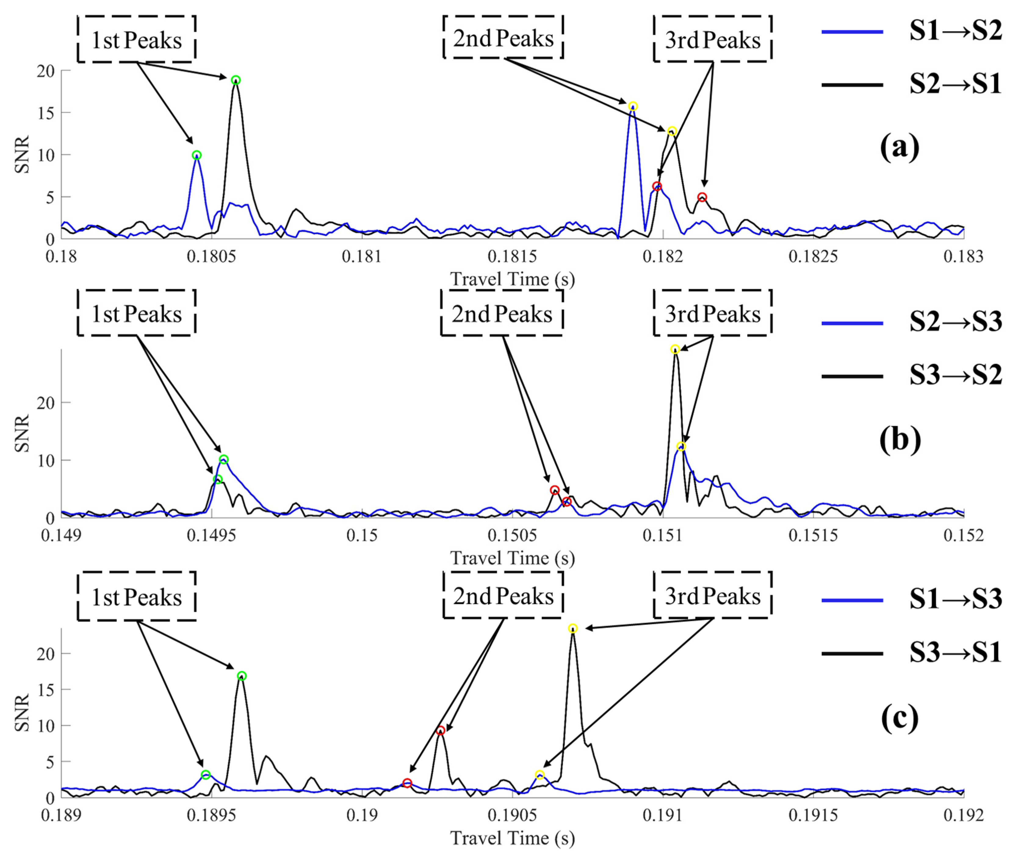
Figure 7.
Peak identification of acoustic signal propagated between sound station pairs at a particular time. (a–c) The sound propagation path results of S1–S2, S2–S3 and S3–S1, respectively.
Figure 7.
Peak identification of acoustic signal propagated between sound station pairs at a particular time. (a–c) The sound propagation path results of S1–S2, S2–S3 and S3–S1, respectively.
Figure 8.
Multi-peaks identification. (a–c) The results of peak extraction after S1–S2, S2–S3, and S3–S1 correlation, respectively. The abscissa axis in colormaps is the travel time of signals; the ordinate axis indicates the time at which signals were sent; the color depth value indicates the SNR. The magnified figures are shown as three-dimensional coordinates. The abscissa and ordinate coordinates are the same as the colormap, and the height is the SNR value.
Figure 9.
Travel time deviations. (a–c) The travel time deviations of three peaks between S1–S2, S2–S3, and S3–S1, respectively.
Figure 9.
Travel time deviations. (a–c) The travel time deviations of three peaks between S1–S2, S2–S3, and S3–S1, respectively.
Figure 10.
Layer-averaged water temperature between three sound stations. (a–c) The temperature inversion results of vertical slices between stations (red lines indicate the temperature of each layer (7.5 m, 20 m, 28 m), blue lines indicate the results passing through the 1 h weighted moving average). (d–f) Inversion errors (the red, black, blue lines indicate the first, second, and third layers, respectively.).
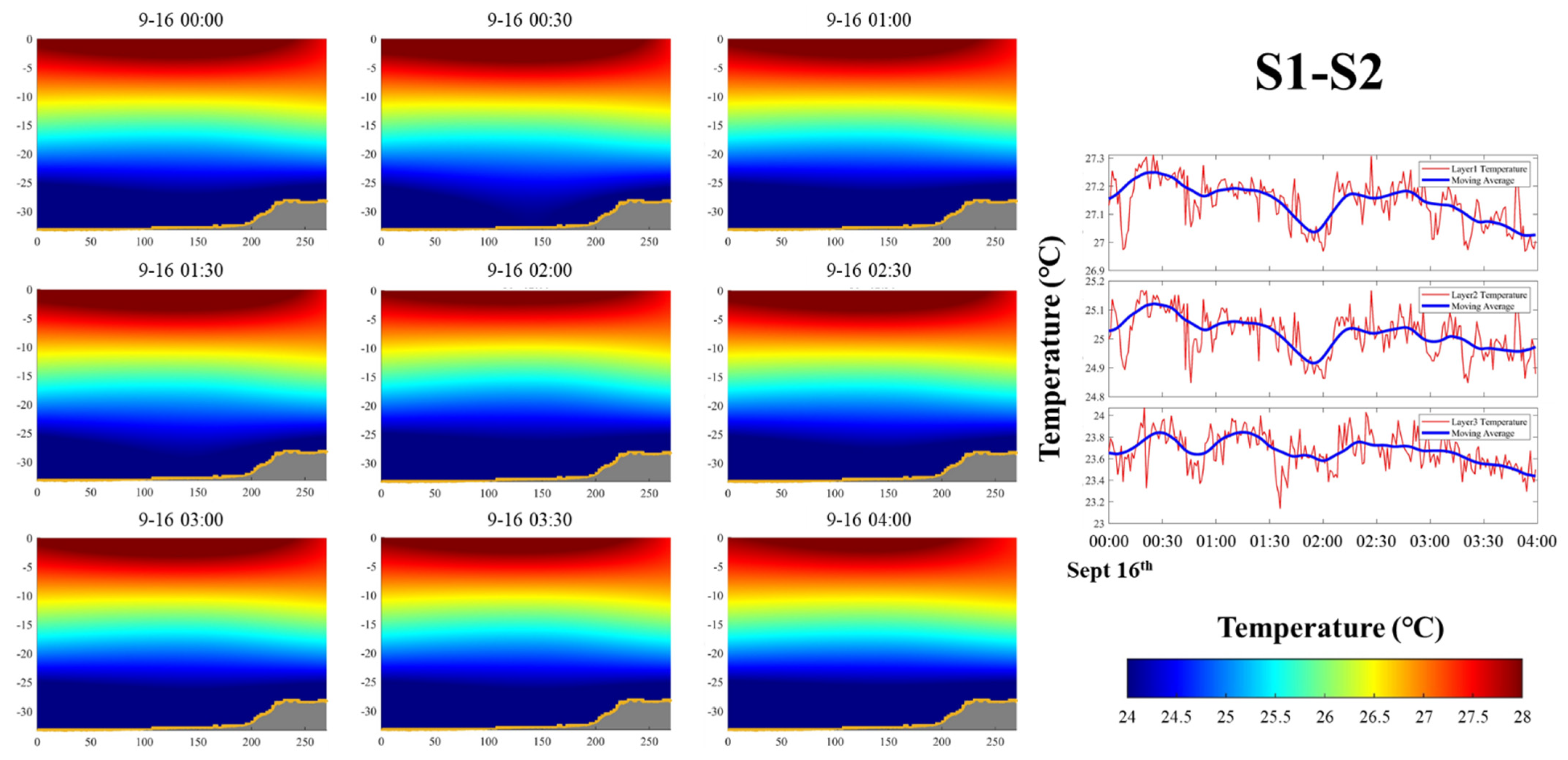
Figure 11.
Colormaps of the water temperature field along a vertical slice between stations S1 and S2. The figure on the right shows the temperature of each layer in the corresponding time period intercepted from
Figure 10.
Figure 11.
Colormaps of the water temperature field along a vertical slice between stations S1 and S2. The figure on the right shows the temperature of each layer in the corresponding time period intercepted from
Figure 10.
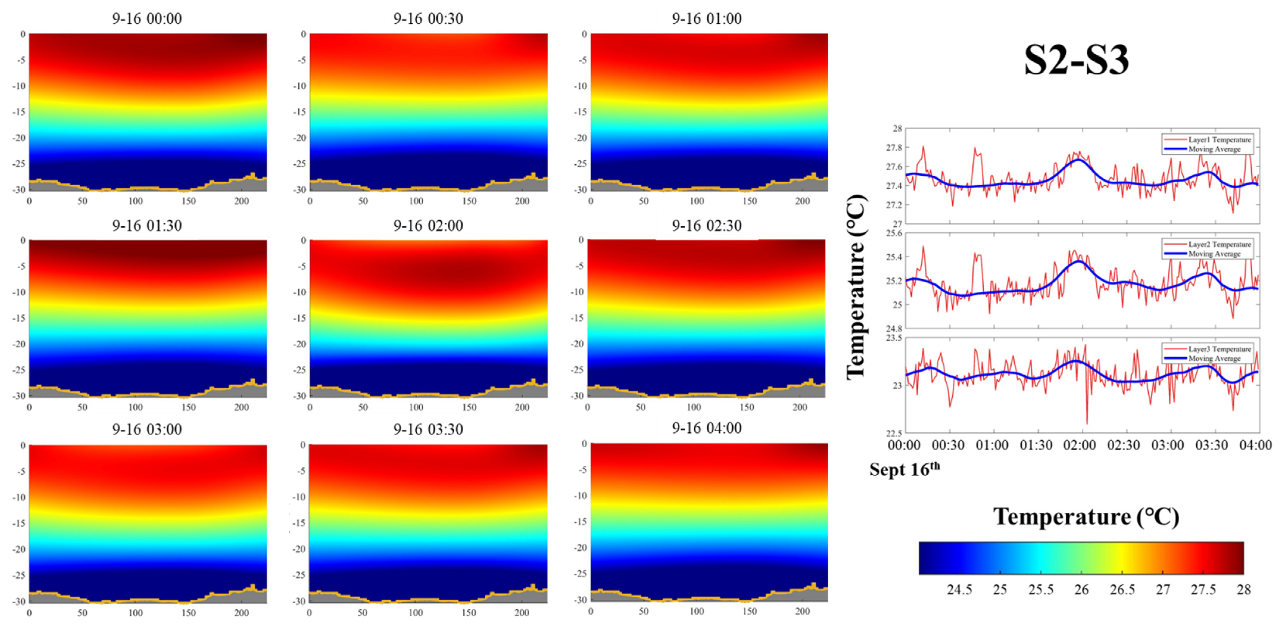
Figure 12.
Colormap of the vertical temperature field between stations S2 and S3. The figure on the right shows the temperatures of each layer in the corresponding time period intercepted from
Figure 10.
Figure 12.
Colormap of the vertical temperature field between stations S2 and S3. The figure on the right shows the temperatures of each layer in the corresponding time period intercepted from
Figure 10.
Figure 13.
Colormap of the vertical temperature field between stations S3 and S1. The figure on the right shows the temperatures of each layer in the corresponding time period intercepted from
Figure 10.
Figure 13.
Colormap of the vertical temperature field between stations S3 and S1. The figure on the right shows the temperatures of each layer in the corresponding time period intercepted from
Figure 10.
Figure 14.
Comparison of layer average water temperature. (a–c) The comparison of average temperature curves between the grid method and the layer-averaged method. The red and blue lines indicate the average temperature in each layer obtained by the grid method and the layer-averaged method after a weighted moving average.
Table 1.
Acoustic signal and sound station parameters.
Table 1.
Acoustic signal and sound station parameters.
| Item | Value |
|---|
| Central frequency (kHz) | 50 |
| Order of M sequence | 10 |
| Q 1 | 2 |
| Transmit interval (min) | 1 |
| Start and end date | Sept.15 09:00–Sept.16 16:00 |
| Station | S1 | S2 | S3 |
| Station distance (m) 2 | L12 = 270.00 | L23 = 224.01 | L31 = 283.64 |
| Transceiver depth (m) | 20 | 20 | 16.86 |
Table 2.
Ray length in each layer and reference travel time (three rays and three layers).
Table 2.
Ray length in each layer and reference travel time (three rays and three layers).
| Stations | S1–S2 | S2–S3 | S3–S1 |
|---|
| Ray Path | D 1 | S 2 | B 3 | D | S | B | D | S | B |
|---|
| Layer 1 | 0 | 209.946 | 0 | 0 | 188.490 | 0 | 0 | 238.576 | 0 |
| Layer 2 | 270.068 4 | 272.983 | 142.737 | 224.037 | 38.509 | 139.634 | 283.775 | 47.533 | 249.815 |
| Layer 3 | 0 | 0 | 129.167 | 0 | 0 | 85.523 | 0 | 0 | 34.515 |
| Total 4 (m) | 270.068 | 272.98 | 271.904 | 224.037 | 226.999 | 225.157 | 283.775 | 286.109 | 284.33 |
| TT 5 (s) | 0.18038 | 0.18191 | 0.18217 | 0.14962 | 0.15124 | 0.15061 | 0.18947 | 0.19061 | 0.19010 |
Table 3.
Ray length in each grid and reference travel time (three rays and nine grids).
Table 3.
Ray length in each grid and reference travel time (three rays and nine grids).
| Stations | S1–S2 | S2–S3 | S3–S1 |
|---|
| Ray Path | D | S | B | D | S | B | D | S | B |
|---|
| Grid 1 | 0 | 70.033 | 0 | 0 | 42.469 | 0 | 0 | 66.249 | 0 |
| Grid 2 | 0 | 100.97 | 0 | 0 | 101.22 | 0 | 0 | 100.73 | 0 |
| Grid 3 | 0 | 38.944 | 0 | 0 | 44.802 | 0 | 0 | 28.498 | 0 |
| Grid 4 | 100.03 | 31.114 | 26.504 | 70.027 | 28.55 | 58.125 | 100.01 | 34.605 | 59.162 |
| Grid 5 | 100.01 | 0 | 46.182 | 100.01 | 0 | 27.246 | 100.01 | 0 | 45.837 |
| Grid 6 | 70.028 | 31.924 | 70.05 | 54 | 9.958 | 54.262 | 83.755 | 56.027 | 83.712 |
| Grid 7 | 0 | 0 | 75.167 | 0 | 0 | 12.147 | 0 | 0 | 44.367 |
| Grid 8 | 0 | 0 | 54.001 | 0 | 0 | 73.377 | 0 | 0 | 54.252 |
| Grid 9 | 0 | 0 | 0 | 0 | 0 | 0 | 0 | 0 | 0 |
| Total (m) | 270.068 | 272.98 | 271.904 | 224.037 | 226.999 | 225.157 | 283.775 | 286.109 | 284.33 |
| TT (s) | 0.18038 | 0.18191 | 0.18217 | 0.14962 | 0.15124 | 0.15061 | 0.18947 | 0.19061 | 0.19010 |
Table 4.
The arrival time of each peak between sound stations (unit: s).
Table 4.
The arrival time of each peak between sound stations (unit: s).
| Peaks | S1→S2 | S2→S1 | S12-RS 1 |
| 1st Peak | 0.1804 | 0.1805 | 0.18038 | D |
| 2nd Peak | 0.1819 | 0.1820 | 0.18191 | S |
| 3rd Peak | 0.1820 | 0.2821 | 0.18217 | B |
| Peaks | S2→S3 | S3→S2 | S23-RS |
| 1st Peak | 0.1495 | 0.1496 | 0.14962 | D |
| 2nd Peak | 0.1506 | 0.1507 | 0.15061 | B |
| 3rd Peak | 0.1510 | 0.1511 | 0.15124 | S |
| Peaks | S1→S3 | S3→S1 | S13-RS |
| 1st Peak | 0.1895 | 0.1896 | 0.18947 | D |
| 2nd Peak | 0.1902 | 0.1903 | 0.19010 | B |
| 3rd Peak | 0.1906 | 0.1907 | 0.19061 | S |
Table 5.
Mean and standard deviation of travel time deviations.
Table 5.
Mean and standard deviation of travel time deviations.
| Stations | S1–S2 | S2–S3 | S3–S1 |
|---|
| Peaks | 1st Peak | 2nd Peak | 3rd Peak | 1st Peak | 2nd Peak | 3rd Peak | 1st Peak | 2nd Peak | 3rd Peak |
|---|
| Terr-M 1 | 0.0097 | 0.0164 | 0.0496 | 0.0019 | 0.0114 | 0.0652 | 0.0037 | 0.0114 | 0.1677 |
| Terr-S 2 | 0.0013 | 0.0005 | 0.0008 | 0.0013 | 0.0142 | 0.1677 | 0.0031 | 0.0026 | 0.0456 |
Table 6.
RMSEs of the comparison of the average water temperature in each layer obtained by the grid method and the layer-averaged method.
Table 6.
RMSEs of the comparison of the average water temperature in each layer obtained by the grid method and the layer-averaged method.
| RMSE (°C) 1 | S1–S2 | S2–S3 | S3–S1 |
|---|
| Layer 1 | 0.0122 | 0.0359 | 0.0073 |
| Layer 2 | 0.0042 | 0.0084 | 0.0082 |
| Layer 3 | 0.0963 | 0.0873 | 0.0712 |


