Article

Integrating Phenological and Geographical Information with Artificial Intelligence Algorithm to Map Rubber Plantations in Xishuangbanna

1
Centre for Mountain Futures (CMF), Kunming Institute of Botany, Kunming 650201, China
2
Key Laboratory for Economic Plants and Biotechnology, Kunming Institute of Botany, Chinese Academy of Sciences, Kunming 650201, China
3
University of Chinese Academy of Sciences, Beijing 100049, China
4
East and Central Asia Regional Office, World Agroforestry (ICRAF), Kunming 650201, China
*
Author to whom correspondence should be addressed.
Remote Sens. 2021, 13(14), 2793; https://0-doi-org.brum.beds.ac.uk/10.3390/rs13142793
Submission received: 30 May 2021 / Revised: 8 July 2021 / Accepted: 13 July 2021 / Published: 16 July 2021

Abstract

:
Most natural rubber trees (Hevea brasiliensis) are grown on plantations, making rubber an important industrial crop. Rubber plantations are also an important source of household income for over 20 million people. The accurate mapping of rubber plantations is important for both local governments and the global market. Remote sensing has been a widely used approach for mapping rubber plantations, typically using optical remote sensing data obtained at the regional scale. Improving the efficiency and accuracy of rubber plantation maps has become a research hotspot in rubber-related literature. To improve the classification efficiency, researchers have combined the phenology, geography, and texture of rubber trees with spectral information. Among these, there are three main classifiers: maximum likelihood, QUEST decision tree, and random forest methods. However, until now, no comparative studies have been conducted for the above three classifiers. Therefore, in this study, we evaluated the mapping accuracy based on these three classifiers, using four kinds of data input: Landsat spectral information, phenology–Landsat spectral information, topography–Landsat spectral information, and phenology–topography–Landsat spectral information. We found that the random forest method had the highest mapping accuracy when compared with the maximum likelihood and QUEST decision tree methods. We also found that adding either phenology or topography could improve the mapping accuracy for rubber plantations. When either phenology or topography were added as parameters within the random forest method, the kappa coefficient increased by 5.5% and 6.2%, respectively, compared to the kappa coefficient for the baseline Landsat spectral band data input. The highest accuracy was obtained from the addition of both phenology–topography–Landsat spectral bands to the random forest method, achieving a kappa coefficient of 97%. We therefore mapped rubber plantations in Xishuangbanna using the random forest method, with the addition of phenology and topography information from 1990–2020. Our results demonstrated the usefulness of integrating phenology and topography for mapping rubber plantations. The machine learning approach showed great potential for accurate regional mapping, particularly by incorporating plant habitat and ecological information. We found that during 1990–2020, the total area of rubber plantations had expanded to over three times their former area, while natural forests had lost 17.2% of their former area.

1. Introduction

The para rubber tree (Hevea brasiliensis) is the major source of natural rubber for global industrial markets, producing more than 98% of the world’s natural rubber [1,2]. With growing demand for natural rubber, led mainly by the tire industry, rubber plantations are now widely planted outside their historically planted zone (between 10°N and 10°S latitude), to areas as far as 22°N, including Hainan and Yunnan of China and other regions of southeast Asia [1,3,4,5]. Plantations are projected to expand by 4.3~8.5 million ha within a decade [3]. The expansion of rubber plantations has negative consequences for local biodiversity, carbon stocks, the water cycle, and other ecosystem services, especially for those at higher elevations and with steeper slopes [6,7]. Knowing the spatial distribution of rubber plantation areas at a relatively high resolution (30 m or finer), with a high degree of accuracy, is thus of great importance to regional planning, sustainable rubber development in the global industry market, and global biogeochemical processes in the carbon and water cycles [4,8]. Mapping with a high accuracy at a high resolution is the basis for land use planning, mapping productivity, carbon finance schemes, conservation policies, and the assessment of economic losses caused by diseases (e.g., powdery mildew disease) or natural disasters (e.g., typhoons). Therefore, using remote sensing to map rubber plantations can play an important role for rubber markets at both local and global scales, land use planning, and economic loss assessment.
Satellite remote sensing has become the main approach for large-scale rubber plantation mapping, especially since the United States Geological Survey’s (USGS) Landsat time series data became freely available in 2008 [9,10]. Landsat time series data were then widely used in local and global land use/land cover mapping [11,12]. Compared to previous classification schemes that were based on spectral pixel or texture features, biophysical and physical features of rubber trees have been widely used to improve the efficiency and accuracy of rubber plantation mapping during recent years [12,13,14]. Studies have mapped rubber plantations using the Moderate Resolution Imaging Spectroradiometer (MODIS) by adding deciduous feature-based phenological information in order to improve classification [15,16,17]. However, the 250 m resolution MODIS is relatively coarse, making it difficult to map rubber plantations accurately in fragmented landscapes, and there is uncertainty regarding its accuracy for areas with mixed land cover [18]. Researchers have also used Landsat time series data to achieve accurate and finer mappings of rubber plantations by adding Landsat-derived vegetation indices, which track well at the phenology of deciduous rubber plantations [12,14,19,20,21]. However, the complex and fragmented landscape of Xishuangbanna means the accuracy of such models is uncertain. This is further complicated by the mix of other land use types (e.g., paddy rice). Therefore, in later research, Xiao and colleagues (2020) added a digital elevation model (DEM) layer in order to improve the accuracy [22,23]. We found a few previous studies that had included DEM among the classifiers, which demonstrated the great potential of DEM to improve the efficiency and accuracy of rubber plantation mapping, especially for rugged regions [22,23,24].
To date, multiple classification approaches have been used in mapping rubber plantations by combining phenological information, among which the maximum likelihood (ML) classification method, QUEST decision tree (QDT) classification method [12,18,25], object-based classification method [15,20], the random forest method (RF) [17,26], and other machine learning-based classification methods [26] have been widely used. However, limited information exists on how these classifiers perform when phenological information is incorporated.
In this paper, we will assess the application of the above three classifiers (maximum likelihood classification, QUEST decision tree, and random forest) to phenological based/topographical-based rubber plantation mapping. We address three objectives: (1) to assess the accuracy and stability of three classifiers based on four data inputs for mapping rubber plantations; (2) to assess the performance of phenological and topographical information for mapping rubber plantations; and (3) to update rubber plantation distribution maps for Xishuangbanna.

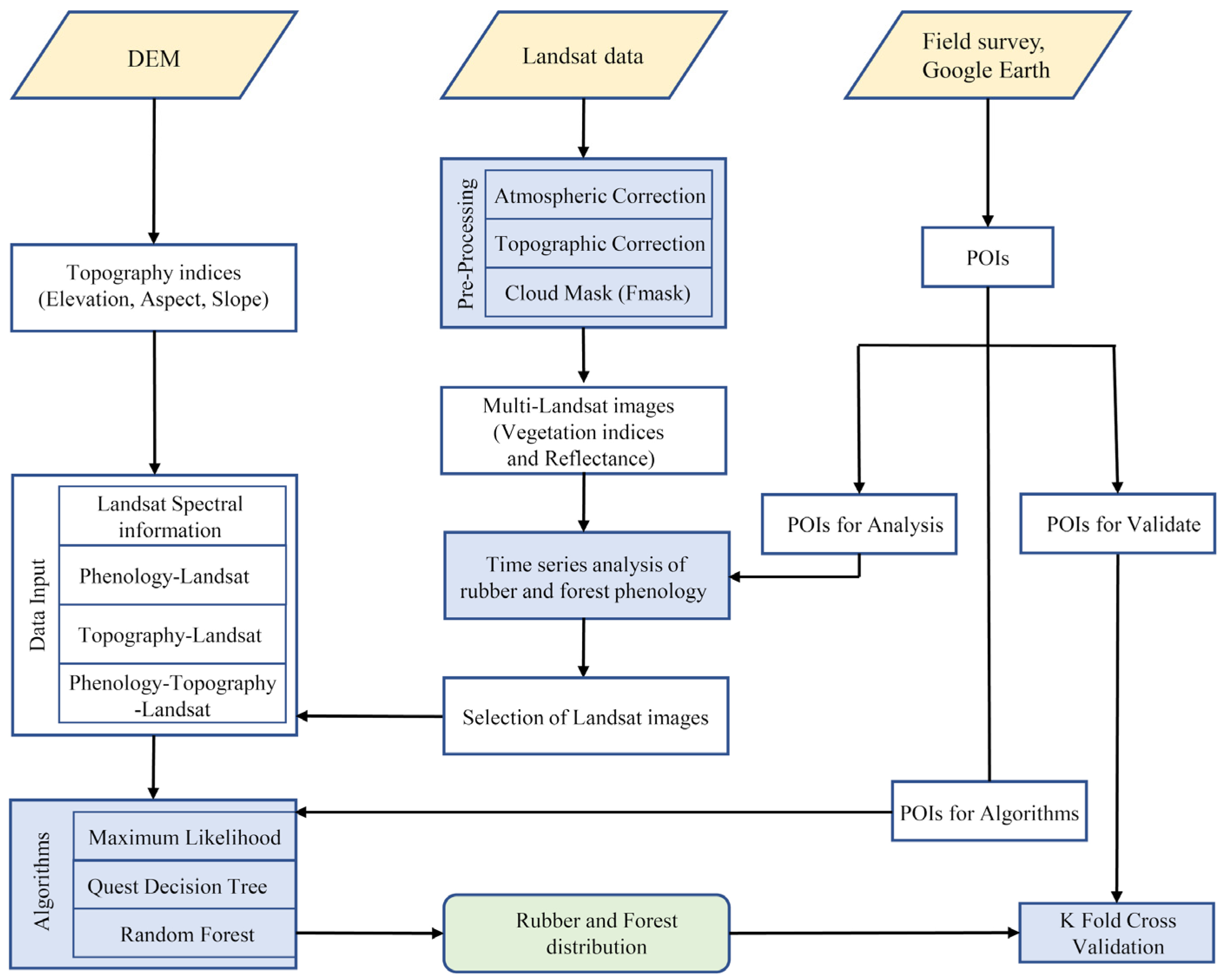
2. Materials and Methods
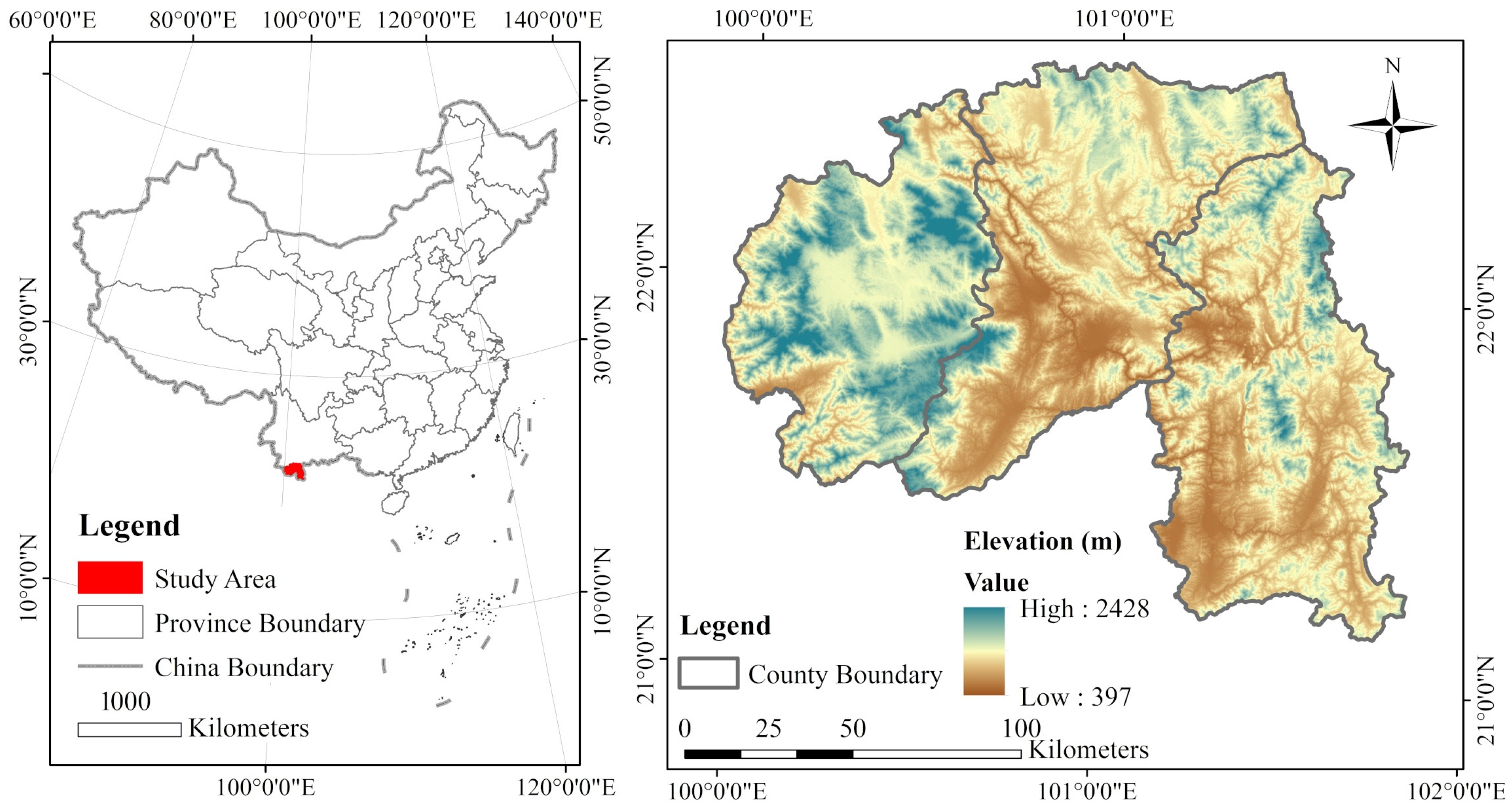
2.1. Study Area

Xishuangbanna is the second largest natural rubber development region in China. It is located at the northern edge of the Asian tropical zone (Figure 1) [27,28]. Compared to the flat landscape of the largest rubber producing region of Hainan, Xishuangbanna is much more mountainous, with elevations ranging from 397 m to 2428 m. Around 35.9% of the land is above 1200 m, and only 18.1% below 800 m. Xishuangbanna has a tropical monsoon climate with two seasons: the rainy season (May–October) and the dry season (November–April), which is further divided into a cool-dry season (November–February) and a hot-dry season (March–April) [29,30]. The cool-dry season features the lowest annual temperatures and little rainfall. The annual average temperature of Xishuangbanna is 22.6 °C, and annual average rainfall is 1130 mm, with more than 80% of the rainfall occurring in the rainy season [31].
In contrast to the natural evergreen forests of Xishuangbanna, rubber trees experience interannual leaf defoliation (or ‘wintering’, from early December to the middle of January) and refoliation (from the end of January to the end of March) [31]. This interannual defoliation (via leaf shedding or wintering) and foliation (emergence of new leaves or leaf flushing) of rubber trees provides a physiological and phenological basis by which remote sensing techniques can be used to distinguish between rubber plantations and natural forest. However, we found that variation in the timing of defoliation and refoliation, which are affected by climate, rubber clones, and locations [31,32], might affect the temporal window for selecting candidate images. The growth of rubber trees requires relatively high temperatures and precipitation. Even for cold-tolerant clones, rubber trees are unproductive at higher and steeper areas [7]. Therefore, the distribution of rubber trees in Xishuangbanna is significantly affected by topographical factors [7,24].

2.2. Landsat Images and Data Pre-Processing

We used Level 1 terrain-corrected standard surface reflectance products of the Landsat time series data of the United States Geological Survey (USGS) Earth Resources Observation and Science (EROS) Center Science Processing Architecture (ESPA). We freely downloaded the data from the geospatial data cloud (http://www.gscloud.cn/, accessed on 25 December 2020) (Table 1). Landsat images from 1989 to 2011 are Thematic Mapper sensor (TM) and images from 2018 to 2020 are Operational Land Imager (OLI). The Level 1 terrain-corrected products have consistent geometric, radiometric, and precision corrections, and are also inter-calibrated across different Landsat sensors.
The pre-processing of the Landsat time series images included a quality check, atmosphere correction, and topographic rectification. Atmospheric correction of the surface reflectance data was generated from the Landsat Ecosystem Disturbance Adaptive Processing System (LEDAPS), and we further corrected the data with Fast Line-of-sight Atmospheric Analysis of Spectral Hypercubes (FLAASH). The Landsat images were then processed for topographic rectification using the Teillet model, and we used Global Digital Elevation Model Version 2 (GDEM V2) for the model. GDEM V2 was downloaded from the geospatial data cloud (http://www.gscloud.cn/, accessed on 28 December 2020) and processed in ArcGIS 10.3. The Fmask model has been used to filter pixels caused by clouds and identify shadows. The workflow is shown in Figure 2.
For the candidate Landsat images, we calculated the Normalized Difference Vegetation Index (NDVI) [33], Enhanced Vegetation Index (EVI) [34], and Land Surface Water Index (LSWI) [35]:
NDVI = ρ n i r ρ r e d ρ n i r + ρ r e d
EVI = 2.5 × ρ n i r ρ r e d ρ n i r + 6 × ρ r e d 7.5 × ρ b l u e + 1  
LSWI = ρ n i r ρ s w i r 1 ρ n i r + ρ s w i r 1  
where   ρ b l u e ,   ρ r e d ,   ρ n i r , and ρ s w i r 1 are the reflectance values of blue band, red band, near-infrared band (NIR), and shortwave-infrared band (SWIR) in Landsat images, respectively. Regarding EVI, the canopy background adjustment factor is 1, and the aerosol resistance weights are 6 and 7.5.

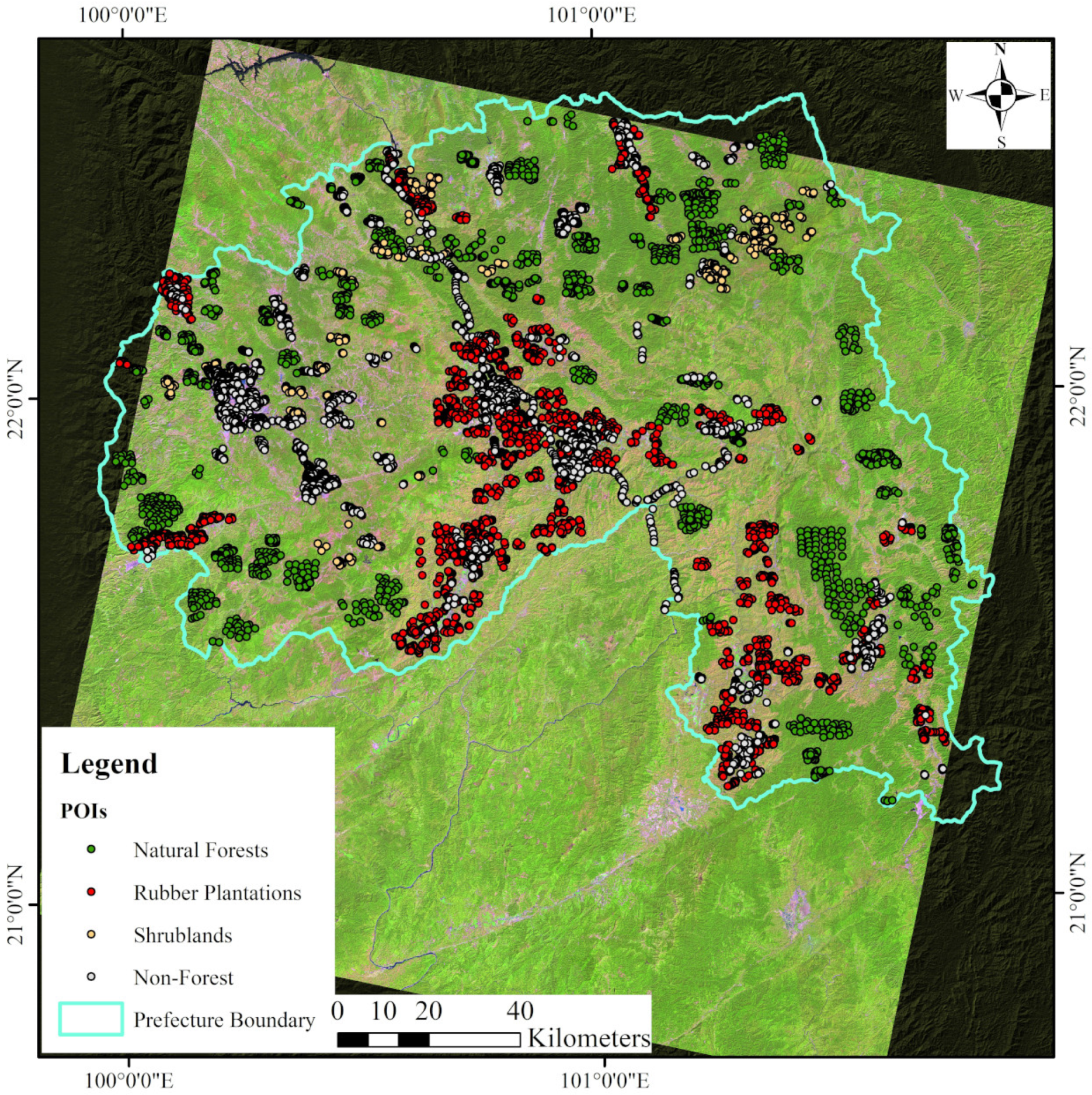
2.3. Ground Reference Data

We collected ground-truth data for 2020 using stratified sampling based on a thematic map from 2014 [36]. In January 2021, we conducted a field survey in Xishuangbanna in order to collect ground-truthing data, which were then double-checked on Google Earth. Finally, 3546 points of interests (POIs) were collected (Figure A1), which included 827 points for natural forests, 611 for rubber plantations, 218 for shrublands, 211 for water bodies, 319 for constructed lands, 1199 for cultivated lands, and 161 for tea plantations. For the natural forests, we collected the points along different slopes, aspects, and even valleys to cover all the forest types. The rubber plantations included both young and mature plantations. The water bodies included rivers, reservoirs, and lakes. The cultivated lands included paddy fields, non-irrigated farmland, and banana plantations. The constructed lands included both urban and rural settlements, mining sites, and roads. We then randomly collected 5946 POIs on Google Earth (Figure A1), with the aim to cover the whole of Xishuangbanna. Among these POIs, there were 2481, 1833, 654, 257, 189, 452, and 80 POIs for natural forests, rubber plantations, shrublands, water bodies, constructed lands, cultivated lands, and tea plantations, respectively. We classified water bodies, constructed lands, cultivated land, and tea plantations as non-forests. We used 460 and 780 points of ground-truthing data from Chen et al. (2016) and Yi et al. (2013) for the years of 1990 and 2000 [6,7], and 1462 from Chen et al. (2016) and Zhai et al. (2018) for the year of 2010 [6,20]. In addition, we used Google Earth and Landsat images to randomly select 9048, 7936, and 8906 POIs from 1990, 2000, and 2010, respectively.

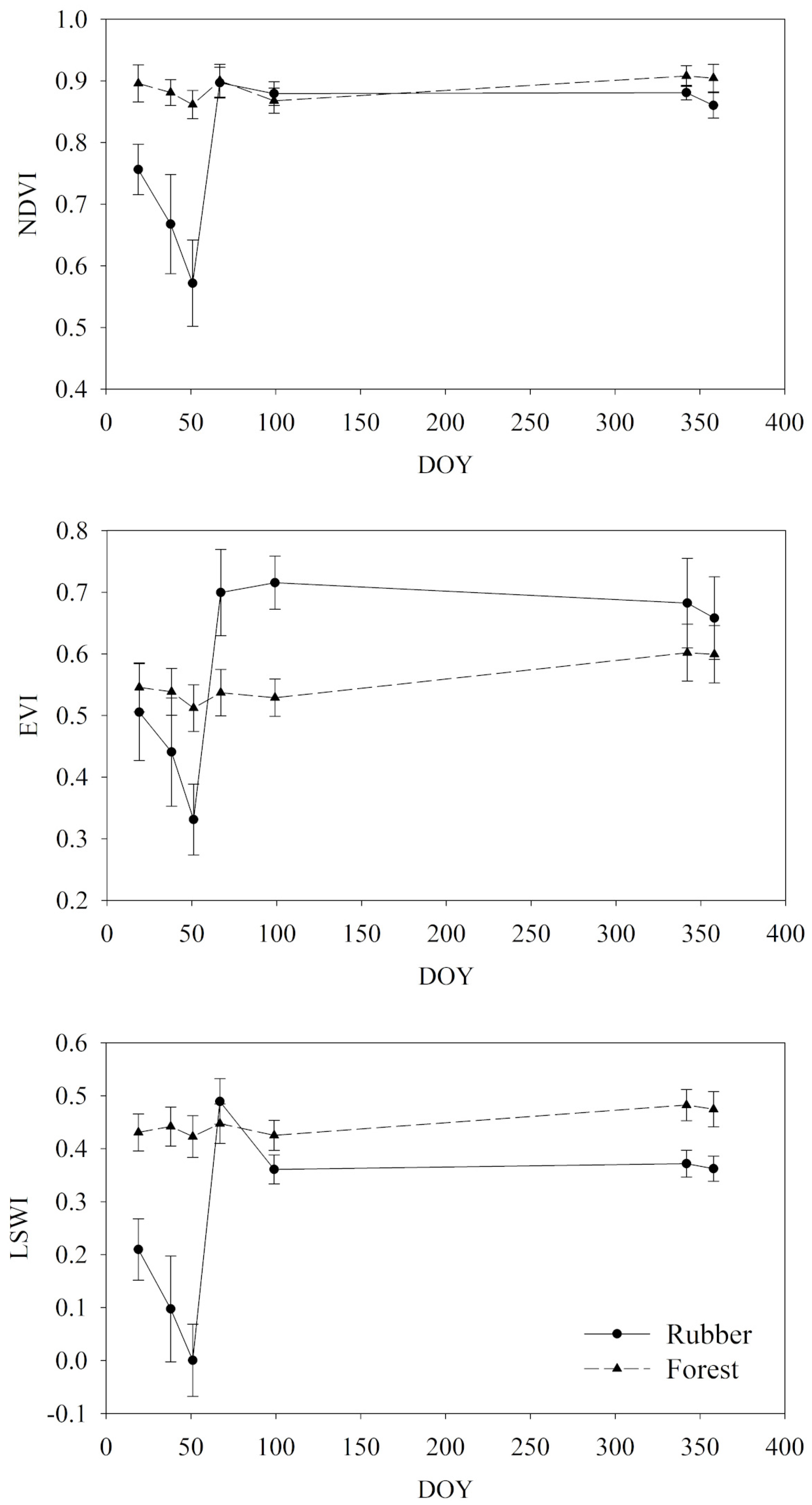
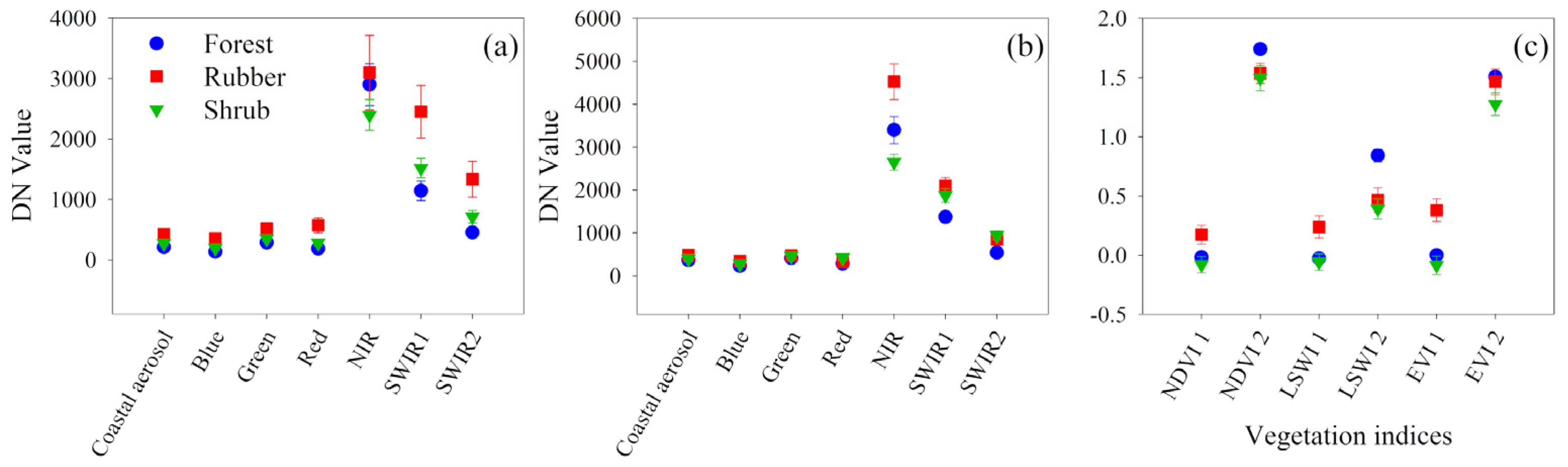
2.4. Seasonal Changes and Spectral Features of Rubber Plantations and Natural Forests

Although previous studies have investigated the seasonal changes in rubber plantations [12,14,20], we checked these using the most recent Landsat OLI images from 2018–2019. Seven images at the Path/Row of 130/45 were finally selected to investigate seasonal changes. The date of year (DOY) and year were 19 (2018), 38 (2019), 51 (2018), 67 (2018), 99 (2018), 342 (2019), and 358 (2019), respectively. All of the images used to capture the seasonal changes were freely downloaded from the geospatial data cloud (http://www.gscloud.cn/, accessed on 4 January 2021). All of these images underwent FLAASH-based atmospheric correction and Teillet model-based topographic correction. The NDVI, EVI, and LSWI of each Landsat OLI image was calculated. We then derived the NDVI, EVI, and LSWI of rubber plantations and natural forests using fifty rubber plantation points from state farms and fifty natural forest points from nature reserves from Google Earth. Another fifty points of shrublands were selected to check the spectral differences with natural forests and rubber plantations.

2.5. Classification Algorithm

In this study, we used the ML, QDT, and RF to investigate mapping efficiency and accuracy for Xishuangbanna.
Rubber plantations in Xishuangbanna underwent defoliation and refoliation from December to March of the following year, which was captured by the Landsat images (Figure 3). Rubber plantations experienced defoliation from early January to the end of February before undergoing a refoliation period from early March to the middle of April (Figure 3). Previous studies had found that phenological spectral information or vegetation indices-based phenological information in rubber defoliation and refoliation periods can effectively identify rubber plantations and other vegetation [12,20,22]. Therefore, the spectral differences between rubber refoliation and defoliation of the three vegetation indexes EVI, NDVI, and LSWI were used to capture changes in rubber phenology, which were calculated in the ENVI 5.3, e.g., E V I r e f o l i a t e E V I d e f o l i a t e and E V I r e f o l i a t e + E V I d e f o l i a t e , and the same was carried out for NDVI and LSWI.
Topography is a limiting factor for rubber expansion in Xishuangbanna, and it was found that rubber trees are mainly planted below 1200 m [6,37]. Therefore, this study calculated the topography indexes, including elevations, slopes, and aspects, in order to assess topographical influences on rubber mapping.
Accordingly, our spectral bands were classified into three groups: Landsat spectral band information (7 non-thermal bands: coastal aerosol, blue, green, red, NIR, SWIR1, and SWIR2), vegetation indices derived from phenological information (EVI, NDVI, and LSWI), and topographic indices (elevation, slope, and aspect). To investigate the performance of the three classification methods and the input information of spectral, phenology, and topography, four kinds of input data have been assessed for each classification: bands of Landsat images, phenology information (e.g., E V I r e f o l i a t e     E V I d e f o l i a t e and E V I r e f o l i a t e + E V I d e f o l i a t e for EVI), topographic indices, and phenology and topography information (combined phenology and topographic indices), which finally produced twelve outcomes. We recorded input data for the classification of Landsat spectral bands (L), phenology–Landsat spectral bands (PL), topography–Landsat spectral bands (TL), and phenology–topography–Landsat spectral bands (PTL). For clarity, we recorded each according to the input data and the classification approach, e.g., the images classified by the RF algorithm with the input information of PL would be recorded as PL–RF classification. We ran all classifications in the ENVI environment.

2.6. Rubber Plantation Mapping in Xishuangbanna during 1990–2020

It was found the PTL-based RF algorithms achieved the highest accuracy in 2020 as well as the lowest commission and omission. Therefore, PTL-based RF algorithms were employed to map the rubber plantations of Xishuangbanna in 1990, 2000, and 2010. Finally, we mapped rubber plantations from 1990–2020 and updated them for 2020.

2.7. Validation and Comparison

Cross-validation is an effective way to assess mapping results and algorithms for remote sensing [38]. We used K-fold cross validation of a randomly selected subset of 80% of POIs as training sets for mapping the land use/land cover in Xishuangbanna in 2020. The remaining 20% of POIs were used to assess the produced map [38]. In order to reduce overfitting, we repeated these steps 10 times, for both training and accuracy assessment for each classifier (Figure 5). We then employed the F1 Score (FS) to assess the mapping accuracy [39]. The mean value (MV) and standard deviation (SD) of the FS and kappa coefficient (KA) were used to assess the mapping accuracy and stability of the classifiers (Figure 5). In addition, we also assessed the mapping accuracy of each classifier by the producer’s accuracy (PA), user’s accuracy (UA), and overall accuracy (OA) metrics (Table 2).

3. Results

3.1. The Phenological Characteristics of Rubber Plantations and Natural Forests

The vegetation indices had better separability than the seven Landsat bands, among which the SWIR1 performed better in separating the rubber from the natural forests than other Landsat bands (Figure 3 and Figure 4b). NDVI, LSWI, and SWIR1 performed better during both defoliation and refoliation than the Landsat bands (Figure 3 and Figure 4b). Further analysis of the NDVI, LSWI, and EVI between defoliation and refoliation found that rubber plantations could be separated from natural forests and shrublands, while it was difficult to separate natural forests from the shrublands (Figure 4c).

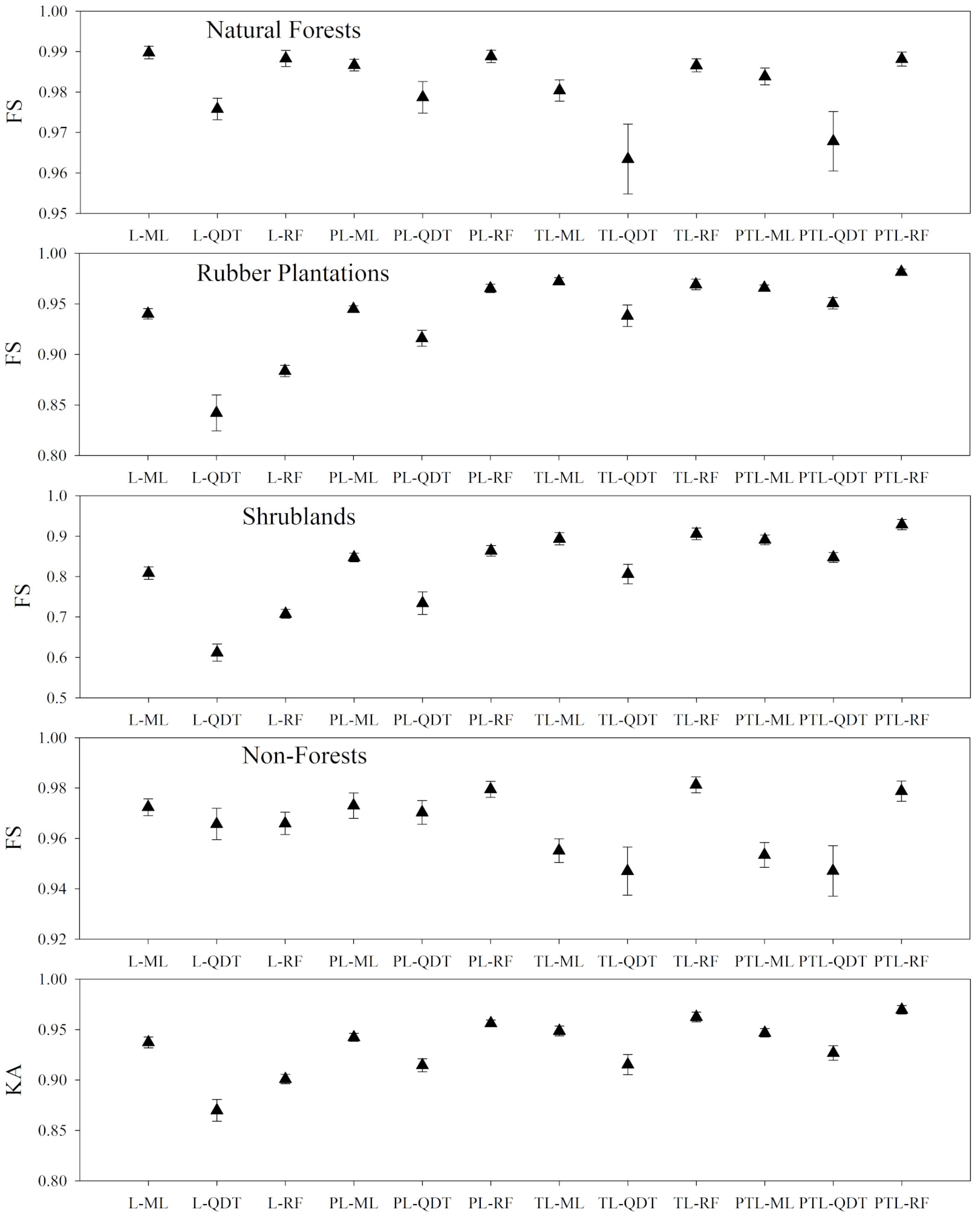
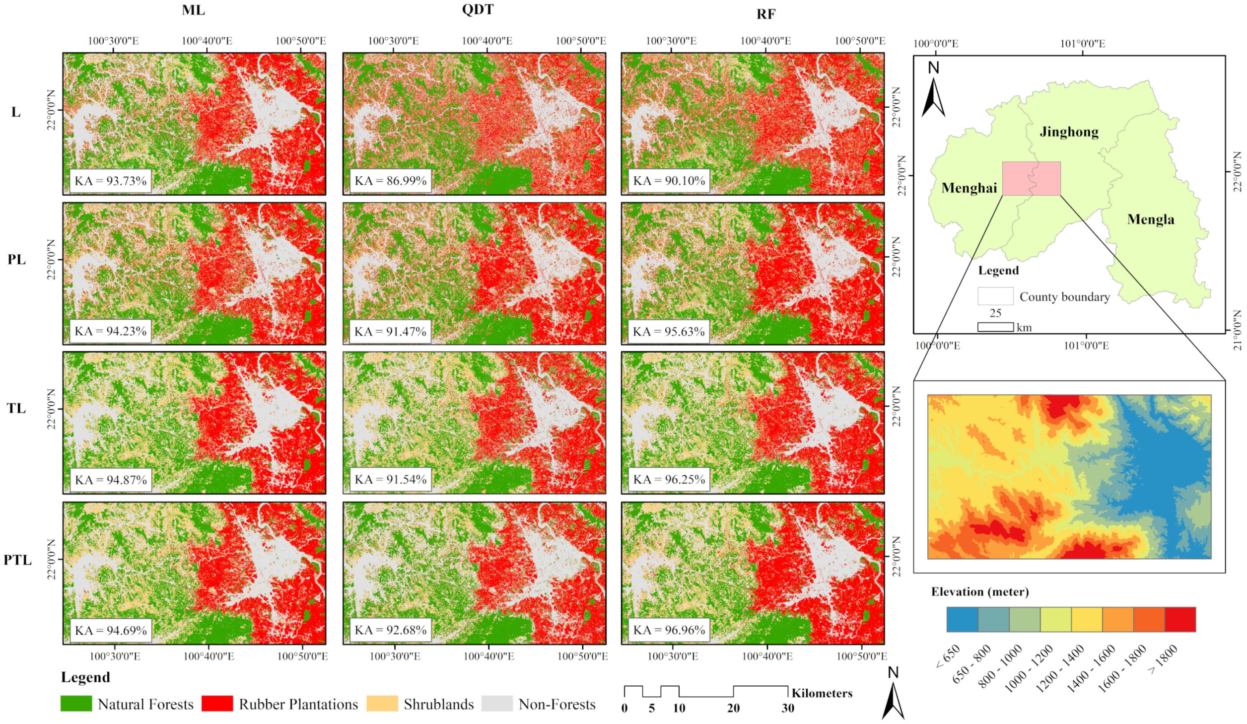
3.2. Random Forest Algorithm-Based Classifier Performs Better Than the Other Two Classifiers

We found that the RF classifier had the highest mapping accuracy compared to the ML and QDT classifiers.
For rubber plantation mapping, the highest user accuracy was classified by the RF classifier, followed by the ML and QDT classifiers for the classification of TL, PL, and PTL approaches. However, the ML classification performed better than the QDT and RF for the classification of L (Table 2 and Figure 5).
We further tested the three classifiers with four kinds of input information from Xishuangbanna (Figure 5 and Figure 6). The RF performed better than the other two classifiers. The PTL-based RF achieved the highest KA (Table 2). The QDT achieved higher KA when classified with PTL compared to the other three data input (L, TL, and PL) (Table 2 and Figure 5). However, the ML achieved higher KA when classified with TL. Without considering topography, rubber plantations were distributed across higher elevations using the RF classifier with L and PL compared to that with TL and PTL (Table 2, Figure 5 and Figure 6).

3.3. Either Phenology or Topography Could Improve Mapping Accuracy

We found that adding either phenological or topographical information to the classifiers could improve mapping accuracy (Table 2, Figure 5 and Figure 6). In particular, for topography, TL-based classification achieved higher accuracy than that of L and PL on both classifiers, while showing slightly lower accuracy than PTL-based RF and QDT classifiers. By adding topographical information, the TL-based classification improved KA by 3.95% and 0.45% over L and PL-based classification on all three classifiers, respectively (Table 2).
For rubber plantation mapping, the highest commission and omission error was produced by L with all three classifiers, which indicated that adding phenology and/or topography could decrease the commission and omission error (Table 2). Without the addition of phenology and/or topography, ML performed better than the other two classifiers, while by adding phenology, the RF classifier performed best with the lowest commission and omission error (2.36% and 4.54%, Table 2). By adding phenology, topography, or both, the QDT classifier performed worse than the other classifiers. The PTL had the lowest commission and omission error compared to the other three in all three classifiers, with the RF performing the best (97.53% and 98.80% for PA and UA). The above results indicated that either phenology or topography could improve rubber mapping accuracy, and both ML and RF could achieve reliable results (>92% for both PA and UA). In order to achieve higher mapping accuracy, it is recommended to use the RF classifier with the addition of phenology and topography; this combination is supported by its KA of 97%.

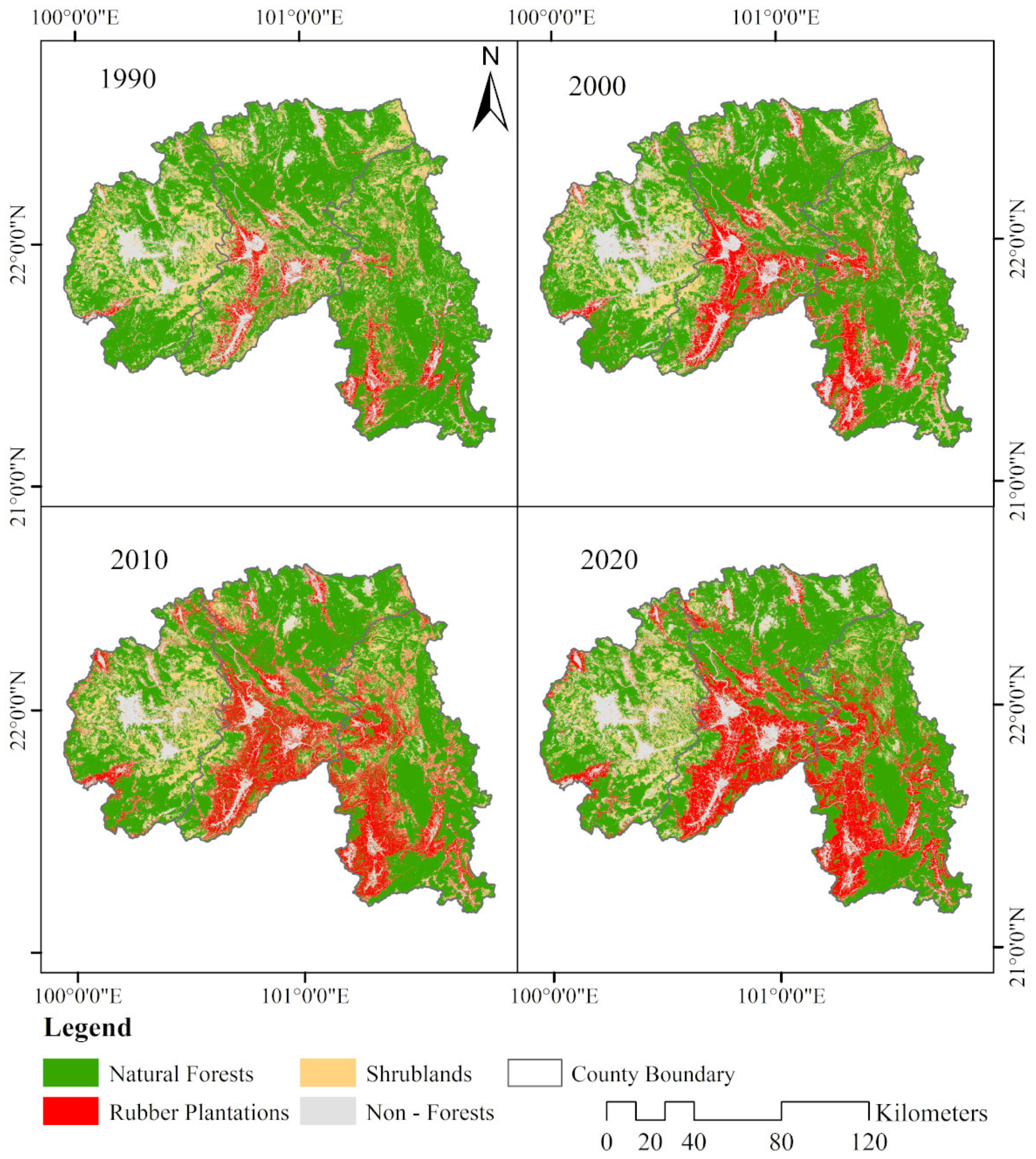
3.4. Natural Forests and Shrublands Were the Major Sources of the Increased Rubber Plantations

Between the years of 1990–2020, the area of rubber plantation more than tripled from 1.45 × 10³ km2 in 1990 to 4.46 × 10³ km2 in 2020, shifting from covering 7.58% of the area of the Xishuangbanna in 1990 to 23.24% in 2020 (Table 3 and Figure 7). Natural forests and shrublands were the two major sources for the new rubber lands, jointly contributing to 82.97% of the new rubber landcover (Table 4). Every ten years, 1.03 × 10³ km2 of natural forests and 0.56 × 10³ km2 of shrublands were converted to rubber plantations. From 1990–2020, more than 3.09 × 10³ km2 of natural forests were converted to rubber plantation, which occupies approximately 69.38% of the total rubber area by 2020, constituting 2.1 times the size of its area in 1990.
In contrast, from 1990–2020, Xishuangbanna lost 17.18% and 29.63% of its natural forests and shrublands, respectively. The degradation of natural forests to shrubland has markedly decreased, from 5.81% in 2000–2010 to 4.16% in 2010–2020, while during these two periods more shrublands have been reforested to natural forests, from 3.31% in 2000–2010 to 5.20% in 2010–2020, indicating that these degradation and reforestation patterns might be related to local conservation policies.

4. Discussion

In the current study, we used three classification approaches with four kinds of data input on Landsat imagery to investigate the mapping accuracy for rubber plantations. The results demonstrated that by adding phenology and topography information to the RF classifier, it has the potential for accurate mapping of mountainous and fragmented landscapes. Incorporating more data leads to higher accuracy when using the RF, indicating that RF could show a good performance while handling more input data, while minimizing overfitting.

4.1. Combining Phenological and Topographical Information to Improve the Mapping Efficiency for Rubber Plantations

Our results illustrate the benefits of using phenological information to improve rubber mapping accuracy [14,16,20,23,40]. The deciduous features of intra-annual defoliation and refoliation for rubber plantations differ from those of natural forests (Figure 3 and Figure 4). This distinction provides the basis for spectral discrimination between rubber plantations and other land uses [20,22]. The timing and duration of defoliation and refoliation periods varied between years, indicating that researchers need to check the phenological condition of the candidate images in advance [20,31,40]. Phenological information for rubber plantations is recommended for future mapping studies, especially for those based on artificial intelligence algorithms.
The inclusion of topography has also been found to improve rubber mapping accuracy, which might be related to the following three facts: (1) the growth and production of rubber plantations have a tropical climatic requirement for suitable temperature and precipitation. This shapes its distribution pattern both globally and within Xishuangbanna [3,41]; (2) the distribution of rubber plantations in Xishuangbanna is mainly across elevations below 1200 m a.s. [3,6,36,37,42]; and (3) rubber trees are an important industrial species, mainly planted in the form of monoculture in China, causing relatively homogeneous pixels in the relevant Landsat imagery [43]. However, the relatively better performance of RF, ML, and QDT with the topography input, compared to only the addition of phenology, indicated that machine learning or artificial intelligence approaches could use topography as an important assisting factor. Without considering topography, the object-based phenology approach in Zhang et al. (2019) might fail to distinguish between rubber plantations and seasonal deciduous tropical forests or shrublands in higher elevations [36,44] (Figure A2). We found that without topographical information, the classifier confounded rubber plantations with shrublands and natural forests, mostly failing to distinguish between rubber plantations and shrublands (Figure 5). It mainly overestimated the rubber plantation at the higher elevations, while underestimating it at the lower elevations (Figure A2). Therefore, as computing power improves, artificial intelligence algorithms should be developed that include the habits or habitat information of vegetation to the classifier in order to improve mapping accuracy. Xiao et al. (2020) used a DEM mask to facilitate rubber mapping efficiency in northern Laos after a decision-based forest cover extraction [22]. We found a high overestimation of rubber plantations on elevations higher than 1200 m using all the classifications besides topography (Figure A2). Therefore, phenological information could be used to improve mapping accuracy by combining with spectral bands. Combining topographical information with the classifier shows great potential in improving mapping accuracy for mountainous rubber-developing regions.

4.2. Random Forest Classifier Could Improve the Accuracy and Stability for Mapping Rubber Plantations

The stability and accuracy of RF were higher than that of QDT and ML algorithms for mapping rubber plantations, with a smaller SD (Figure 5). While comparing the SD, we found both the ML and RF had a smaller SD than the QDT classifier, which indicated that the QDT classifier had a lower stability and a lower accuracy, which was consistent with that of Xu et al. (2005) and Han et al. (2015) who found that the decision tree classifier not only may suffer from overfitting, but that its accuracy was also lower than that of RF [45,46]. A higher stability and accuracy were achieved by the RF based on the input data of PL, TL, and PTL. However, L-RF showed the lowest accuracy, which might relate to underfitting arising from the limited data inputs to the classifiers [47]. The higher stability of the RF may relate to the algorithm’s use of training data in order to develop trees, which was repeated more than 500 times in order to vote for each new datum input, with the most voted new datum input then produced for the final results [48,49,50]. The RF reduced overfitting and increased stability by the number of trees [51]. Due to the higher accuracy and stability of RF, we recommend using RF classifier-based phenological and topographical information for mapping rubber plantations.

4.3. Reversal of Rubber Plantations Expansion in Xishuangbanna

Using the PTL-based RF classifier, we mapped and updated the distribution of rubber plantations and natural forests until 2020. In 2020, rubber plantations occupied 23.2% of the area of Xishuangbanna, which was higher than the 22.4% in 2010 [6] while lower than that of 24.3% in 2014 [36] and slightly higher than that of 20.7% in 2018 [36]. It appears that rubber plantations achieved their highest coverage in Xishuangbanna in 2014, decreasing after 2014 until 2020 [36]. It is necessary to map the annual rubber plantation distribution after 2014 to investigate smallholder responses and behaviors, which are related to famer welfare and industrial safety and also have implications for the local plantation-related economy [52,53]. Our findings differed from the continuous expansion of rubber plantations previously reported for the region [54]. Smallholders might reduce their total rubber plantation area in the future, as low rubber latex prices continue to drop [53,55]. It appears that the continued expansion of rubber plantations is no longer a serious issue for local natural forest conservation, despite the strong global demand. With the continuous reduction of rubber prices starting in 2011 and the shrinking of its land area, the time for restoration work may be now, especially for steeper land and land with a higher elevation [56,57]. Our thematic maps provide the necessary support for future carbon storage calculations of rubber plantations in Xishuangbanna and for planning and implementing regional restoration projects.

5. Conclusions

In this study, we evaluated three widely used classification approaches for mapping rubber plantations, and we also evaluated four kinds of data inputs in order to investigate the mapping accuracy of phenology, topography, and Landsat-based spectral bands. We applied these three classification approaches with four kinds of data inputs across Xishuangbanna and further tested it in a small area (near the city of Jinghong) within Xishuangbanna. The RF achieved the highest producer and user accuracies, especially the RF classifier with PTL. This demonstrated the superior data processing abilities of artificial intelligence over statistical approaches. We also found that adding either phenology or topography could further improve the mapping accuracy, achieving higher producer and user accuracies than by only using L. We mapped the distribution of rubber plantations from 1990–2020 using the RF based on PTL. We found that from 1990–2020, the rubber plantations expanded while natural forests shrank. The land area occupied by rubber plantations more than tripled, whereas the natural forests lost more than 17% of their area. Natural forests and shrublands contributed to more than 80% of new rubber plantation cover, but it seems that this pattern of expansion did not continue after 2014. From 2014 onwards, the land area occupied by rubber plantations decreased. Our thematic maps provide necessary support for regional planning and ecosystem service assessments. The classification approach used in this study constitutes a trial of the effectiveness of combining artificial intelligence with growth habitat information for plants in order to improve mapping accuracy. Such an approach could also be used in other plantations and other ecosystems.

Author Contributions

Conceptualization, J.Y. and D.-L.Z.; methodology, J.Y. and D.-L.Z.; software, J.Y.; validation, J.Y. and D.-L.Z.; formal analysis, D.-L.Z.; investigation, J.Y. and D.-L.Z.; writing—original draft preparation, D.-L.Z.; writing—review and editing, D.-L.Z.; visualization, J.Y.; supervision, D.-L.Z. and J.X.; project administration, J.X.; funding acquisition, J.X. All authors have read and agreed to the published version of the manuscript.

Funding

This work was financially supported by the by Key Research Program of Frontier Sciences “Response of Asian mountain ecosystems to global change”, CAS (QYZDY-SSW-SMC014).

Institutional Review Board Statement

Not applicable.

Informed Consent Statement

Not applicable.

Data Availability Statement

Data from this research will be available upon request to the authors.

Acknowledgments

We thank Zhuangfang Yi and Huafang Chen for providing validation points. The authors would thank Fiona Worthy for language editing. The authors appreciate the editor and reviewers for their comments on this paper.

Conflicts of Interest

The authors declare no conflict of interest.

Appendix A

Figure A1. The distribution of ground-truthing data from 2020.
Remotesensing 13 02793 g0a1
Figure A2. The elevation distribution of the classified rubber plantations based on three classifiers.
Remotesensing 13 02793 g0a2

References

  1. Li, Z.; Fox, J.M. Mapping rubber tree growth in mainland Southeast Asia using time-series MODIS 250 m NDVI and statistical data. Appl. Geogr. 2012, 32, 420–432. [Google Scholar] [CrossRef]
  2. Bowers, J.E. Natural Rubber-Producing Plants for the United States; National Agricultural Library: Beltsville, MD, USA, 1990; p. 43. [Google Scholar]
  3. Warren-Thomas, E.; Dolman, P.M.; Edwards, D.P. Increasing Demand for Natural Rubber Necessitates a Robust Sustainability Initiative to Mitigate Impacts on Tropical Biodiversity. Conserv. Lett. 2015, 8, 230–241. [Google Scholar] [CrossRef]
  4. Warren-Thomas, E.M.; Edwards, D.P.; Bebber, D.P.; Chhang, P.; Diment, A.N.; Evans, T.D.; Lambrick, F.H.; Maxwell, J.F.; Nut, M.; O’Kelly, H.J.; et al. Protecting tropical forests from the rapid expansion of rubber using carbon payments. Nat. Commun. 2018, 9. [Google Scholar] [CrossRef] [Green Version]
  5. Rivano, F.; Mattos, C.R.R.; Cardoso, S.E.A.; Martinez, M.; Cevallos, V.; Le Guen, V.; Garcia, D. Breeding Hevea brasiliensis for yield, growth and SALB resistance for high disease environments. Ind. Crop. Prod. 2013, 44, 659–670. [Google Scholar] [CrossRef]
  6. Chen, H.; Yi, Z.F.; Schmidt-Vogt, D.; Ahrends, A.; Beckschäfer, P.; Kleinn, C.; Ranjitkar, S.; Xu, J. Pushing the Limits: The Pattern and Dynamics of Rubber Monoculture Expansion in Xishuangbanna, SW China. PLoS ONE 2016, 11, e0150062. [Google Scholar] [CrossRef]
  7. Yi, Z.F.; Cannon, C.H.; Chen, J.; Ye, C.X.; Swetnam, R.D. Developing indicators of economic value and biodiversity loss for rubber plantations in Xishuangbanna, southwest China: A case study from Menglun township. Ecol. Indic. 2013, 36, 788–797. [Google Scholar] [CrossRef]
  8. Ali, A.A.; Fan, Y.; Corre, M.D.; Kotowska, M.M.; Hassler, E.; Moyano, F.E.; Stiegler, C.; Röll, A.; Meijide, A.; Ringeler, A.; et al. Observation-based implementation of ecophysiological processes for a rubber plant functional type in the community land model (CLM4.5-rubber_v1). Geosci. Model Dev. Discuss. 2018, 2018, 1–41. [Google Scholar] [CrossRef] [Green Version]
  9. Wulder, M.A.; White, J.C.; Goward, S.N.; Masek, J.G.; Irons, J.R.; Herold, M.; Cohen, W.B.; Loveland, T.R.; Woodcock, C.E. Landsat continuity: Issues and opportunities for land cover monitoring. Remote Sens. Environ. 2008, 112, 955–969. [Google Scholar] [CrossRef]
  10. Roy, D.P.; Wulder, M.A.; Loveland, T.R.; Woodcock, C.E.; Allen, R.G.; Anderson, M.C.; Helder, D.; Irons, J.R.; Johnson, D.M.; Kennedy, R.; et al. Landsat-8: Science and product vision for terrestrial global change research. Remote Sens. Environ. 2014, 145, 154–172. [Google Scholar] [CrossRef] [Green Version]
  11. Hansen, M.C.; Potapov, P.V.; Moore, R.; Hancher, M.; Turubanova, S.A.; Tyukavina, A.; Thau, D.; Stehman, S.V.; Goetz, S.J.; Loveland, T.R.; et al. High-Resolution Global Maps of 21st-Century Forest Cover Change. Science 2013, 342, 850–853. [Google Scholar] [CrossRef] [PubMed] [Green Version]
  12. Dong, J.; Xiao, X.; Chen, B.; Torbick, N.; Jin, C.; Zhang, G.; Biradar, C. Mapping deciduous rubber plantations through integration of PALSAR and multi-temporal Landsat imagery. Remote Sens. Environ. 2013, 134, 392–402. [Google Scholar] [CrossRef]
  13. Azizan, F.A.; Kiloes, A.M.; Astuti, I.S.; Abdul Aziz, A. Application of Optical Remote Sensing in Rubber Plantations: A Systematic Review. Remote Sens. 2021, 13, 429. [Google Scholar] [CrossRef]
  14. Kou, W.; Xiao, X.; Dong, J.; Gan, S.; Zhai, D.; Zhang, G.; Qin, Y.; Li, L. Mapping Deciduous Rubber Plantation Areas and Stand Ages with PALSAR and Landsat Images. Remote Sens. 2015, 7, 1048–1073. [Google Scholar] [CrossRef] [Green Version]
  15. Liu, X.; Feng, Z.; Jiang, L.; Zhang, J. Rubber Plantations in Xishuangbanna: Remote Sensing Identification and Digital Mapping. Resour. Sci. 2012, 34, 1769–1780. [Google Scholar]
  16. Dong, J.; Xiao, X.; Sheldon, S.; Biradar, C.; Xie, G. Mapping tropical forests and rubber plantations in complex landscapes by integrating PALSAR and MODIS imagery. ISPRS J. Photogramm. Remote Sens. 2012, 74, 20–33. [Google Scholar] [CrossRef]
  17. Senf, C.; Pflugmacher, D.; van der Linden, S.; Hostert, P. Mapping Rubber Plantations and Natural Forests in Xishuangbanna (Southwest China) Using Multi-Spectral Phenological Metrics from MODIS Time Series. Remote Sens. 2013, 5, 2795–2812. [Google Scholar] [CrossRef] [Green Version]
  18. Chen, B.; Li, X.; Xiao, X.; Zhao, B.; Dong, J.; Kou, W.; Qin, Y.; Yang, C.; Wu, Z.; Sun, R.; et al. Mapping tropical forests and deciduous rubber plantations in Hainan Island, China by integrating PALSAR 25-m and multi-temporal Landsat images. Int. J. Appl. Earth Obs. Geoinf. 2016, 50, 117–130. [Google Scholar] [CrossRef]
  19. Li, P.; Zhang, J.; Feng, Z. Mapping rubber tree plantations using a Landsat-based phenological algorithm in Xishuangbanna, southwest China. Remote Sens. Lett. 2015, 6, 49–58. [Google Scholar] [CrossRef]
  20. Zhai, D.; Dong, J.; Cadisch, G.; Wang, M.; Kou, W.; Xu, J.; Xiao, X.; Abbas, S. Comparison of Pixel- and Object-Based Approaches in Phenology-Based Rubber Plantation Mapping in Fragmented Landscapes. Remote Sens. 2018, 10, 44. [Google Scholar] [CrossRef] [Green Version]
  21. Xiao, C.; Li, P.; Feng, Z.; Lin, Y.; You, Z.; Yang, Y. Mapping rubber plantations in Xishuangbanna, southwest China based on the re-normalization of two Landsat-based vegetation-moisture indices and meteorological data. Geocarto Int. 2019, 0, 1–15. [Google Scholar] [CrossRef]
  22. Xiao, C.; Li, P.; Feng, Z.; You, Z.; Jiang, L.; Boudmyxay, K. Is the phenology-based algorithm for mapping deciduous rubber plantations applicable in an emerging region of northern Laos? Adv. Space Res. 2020, 65, 446–457. [Google Scholar] [CrossRef]
  23. Xiao, C.; Li, P.; Feng, Z. Monitoring annual dynamics of mature rubber plantations in Xishuangbanna during 1987-2018 using Landsat time series data: A multiple normalization approach. Int. J. Appl. Earth Obs. Geoinf. 2019, 77, 30–41. [Google Scholar] [CrossRef]
  24. Liu, X.; Feng, Z.; Jiang, L.; Li, P.; Liao, C.; Yang, Y.; You, Z. Rubber plantation and its relationship with topographical factors in the border region of China, Laos and Myanmar. J. Geogr. Sci. 2013, 23, 1019–1040. [Google Scholar] [CrossRef]
  25. Liu, X.; Feng, Z.; Jiang, L. Application of decision tree classification to rubber plantations extraction with remote sensing. Trans. Chin. Soc. Agric. Eng. 2013, 29, 163–172+365. [Google Scholar]
  26. Gao, S.; Liu, X.; Bo, Y.; Shi, Z.; Zhou, H. Rubber Identification Based on Blended High Spatio-Temporal Resolution Optical Remote Sensing Data: A Case Study in Xishuangbanna. Remote Sens. 2019, 11, 496. [Google Scholar] [CrossRef] [Green Version]
  27. Zhu, H.; Cao, M.; Hu, H.B. Geological history, flora, and vegetation of Xishuangbanna, southern Yunnan, China. Biotropica 2006, 38, 310–317. [Google Scholar] [CrossRef]
  28. Yu, H.; Hammond, J.; Ling, S.; Zhou, S.; Mortimer, P.E.; Xu, J. Greater diurnal temperature difference, an overlooked but important climatic driver of rubber yield. Ind. Crop. Prod. 2014, 62, 14–21. [Google Scholar] [CrossRef]
  29. Cao, M.; Zou, X.M.; Warren, M.; Zhu, H. Tropical forests of Xishuangbanna, China. Biotropica 2006, 38, 306–309. [Google Scholar] [CrossRef]
  30. Zhang, J.; Cao, M. Tropical forest vegetation of Xishuangbanna, SW China and its secondary changes, with special reference to some problems in local nature conservation. Biol. Conserv. 1995, 73, 229–238. [Google Scholar] [CrossRef]
  31. Zhai, D.L.; Yu, H.; Chen, S.C.; Ranjitkar, S.; Xu, J. Responses of rubber leaf phenology to climatic variations in Southwest China. Int. J. Biometeorol. 2019, 63, 607–616. [Google Scholar] [CrossRef]
  32. Liyanage, K.K.; Khan, S.; Ranjitkar, S.; Yu, H.; Xu, J.; Brooks, S.; Beckschäfer, P.; Hyde, K.D. Evaluation of key meteorological determinants of wintering and flowering patterns of five rubber clones in Xishuangbanna, Yunnan, China. Int. J. Biometeorol. 2019, 63, 617–625. [Google Scholar] [CrossRef]
  33. Rouse, J.W.; Haas, R.W.; Schell, J.A.; Deering, D.W.; Harlan, J.C. Monitoring the Vernal Advancement and Retrogradation (Greenwave Effect) of Natural Vegetation, Type III Final Report.; Texas A & M University, Remote Sensing Center: College Station, TX, USA, 1974; p. 114. [Google Scholar]
  34. Huete, A.R.; Liu, H.Q.; Batchily, K.; van Leeuwen, W. A comparison of vegetation indices global set of TM images for EOS-MODIS. Remote Sens. Environ. 1997, 59, 440–451. [Google Scholar] [CrossRef]
  35. Xiao, X.; Hollinger, D.; Aber, J.; Goltz, M.; Davidson, E.A.; Zhang, Q.; Moore Iii, B. Satellite-based modeling of gross primary production in an evergreen needleleaf forest. Remote Sens. Environ. 2004, 89, 519–534. [Google Scholar] [CrossRef]
  36. Zhang, J.Q.; Corlett, R.T.; Zhai, D. After the rubber boom: Good news and bad news for biodiversity in Xishuangbanna, Yunnan, China. Reg. Environ. Chang. 2019, 19, 1713–1724. [Google Scholar] [CrossRef]
  37. Li, H.M.; Aide, T.M.; Ma, Y.X.; Liu, W.J.; Cao, M. Demand for rubber is causing the loss of high diversity rain forest in SW China. Biodivers. Conserv. 2007, 16, 1731–1745. [Google Scholar] [CrossRef]
  38. Lyons, M.B.; Keith, D.A.; Phinn, S.R.; Mason, T.J.; Elith, J. A comparison of resampling methods for remote sensing classification and accuracy assessment. Remote Sens. Environ. 2018, 208, 145–153. [Google Scholar] [CrossRef]
  39. Ding, H.; Na, J.; Jiang, S.; Zhu, J.; Liu, K.; Fu, Y.; Li, F. Evaluation of Three Different Machine Learning Methods for Object-Based Artificial Terrace Mapping—A Case Study of the Loess Plateau, China. Remote Sens. 2021, 13, 1021. [Google Scholar] [CrossRef]
  40. Xiao, C.; Li, P.; Feng, Z.; Liu, X. An updated delineation of stand ages of deciduous rubber plantations during 1987-2018 using Landsat-derived bi-temporal thresholds method in an antichronological strategy. Int. J. Appl. Earth Obs. Geoinf. 2019, 76, 40–50. [Google Scholar] [CrossRef]
  41. Ahrends, A.; Hollingsworth, P.M.; Ziegler, A.D.; Fox, J.M.; Chen, H.; Su, Y.; Xu, J. Current trends of rubber plantation expansion may threaten biodiversity and livelihoods. Glob. Environ. Chang. 2015, 34, 48–58. [Google Scholar] [CrossRef]
  42. Yi, Z.F.; Wong, G.; Cannon, C.H.; Xu, J.; Beckschäfer, P.; Swetnam, R.D. Can carbon-trading schemes help to protect China’s most diverse forest ecosystems? A case study from Xishuangbanna, Yunnan. Land Use Pol. 2014, 38, 646–656. [Google Scholar] [CrossRef]
  43. Zhai, D.-L.; Cannon, C.H.; Slik, J.W.F.; Zhang, C.-P.; Dai, Z.-C. Rubber and pulp plantations represent a double threat to Hainan’s natural tropical forests. J. Environ. Manag. 2012, 96, 64–73. [Google Scholar] [CrossRef]
  44. Tan, Z.; Zhang, Y.; Song, Q.; Yu, G.; Liang, N. Leaf shedding as an adaptive strategy for water deficit: A case study in Xishuangbannas rainforest. J. Yunnan Univ. Nat. Sci. 2014, 36, 273–280. [Google Scholar]
  45. Xu, M.; Watanachaturaporn, P.; Varshney, P.K.; Arora, M.K. Decision tree regression for soft classification of remote sensing data. Remote Sens. Environ. 2005, 97, 322–336. [Google Scholar] [CrossRef]
  46. Han, H.; Lee, S.; Im, J.; Kim, M.; Lee, M.I.; Ahn, M.H.; Chung, S.-R. Detection of Convective Initiation Using Meteorological Imager Onboard Communication, Ocean, and Meteorological Satellite Based on Machine Learning Approaches. Remote Sens. 2015, 7, 9184–9204. [Google Scholar] [CrossRef] [Green Version]
  47. Barr, M. A Novel Technique for Segmentation of High Resolution Remote Sensing Images Based on Neural Networks. Neural. Process. Lett. 2020, 52, 679–692. [Google Scholar] [CrossRef]
  48. Mariana, B.; Lucian, D. Random forest in remote sensing: A review of applications and future directions. ISPRS J. Photogramm. Remote Sens. 2016, 114, 24–31. [Google Scholar] [CrossRef]
  49. Rodriguez-Galiano, V.F.; Ghimire, B.; Rogan, J.; Chica-Olmo, M.; Rigol-Sanchez, J.P. An assessment of the effectiveness of a random forest classifier for land-cover classification. ISPRS J. Photogramm. Remote Sens. 2012, 67, 93–104. [Google Scholar] [CrossRef]
  50. Gibson, R.; Danaher, T.; Hehir, W.; Collins, L. A remote sensing approach to mapping fire severity in south-eastern Australia using sentinel 2 and random forest. Remote Sens. Environ. 2020, 240, 111702. [Google Scholar] [CrossRef]
  51. Lawrence, R.L.; Wood, S.D.; Sheley, R.L. Mapping invasive plants using hyperspectral imagery and Breiman Cutler classifications (randomForest). Remote Sens. Environ. 2006, 100, 356–362. [Google Scholar] [CrossRef]
  52. Beckschäfer, P. Obtaining rubber plantation age information from very dense Landsat TM & ETM+ time series data and pixel-based image compositing. Remote Sens. Environ. 2017, 196, 89–100. [Google Scholar] [CrossRef]
  53. Min, S.; Wang, X.; Bai, J.; Huang, J. Asymmetric response of farmers’ production adjustment to the expected price volatility: Evidence from smallholder rubber farmers in Xishuangbanna. Res. Agric. Mod. 2017, 38, 475–483. [Google Scholar] [CrossRef]
  54. Xiao, C.; Li, P.; Feng, Z. How Did Deciduous Rubber Plantations Expand Spatially in China’s Xishuangbanna Dai Autonomous Prefecture During 1991-2016? Photogramm. Eng. Remote Sens. 2019, 85, 687–697. [Google Scholar] [CrossRef]
  55. He, C.; Mo, Y.; Liu, R. Forecasting of Natural Rubber Production Capacity in China (2019-2025). Issues For. Econ. 2020, 40, 320–327. [Google Scholar] [CrossRef]
  56. Min, S.; Bai, J.; Huang, J.; Waibel, H. Willingness of smallholder rubber farmers to participate in ecosystem protection: Effects of household wealth and environmental awareness. For. Policy Econ. 2018, 87, 70–84. [Google Scholar] [CrossRef]
  57. Wigboldus, S.; Hammond, J.; Xu, J.; Yi, Z.F.; He, J.; Klerkx, L.; Leeuwis, C. Scaling green rubber cultivation in Southwest China—An integrative analysis of stakeholder perspectives. Sci. Total Environ. 2017, 580, 1475–1482. [Google Scholar] [CrossRef] [PubMed]
Figure 1. The location of Xishuangbanna in China and its altitudinal range.
Remotesensing 13 02793 g001
Figure 2. The workflow for mapping the land use and land cover in Xishuangbanna.
Remotesensing 13 02793 g002
Figure 3. The time series of Landsat images derived from NDVI, EVI, and LSWI for rubber plantations and natural forests; 50 points of rubber plantations and 50 points of natural forests were used. DOY is the day of the year.
Remotesensing 13 02793 g003
Figure 4. The reflectance of Landsat OLI images with seven spectral bands (coastal aerosol, blue, green, red, NIR, SWIR 1, and SWIR 2) and the six indices based on the NDVI, LSWI, and EVI of natural forests (Forest), rubber plantations (Rubber), and shrublands (Shrub) during the rubber defoliation and refoliation stages. Based on the temporal profile of vegetation indices, the Landsat OLI image in 7 February 2019 was selected for signature analysis of the defoliation: (a), the Landsat OLI image in 12 April 2019 was selected for that of the refoliation; (b), the six indices based on of the NDVI, LSWI, and EVI in the two different stages of natural forest, rubber plantations and shrublands; (c), NDVI1 is N D V I r e f o l i a t i o n N D V I d e f o l i a t i o n , NDVI2 is N D V I r e f o l i a t i o n + N D V I d e f o l i a t i o n , LSWI1 is L S W I r e f o l i a t i o n L S W I d e f o l i a t i o n , LSWI2 is L S W I r e f o l i a t i o n + L S W I d e f o l i a t i o n , and EVI1 is E V I r e f o l i a t i o n E V I d e f o l i a t i o n , EVI2 is E V I r e f o l i a t i o n + E V I d e f o l i a t i o n .
Remotesensing 13 02793 g004
Figure 5. The accuracy assessment with F1 Score (FS) and kappa coefficient (KA) of the three classifiers (ML, QDT, and RF) with different data input (L, PL, TL, and TPL, see Table 2 for the full name of each data input).
Remotesensing 13 02793 g005
Figure 6. The classification results of three classifiers with four kinds of data input.
Remotesensing 13 02793 g006
Figure 7. The rubber plantation and forest distribution in Xishuangbanna in 1990, 2000, 2010, and 2020.
Remotesensing 13 02793 g007
Table 1. The number of Landsat images (Path/Row) used in this study.
YearPath/Row
129/045130/044130/045131/045
19891113
19900011
19913320
19981010
20001230
20010130
20091111
20100231
20111011
20181241
20192151
20200040
Table 2. The producer’s accuracy (PA), user’s accuracy (UA), kappa coefficient (KA), and overall accuracy (OA) in 2020 of three classifiers with four kinds of data input: Landsat spectral bands (L), phenology–Landsat spectral bands (PL), topography–Landsat spectral bands (TL), and phenology–topography–Landsat spectral bands (PTL).
ML PAUA
Land use typesLPLTLPTLLPLTLPTL
Natural Forests99.29%98.43%99.77%99.47%98.66%98.91%96.37%97.33%
Rubber Plantations92.84%92.43%96.38%95.83%95.22%96.64%98.11%97.36%
Shrublands87.18%95.92%95.98%98.68%75.43%75.90%83.61%81.23%
Non-Forests95.60%95.48%92.13%91.66%98.93%99.20%99.17%99.36%
QDT PAUA
Land use typesLPLTLPTLLPLTLPTL
Natural Forests98.75%98.55%98.64%98.94%96.45%97.21%94.16%94.73%
Rubber Plantations79.02%89.51%92.72%94.52%90.19%93.82%94.98%95.63%
Shrublands70.29%76.78%84.25%88.05%54.28%70.43%77.41%81.87%
Non-Forests95.97%96.81%91.76%91.62%97.19%97.27%97.86%98.05%
RF PAUA
Land use typesLPLTLPTLLPLTLPTL
Natural Forests99.49%99.53%99.58%99.73%98.18%98.24%97.76%97.92%
Rubber Plantations83.76%95.46%95.60%97.53%93.50%97.64%98.28%98.80%
Shrublands81.95%88.51%94.66%95.86%62.30%84.35%86.81%90.04%
Non-Forests95.51%97.40%96.86%96.40%97.71%98.50%99.43%99.39%
KAOA
ClassifiersLPLTLPTLLPLTLPTL
ML93.73%94.23%94.87%94.69%95.41%95.76%96.24%96.10%
QDT86.99%91.47%91.54%92.68%90.22%93.70%93.72%94.59%
RF90.10%95.63%96.25%96.96%92.63%96.83%97.28%97.80%
Table 3. Land use/land cover changes and change rate of Xishuangbanna during 1990–2020.
Area (1000 km2)Change Rate (% yr)
Land Use Types19902000201020201990–20002000–20102010–20201990–2020
Natural Forests12.9111.8710.5010.69−0.81%−1.15%0.18%−0.57%
Rubber Plantations1.452.654.324.468.23%6.31%0.31%6.89%
Shrublands3.042.462.982.14−1.91%2.10%−2.81%−0.99%
Non- Forests1.772.191.371.882.41%−3.76%3.76%0.22%
Table 4. Land use/land cover transfer matrix in Xishuangbanna in 1990, 2000, 2010, 2020 (%).
1990
2000Land Use TypesNatural ForestsRubber PlantationsShrublandsNon-Forests
Natural Forests53.990.985.311.62
Rubber Plantations5.214.852.331.43
Shrublands5.390.615.471.37
Non-Forests2.741.142.764.79
2000
2010Land Use TypesNatural ForestsRubber PlantationsShrublandsNon-Forests
Natural Forests48.122.003.311.34
Rubber Plantations7.139.952.892.58
Shrublands5.811.235.752.75
Non-Forests0.850.630.894.77
2010
2020Land Use TypesNatural ForestsRubber PlantationsShrublandsNon-Forests
Natural Forests45.304.305.200.96
Rubber Plantations3.7914.833.551.08
Shrublands4.161.424.521.07
Non-Forests1.532.012.264.03
Publisher’s Note: MDPI stays neutral with regard to jurisdictional claims in published maps and institutional affiliations.

