
Semi-Supervised Deep Learning for Lunar Crater Detection Using CE-2 DOM


1
Technology and Engineering Center for Space Utilization, Chinese Academy of Sciences, Beijing 100094, China
2
Key Laboratory of Space Utilization, Chinese Academy of Sciences, Beijing 100094, China
3
University of Chinese Academy of Sciences, Beijing 100049, China
*
Author to whom correspondence should be addressed.
†
Co-First author: Sudong Zang, Lingli Mu.
Remote Sens. 2021, 13(14), 2819; https://0-doi-org.brum.beds.ac.uk/10.3390/rs13142819
Submission received: 31 May 2021
/
Revised: 7 July 2021
/
Accepted: 14 July 2021
/
Published: 18 July 2021
(This article belongs to the Special Issue Cartography of the Solar System: Remote Sensing beyond Earth)
Abstract
:Lunar craters are very important for estimating the geological age of the Moon, studying the evolution of the Moon, and for landing site selection. Due to a lack of labeled samples, processing times due to high-resolution imagery, the small number of suitable detection models, and the influence of solar illumination, Crater Detection Algorithms (CDAs) based on Digital Orthophoto Maps (DOMs) have not yet been well-developed. In this paper, a large number of training data are labeled manually in the Highland and Maria regions, using the Chang’E-2 (CE-2) DOM; however, the labeled data cannot cover all kinds of crater types. To solve the problem of small crater detection, a new crater detection model (Crater R-CNN) is proposed, which can effectively extract the spatial and semantic information of craters from DOM data. As incomplete labeled samples are not conducive for model training, the Two-Teachers Self-training with Noise (TTSN) method is used to train the Crater R-CNN model, thus constructing a new model—called Crater R-CNN with TTSN—which can achieve state-of-the-art performance. To evaluate the accuracy of the model, three other detection models (Mask R-CNN, no-Mask R-CNN, and Crater R-CNN) based on semi-supervised deep learning were used to detect craters in the Highland and Maria regions. The results indicate that Crater R-CNN with TTSN achieved the highest precision (of 91.4% and 88.5%, respectively) in the Highland and Maria regions, even obtaining the highest recall and F score. Compared with Mask R-CNN, no-Mask R-CNN, and Crater R-CNN, Crater R-CNN with TTSN had strong robustness and better generalization ability for crater detection within 1 km in different terrains, making it possible to detect small craters with high accuracy when using DOM data.
1. Introduction
Craters are the main type of lunar topography, which record information about past meteorite impacts and solar activities, such as solar winds and cosmic X-ray radiation [1]. Therefore, craters are used to study the geological age [2,3], evolution, dynamic mechanisms, and the meteorite impact history [4,5] of the Moon. Additionally, craters are a hindrance to lunar landings and cruising, affecting landing site selection, rover navigation and positioning, and cruising route planning [6]. As craters play an important role in lunar scientific research and engineering, lunar crater detection has become a critical problem. In the past, several crater databases have been built using low-resolution remote sensing data. As shown in Table 1, most craters are manually identified, where the size of manually identified craters has been becoming smaller and smaller; thus, the number of identified craters has become larger and larger. The Selene, Lunar Reconnaissance Orbiter (LRO), and Chang’E-2 (CE-2) orbiters have recently successfully acquired high-resolution (i.e., meter-level) images covering the whole Moon, making it possible to detect small-scale craters. Due to the low efficiency and high cost of manual identification, it is difficult to identify craters in a large range quickly and accurately, especially when using high-resolution imagery. Therefore, many computerized crater detection methods have been developed.
In the past 10 years, more and more machine learning methods have been applied to the detection of craters and have been demonstrated to have higher accuracy, compared with other automatic crater detection methods [20]. Traditional machine learning methods, such as Decision Tree, Bayesian Network (BN), Support Vector Machine (SVM), and Ensemble Learning, can be used to identify craters based on manual feature extraction and selection. Tomasz F. Stepinski et al. [21] used a Decision Tree and DEM data to identity Martian craters with 90.1% precision, while Erik R. Urbach et al. [22] obtained 70% recall using the same method and DOM data. Yang et al. [23] used a BN to detect craters based on LRO with an average F score of 84.8%. Machado et al. [24] used a SVM and Selena TC-DEM data to detect craters in Sinus Iridium with 85% precision. Di et al. [25] applied a Boosting method and DEM data to extract Martian craters, with recall in the range of 76–90%. The above methods all depend on hand-crafted feature extraction and selection; that is, the quality of the hand-crafted features directly affects the identification performance. Poor feature extraction and selection will result in higher deviations, while the selection of too many features will result in over-fitting. On the other hand, in the case of deep learning, the features are learned automatically and are represented hierarchically in multiple levels. Therefore, deep learning CNN-based techniques have shown state-of-the-art accuracy in the ImageNet task [26]. In recent years, a variety of deep learning methods have been applied to the detection of craters [20]. U-Net [27] provides an excellent model to segment the rims of craters, following which a geometric method can be used to obtain the location of the crater. Silburt et al. [28] applied the U-net model and LOLA-DEM data to extract craters with 92% recall. Lee et al. [29] used the same model and DTM imagery to detect Martian craters and found three-quarters of the resolvable craters with a median diameter difference of 5–10%, compared to an existing database. Delatte et al. [30] labeled 2–32 km craters on Mars, by training a U-Net crater detection model with infrared imagery, and obtained 65–76% precision. As U-net segmentation of a crater requires the crater rim to be clear in the image, it is not effective when identifying craters with no clear rim or when there is serious degradation in the image. R-CNN [31] series models, which mainly focus on the probability that a given pixel belongs to a crater, have been used to extract craters from DOM and DEM data in recent years. Ali-Dib et al. [32] used Mask R-CNN to detect craters in LOLA-DEM with 87% recall and 66.5% precision.
The objective of this paper is to construct a small crater detection method using DOM. We describe a robust and highly accurate method based on Crater R-CNN and Two-Teachers Self-training with Noise (TTSN) for small crater detection using CE-2 DOM. Specifically, we evaluated and compared the semi-supervised learning performance of four models with CE-2 DOM in the Highland and Maria regions. The recommendations from this study are expected to be helpful in detecting small craters from image data and to build new small crater databases for scientific research and lunar exploration engineering.
2. Data Preparation
2.1. Data Set Selection
In this paper, CE-2 DOM data (https://moon.bao.ac.cn/searchOrder_pdsData.search (accessed on 15 July 2021)), derived from Chang’E-2 stereo imagery, were selected; which cover the whole Moon at 7 m, 20 m, and 50 m resolution [33]. We carried out a series of data processing, including radiometric correction, ortho-rectification, and photometric correction, on the DOM. To reduce the projection distortion, the DOM was divided into 844 map sheets with different projections and parameters. The Mercator Projection, Lambert Conformal Conic Projection, and Polar Azimuth Projection were used in low-latitude, middle, and polar areas, respectively [34,35].
A data set based on CE-2 should contain as many types of craters as possible, in order to obtain a deep learning model with promising generalization ability. The selection of lunar research areas should include craters with different reflectances, morphologies, and shadow directions. Therefore, the craters in the Highland and Maria Regions were considered at first. Highland and Maria have high and low reflectance, respectively. The Moon has neither an atmosphere nor water and, so, the surface records information about the moon’s geological evolution [36]. The density of craters is usually an indication of geological age. The young Maria region has not had enough time to form as many craters. In contrast, the Highland is much older, with many more craters. Additionally, in the Highland, the shape of old craters can be modified by fresh ones, showing a degradation phenomenon [37]. Furthermore, the solar altitude angle affects the shadows of craters in different latitudes: in the equatorial area, the shadows are not as clear, compared with those in high-latitude areas. Therefore, the selection of research areas should cover various morphological types, different reflectances, and shadows in the DOM. Therefore, the crater samples in the Highland and Maria regions were considered initially. Figure 1 and Table 2 show the six research areas (R1–R6). R1 and R2 are in low-latitude and middle–high-latitude areas, respectively, indicating different shadows and illumination. R3 and R5 are in Maria, while R4 and R6 are in Highland, such that the associated craters had different shapes and reflectances. Among them, R1–4 were used for labeling training data and validation data, while R5 and R6 were used for labeling test data.
2.2. Data Set Labeling
Data set labeling should obey the following principles:
- The diameter of a sample crater is no more than 1000 m.
- The shadow direction of any given crater in the same area is consistent, as a dome has opposite shadow direction in the same area at the same time.
Labeling of the training and validation data sets was accomplished using the ArcMap software to draw circles manually, thus recording the coordinates and radii of the crater samples. As shown in Figure 2, 38,121 craters were labeled in the Highland, Maria, equatorial, and high-latitude areas. In Figure 3, the cumulative size-frequency diagrams (CSFD) of the labeled crater are plotted, 12.2% of the samples were 100–200 m in diameter, 66.5% were 200–400 m, 17.2% were 400–1000 m, 4% were more than 1 km, and the remaining 0.1% were less than 100 m in diameter.
102 Then, the labeled data were used to generate training and validation images. First, considering that the data should cover all kinds of craters, we sub-sampled the data of the four areas ten times and obtained eight images in total. Secondly, each image of the area was divided into a number of 512 pixel × 512 pixel image blocks, in order to speed up the model training and detection. Finally, pseudo-color images were constructed, in order to obtain the number of craters per image and to distinguish overlapping craters. In Figure 4, each crater contributes to an index value, such that the maximum value of the index is the number of craters in the image block.
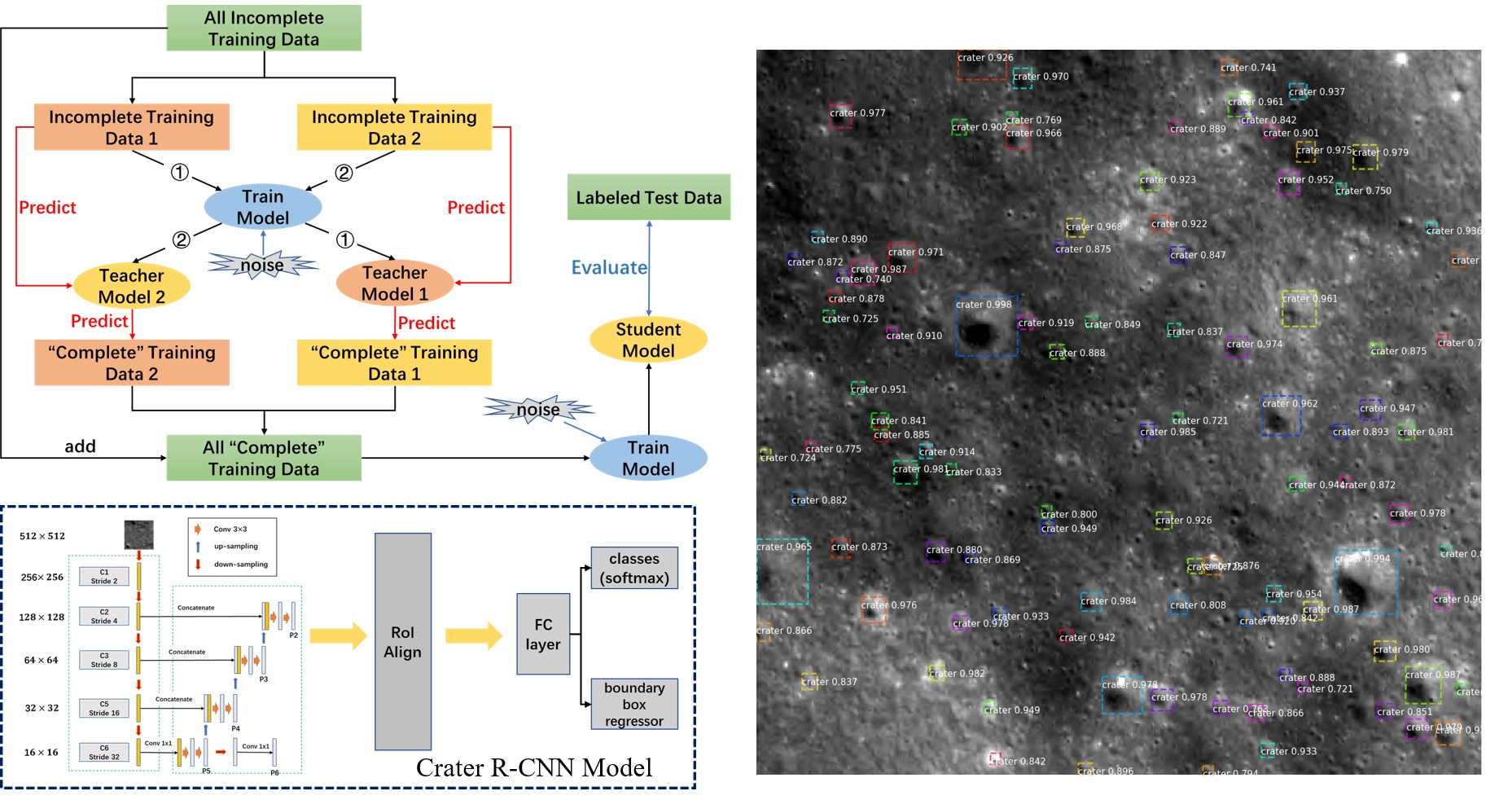
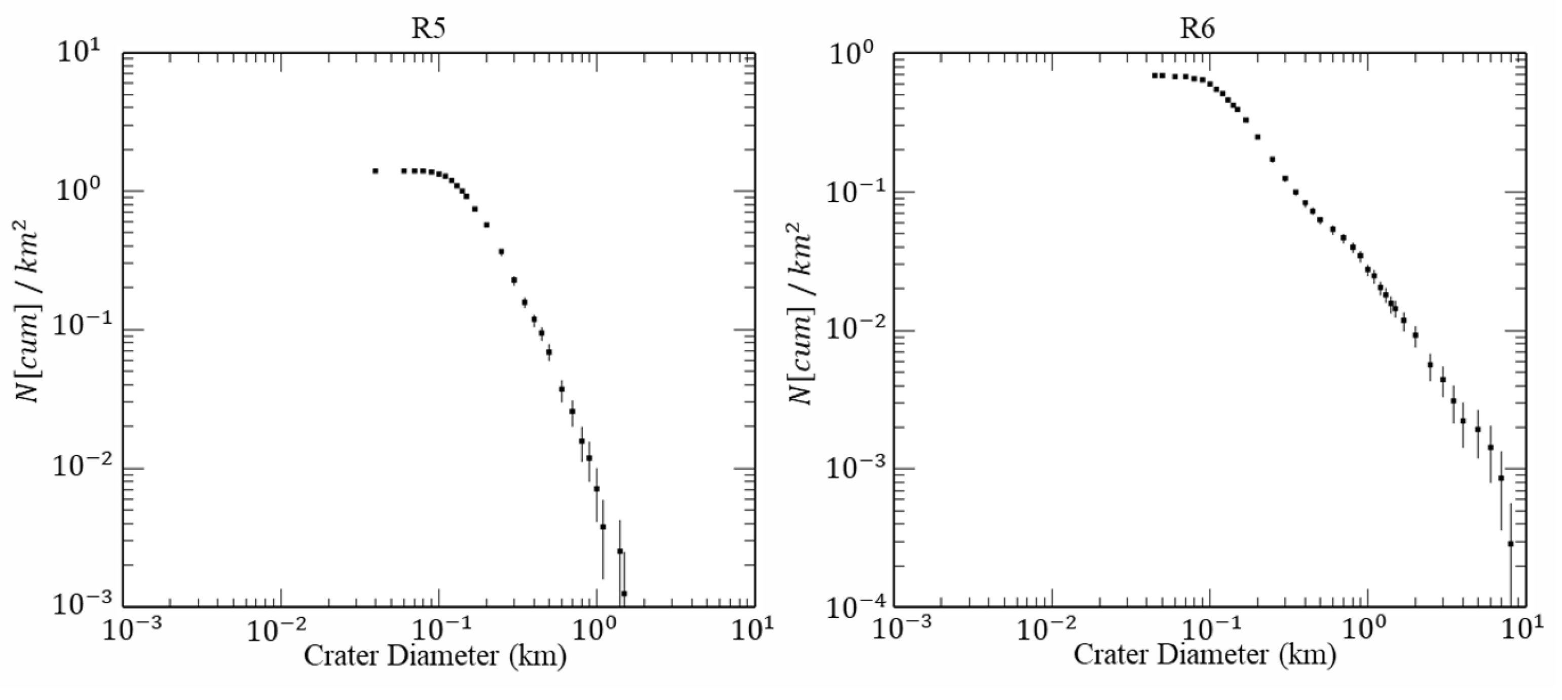
As for the test data set, all of the craters were labeled in R5 and R6. R5 was in Maria, near Mons Rumker, where Chang’E-5 landed in 2020; meanwhile, R6 was in Highland, covering the Highland Ponds. A total of 1105 and 2388 craters were labeled in the R5 and R6 areas, respectively, and their size–quantity distribution is shown in Figure 5. It can be seen, from the figure, that the radius of most craters in the two areas was smaller than 200 m, and the number of craters with a radius larger than 500 m in the R5 area was smaller than that in the R6 area.
2.3. CE-2 DOM Comparison in Highland and Maria
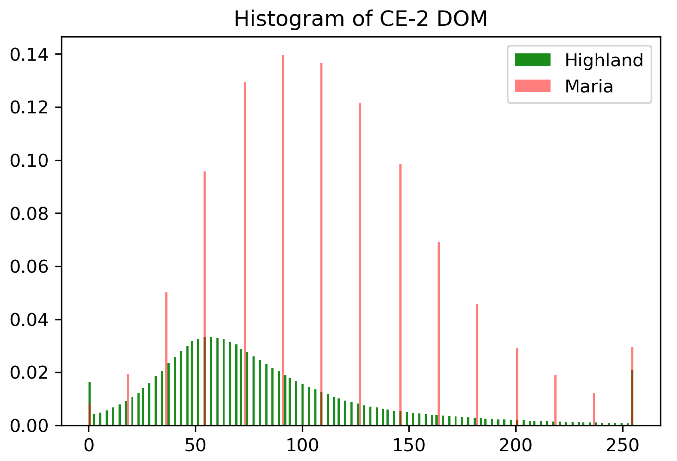
The training data and test data selection in most previous studies has not paid attention to the difference in DOM data for different terrain. Additionally, to further quantitatively compare the differences between lunar Maria and Highland data in the DOM data obtained by CE-2, we prove the necessity of constructing crater samples under different terrain types. We also analyze the generalization ability of the constructed model. Furthermore, to analyze the crater detection performance of the models (see Section 4), the difference between the R5 and R6 CE-2 DOM was compared. As can be seen from Figure 6, the histogram of the pixel values in Maria was more scattered than that for Highland, which means that the data quality was low in Maria. For this reason, it was not easy to label the craters with radius less than 100 m, which led to a large number of missing labels for craters within 100 m radius in the training data.
Additionally, to quantitatively analyze the difference between the Highland and Maria DOM, the gray mean (), gray variance (), information entropy (f), and energy function of gradient (EOG) [38] were calculated, as follows:
where are the height and width of the image, respectively, and is the pixel value;
where i is the value of the pixel and j is the mean value of the neighborhood; and
where are the height and width of the image, respectively, and is the pixel value.
The gray mean, gray variance, information entropy, and EOG reflect the overall radiation status of the image, hierarchical information, information content, and clarity of the image, respectively. In Table 3, the correlation values of image quality are given. The overall radiation status of the image, the hierarchical information of the image gray, and the image clarity of the image of Maria were all higher than those in Highland, except for the information content. In particular, the EOG value in Maria was 624.81, which was nearly five times more than that in Highland (126.14). Therefore, overall, the DOM in Highland was different from that in Maria.
3. Methods
The identification and location extraction of craters essentially comprise a target detection task. Target detection based on deep learning can mainly be divided into one- and two-stage detection frameworks. One-stage detection frameworks, such as YOLO [39,40,41] and SSD [42], rely on the deep feature layer in the network, which has a large receptive field, low precision, and poor performance when detecting small objects. However, two-stage detection frameworks, such as R-CNN, use algorithms to generate a series of candidate boxes as samples, then classify these samples through the use of a fully connected layer, such that high accuracy can be obtained in detecting both small and large objects [43]. The edge of a lunar crater is irregular, and there is often overlap between craters of different sizes. Moreover, most craters are very small in high-resolution imagery, such that a one-stage detection framework cannot meet the crater detection task with high accuracy. Therefore, R-CNN, which has better performance at present, was selected to detect craters in the considered high-resolution DOM. In this Section, to solve the problem of low identification precision and location information extraction in the small crater detection task, the Crater R-CNN model (Section 3.2) is proposed and compared with the popular Mask R-CNN [44] model (Section 3.1). Furthermore, the Two-Teachers Self-training with Noise (TTSN) method (Section 3.3) is proposed for model training, in order to solve the problem of poor model detection performance caused by incomplete crater sample labels in the DOM.
3.1. Mask R-CNN and No-Mask R-CNN Used for Crater Detection
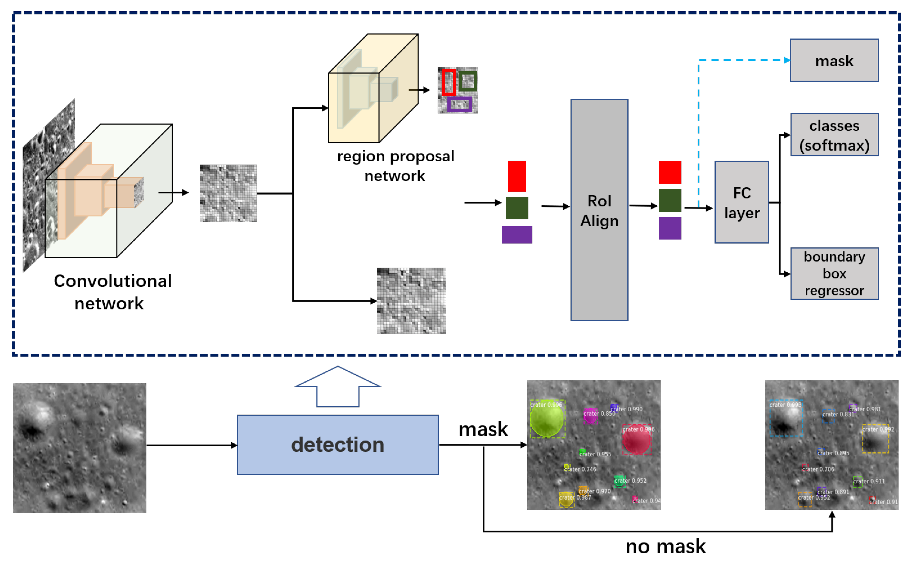
Mask R-CNN, proposed by He Kaiming et al. [44], is a general framework for object detection and instance segmentation. Mask R-CNN is a neural network which generates a series of candidate regions with potential targets, and then classifies, regresses, and segments each region, according to the characteristics of the candidate regions. Mask R-CNN was used to detect craters using DOM data, and the instance segmentation of craters was realized. The overall framework of using Mask R-CNN (as well as no-Mask R-CNN, see below) to detect craters, is shown in Figure 7. First, DOM data are input to the deep network, in order to extract the semantic information of craters. As a result, feature graphs with different sizes are created, including the spatial and semantic information of craters with different sizes. Then, a Region Proposal Network (RPN) implements the classification and regression operations for craters in different feature maps. The probability of a crater being included in the input anchor is obtained by classification, and the location information of the anchor is preliminarily extracted by regression. Furthermore, after classifying and regressing the target boxes, the candidate boxes are screened twice. The former are sorted according to the probability of each target box containing a crater, and the latter solves the IoU for the selected craters and the real craters used for training. Region of Interest Alignment (RoIAlign) is used to realize the accurate extraction of crater target boxes, and finally completes the screening of those target boxes containing craters. According to the size of the selected candidate box, the corresponding feature layer is selected for binary classification of the crater and regression of the box position information, and the real pixel position of the crater is obtained. At the same time, instance segmentation of the crater target is carried out. In the whole process, the cross-entropy loss function is used for classification, and the smooth L loss function is used for regression.
Furthermore, the segmentation module was removed to obtain no-Mask R-CNN, which has a similar overall structure to Faster R-CNN [45]. Ali DIB et al. [32] have applied Mask R-CNN to detect the craters in a DEM, demonstrating it as a good semi-supervised learning-based model. While the training target is a circle in the ideal state, mask R-CNN can still segment non-circular polygons, which are closer to the shape of real craters. Therefore, we further compared whether adding instance segmentation is conducive to crater detection in the case of the inaccurately labeled rims in the DOM. In Figure 7, the instance segmentation operation in Mask R-CNN is removed. Thus, it is called no-Mask R-CNN. Compared with the original model, no-Mask R-CNN has no instance segmentation function, while the rest of the model is the same, such that it can achieve faster training and detection.
3.2. Crater R-CNN
Crater R-CNN is improved from Faster R-CNN, which was first proposed by Ren, S. [45]; however, it does not include an instance segmentation step. Faster R-CNN is mainly divided into two stages: the first stage, called a Region Proposal Network (RPN), proposes candidate object bounding boxes. The second stage of Faster R-CNN—which is, in essence, Fast R-CNN [46]—extracts features, using the RoIPool operation, for each candidate box and performs classification and bounding box regression. However, in the process of feature extraction, it lacks low-level features and loses local detail information; that is, it lacks the information required for extraction of craters, leading to poor detection performance for small craters. In addition, although the calculation of the RoIPool operation in Faster R-CNN is fast, there may be a large deviation in mapping to the real position of the original image, which is caused by rounding of the position of the target box on the small feature map.
Based on this, Crater R-CNN was proposed, which is efficient in terms of feature extraction, as well as being more accurate in terms of identification and location. To extract deeper crater features in the DOM, the ResNet 101 layer (instead of VGG) was used to extract features. In addition, to solve the inaccurate target box location problem, the ROI pooling layer was replaced by the ROIAlign, such as in Mask R-CNN, and the bilinear interpolation method was used to obtain the pixel coordinates of the floating-point numbers in the image, thus eliminating the error of the model related to obtaining the target location.
As shown in Figure 8, to obtain more comprehensive spatial semantic information of craters, the related operation in the up-sampling process was further improved. In the feature extraction process, Mask R-CNN adopts a feature pyramid network module. First, the feature map of the previous layer is convolved to eliminate the aliasing effect and extract the target spatial information, then it is added to the feature map obtained by up-sampling. The above operations still cannot effectively extract the features of craters, due to the overlapping, degradation, and size variation of craters. Therefore, compared with Mask R-CNN, the skip connection operation is used to merge channels (instead of add operations), in order to fuse the feature information. Additionally, in the process of up-sampling, compared with the add operation in the channel, the skip connection method increases the resolution of image detail features; furthermore, skip connections are helpful in eliminating singularities and in deep network training [47,48], thus promoting the detection of craters and the extraction of location information.
3.3. Two-Teachers Self-Training with Noise (TTSN)
A self-training method can realize semi-supervised deep learning and solve the problem of low accuracy caused by a lack of labeled data. An obvious problem related to lunar crater data is not the lack of a labeled data set, but the incompleteness of labeled data sets, which can have a great influence on crater detection. Traditional self-training, based on the single-teacher model, can solve the problem relating to a lack of labeled data. First, a single learner or integrated learning model is trained to label all or most of the unlabeled samples, and then “pseudo-labeled” data are combined with the original labeled data, in order to train the model or other models. Semi-supervised methods based on “pseudo-labeled” data usually need the model to be trained repeatedly, leading to poor generalization performance and over-fitting [49]. In addition, this method may create a large amount of crater training data: as it requires extra unlabeled samples for training, the number of training samples will be increased.
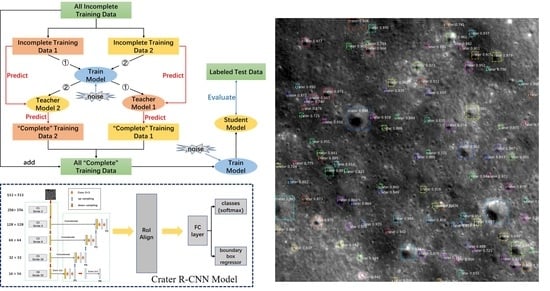
To solve the above problem of incomplete crater labels, the Two-Teachers Self-training with Noise (TTSN) method is proposed. Algorithm 1 gives the detailed steps of TTSN, and Figure 9 shows an overview of TTSN. To reduce the amount of training data, first of all, the incomplete training set is split into two parts. To obtain a teacher model with higher robustness, Gaussian noise is added into the two incomplete training images. The models are consequently trained, in order to obtain teacher model 1 and teacher model 2. Then, we exchange the original training data between the two models. We do not add noise, and input the data into the teacher model as unlabeled data, thus obtaining two sets of prediction results. The craters predicted by the teacher models with confidence greater than 0.75 are used as pseudo-labeled data, and the crater locations are exported to a text file, which is further compared with the original labeled crater data. The additionally identified craters are fused as label information. Furthermore, the training samples are generated according to the “complete” position information of the crater, and noise is added into the student model. Differing from traditional self-training methods, the original training data are not integrated here. Due to the semi-supervised ability of the model, the original crater to be predicted can be extracted with high precision. By improving the confidence of the predicted target, we can obtain the target with high confidence as the “pseudo-labeled” data, which increases the model’s crater detection accuracy. During the training process, it is necessary to re-train the student model using the “pseudo-labeled” data obtained from the two teacher models. Finally, we use the test data to evaluate the student model.
| Algorithm 1: Two-Teachers Self-training with Noise. |
| Data: Incomplete labeled images divided into and . Step 1: Train the teacher models and , which minimize the cross-entropy loss and smooth L loss on incomplete labeled images: , . Step 2: Use two normal (i.e., non-noisy) teacher models to generate pseudo-labels. The new pseudo-labels with confidence level higher than are selected and fused with manual labels. Here, indicates a confidence of 0.75. Step 3: Train a better student model, , which minimizes the cross-entropy loss and smooth L loss on labeled and pseudo-labeled images. |
3.4. Model Training
All of the obtained data sets were fed into the above models, which were constructed using TensorFlow. A total of 5000 images were generated from R1—4, of which 4000 images were randomly selected for model training, and the remaining 1000 images were used for model validation, in order to obtain model parameters. In model training, to improve the generalization ability of the model, horizontal and vertical flip strategies were randomly applied to the training data. To obtain the hyper-parameters of Crater R-CNN with TTSN, Crater R-CNN was trained first. As for the training and hyper-parameters of Mask R-CNN and no-Mask R-CNN, we used the same procedure as in [32]. In the process of training, the IoU was mainly used to filter the bounding boxes. First, the bounding boxes with IoU between bounding boxes and highest confidence target greater than 0.7 were deleted through the non-maximum suppression method [44]. Then, the IoU values between the bounding boxes preserved in the previous step and ground truth were calculated, which were used to divide the samples into positive and negative samples for training (IoU ≥ 0.6, positive samples; IoU < 0.4, negative samples; and 0.4 ≤ IoU < 0.6 was not considered). A multi-task loss on each sampled RoI was defined as L = L + L. The classification loss, L, and bounding-box loss, L, were identical to those defined in [46]. To speed up the minimization of the loss value, the Adam optimizer was used to update the network weights, while the backbone of the four models was ResNet101, which was pre-trained using ImageNet data [26]. Defining an “epoch” as a single pass through the entire training set and “batch size” as the number of examples seen per back-propagation gradient update, each model was trained for 10 epochs with a batch size of 2, which meant that the final loss value was less than 0.1 and the loss change between the last two epochs was less than 0.001. The model was trained with different hyper-parameters, and those which led to the minimum loss value—according to the results on the verification data set—were chosen as the best hyper-parameters. Finally, we determined a set of hyper-parameters for Crater R-CNN (see the Appendix A). The names of all hyper-parameters were the same as those given here (https://github.com/matterport/Mask_RCNN (accessed on 15 July 2021).
After determining the hyper-parameters, the TTSN method was used to train Crater R-CNN, thus creating the new model: Crater R-CNN with TTSN. Thus, the hyper-parameters of the following models were the same as those in Crater R-CNN. A total of 2500 images were randomly selected from the 5000 images and Gaussian noise with a mean of 0 and 1 variance was added, in order to train Crater R-CNN and obtain teacher model 1. In the same way, teacher model 2 was trained using the other half of the data. To obtain crater “pseudo-labels”, the data of each teacher model was used as input to the other for crater detection without noise, and craters with identification probability greater than 0.75 were extracted from each image. By fusing the “pseudo-label” and the ground truth in each image, 5000 new training images were obtained. The final number of crater labels in these images was about 1.1 times the original number of craters. Finally, Gaussian noise with a mean of 0 and variance of 1 was added to the 5000 images, which were then used for model training, in order to obtain the student model.
4. Results
To test the performance of Mask R-CNN, no-Mask R-CNN, Crater R-CNN, and Crater R-CNN with TTSN, all of the test image data were divided into 512 × 512 pixel blocks and input into the detection models. Additionally, the following parameters were defined, in order to evaluate the detection accuracy:
where P is the precision, R is the recall and score is a comprehensive evaluation index. , , and are the number of true positives, false positives, and false negatives, respectively. As the crater with 256 pixels can always be displayed completely in one image block, we only kept craters with diameter ≤256 pixels (1792 m) in the detection result.
4.1. Crater Detection Post-Processing
After model training is completed, the accuracy of a model needs to be tested. On one hand, it was necessary to detect the craters in the whole test area and obtain the projection coordinates of the craters. On the other hand, it is necessary to remove duplicate craters and judge whether the craters are detected correctly.
In the process of cutting R5 and R6 into image blocks (see Section 2.2), we left a half-intersection between adjacent images, such that the model could detect the craters in the research area. These data were fed into the deep learning models as a test set, in order to assess the detection accuracy of the models. To improve the accuracy of crater detection, the bounding boxes with confidence greater than 0.75 were preserved, the bounding boxes with IoU between bounding boxes and highest confidence bounding box greater than 0.3 were deleted using non-maximum suppression method and, finally, only the bounding boxes with the highest confidence were obtained. At the same time, duplicate detected craters in a single image block were removed. As a result of the detection step, the detected craters were presented as a rectangle with an image pixel coordinate. The diameter (D) of the detected crater was defined as the average of the length and width of the rectangle, and the location was the center point of the rectangle. To obtain the coordinates, the image pixel coordinates should be transformed into a projection coordinate, using Equations (8)–(10), following which a projection function can be used to obtain the geographic coordinates. All of the transformation parameters were stored in an image file, which was obtained using the osgeo package in Python.
where , represents the projection coordinate of the upper-left corner of the image; and represent the horizontal and vertical resolutions, respectively; , is the image pixel coordinate; and , is the projection coordinate.
The duplicate craters in the results were mainly generated by regions duplicated during image clipping. Additionally, on the boundary of the image, duplicate craters were produced with little difference in location and size. Therefore, in the post-processing step, an overlapping index () and a simulation index () were used to identify duplicate craters. As a result, the largest crater was the retained, and the others were deleted. Finally, we evaluated the accuracy, for which the final results were compared with the ground truth in the test set. When Equations (11) and (12) were satisfied, it was judged as a true positive result.
where and are the radii of the craters, and the distance is measured between the center points of the craters. After testing, when is 1 and is 0.25, all of the duplicate craters can be deleted.
4.2. Accuracy Evaluation
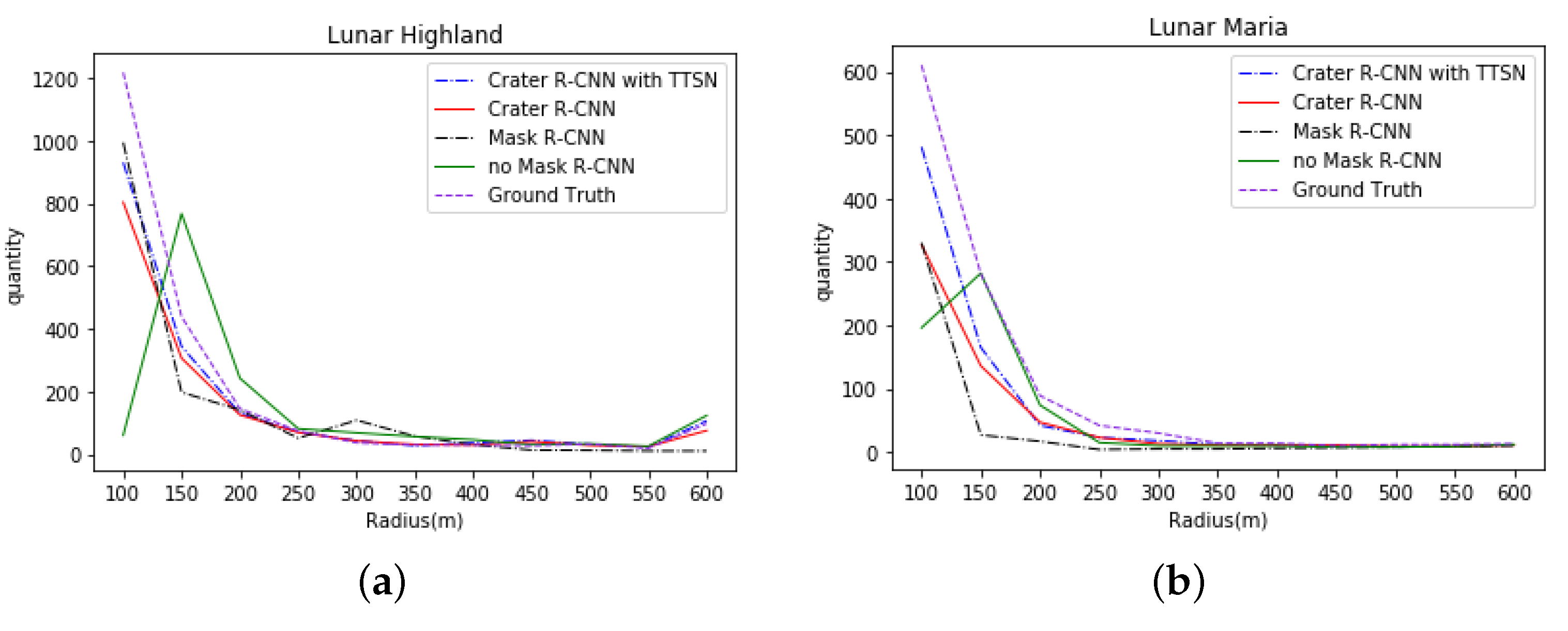
In the model test, Mask R-CNN, no-Mask R-CNN, Crater R-CNN, and Crater R-CNN with TTSN detected 1941, 2055, 2070, and 2464 craters, respectively, in the Highland and Maria regions. Figure 10 shows the distribution of the number of craters identified by the above methods and manual labeling at different scales, and it can be seen that the number of craters decreased with the increase of radius. However, the number of small detected craters (radius < 150 m) was less than that of those which were labeled. Meanwhile, no-Mask R-CNN detected fewer small craters (radius < 100 m) and more medium craters (100 m < radius < 150 m) in Highland. In Maria, no-Mask R-CNN found fewer small craters (radius < 100 m) only. It can be seen, from Figure 11, that the detection result of no-Mask R-CNN for small craters was larger than the true number of craters. Thus, the use of no-Mask R-CNN led to crater rim detection errors.
Table 4 presents the accuracy evaluation for the different crater detection models. The overall accuracy evaluation was based on the detected results in Highland and Maria regions. The table shows that Crater R-CNN with TTSN had the best overall precision (P = 90.5%), highest overall recall (R = 63.5%), and best comprehensive evaluation index (F = 74.7%). The overall accuracy of Crater R-CNN (R = 49.5%, P = 83.9%, F = 62.2%), no-Mask R-CNN(R = 43.5%, P = 74.3%, F = 54.9%), and Mask R-CNN (R = 36.9%, P = 66.6%, F = 47.5%) became consecutively smaller. The accuracies in Highland and Maria regions were consistent with the overall accuracy, indicating that the above models could effectively overcome the topographic differences. Compared with the other three models, the recall rate of the Crater R-CNN with TTSN was significantly higher, which means that Crater R-CNN with TTSN produced a large number of correct “pseudo-labels” and had a strong generalization performance. In the table, we further provide the average IoU between the detected craters and the ground truth, as well as the ratio of the radii of detected craters (Pre_R) to those of the ground truth (R). It can be seen, from the results, that the IoUs of Crater R-CNN and Crater R-CNN with TTSN were better, while the IoU of Mask R-CNN was the lowest. Thus, Mask R-CNN and no-Mask R-CNN performed poorly when locating craters. From the perspective of the radius ratio, the radii of craters predicted by Mask R-CNN were lower, while the radii of craters predicted by no-Mask R-CNN were larger than those predicted by other methods. Therefore, no-Mask R-CNN, as shown in Figure 11 and Figure 12, was quite different from the other methods.
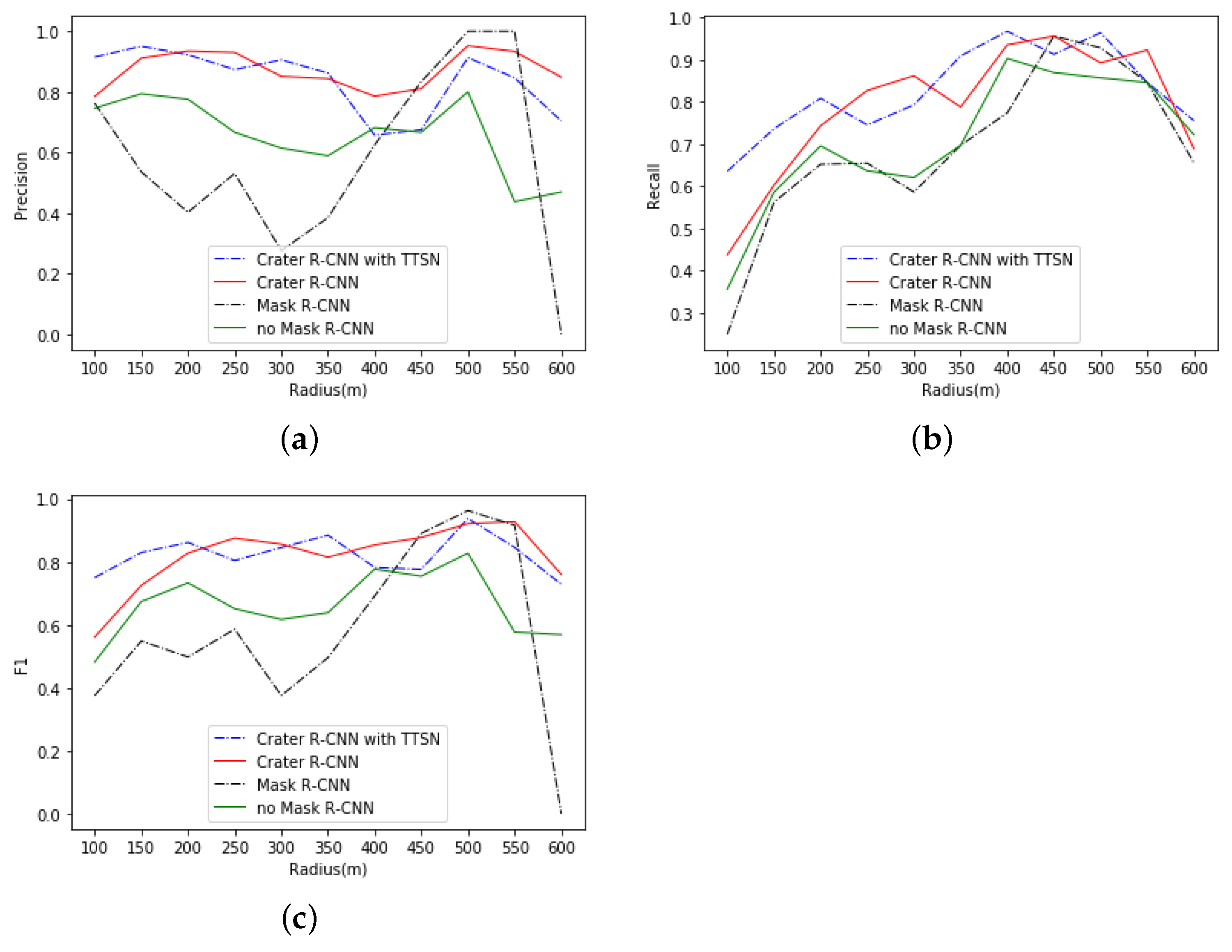
To understand the effect of scale on the models, statistical analysis of the accuracy was carried out under different radii. Overall, Figure 12 shows that R, P, and F were not stable. When the radius was less than 100 m or more than 600 m, R was low, while it was high between 100 and 600 m. The P and F values were consistent with each other. The value of P for Mask R-CNN was low within 400 m of radius and increased rapidly between 400–550 m, indicating that Mask R-CNN was more unstable. The P and F values of Crater R-CNN and Crater R-CNN with TTSN were higher than 0.8 when the radius was within 350 m. Almost all the P and F values of Crater R-CNN and Crater R-CNN with TTSN were larger than those of Mask R-CNN and no-Mask R-CNN. As can be seen from Figure 12, in all dimensions and indicators, Crater R-CNN with TTSN had better performance. According to the number and distribution of craters, we divided them into three categories, according to radius: radius < 100 m, 100 m ≤ radius < 200 m, and radius ≥ 200 m. In Table 5, the accuracy of crater detection under these three sizes is provided. As the resolution of CE-2 DOM is 7 m/pixel, the craters with radius less than 100 m occupied less pixels, and there were a lot of missing crater labels, such that the detection accuracy of craters with R < 100 m was relatively low, but the detection accuracy of craters with radius more than 100 m was relatively high and consistent. With the improvement of DOM data resolution, Crater R-CNN with TTSN can meet the requirements of crater detection within 1 km.
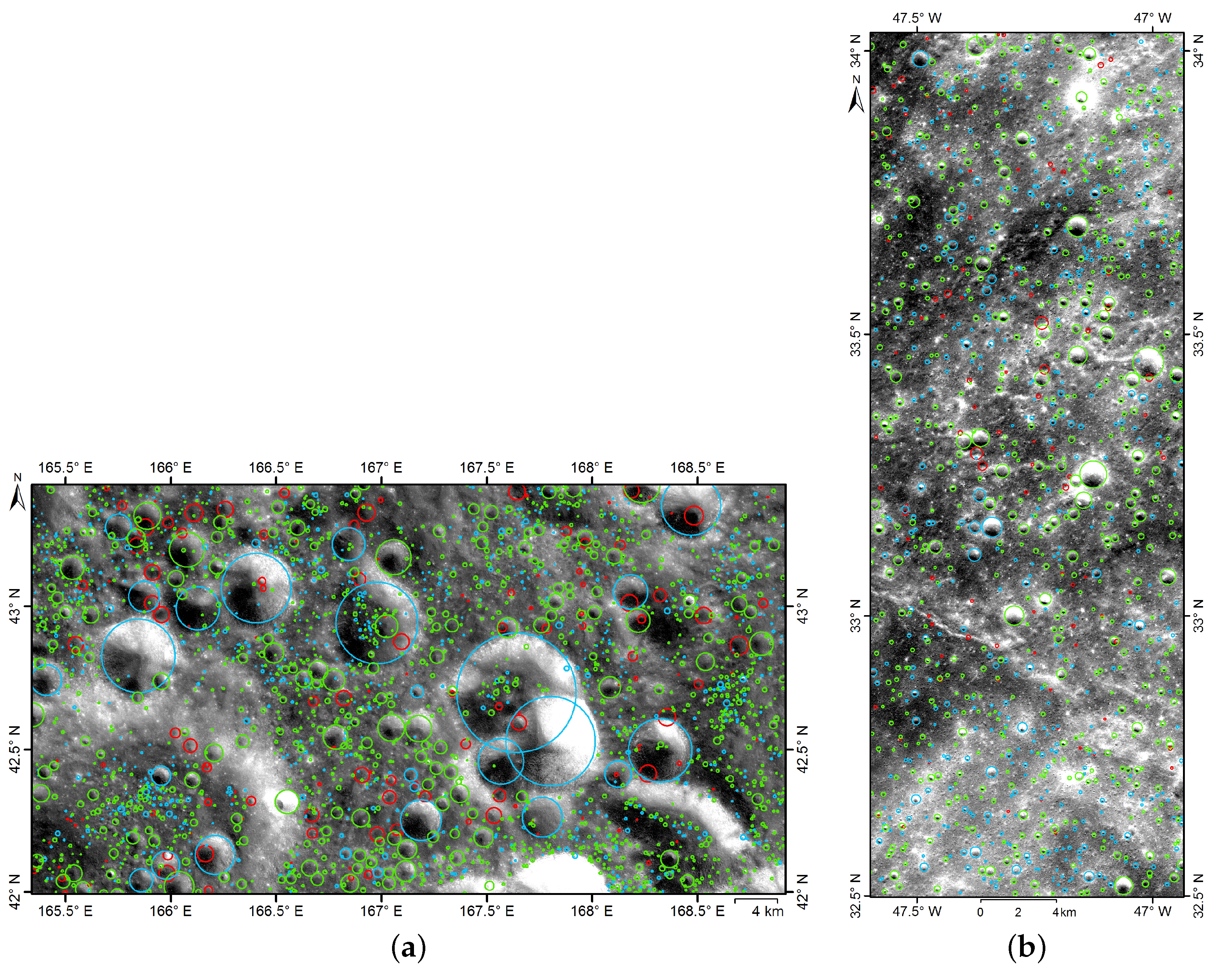
Figure 13 shows the spatial distribution of the craters detected by Crater R-CNN with TTSN in the Highland and Maria regions. There were more small true negatives (blue) than large ones. However, the former were mainly located in areas with high crater density. The distribution of the false positives (red) was relatively random, and its scale was mainly medium-sized. Therefore, as shown in Figure 11, the value of P for Crater R-CNN with TTSN was relatively low at medium scales. The true positives (green) covering the small and middle scale were mainly found at the bottom of complex craters, indicating that Crater R-CNN with TTSN has strong robustness.
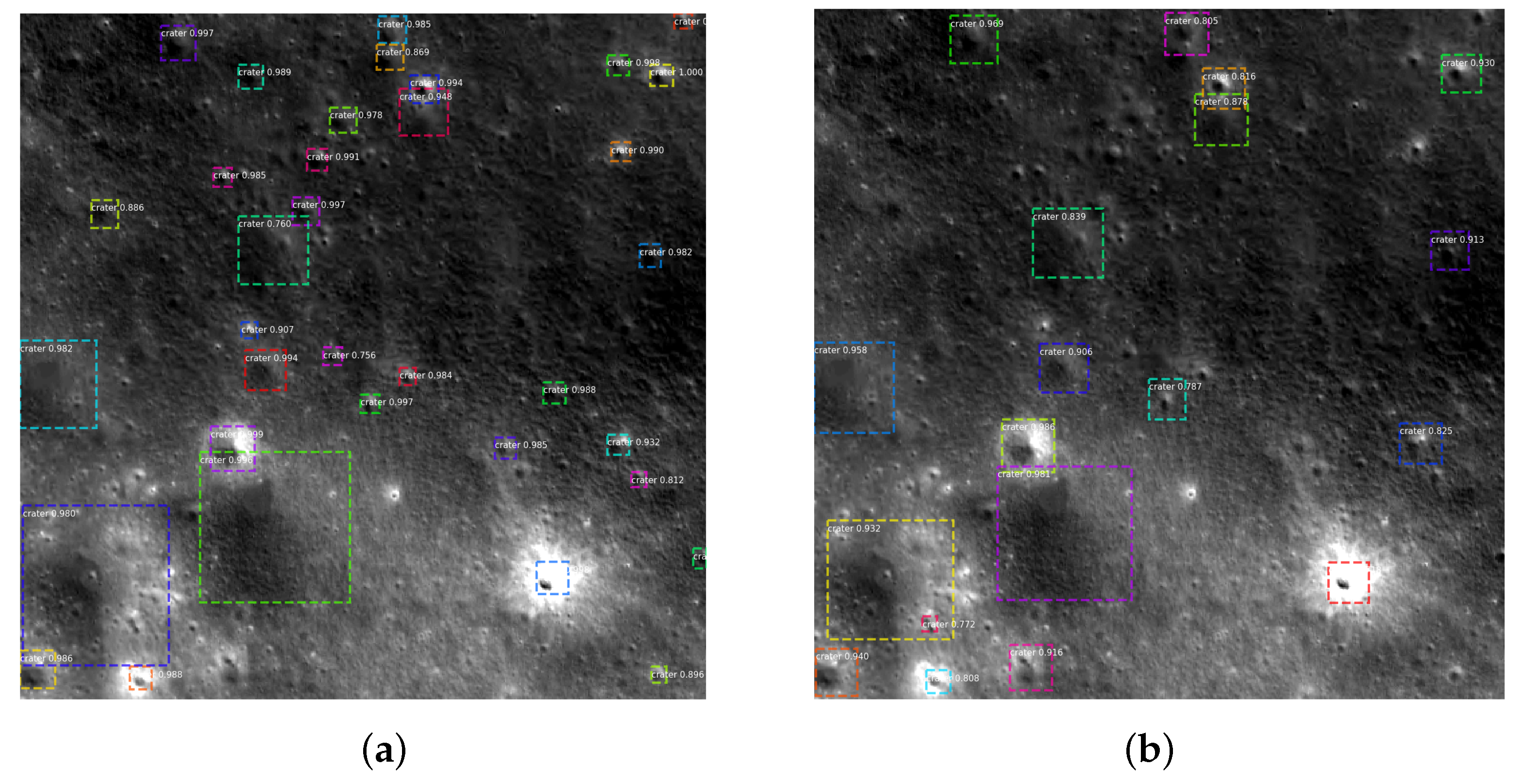
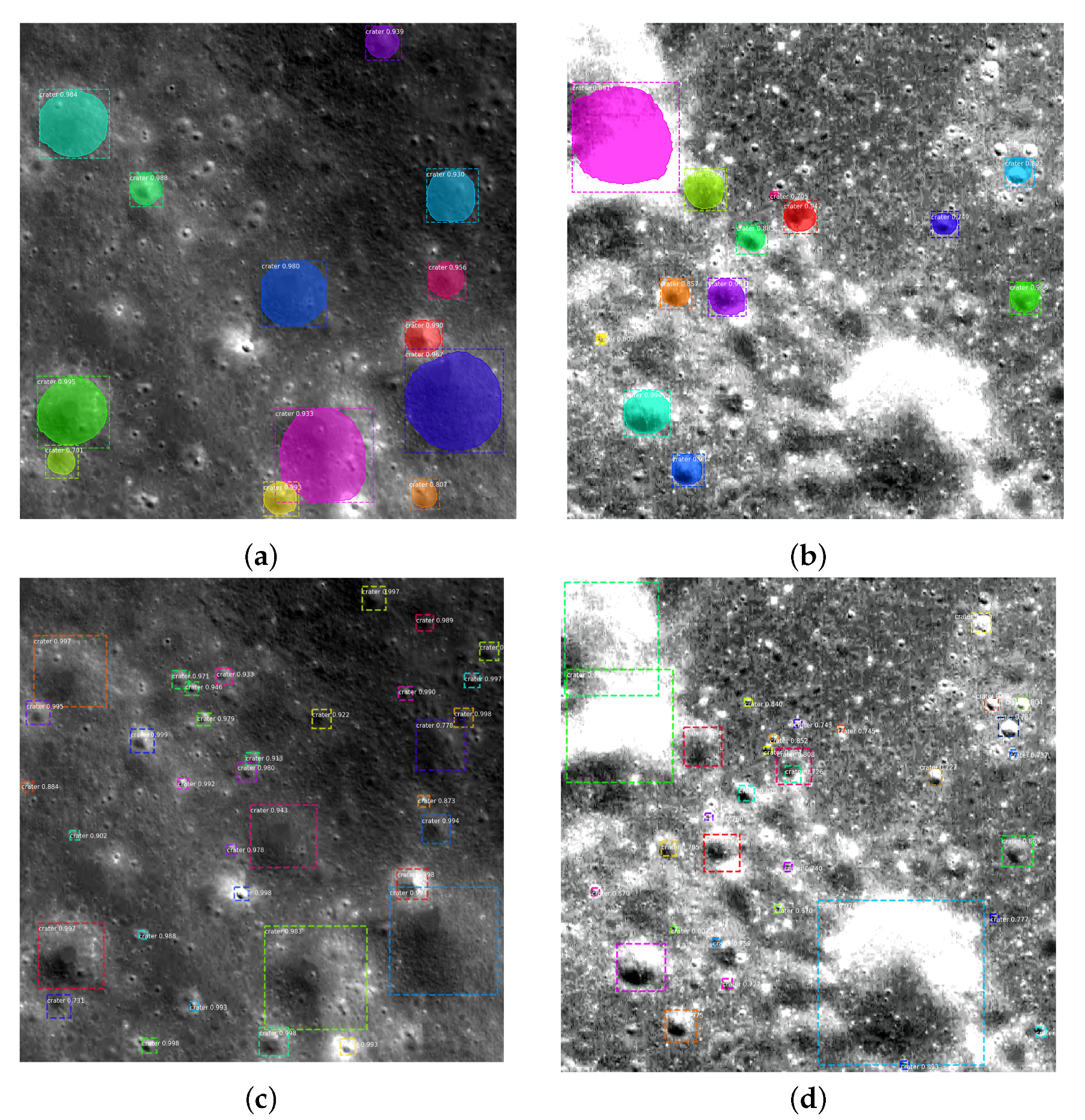
To further analyze the effect of instance segmentation on crater detection using DOM, the detection results of Crater R-CNN with TTSN and Mask R-CNN were randomly selected in Highland and Maria. Figure 14 shows that more small craters were detected by Crater R-CNN with TTSN than Mask R-CNN. Due to label errors at crater rims and the unclear rims of craters in the DOM, the rims of craters segmented by Mask R-CNN were inaccurate. Figure 14a,c show that Crater R-CNN with TTSN detected a large number of small craters in Highland, but Mask R-CNN missed many small ones. In Maria, the image data quality was poor, as mentioned in Section 2.3. As a result, Mask R-CNN missed a large number of small craters, incorrectly detected overlapping craters in the upper left corner, and did not detect large craters located at the bottom of the image. However, Crater R-CNN with TTSN could effectively distinguish overlapping craters, small craters, and large craters, as shown in Figure 14d. Therefore, Crater R-CNN with TTSN had better generalization ability and was more suitable for crater detection using DOM.
5. Summary and Conclusions
Based on an investigation of CE-2 DOM data and various crater detection methods, a new small crater detection method, called Crater R-CNN with TTSN, was proposed in this paper. Several crater samples in the Highland, Maria, low-altitude, and medium–high-latitude areas were labeled, in order to train and evaluate Mask R-CNN, no-Mask R-CNN, Crater R-CNN, and Crater R-CNN with TTSN models. The results indicated that Crater R-CNN with TTSN had the highest overall accuracy (P = 90.5%, R = 63.5%, F1 = 74.7%), and had better localization ability (IoU = 88.6%) and size estimation (Pre_R/R = 96.4%). The accuracy of the proposed model in the Highland and Maria regions was consistent with the overall accuracy, and the recall of Crater R-CNN with TTSN was higher than that of the other three models, as the proposed method generated a large number of “pseudo-labels” to overcome the problem of missing labels, has strong generalization performance, and is a high-precision semi-supervised learning method. In addition, the use of a segmentation network is not conducive to the detection of craters in DOM imagery, such that it was difficult for no-Mask R-CNN to obtain the true size of small craters. Therefore, Crater R-CNN with TTSN could accurately detect craters with a radius of more than 100 m, as well as accurately locating the craters and estimating their size.
With the acquisition of high-resolution imagery by CE-2, LRO, and Selene, as well as that obtained by future missions, Crater R-CNN with TTSN provides a new way to detect small craters within 1 km diameter using DOM—instead of DEM (with low resolution)—making it possible to effectively detect small lunar craters and to build lunar crater databases at different scales. New lunar craters can be used to analyze the distribution of lunar craters and modify the accurate geological age of the Moon, which may provide support in answering some questions about its origin and evolution. Additionally, small craters can be used for landing site selection and navigation on the Moon in the future. However, the samples used in this paper did not cover the polar regions—especially the permanent shadow areas—and the sample data sources were limited to CE-2 DOM. Therefore, future research should focus on improving the generalization capability of the model and expanding the diversity of the sample data.
Author Contributions
Conceptualization, L.M. and S.Z.; methodology, S.Z. and L.M.; formal analysis, S.Z., L.M. and L.X.; resources, S.Z., L.X. and W.Z.; wirting—original draft preparation, S.Z. and L.M.; writing—review and editing, L.M. and S.Z.; supervision, L.M.; project administration, L.M. and W.Z.; funding acquisition, L.M. and W.Z.; mapping, L.M., S.Z. and L.X. All authors have read and agreed to the published version of the manuscript.
Funding
This research was funded by The National High Technology Research and Development Program of China (No. 2010AA122202).
Data Availability Statement
CE-2 DOM data are available at https://moon.bao.ac.cn/searchOrder_pdsData.search (accessed on 15 July 2021).
Acknowledgments
We thank the Ground Research & Applications System (GRAS) of the Chinese Lunar Exploration Project (CLEP) for providing data. Careful comments given by the anonymous reviewers helped to improve the manuscript.
Conflicts of Interest
The authors declare no conflict of interest.
Sample Availability
Samples of training data, testing data, and code are available from the authors.
Abbreviations
The following abbreviations are used in this manuscript:
| DEM | Digital Elevation Model |
| DOM | Digital Orthophoto Map |
| CE-2 | Chang’E-2 |
| LRO | Lunar Reconnaissance Orbiter |
| CDA | Crater Detection Algorithm |
Appendix A
We adopted the following model hyper-parameters in our work:
BACKBONE : resnet101
BACKBONE_STRIDES : [4, 8, 16, 32, 64]
BATCH_SIZE : 2
BBOX_STD_DEV : [0.1 0.1 0.2 0.2]
COMPUTE_BACKBONE_SHAPE : None
DETECTION_MAX_INSTANCES : 400
DETECTION_MIN_CONFIDENCE : 0.75
DETECTION_NMS_THRESHOLD : 0.3
FPN_CLASSIF_FC_LAYERS_SIZE : 1024
GPU_COUNT : 1
GRADIENT_CLIP_NORM : 5.0
IMAGES_PER_GPU : 2
IMAGE_CHANNEL_COUNT : 1
IMAGE_MAX_DIM : 512
IMAGE_META_SIZE : 14
IMAGE_MIN_DIM : 512
IMAGE_MIN_SCALE : 0
IMAGE_RESIZE_MODE : square
IMAGE_SHAPE : [512, 512, 1]
LEARNING_MOMENTUM : 0.9
LEARNING_RATE : 0.001
LOSS_WEIGHTS : The proportion is the same
MAX_GT_INSTANCES : 400
NUM_CLASSES : 2
POOL_SIZE : 7
POST_NMS_ROIS_INFERENCE : 1000
POST_NMS_ROIS_TRAINING : 2000
PRE_NMS_LIMIT : 6000
ROI_POSITIVE_RATIO : 0.33
RPN_ANCHOR_RATIOS : [0.5, 1, 2]
RPN_ANCHOR_SCALES : (16, 32, 64, 128, 256)
RPN_ANCHOR_STRIDE : 1
RPN_BBOX_STD_DEV : [0.1 0.1 0.2 0.2]
RPN_NMS_THRESHOLD : 0.7
RPN_TRAIN_ANCHORS_PER_IMAGE : 600
TOP_DOWN_PYRAMID_SIZE : 256
TRAIN_BN : False
TRAIN_ROIS_PER_IMAGE : 600
WEIGHT_DECAY : 0.0001
References
- Luo, L.; Mu, L.; Wang, X.; Li, C.; Ji, W.; Zhao, J.; Cai, H. Global detection of large lunar craters based on the CE-1 digital elevation model. Front. Earth Sci. 2013, 7, 456–464. [Google Scholar] [CrossRef]
- Wilhelms, D.E.; Mccauley, J.F.; Trask, N.J. The Geologic History of the Moon. USA Geol. Surv. Prof. Pap. 1987, 1384, 283–292. [Google Scholar]
- Neukum, G.; Konig, B.; Arkani-Hamed, J. A study of lunar crater size-distributions. Moon 1975, 12, 201–229. [Google Scholar] [CrossRef]
- Craddock, R.A.; Maxwell, T.A.; Howard, A.D. Crater morphometry and modification in the Sinus Sabaeus and Margaritifer Sinus regions of Mars. J. Geophys. Res. Planets 1997, 102, 13321–13340. [Google Scholar] [CrossRef] [Green Version]
- Barlow, N.G.; Bradley, T.L. Martian craters: Correlations of ejecta and interior morphologies with diameter, latitude, and terrain. Icarus 1990, 87, 156–179. [Google Scholar] [CrossRef]
- Downes, L.M. Lunar Orbiter State Estimation Using Neural Network-Based Crater Detection; Massachusetts Institute of Technology: Cambridge, MA, USA, 2020. [Google Scholar]
- Blagg, M.A.; Müller, K.; Wesley, W.H.; Saunder, S.A.; Franz, J. Named Lunar Formations; P. Lund, Humphries: London, UK, 1935. [Google Scholar]
- Arthur, D.W.G.; Agnieray, A.P.; Horvath, R.A.; Wood, C.A.; Chapman, C.R. The System of Lunar Craters, Quadrant I. Commun. Lunar Planet. Lab. 1964, 2, 71–78. [Google Scholar]
- Arthur, D.W.G.; Agnieray, A.P.; Horvath, R.A.; Wood, C.A.; Chapman, C.R. The System of Lunar Craters, Quadrant II. Commun. Lunar Planet. Lab. 1965, 3, 1–2. [Google Scholar]
- Arthur, D.W.G.; Agnieray, A.P.; Pellicori, R.A.; Wood, C.A.; Weller, T. The System of Lunar Craters, Quadrant III. Commun. Lunar Planet. Lab. 1965, 3, 61–62. [Google Scholar]
- Arthur, D.W.G.; Pellicori, R.H.; Wood, C.A. The System of Lunar Craters, Quadrant IV. Commun. Lunar Planet. Lab. 1966, 5, 1–2. [Google Scholar]
- Wood, C.A.; Anderson, L. New morphometric data for fresh lunar craters. In Proceedings of the Lunar and Planetary Science Conference 1978, Houston, TX, USA, 13–17 March 1978; pp. 3669–3689. [Google Scholar]
- Rodionova, Z.F.; Skobeleva, T.P.; Karlov, A.A. A Morphological Catalogue of Lunar Craters. Lunar Planet. Sci. 1985, 16, 706–707. [Google Scholar]
- Head, J.W., 3rd; Fassett, C.I.; Kadish, S.J.; Smith, D.E.; Zuber, M.T.; Neumann, G.A.; Mazarico, E. Global distribution of large lunar craters: Implications for resurfacing and impactor populations. Science 2010, 329, 1504–1507. [Google Scholar] [CrossRef]
- Salamuniccar, G.; Loncaric, S.; Grumpe, A.; Wohler, C. Hybrid method for crater detection based on topography reconstruction from optical images and the new LU78287GT catalogue of Lunar craters. Adv. Space Res. 2014, 53, 1783–1797. [Google Scholar] [CrossRef]
- Öhman, T. LPI Crater Database; Lunar & Planetary Institute: Houston, TX, USA, 2015. [Google Scholar]
- Jiao, W.; Weiming, C.; Chenghu, Z. A Chang’E-1 global catalog of lunar craters. Planet. Space Sci. 2015, 112, 42–45. [Google Scholar]
- Povilaitis, R.Z.; Robinson, M.S.; van der Bogert, C.H.; Hiesinger, H.; Meyer, H.M.; Ostrach, L.R. Crater density differences: Exploring regional resurfacing, secondary crater populations, and crater saturation equilibrium on the moon. Planet. Space Sci. 2018, 162, 41–51. [Google Scholar] [CrossRef]
- Robbins, S.J. A New Global Database of Lunar Impact Craters >1–2 km: 1. Crater Locations and Sizes, Comparisons With Published Databases, and Global Analysis. J. Geophys. Res. 2019, 124, 871–892. [Google Scholar] [CrossRef]
- Delatte, D.M.; Crites, S.T.; Guttenberg, N.; Yairi, T. Automated crater detection algorithms from a machine learning perspective in the convolutional neural network era. Adv. Space Res. 2019, 64, 1615–1628. [Google Scholar] [CrossRef]
- Stepinski, T.F.; Mendenhall, M.P.; Bue, B.D. Machine cataloging of craters on Mars. Icarus 2009, 203, 77–87. [Google Scholar] [CrossRef]
- Urbach, E.R.; Stepinski, T.F. Automatic detection of sub-km craters in high resolution planetary images. Planet. Space Sci. 2009, 57, 880–887. [Google Scholar] [CrossRef]
- Yang, J.; Kang, Z. Bayesian network-based extraction of lunar craters from optical images and DEM data. Adv. Space Res. 2019, 63, 3721–3737. [Google Scholar] [CrossRef]
- Machado, M.; Bandeira, L.; Pina, P. Automatic crater detection in large scale on lunar Maria. In Proceedings of the 46th Lunar and Planetary Science Conference (2015), The Woodlands, TX, USA, 16–20 March 2015. [Google Scholar]
- Di, K.; Li, W.; Yue, Z.; Sun, Y.; Liu, Y. A machine learning approach to crater detection from topographic data. Adv. Space Res. 2014, 54, 2419–2429. [Google Scholar] [CrossRef]
- He, K.; Zhang, X.; Ren, S.; Sun, J. Deep Residual Learning for Image Recognition. In Proceedings of the IEEE Conference on Computer Vision and Pattern Recognition (CVPR), Las Vegas, NV, USA, 27–30 June 2016; pp. 770–778. [Google Scholar]
- Ronneberger, O.; Fischer, P.; Brox, T. U-Net: Convolutional Networks for Biomedical Image Segmentation; Springer: Cham, Switzerland, 2015. [Google Scholar]
- Ari, S.; Mohamad, A.D.; Chenchong, Z.; Alan, J.; Diana, V.; Yevgeni, K.; Tamayo, D.; Menou, K. Lunar crater identification via deep learning. Icarus 2018, 317, 27–38. [Google Scholar]
- Lee, C. Automated crater detection on mars using deep learning. Planet. Space Sci. 2019, 170, 16–28. [Google Scholar] [CrossRef] [Green Version]
- Delatte, D.M.; Crites, S.T.; Guttenberg, N.; Tasker, E.J.; Yairi, T. Segmentation convolutional neural networks for automatic crater detection on mars. IEEE J. Sel. Top. Appl. Earth Obs. Remote Sens. 2019, 12, 2944–2957. [Google Scholar] [CrossRef]
- Girshick, R.; Donahue, J.; Darrell, T.; Malik, J. Region-based convolutional networks for accurate object detection and segmentation. IEEE Trans. Pattern Anal. Mach. Intell. 2015, 38, 142–158. [Google Scholar] [CrossRef] [PubMed]
- Ali-Dib, M.; Menou, K.; Jackson, A.P.; Zhu, C.; Hammond, N. Automated crater shape retrieval using weakly-supervised deep learning. Icarus 2020, 345, 113749. [Google Scholar] [CrossRef] [Green Version]
- Li, C.; Liu, J.; Ren, X. The global image of the moon by the Chang’E-1: Data processing and lunar cartography. Sci. China Ser. Earth Sci. 2010, 40, 294–306. [Google Scholar] [CrossRef]
- Li, C.; Liu, J.; Ren, X.; Yan, W.; Zuo, W.; Mu, L.; Zhang, H.; Su, Y.; Wen, W.; Tan, X.; et al. Lunar Global High-precision Terrain Reconstruction Based on Chang’e-2 Stereo Images. Geomat. Inf. Sci. Wuhan Univ. 2018, 43, 485–495. [Google Scholar]
- Zeng, X.; Mu, L. Lunar Spatial Environmental Indicators Dynamically Modeling Based Exploration Area Selection. Geomat. Inf. Sci. Wuhan Univ. 2017, 42, 91–96. [Google Scholar]
- Wieczorek, M.A.; Neumann, G.A.; Nimmo, F.; Kiefer, W.S.; Taylor, G.J.; Melosh, H.J.; Phillips, R.J.; Solomon, S.C.; Andrews-Hanna, J.C.; Asmar, S.W. The crust of the Moon as seen by GRAIL. Science 2013, 339, 671–675. [Google Scholar] [CrossRef]
- Wood, J.A.; Dickey, J.S.; Marvin, U.B.; Powell, B.N. Lunar anorthosites and a geophysical model of the moon. In Proceedings of the Apollo 11 Lunar Science Conference, Houston, TX, USA, 5–8 January 1970; Volume 1. [Google Scholar]
- Gao, L.; Liu, J.; Ren, X.; Li, C. Image quality evaluation of panoramic camera steropair based on structural similarity. Laser Optoelectron. Prog. 2014, 51, 071004. [Google Scholar]
- Redmon, J.; Divvala, S.; Girshick, R.; Farhadi, A. You Only Look Once: Unified, Real-Time Object Detection. In Proceedings of the IEEE Conference on Computer Vision and Pattern Recognition, Las Vegas, NV, USA, 27–30 June 2016. [Google Scholar]
- Redmon, J.; Farhadi, A. YOLO9000: Better, Faster, Stronger. In Proceedings of the IEEE Conference on Computer Vision and Pattern Recognition, Honolulu, HI, USA, 21–26 July 2017; pp. 6517–6525. [Google Scholar]
- Redmon, J.; Farhadi, A. YOLOv3: An Incremental Improvement. arXiv 2018, arXiv:1804.02767. [Google Scholar]
- Liu, W.; Anguelov, D.; Erhan, D.; Szegedy, C.; Reed, S.; Fu, C.Y.; Berg, A.C. Ssd: Single shot multibox detector. In Proceedings of the European Conference on Computer Vision, Amsterdam, The Netherlands, 8–16 October 2016; pp. 21–37. [Google Scholar]
- Han, J.; Zhang, D.; Cheng, G.; Liu, N.; Xu, D. Advanced deep-learning techniques for salient and category-specific object detection: A survey. IEEE Signal Process. Mag. 2018, 35, 84–100. [Google Scholar] [CrossRef]
- He, K.; Gkioxari, G.; Dollár, P.; Girshick, R. Mask R-CNN. In Proceedings of the IEEE International Conference on Computer Vision, Venice, Italy, 22–29 October 2017. [Google Scholar]
- Ren, S.; He, K.; Girshick, R.; Sun, J. Faster R-CNN: Towards real-time object detection with region proposal networks. Adv. Neural Inf. Process. Syst. 2015, 28, 91–99. [Google Scholar] [CrossRef] [Green Version]
- Girshick, R. Fast R-CNN. In Proceedings of the 2015 IEEE International Conference on Computer Vision (ICCV), Santiago, Chile, 7–13 December 2015; pp. 1440–1448. [Google Scholar]
- Orhan, A.E.; Pitkow, X. Skip Connections Eliminate Singularities. arXiv 2017, arXiv:1701.09175. [Google Scholar]
- Drozdzal, M.; Vorontsov, E.; Chartrand, G.; Kadoury, S.; Pal, C. The Importance of Skip Connections in Biomedical Image Segmentation; Springer: Berlin/Heidelberg, Germany, 2016. [Google Scholar]
- Xie, Q.; Luong, M.T.; Hovy, E.; Le, Q.V. Self-Training with Noisy Student Improves Image Net Classification. In Proceedings of the 2020 IEEE/CVF Conference on Computer Vision and Pattern Recognition (CVPR), Seattle, WA, USA, 14–19 June 2020. [Google Scholar]
Figure 1.
Distribution of the Research Areas.

Figure 2.
Labeled craters in four areas: (a) Equatorial area (R1), with 8632 craters; (b) high-latitude area (R2), with 8857 craters; (c) Maria area (R3), with 14,501 craters; and (d) Highland area (R4), with 6131 craters.
Figure 2.
Labeled craters in four areas: (a) Equatorial area (R1), with 8632 craters; (b) high-latitude area (R2), with 8857 craters; (c) Maria area (R3), with 14,501 craters; and (d) Highland area (R4), with 6131 craters.

Figure 3.
Labeled craters size-frequency distributions represented as CSFD plots, for our training areas.
Figure 3.
Labeled craters size-frequency distributions represented as CSFD plots, for our training areas.

Figure 4.
Image and pseudo-color image: (a) Original DOM image; and (b) labeled crater samples with pseudo-color.
Figure 4.
Image and pseudo-color image: (a) Original DOM image; and (b) labeled crater samples with pseudo-color.

Figure 5.
CSFD of labeled craters in test areas.

Figure 6.
Histogram of CE-2 DOM in Maria and Highland.

Figure 7.
Mask R-CNN and no-Mask R-CNN model structure diagrams.

Figure 8.
Improvements to encoding and decoding operations.

Figure 9.
Illustration of the Two-Teachers Self-training with Noise model: Line 1 trains noisy data set 1 and obtains teacher model 1, which is then used to predict the noiseless data set 2. Line 2 trains noisy data set 2 and obtains teacher model 2, which is then used to predict noiseless data set 1. Finally, the output of the two is fused with the original labels and used to train the student model.

Figure 10.
Distribution of the number of craters detected by Mask R-CNN, no-Mask R-CNN, Crater R-CNN, Crater R-CNN with TTSN, and manual labeling: (a) Highland; and (b) Maria.
Figure 10.
Distribution of the number of craters detected by Mask R-CNN, no-Mask R-CNN, Crater R-CNN, Crater R-CNN with TTSN, and manual labeling: (a) Highland; and (b) Maria.

Figure 11.
Difference between no-Mask R-CNN and Crater R-CNN with TTSN. The detection results of Crater R-CNN with TTSN (a) and no-Mask R-CNN (b) are shown. It can be seen that the crater size detected by no-Mask R-CNN was larger than the actual crater size, and the number of detections was also smaller than that of Crater R-CNN with TTSN.

Figure 12.
Detection accuracy under different radii: (a–c) show the precision, recall, and F of the four methods in whole test set, respectively.
Figure 12.
Detection accuracy under different radii: (a–c) show the precision, recall, and F of the four methods in whole test set, respectively.

Figure 13.
Distribution of craters detected by Crater R-CNN with TTSN in Highland (a) and Maria (b) regions: Green, true positives; red, false positives; blue, true negatives.
Figure 13.
Distribution of craters detected by Crater R-CNN with TTSN in Highland (a) and Maria (b) regions: Green, true positives; red, false positives; blue, true negatives.

Figure 14.
Difference between Mask R-CNN and Crater R-CNN with TTSN: (a,b), Mask R-CNN in Highland and Maria; (c,d), Crater R-CNN with TTSN in Highland and Maria.
Figure 14.
Difference between Mask R-CNN and Crater R-CNN with TTSN: (a,b), Mask R-CNN in Highland and Maria; (c,d), Crater R-CNN with TTSN in Highland and Maria.


Table 1.
Main Lunar Crater Databases.
| Year | Author | Count | Minimum Diameter (km) | Methods |
|---|---|---|---|---|
| 1935 | Mary Blagg [7] | 677 | 50 | manual |
| 1965 | D. W. G. Arthur [8,9,10,11] | 17,000 | 3.5 | manual |
| 1978 | Wood [12] | 11,500 | 7 | manual |
| 1985 | Rodionova [13] | 14,923 | 10 | manual |
| 2010 | Head [14] | 5185 | 20 | manual |
| 2013 | Goran Salamunićcar [15] | 78,287 | 8 | CDA |
| 2015 | Öhman [16] | 8716 | 1 | manual |
| 2015 | Wang Jiao [17] | 106,030 | 0.5 | manual |
| 2018 | Povilaitis [18] | 22,746 | 5 | manual |
| 2018 | Robbins [19] | 1,296,879 | 1 | manual |
Table 2.
Research Areas.
| Region | Longitude Range () | Latitude Range () |
|---|---|---|
| R1 | −172.51∼−164.99 | −7.01∼0.01 |
| R2 | −178.00∼−164.97 | 62.99∼70.01 |
| R3 | −63.01∼−53.99 | 34.99∼39.40 |
| R4 | 159.98∼170.02 | 43.44∼49.01 |
| R5 | −59.44∼−58.60 | 39.41∼41.16 |
| R6 | 165.34∼ 68.91 | 41.99∼43.43 |
Table 3.
Quality Evaluation of DOM in Maria and Highland.
| Area | Mean | Variance | Comentropy | EOG |
|---|---|---|---|---|
| Maria | 113.84 | 2924.19 | 5.17 | 624.81 |
| Highland | 80.96 | 2756.20 | 6.91 | 126.14 |
Table 4.
Accuracy evaluation for different crater detection models.
| Type | Model | R | P | F | IoU | |
|---|---|---|---|---|---|---|
| Whole | Mask R-CNN | 0.369 | 0.666 | 0.475 | 0.682 | 0.602 |
| no Mask R-CNN | 0.435 | 0.743 | 0.549 | 0.76 | 1.19 | |
| Crater R-CNN | 0.495 | 0.839 | 0.622 | 0.892 | 0.962 | |
| Crater R-CNN with TTSN | 0.635 | 0.905 | 0.747 | 0.886 | 0.964 | |
| Highland | Mask R-CNN | 0.405 | 0.617 | 0.489 | 0.695 | 0.624 |
| no Mask R-CNN | 0.439 | 0.71 | 0.542 | 0.776 | 1.25 | |
| Crater R-CNN | 0.525 | 0.827 | 0.642 | 0.896 | 1.01 | |
| Crater R-CNN with TTSN | 0.661 | 0.914 | 0.767 | 0.895 | 1.01 | |
| Maria | Mask R-CNN | 0.29 | 0.871 | 0.435 | 0.642 | 0.538 |
| no Mask R-CNN | 0.428 | 0.827 | 0.564 | 0.726 | 0.105 | |
| Crater R-CNN | 0.43 | 0.872 | 0.576 | 0.88 | 0.846 | |
| Crater R-CNN with TTSN | 0.581 | 0.885 | 0.702 | 0.865 | 0.833 |
Table 5.
Accuracy evaluation under different crater sizes.
| Type | Size | R | P | F |
|---|---|---|---|---|
| Whole | Radius < 100 m | 0.549 | 0.915 | 0.687 |
| 100 m ≤ Radius < 200 m | 0.754 | 0.944 | 0.838 | |
| 200 m ≤ Radius | 0.816 | 0.794 | 0.805 | |
| Highland | Radius < 100 m | 0.581 | 0.938 | 0.718 |
| 100 m ≤ Radius < 200 m | 0.779 | 0.96 | 0.86 | |
| 200 m ≤ Radius | 0.832 | 0.774 | 0.802 | |
| Maria | Radius < 100 m | 0.476 | 0.871 | 0.615 |
| 100 m ≤ Radius < 200 m | 0.714 | 0.907 | 0.799 | |
| 200 m ≤ Radius | 0.768 | 0.922 | 0.838 |
Publisher’s Note: MDPI stays neutral with regard to jurisdictional claims in published maps and institutional affiliations. |
© 2021 by the authors. Licensee MDPI, Basel, Switzerland. This article is an open access article distributed under the terms and conditions of the Creative Commons Attribution (CC BY) license (https://creativecommons.org/licenses/by/4.0/).
Share and Cite
MDPI and ACS Style
Zang, S.; Mu, L.; Xian, L.; Zhang, W. Semi-Supervised Deep Learning for Lunar Crater Detection Using CE-2 DOM. Remote Sens. 2021, 13, 2819. https://0-doi-org.brum.beds.ac.uk/10.3390/rs13142819
AMA Style
Zang S, Mu L, Xian L, Zhang W. Semi-Supervised Deep Learning for Lunar Crater Detection Using CE-2 DOM. Remote Sensing. 2021; 13(14):2819. https://0-doi-org.brum.beds.ac.uk/10.3390/rs13142819
Chicago/Turabian StyleZang, Sudong, Lingli Mu, Lina Xian, and Wei Zhang. 2021. "Semi-Supervised Deep Learning for Lunar Crater Detection Using CE-2 DOM" Remote Sensing 13, no. 14: 2819. https://0-doi-org.brum.beds.ac.uk/10.3390/rs13142819
Note that from the first issue of 2016, this journal uses article numbers instead of page numbers. See further details here.