Article

Global Analysis of the Relationship between Reconstructed Solar-Induced Chlorophyll Fluorescence (SIF) and Gross Primary Production (GPP)

1
College of Life Science and Technology, Central South University of Forestry and Technology, Changsha 410004, China
2
National Engineering Laboratory for Applied Technology of Forestry & Ecology in South China, Central South University of Forestry and Technology, Changsha 410004, China
3
School of Natural Sciences, Bangor University, Gwynedd LL57 2UW, UK
4
Key Laboratory of Vegetation Restoration and Management of Degraded Ecosystems, South China Botanical Garden, Chinese Academy of Sciences, Guangzhou 510650, China
5
University of Chinese Academy of Sciences, Beijing 100049, China
6
Hunan Forest Botanical Garden, Changsha 410116, China
7
Hunan Academy of Forestry, Changsha 410007, China
8
College of Science, Central South University of Forestry and Technology, Changsha 410004, China
*
Author to whom correspondence should be addressed.
Remote Sens. 2021, 13(14), 2824; https://0-doi-org.brum.beds.ac.uk/10.3390/rs13142824
Submission received: 17 May 2021 / Revised: 27 June 2021 / Accepted: 27 June 2021 / Published: 18 July 2021
(This article belongs to the Section Earth Observation Data)

Abstract

:
Solar-induced chlorophyll fluorescence (SIF) is increasingly known as an effective proxy for plant photosynthesis, and therefore, has great potential in monitoring gross primary production (GPP). However, the relationship between SIF and GPP remains highly uncertain across space and time. Here, we analyzed the SIF (reconstructed, SIFc)–GPP relationships and their spatiotemporal variability, using GPP estimates from FLUXNET2015 and two spatiotemporally contiguous SIFc datasets (CSIF and GOSIF). The results showed that SIFc had significant positive correlations with GPP at the spatiotemporal scales investigated (p < 0.001). The generally linear SIFc–GPP relationships were substantially affected by spatial and temporal scales and SIFc datasets. The GPP/SIFc slope of the evergreen needleleaf forest (ENF) biome was significantly higher than the slopes of several other biomes (p < 0.05), while the other 11 biomes showed no significant differences in the GPP/SIFc slope between each other (p > 0.05). Therefore, we propose a two-slope scheme to differentiate ENF from non-ENF biome and synopsize spatiotemporal variability of the GPP/SIFc slope. The relative biases were 7.14% and 11.06% in the estimated cumulative GPP across all EC towers, respectively, for GOSIF and CSIF using a two-slope scheme. The significantly higher GPP/SIFc slopes of the ENF biome in the two-slope scheme are intriguing and deserve further study. In addition, there was still considerable dispersion in the comparisons of CSIF/GOSIF and GPP at both site and biome levels, calling for discriminatory analysis backed by higher spatial resolution to systematically address issues related to landscape heterogeneity and mismatch between SIFc pixel and the footprints of flux towers and their impacts on the SIF–GPP relationship.

1. Introduction

GPP is the largest flux in the global carbon cycle [1], yet accurate estimation of GPP at regional and global scales is still a major challenge [2]. Solar-induced chlorophyll fluorescence (SIF) has recently emerged as a process that can be detected using Earth observation technologies, thus having the potential to radically improve terrestrial GPP estimation [3,4]. SIF is the energy emitted directly from the core of photosynthetic machinery during the return photosystem II from excited to non-excited states, nanoseconds after light absorption, with a wavelength range from 600 to 800 nm [5,6]. Light energy absorbed by the leaf chlorophyll molecules has three different pathways: photochemistry, non-photochemical quenching (NPQ, i.e., heat dissipation), and a small fraction re-emitted as SIF [6]. SIF is highly correlated with photosynthesis when NPQ dominates at high light levels [6], and it shows stronger capability in general in characterizing the temporal and spatial dynamics of photosynthesis or gross primary productivity in terrestrial ecosystems than traditional vegetation indices (e.g., NDVI and EVI) [7], as it is directly related to the actual photosynthetic rate [8].
Constructing a direct relationship between satellite-derived SIF and eddy covariance (EC) flux tower based GPP is crucial for using SIF to estimate GPP at large scales [2], but this has been hindered by the spatial and temporal coverage of SIF datasets [9]. Current SIF products are derived from Greenhouse Gases Observing Satellite (GOSAT) [10], SCanning Imaging Absorption spectroMeter for Atmospheric CHartographY (SCIAMACHY) [11], Global Ozone Monitoring Instrument (GOME) [12] and Global Ozone Monitoring Mission Experiment-2 (GOME-2) [13], Orbiting Carbon Observatory-2 (OCO-2) [14], TanSat [15], and TROPOspheric Monitoring Instrument (TROPOMI) [16]. Among these products, SIF retrieved from OCO-2 showed the smallest footprints (1.30 × 2.25 km) and slightly higher signal-to-noise ratios than others, and provided new opportunities to directly link satellite-derived SIF to flux tower GPP at the ecosystem scale [17]. Many studies have reported the relationship between SIF derived from various satellite missions with GPP derived from EC flux tower [18] and gridded Moderate-resolution Imaging Spectroradiometer (MODIS) products [19] at different spatiotemporal scales.
The relationship between SIF measurements obtained with remote passive techniques (i.e., remote sensing SIF signal (OCO-2 SIF)) and photosynthesis (i.e., GPP) is not well understood [20] due to large uncertainties when establishing the relationship between SIF and EC flux tower GPP across different ecosystems [21]. Wood and Griffis [22] found a linear SIF–GPP relationship that is sensitive to crop type (corn vs. soybean) and invariant across spatiotemporal scales in the Corn Belt. This study only investigated two types of crops in a small part of the United States; therefore, it is not a systematic study of the SIF–GPP relationship, and more studies should be conducted regarding of the differences of C3 and C4 crops [21]. It was found that the strength of this linear relationship in temperate forests was scale-dependent, and its linearity was stronger at the midday time scale [23]. Similar results have been found across several vegetated biomes, especially for OCO-2 SIF at 757 nm [21,24]. Li and Xiao [21] reported a nearly universal linear SIF–GPP relationship between OCO-2 SIF and EC-GPP from a total of 64 sites across eight major biomes. Recently, Wang and Chen [25] improved the SIF–GPP relationship using the photochemical reflectance index. However, some studies based on GOSAT and GOME-2 analysis indicated that the SIF–GPP relationship varied across biomes [19]. Indeed, Sun and Frankenberg [26] found that the linear SIF–GPP relationship diverges somewhat across 10 biomes at the global scale. The main reasons for the uncertainty in the SIF–GPP relationship across sites and biomes are spatiotemporal mismatches and data uncertainties among the SIF and GPP products, which can be traced back into at least three major issues. First, the spatial mismatch of EC flux tower sites and OCO-2 orbit is the general limitations of satellite SIF application [5]. Second, the temporal inconsistent between the short lifetime of OCO-2 SIF (available from 6 September 2014 to present) and GPP estimated from EC flux towers (i.e., FLUXNET data are only updated to 2015 (FLUXNET2015)) is not relevant for the development or validation of the SIF–GPP relationship [2]. Third, there are uncertainties in estimating GPP from EC towers [27] and SIF sampling instrument and retrieval methodologies [21]. Thus, the amount (spatial and temporal coverage) of data available from the satellite SIF at present are insufficient to support comprehensive analysis the SIF–GPP relationship [28]. Therefore, more studies tackling these issues are required to truly address the complexities and drivers of variability in the SIF–GPP relationships across biomes.
Several global spatially contiguous SIF datasets (hereafter referred to as SIFc) developed recently can contribute to address the above issues. Zhang and Joiner [29] generated a global spatially contiguous SIF dataset (hereafter referred to as CSIF, i.e., clear-sky instantaneous and all-sky daily average) at moderate spatiotemporal resolutions (0.05° and 4-day) by training a neural network with surface reflectance from MODIS and OCO-2 SIF soundings. Yu and Wen [30] developed another spatially contiguous global SIF product (hereafter referred to as GCSIF) at 0.05° and 16-day resolutions using machine learning with a time- and biome-specific model. Li and Xiao [31] further developed a global OCO-2 SIF dataset (GOSIF) with a similar spatiotemporal resolution (0.05° and 8-day) based on discrete OCO-2 SIF soundings, EVI and land cover type data from MODIS, and meteorological reanalysis data from Modern-Era Retrospective analysis for Research and Applications (MERRA-2) [32]. Moreover, Duveiller and Filipponi [33] presented a new SIF dataset (hereafter referred to as GOMESIF) based on GOME-2 satellite observations with an enhanced spatial resolution covering the period 2007–2018. In general, differences exist among SIFc products due to different reconstruction methods in this study (see Supplementary Material), and there is an urgent need to recognize and, if possible, reconcile the differences of SIFc datasets and understand their potential impacts on GPP estimation.
To improve the quantification of terrestrial photosynthesis at various spatial and temporal scales using the recently available remotely sensed spatially contiguous SIFc datasets, further efforts should focus on the application of expanded SIFc datasets to test the robustness of the SIF–GPP relationship across all vegetated biomes [2]. Here, we use two global spatially contiguous SIFc datasets (CSIF [29] and GOSIF [31]), coupled with GPP obtained by an EC flux tower from the worldwide network FLUXNET2015 [34], to address the following objectives: (1) to explore the commonality and differences of the SIFc–GPP relationship across 12 vegetated IGBP biomes; (2) to examine the variability of SIFc–GPP relationships over a range of spatial and temporal scales; (3) to elucidate the application prospects and limitations of existing spatially contiguous SIFc datasets.

2. Materials and Methods

2.1. Datasets

Two available spatially contiguous SIFc datasets (unit in W m−2 μm−1 sr−1) based on OCO-2 SIF (V8r) at 757 nm were used in this study. First, the CSIF dataset, generated by Zhang and Joiner [29], has two global spatially contiguous SIFc data layers at moderate spatiotemporal resolutions (0.05° spatial resolution, and 4-day temporal resolution, obtained upon request from the author Zhang Yao): one from instantaneous measurements obtained in clear-sky conditions (2000–2017) and the other from daily averages including all sky conditions (2000–2016) (referred to as CSIFall-daily). They are generated based on the SIF retrievals from OCO-2, interpolated by an artificial neural networks (ANN) to a grid using the surface reflectance from MODIS aboard the Terra and Aqua satellites [29]. The ANN with one layer and five neurons exhibited the highest model performance with a good performance in validation (R2 = 0.79, RMSE = 0.18 W m−2 μm−1 sr−1). The errors of CSIF in 9 of 14 biomes to OCO-2 SIF were less than 10%, and most of them were lower than 5% [29]. To better match with the GPP data, the all-sky daily average CSIF dataset (CSIFall-daily) was used (referred to as CSIF), which exhibited strong spatial, seasonal, and inter-annual dynamics that were consistent with daily SIF from OCO-2 and GOME-2 [29].
Second, we employed the global ‘OCO-2′ SIF dataset (referred to as GOSIF) (0.05° spatial resolution, 8-day temporal resolution, freely available at http://globalecology.unh.edu, accessed on 1 April 2019) [31]. The dataset was based on a data-driven model developed based on discrete OCO-2 SIF data, EVI and land cover data from MODIS, and meteorological reanalysis data. Similar to CSIF, the GOSIF dataset has extended the start date of the data record of OCO-2 SIF to March 2000 and with a daily time scale. The dataset also performed fairly well in SIF validation (R2 = 0.79, RMSE = 0.07 W m−2 µm−1 sr−1). These two reconstructed SIF products (i.e., CSIF and GOSIF) offer opportunities to examine the synergy between satellite SIF and photosynthesis at consistent spatial scales globally [29,31,35].
GPP data were extracted from the global network FLUXNET2015 (http://fluxnet.fluxdata.org//data/fluxnet2015-dataset/, accessed on 1 April 2019), which contains terrestrial ecosystem carbon flux data from 212 EC flux towers worldwide [34]. Considering small differences between different GPP partitioning methods [36] (Table S1 and Figures S1 and S2), the daily average GPP estimates (GPP_M, unit in g C m−2 d−1) were calculated as the mean of GPP estimates from both daytime respiration (GPP_D) and nighttime respiration (GPP_N) [37] and used to analyze the SIFc–GPP relationship globally. Four sites (i.e., IT-SRo, NO-Blv, US-LWW, and US-Me4 sites) were removed due to the limited data and large landscape heterogeneity in the SIFc pixel, after visually examining the landscape composition of all flux tower footprints and associated SIFc pixels using Google Earth images. Consequently, 208 EC flux tower sites distributed across 12 vegetated biomes were used, which was different from some previous researches [21,29] (Figure 1, Table S2). In addition, all the daily data used for analysis were extracted at an 8-day time interval (i.e., CSIF from days 4 to 8, GOSIF on day 8, and GPP from days 1 to 8).

2.2. SIFc–GPP Relationship Analysis

All analyses were performed using programming environments in R language version 3.6.1 [39]. All significance tests were performed with an alpha of 0.05 by default unless specified otherwise. All mean values presented in the paper were accompanied by corresponding Standard Error (SE) values unless otherwise stated. This study covered 12 vegetated biomes according to IGBP [40,41] classification: croplands (CRO), closed shrublands (CSH), deciduous broadleaf forests (DBF), deciduous needleleaf forests (DNF), evergreen broadleaf forests (EBF), evergreen needleleaf forests (ENF), grasslands (GRA), mixed Forests (MF), open shrublands (OSH), savannas (SAV), permanent wetlands (WET), and woody savannas (WSA) (see Table S3 for more details).
First, the correlation and differences between the SIFc and GPP dataset have been analyzed. Specifically, the differences between two SIFc datasets (CSIF and GOSIF) and the differences between two GPP datasets (GPP_D and GPP_N) were tested based on daily (8-day temporal resolution based on GPP data; all the daily GPP/SIF data were extracted at 8-day intervals) data using the confidence interval (CI) approach. Second, the relationships between two reconstructed SIFc products and GPP_M were investigated across six combinations of temporal scales (i.e., daily: mean of half-hour GPP data for each day, yearly: mean of daily GPP and SIF for each year, and multi-yearly: mean of the whole observation period) and spatial scales (i.e., site and biome), using major axis regression in the smatr package [42] to account for data uncertainties in both x and y in the analysis of the SIFc–GPP relationship. In the analysis of the SIFc–GPP relationship, we forced trend lines to pass through the origin by setting intercept to zero based on the logic that zero SIF would suggest zero photosynthesis or GPP approximately [2,43]. Whether significant differences existed among biomes in the SIFc–GPP conversion coefficients at site-yearly and site-multi-yearly scales were evaluated using wilcox.test() in ggsignif package. Third, the SIFc–GPP relationships at six spatial (site and biome) and temporal (daily, yearly, and multi-yearly) scales were analyzed to examine the change of the SIFc–GPP relationship with scales.
The abovementioned analyses led to the conclusion that it is necessary to synopsize the inter-biome variability of GPP/SIFc slopes using a two-slope scheme. To develop the two-slope scheme, we first reclassified all sites into ENF and Non-ENF biomes, and then analyzed and compared the site-scale GPP/SIFc slopes within the ENF and Non-ENF groups. The mean and standard error (SE) were calculated from site-scale GPP/SIFc slopes within the ENF and Non-ENF biomes, respectively, to represent the two GPP/SIFc slopes and their uncertainty of the two-slope scheme. Similarly, the adequacy of using median and median absolute deviation (MAD) of site-scale GPP/SIFc slopes within the ENF and Non-ENF biomes to represent the two-slope scheme was also investigated. The two-sided Students t-test, the t.test (two.sided) function in R was applied to test the difference between ENF and Non-ENF groups. The performance of two-slope scheme was measured with correlation coefficient (r), standard deviation (SD), root mean square error (RMSE), and percentage bias (PB) between flux GPP and SIFc_GPP.

3. Results

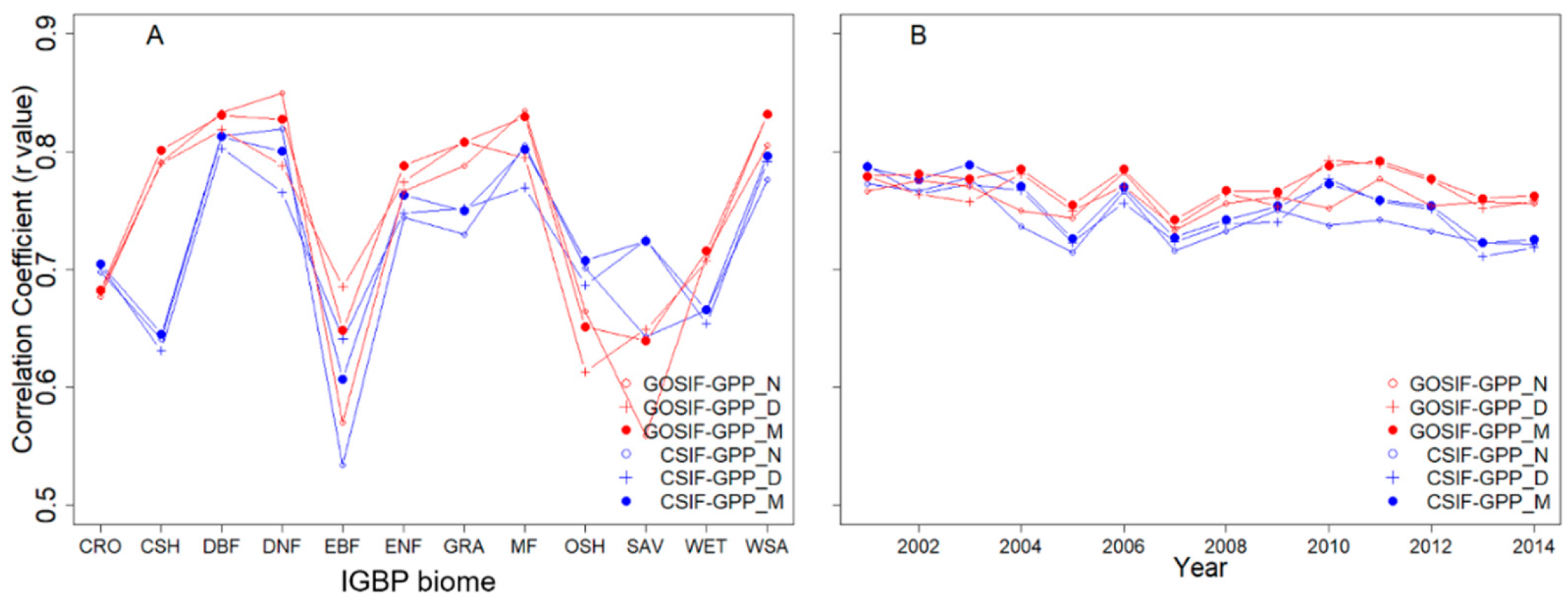
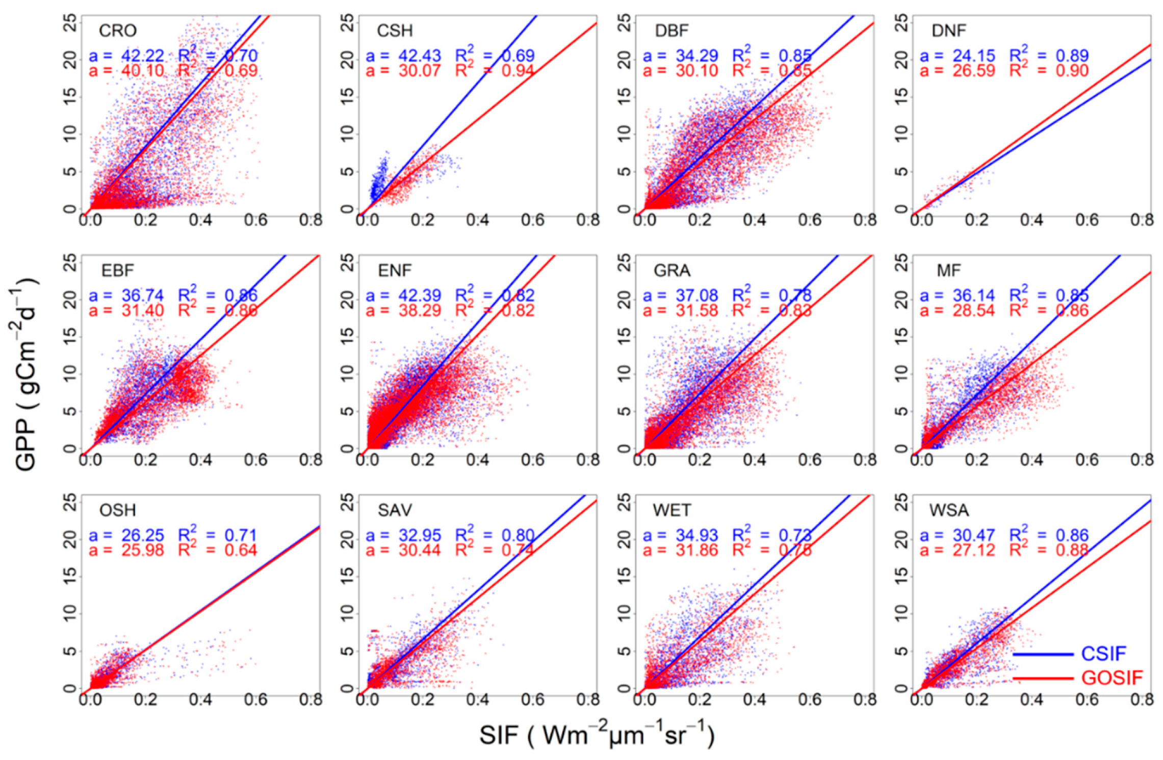
3.1. Correlation between SIFc and GPP

SIFc (both CSIF and GOSIF) showed significant positive correlations with GPP (GPP_D, GPP_N, and GPP_M) worldwide across all the 12 biome types and available years (from 2001 to 2014) (Figure 2). Among biomes, the highest GPP-SIFc correlation was manifested in DBF, and the lowest was in EBF (Figure 2A). The correlations between GOSIF and GPP (i.e., GPP_D, GPP_N, and GPP_M) were higher than those from CSIF in general. However, the r values for GOSIF-GPP were lower than those for CSIF for OSH and SAV biomes (Figure 2A). Strong positive correlations were also observed between SIFc and GPP across all 14 years (r > 0.71, p < 0.001; Figure 2B). Among all the SIFc-GPP correlation coefficients, those of SIFc-GPP_M were the highest: concentrated at 0.76 ± 0.01 and 0.77 ± 0.00 for CSIF and GOSIF, respectively, across 14 years (Figure 2B).

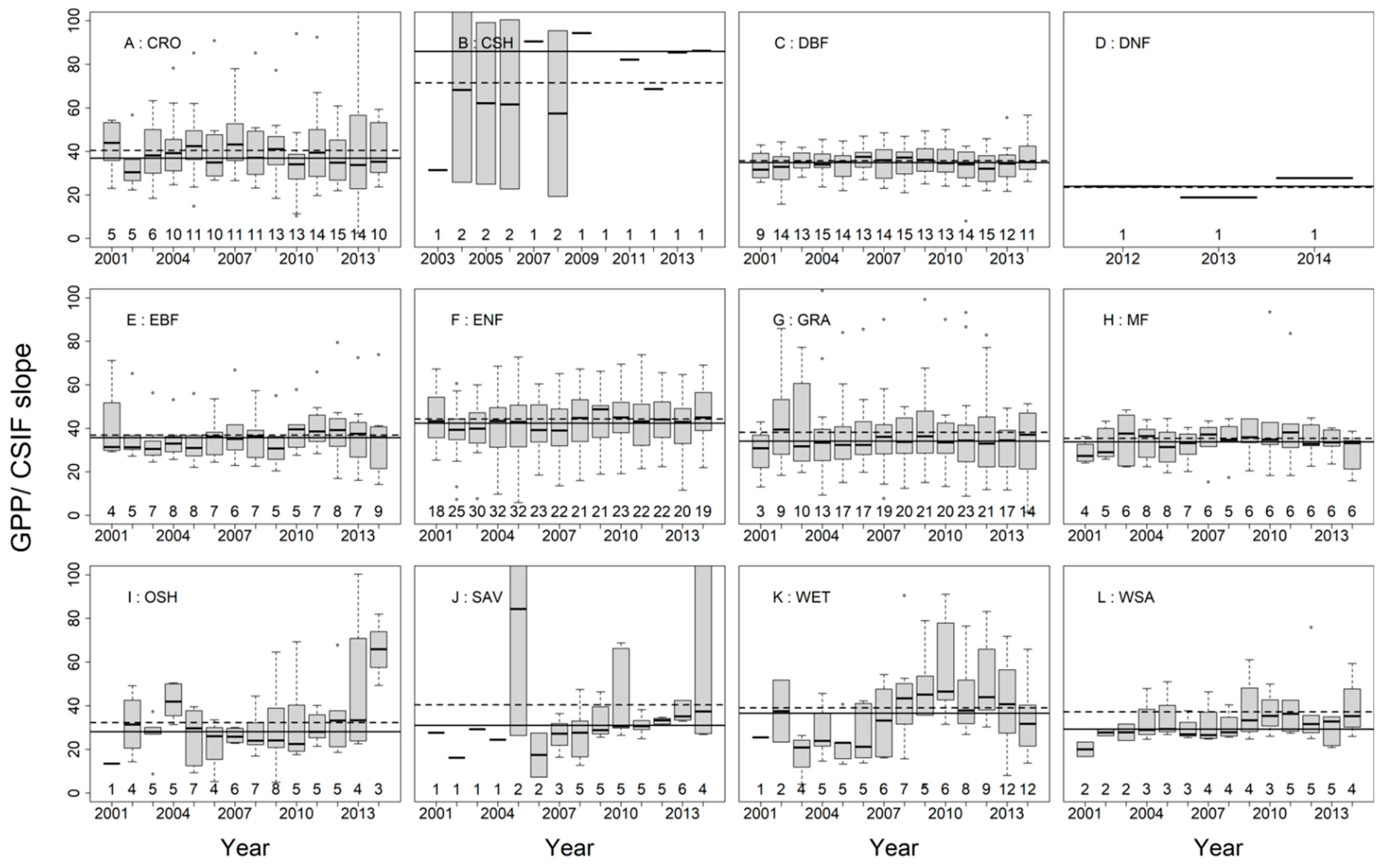
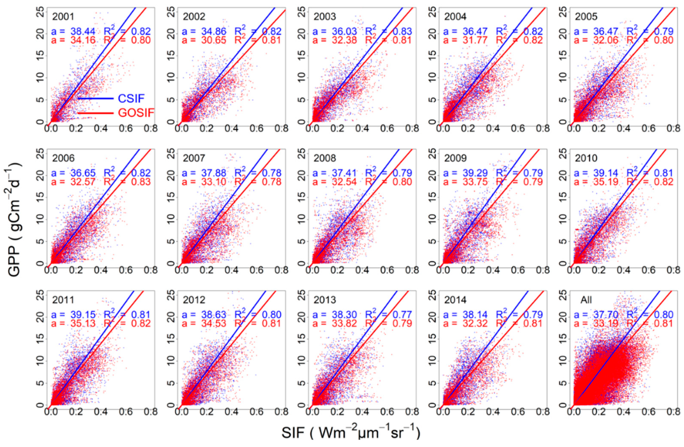
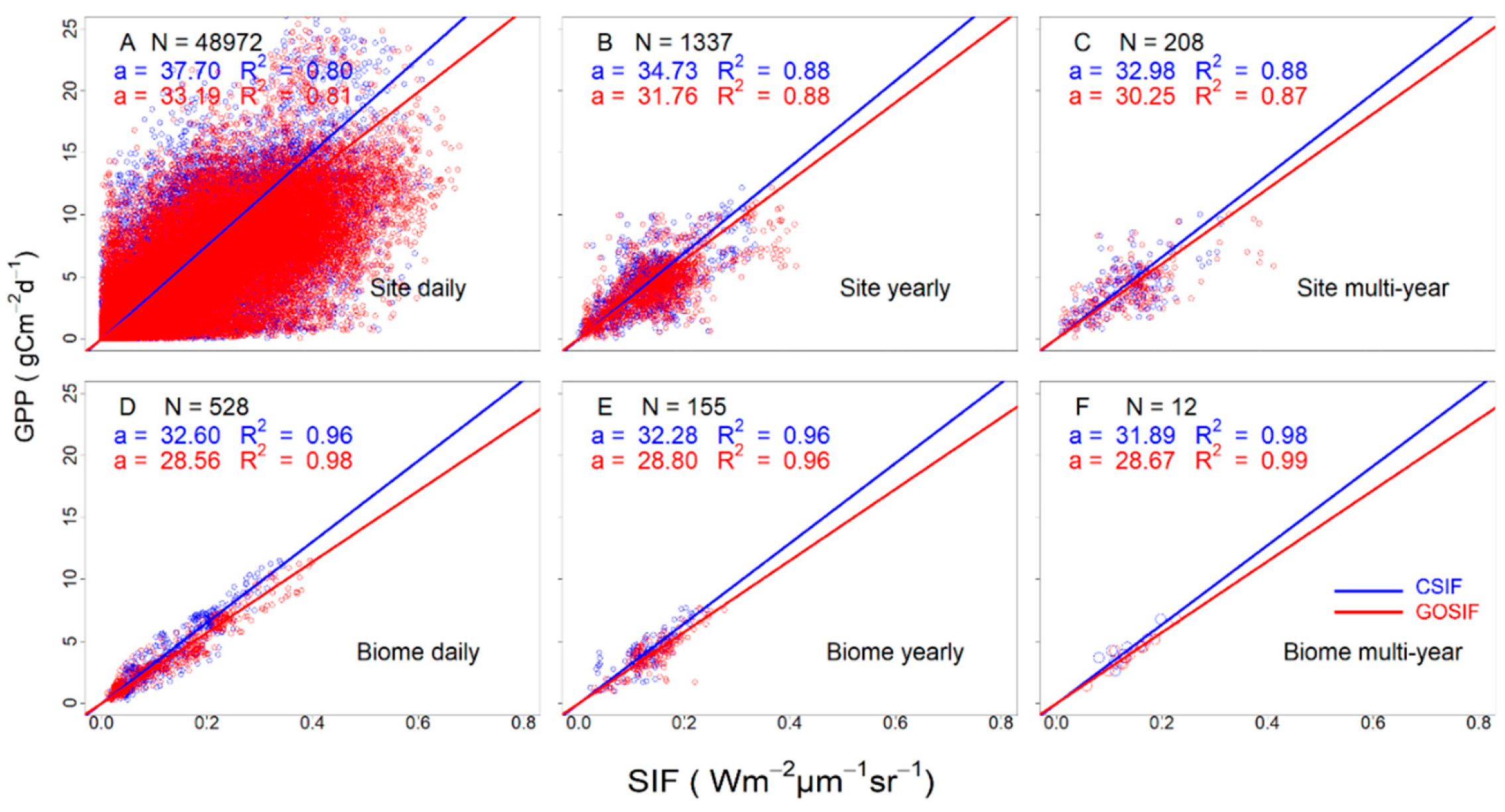
3.2. SIFc–GPP Relationship across Sites, Biomes, and Years

Figure 3 showed the distributions of GPP/SIFc slopes in individual biomes at site-multi-yearly (A and B) and site-yearly (C and D) levels. GPP/SIFc slopes varied greatly across sites and biomes. The CSIF–GPP relationships at the site-multi-yearly scale (Figure 3A) indicated that CSH had the largest inter-site variability with the biggest interquartile ranges (the height of the boxes). In addition, there were significant differences in GPP/CSIF slopes between ENF and several other biomes (i.e., DBF, EBF, GRA and OSH) (p < 0.001), and no significant difference was found among all other biome pairs (p > 0.05). Although the GOSIF–GPP relationships at the site-multi-yearly scale (Figure 3B) look similar to the GOSIF–GPP relationships (Figure 3A), there were substantial differences. First, the GOSIF–GPP inter-site variabilities were smaller than those of GOSIF-GPP in most biomes. Second, with less inter-site variability, the GOSIF-GPP data showed that the number of biomes significantly different from ENF was one more than the CSIF–GPP data (ENF vs. MF) and the significance level (p value) generally increased as well. In addition to these differences, it is important to notice that there was still no significant difference between any non-ENF biome pairs according to GOSIF-GPP (p > 0.05), consistent with CSIF–GPP. The SIFc–GPP relationships at the site-yearly scale (Figure 3C,D), as expected, showed larger variability than those at the site-multi-yearly scale. The ENF biome showed significant differences with all other biomes (p < 0.001), except for the CSH biome with GPP/CSIF slopes (p > 0.05) (Figure 3C,D). However, there were no significant differences of the SIFc–GPP relationship between OSH and DNF biome with other biomes at site-multi-yearly scale (p > 0.05), although the slopes from OSH and DNF are lower than others (Figure 3A,B).
Temporal variability of site-level GPP/CSIF slopes remained relative stable for most biomes except for a few biomes with very limited number of flux towers (i.e., CSH, OSH, SAV, and WET) (Figure 4). Medians of slopes were more similar than means in different variants. The interannual variability of forest biomes were in general the smallest, followed by grassland and cropland. It is interesting to see that the interannual variability of forest, grassland, and cropland biomes remained relatively stable, not affected by the increase of number of flux towers over time in general. In contrast, other biomes differed as the number of sites were small and the number of towers in normal operation fluctuated across years, which led to large interannual variability in the slopes within each of these biomes.
Compared with the GPP/CSIF slopes, the temporal variabilities of the GPP/GOSIF slopes were smaller for most biomes (Figure 5). The reduction of variability was most in those biomes that showed large interannual variabilities in the GPP/CSIF slopes (i.e., CSH, OSH and SAV). The site-variability of wetland (WET) biome expanded greatly from 2009 to 2011 compared with surrounding years and those of GPP/CSIF, and the variability of the grassland (GRA) biome also increased in 2002 and 2003. The enlarged variabilities were probably caused by underestimated GOSIF at a few flux sites in these two biomes in the given years as the median slope was higher than the median and lower than the mean from all years (Figure 5).
Averaging all SIFc and GPP together by biome and ignoring the inter-site differences, strong linear relationships between GPP and SIFc were found consistently across the 12 biomes (Figure 6) and 14 years (Figure 7). Although the SIFc–GPP relationship varied among sites (see Figure 3), the SIFc–GPP relationships at the biome scale were strongly linear (p < 0.001) for both CSIF and GOSIF. However, the large dispersion of the data points also suggests the large temporal (across years) and spatial (across sites) variability (see Figure 3, Figure 4 and Figure 5). For example, the diverging relationship found in CSH was caused by the low CSIF values at the IT.Noe site (Figure S3 and Figure 6).
The linear SIFc–GPP relationships were SIFc dataset-dependent (Figure 6 and Figure 7). The GPP/CSIF slopes were generally higher than GPP/GOSIF slopes for all biomes except DNF (Figure 6). Similar differences existed between GPP/CSIF slopes and GPP/GOSIF slopes for all 14 years (Figure 7). The GPP/CSIF slopes ranged from 34.86 (R2 = 0.82, p < 0.001) to 39.29 (R2 = 0.79, p < 0.001) across 14 years with a mean value of 37.64 ± 0.32, and the value of R2 ranged from 0.77 to 0.83. In contrast, the GPP/GOSIF slopes ranged from 30.65 (R2 = 0.81, p < 0.001) to 35.19 (R2 = 0.82, p < 0.001), with a mean value of 33.14 ± 0.32, and the value of R2 ranged from 0.78 to 0.83. It should be noticed that there were significant differences between CSIF and GOSIF products across all 12 biomes except CSH (Figures S4 and S7) as well as across all 14 years (Figure S5).

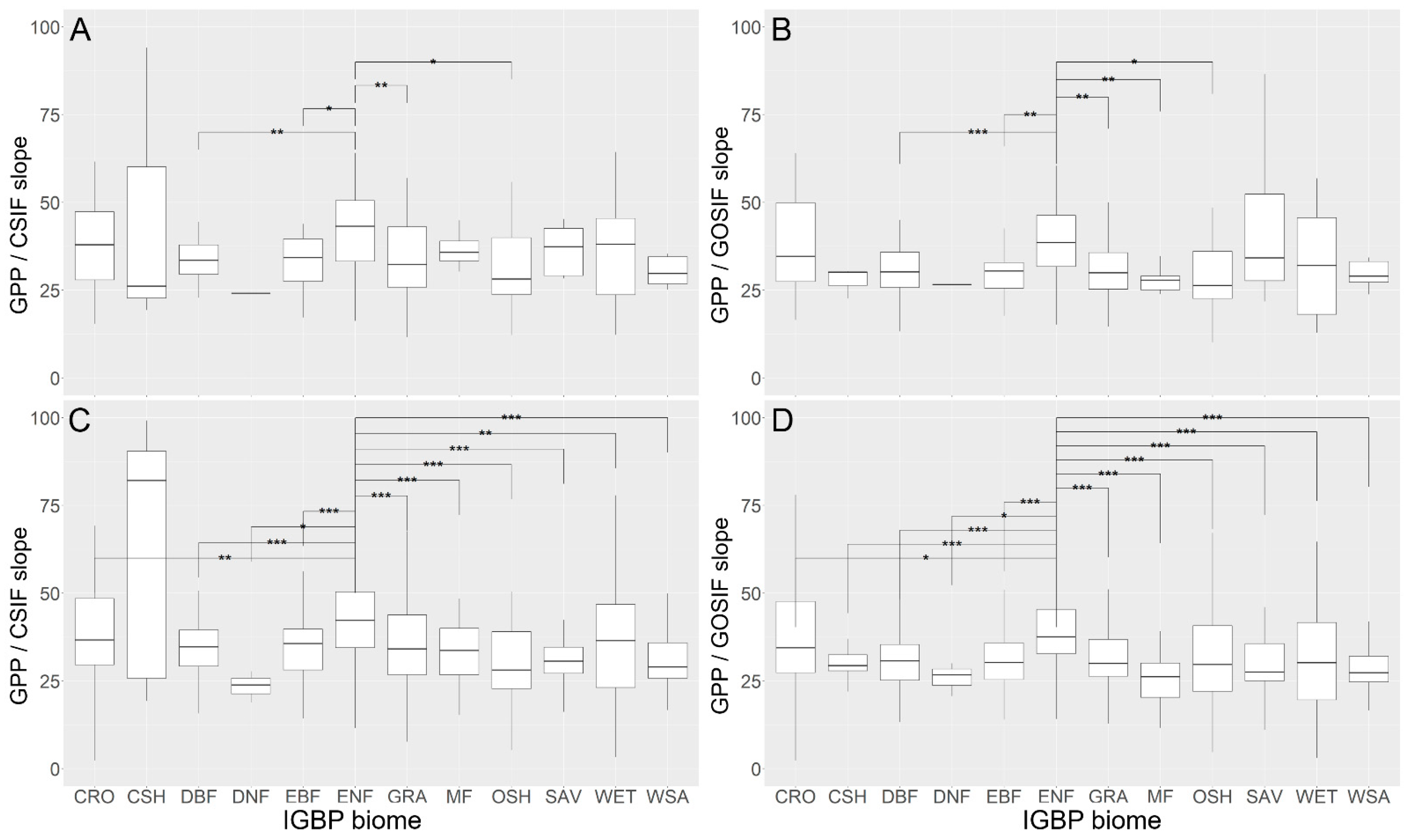
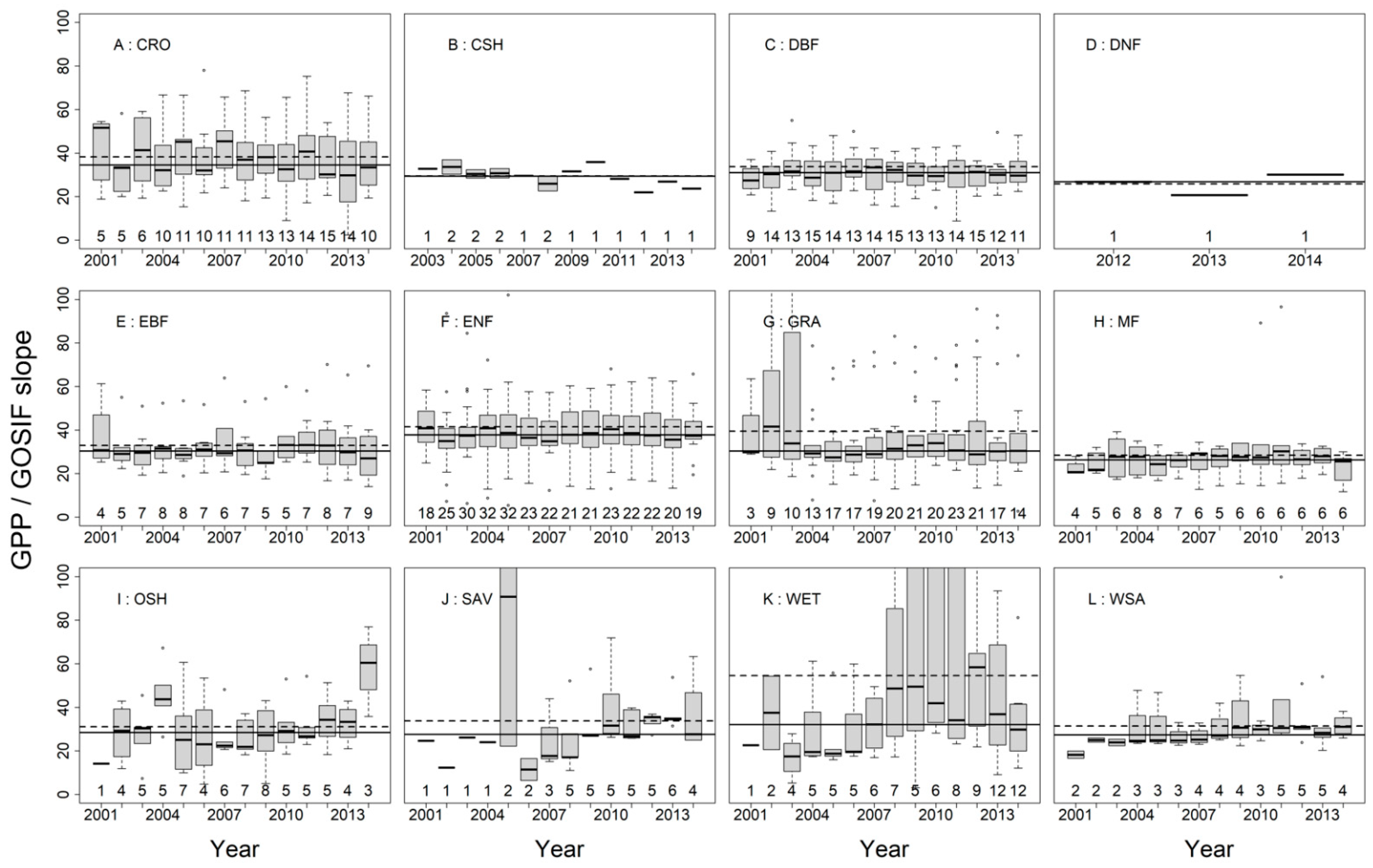
3.3. Variation of the Linear SIFc–GPP Relationship across Spatiotemporal Scales

The robustness of linear SIFc–GPP relationship increased with spatiotemporal upscaling generally (i.e., site-daily, site-yearly, site-multi-yearly, biome-daily, biome-yearly, and biome-multi-yearly scale) (Figure 8). From site to biome level, the R2 values increased while slopes of the linear SIFc–GPP relationship significantly decreased regardless of the time scale. For example, at a daily scale, the R2 value of CSIF–GPP relationship increased from 0.80 to 0.96 from site to biome level, and the corresponding slope decreased from 37.70 to 32.60. Similar changes of R2 values and slopes of linear CSIF–GPP relationship can also be found at yearly and multi-yearly time scales (Figure 8).
The change of R2 values and slopes of the linear SIFc–GPP relationship with the time scale varied with the spatial scale. For example, at the site level, the R2 values of the linear CSIF–GPP relationship increased from daily (slope = 37.70, R2 = 0.80) to yearly (slope = 34.73, R2 = 0.88) scale, but did not increase to multi-yearly (slope = 32.98, R2 = 0.88) scale (Figure 8). Similarly, the R2 values and slopes of linear CSIF–GPP relationship had little changes with the temporal scale at the biome level (daily: slope = 32.60, R2 = 0.96; yearly: slope = 32.28, R2 = 0.96; multi-yearly: slope = 31.89, R2 = 0.98) (Figure 8).

4. Discussion

4.1. Dataset Dependence of the SIFc–GPP Relationship

The linear SIFc–GPP relationship, forced to go through the original point developed from GPP and two contiguous SIFc datasets, is SIFc dataset-dependent (Figure 2). This SIFc dependency can be explained by the fact that GOSIF is generally higher in value than CSIF across biomes and years (Figures S3 and S4). The stronger SIFc–GPP relationship derived from GOSIF compared to that from CSIF was consistent with previous studies [31]. Zhang and Joiner [29] found that the R2 value of the linear relationship between GPP derived from 40 EC flux towers and CSIF ranges from 0.01 to 0.93, with a median value of 0.64. Moreover, Li and Xiao [31] reported a higher linear relationship between GOSIF and flux GPP (R2 = 0.73, p < 0.001) based on the GPP from 91 EC flux towers. However, GOSIF did not always perform better than CSIF in some years and some places (Figure 4 and Figure 5), which might be influenced by the meteorological conditions input. On the other hand, as the differences existing between both SIFc datasets should include variability ranges, systematical bias between different SIFc datasets would lead to different offsets for the linear relationship. Hence, further efforts in improving the SIFc–GPP relationship must reconcile differences from different SIFc datasets and further understand their implications [29,30,31].

4.2. Variability of the SIFc–GPP Relationship

Our results show that the linear SIFc–GPP relationship is significantly affected by the spatial and temporal scales (Figure 8). SIFc–GPP shows the strongest linear relationship at the coarsest scales (i.e., biome-multi-yearly). The R2 value of the linear SIFc–GPP relationship increased with spatial upscaling from site to biome at all temporal scales (i.e., daily, yearly, and multi-yearly). In contrast, the R2 value did not necessarily increase with temporal upscaling at different spatial scales (i.e., site and biome). This suggests that SIFc (both CSIF and GOSIF) is not effective in capturing temporal variabilities of GPP, particularly the inter-annual variability. Overall, the reconstructed SIFc performs well in tracking long-term biome-wide GPP (Figure 8F), consistent with other studies [9]. The reduced ability of SIFc in capturing the short-term changes of GPP might largely be attributed to the errors in SIFc and GPP products, as well as the footprint mismatch between SIFc and GPP, especially at finer resolutions and during the reconstruction period (from 2001 to 2014) [29,31].
It should be noticed that, despite moderate to strong R2 values, there was considerable dispersion in the comparisons of CSIF/GOSIF and GPP at both site and biome levels (Figure 3 and Figure S6). The scattered distribution might be caused by SIFc and flux_GPP data quality as well as the non-universality of the linear GPP-SIFc relationship [44,45], particularly at CRO and DBF biomes (Figures S3 and S6). For example, SIFc-GPP points scattered around the linear regression lines widely at the DE.Geb site (CRO biome) (Figure S6) while the aggregated annual change of flux_GPP synchronized well with those of SIFc in addition to many scattered points caused by interannual variability (Figure S5), suggesting interannual variability of cropping practices (e.g., rotation of crops, fallow, and fertilization) may contribute substantially to the pronounced scattering of points around the regression lines in Figure S6. On the other hand, there were clearly two clusters at the IT.Noe site (CSH biome), which signifies major difference between CSIF and GOSIF there. Clearly, future efforts are required to investigate the variability in the SIF–GPP relationship systematically to answer a suite of important questions: where/when does a linear SIF–GPP relationship break down? Where/when does it change in slope and why?
Li and Xiao [21] reported that C4-dominated grasslands and crops, albeit only two C4 sites, had a significantly higher slope than C3-dominated grasslands and crops (29.42 vs. 20.98, p < 0.001). Moreover, Wood and Griffis [22] found a linear SIF–GPP relationship that is sensitive to crop type (corn vs. soybean) as well. However, our results suggested that there was no significant difference (p > 0.05) in the slopes between C4 (n = 3) and C3 (n = 8) crops at a site-multi-yearly scale, respectively, for CSIF (C4 vs. C3: 42.71 ± 1.33 (mean ± SE) vs. 38.87 ± 5.38) and for GOSIF (C4 vs. C3: 38.70 ± 3.48 vs. 40.32 ± 6.11). The difference between our study and Li and Xiao [21] may be due to the limited number of C4 crop sites and the different approaches used for analysis. We compared the difference in the means of the slopes from individual C3 and C4 sites, while Li and Xiao [21] compared the difference in the overall slopes of the C3 and C4 crops after pooling SIF and GPP data from all C3 and C4 sites. Apparently, further research is needed to understand the differences in the SIF–GPP relationships for C3/C4 plants with more C4 sites.
The number of EC flux towers is not balanced among the biomes, and some biomes only include one or a few sites. This leads to large uncertainties in the linear GPP/SIFc slopes in some biomes (e.g., CSH, OSH, and WET). For example, the GPP/CSIF slopes of OSH and DNF were lower than other biomes; there are clearly two clusters of data captured within CSH (Figure 3). The main reason may be the limited GPP data at OSH (72 site-yearly) and DNF (3 site-yearly) biomes. Thus, increasing the number of EC flux towers, particularly in some underrepresented biomes (e.g., OSH and DNF), is necessary to make our global analysis more representative and robust to support GPP modeling using SIF.

4.3. A Generic Two-Slope Scheme SIFc–GPP Relationship

Our study found that at site-multi-yearly scale there was no significant difference between any biome pairs in GPP/SIFc slopes except a few pairs between ENF and others (Figure 3). Specifically, GPP/SIFc slopes in ENF biome were significantly higher than those in four biomes (DBF, EBF, GRA, and OSH) according to CSIF or five biomes (DBF, EBF, GRA, OSH, and MF) according to GOSIF, and the slopes between any other non-ENF biome pairs were not significantly different. To summarize these findings, we, therefore, propose a two-slope scheme to differentiate ENF from non-ENF and synopsize the GPP/SIFc slope variability across all biomes and years. It should be noted that the two-slope scheme is SIFc dataset-specific (Table 1), resulting from the systematic differences between these two SIFc datasets.
To sift the statistics (mean or median slope) building the two-slope scheme, we compared the SIFc-derived GPP with flux tower GPP. It can be seen that the two-slope scheme derived from median values (median PB were 7.14% and 11.06% for GOSIF and CSIF, respectively) outperformed the one from the mean values (median PB were 31.65% and 20.67% for GOSIF and CSIF, respectively) in estimating GPP across all EC towers (Figure 9, Figure S8 and S9); probably, the median-based scheme effectively avoided the impacts of slope outliers. Thus, we used the median values of slopes to develop the two-slope scheme in this study. The median slopes for the GPP/CSIF were 43.21 (13.39) and 34.36 (11.66) with corresponding mean ± SE as 42.75 ± 2.04 and 38.41 ± 1.74, respectively, for ENF and other biomes (Table 1), resulting in the following two-slope scheme for converting CSIF into GPP:
GPP = { 43.21 × SIF ,         ENF     biome         34.36 × SIF ,         other   biomes
The median slopes for the GPP/GOSIF were 38.61 (10.65) and 30.39 (9.65) with corresponding mean ± SE as 40.36 ± 2.28 and 39.09 ± 3.02, respectively, for ENF and other biomes, and the corresponding two-slope scheme was:
GPP = { 38.61 × SIF ,             ENF   biome         30.39 × SIF ,           other   biomes
The two-slope scheme provides a very convenient and effective tool for converting SIFc to GPP and monitoring GPP dynamics in time and space as it is almost land cover-independent (only the distribution of ENF needs to be identified). The significantly higher slopes for the ENF biome in the two-slope scheme are intriguing and deserve further study. This phenomenon is in line with the observations reported by Gamon and Huemmrich [46] and Zhang and Joiner [29], who pointed out that the lower SIF (and therefore, higher GPP/SIFc slope) for ENF is mainly caused by a stronger canopy reabsorption and/or scattering of SIF for the needle leaf forest, and the core mechanism is the high dependency between SIF and APAR, chlorophyll content [47], and photosynthetic light-use efficiency [48]. However, it is still a great challenge to measure (in field), observe (from satellite), and model (mechanism-based) photosynthesis in boreal forests, especially for the ENF biome [48,49]. More in-depth research is still needed to expand our understanding of the effects of needle leaf clumping index [50]), leaf chlorophyll content [51], and chlorophyll/carotenoid index [46] on plant photosynthesis (especially for SIF as an agents) from canopy to global scale [9].
The coefficients for the two SIF datasets are different from each other (Equations (1) and (2)). It can be explained by the fact that GOSIF is generally higher in value than CSIF across biomes and years (Figures S4 and S5), which can be traced back to their reconstruction methods and the uncertainty of the SIFc products. GOSIF, generated from discrete OCO-2 SIF soundings, EVI, and land cover type data from MODIS and meteorological reanalysis data, had an RMSE of only 0.07 W m−2 µm−1 sr−1 [31]. In contrast, CSIF, generated using a machine learning approach (trained by discrete OCO-2 SIF soundings and MODIS surface reflectance), had an RMSE of 0.18 W m−2 μm−1 sr−1 [29], more than double that of GOSIF.
Previous studies have highlighted that the linear SIF–GPP relationship is either biome-dependent [22,26] or ecosystem-specific (e.g., Sun and C. Frankenberg [2]). To our knowledge, none of them has really examined the discriminatory power of their datasets on the observed differences of SIF–GPP relationship across ecosystems or biomes. In other words, previous studies often studied the uniqueness of the SIF–GPP relationships, and none addressed their commonality or the discriminatory power of their datasets across biomes. Our two-slope scheme represents a major step forward in this direction. In addition, it provides a practicable method for estimating GPP from SIFc with a greatly reduced need on land cover specificity, which should benefit the reduction of GPP uncertainty from land cover classification. This general scheme may have reconciled the differences among previous studies that were either restricted to small regions [52], had too few flux towers and/or biomes [21], or had low spatiotemporal resolutions [28].

4.4. Potential Caveats and Uncertainties

Landscape heterogeneity and inconsistency between the flux-tower footprint and SIFc pixel should have contributed to the uncertainty of our results [53]. We acknowledge that the landscape heterogeneity at the EC flux towers is an important obstacle to analyzing the SIF–GPP relationship. Although we have visually checked landscape conditions around all EC-flux tower sites using Google Earth images, and removed four flux towers from our analysis, a more robust approach to address the issue would be using a footprint model to obtain the footprints of all the sites. Our manual examination approach resulted in 208 sites, which was different from that of Zhang and Joiner [29], who selected only 40 sites using an automated NDVI-based approach. Our results, therefore, might have higher uncertainties than Zhang and Joiner [29], but at the same time, encompassed more spatial variability of sites globally, which might enhance the representativeness of our results. The results derived from this new paradigm should be better suited to real-world applications than those derived from the conventional approach because of the ubiquity of heterogeneous landscapes [53]. Furthermore, applying the results from conventional analysis that only cover ‘homogenous’ landscapes to the real world would result in unknown amount of uncertainty. The latter is demonstrated by the good performance of the median-based two-slope scheme at many flux-tower sites and biomes (Figure 9). Retrospectively, our two-slope scheme suggests that the impact of landscape heterogeneity and inconsistency between the flux tower footprint and SIFc pixel might not as severe as we previously thought.
In addition, for CRO and GRA biomes, the site selection is particularly important, as the flux towers at these biomes are of a height of 2–6 m and the footprint areas are similar when visualized with the SIFc pixel. On top of that, the GPP from these sites very much depend on the crop and management practice (e.g., rotation of crops, fallow, grazing, and fertilization), which can change every few hundred meters, thereby making the satellite-ground comparison challenging.
Whether the regression method used in this study works well also introduced uncertainty. Just from the mathematical view, one of the fundamental problems of forcing the intercept to zero is getting a much higher R2 (Figure 8), which will lead to a large portion of bias in the results, especially at a daily scale [2]. Conversely, at the point of vegetation physiology, the zero-intercept logic provides a unique perspective for the SIFc–GPP relationship analysis. Xiao and Li [54] reported that the low daily SIF/GPP measurements are not available in some areas/biomes, such as EBF. In such occasions, the application of our zero-intercept logic makes more sense, which may have greater predictability under unseen conditions (e.g., low SIF/GPP). As this study focused on the comparison of GPP/SIFc slopes across different biomes, we finally applied the zero-intercept method rather than the free intercept. Nevertheless, some free intercept regression model would provide more information about the SIFc–GPP relationship [43].

5. Conclusions

Our work is a global analysis investigating the relationship between SIFc and GPP at various spatial and temporal scales, which expands previous research on this topic, particularly in the following two areas. First, we used all GPP data in the FLUXNET2015 collection and two global SIFc products for the analysis, providing the most comprehensive coverage so far (208 flux towers and the longest study period from 2001 to 2014) to explore the SIFc–GPP relationship. Second, we used Major Axis regression to account for uncertainties in both SIFc and GPP estimates in the analysis of the SIFc–GPP relationship, which produced higher GPP/SIFc slopes than OLS. Our research expands several pioneering works which have reported the relationship between OCO-2 SIF and tower GPP at individual sites and a few biomes. We propose a two-slope scheme to differentiate ENF from the non-ENF biome and synopsize the GPP/SIFc slope variability across biomes and years. The relative biases were 7.14% and 11.06% in the estimated cumulative GPP across all EC towers, respectively, for GOSIF and CSIF, using the two-slope scheme. Nevertheless, our results suggested some major issues related to the SIFc–GPP relationship, including dataset dependency of the SIFc–GPP relationship, variability of the SIFc–GPP relationship across spatial and temporal scales, and a two-slope scheme that was distilled from the SIFc–GPP relationships across biomes. Thus, we call for more research on these abovementioned issues, and offer a few thoughts on the caveats and uncertainties of our research, as well as future research directions.

Supplementary Materials

Author Contributions

Conceptualization, S.L.; methodology, S.L. and H.G.; writing—original draft preparation, H.G.; writing—review and editing, S.L., W.L., A.R.S., W.Y., Z.W. (Zhao Wang), X.P., R.V., L.X., Q.L., Y.F., M.M., T.P., J.L., Z.W. (Zhenming Wu), G.Z. and H.G.; supervision, S.L.; funding acquisition, S.L. All authors have read and agreed to the published version of the manuscript.

Funding

This research was funded by the National Natural Science Foundation of China (Grant No. 41971152); and the Hunan Innovative Talent Program (Grant No. 2019RS1062) to S Liu.

Acknowledgments

This work used EC flux data acquired and shared by the FLUXNET community, including the following networks: AmeriFlux, AfriFlux, AsiaFlux, CarboAfrica, CarboEuropeIP, CarboItaly, CarboMont, ChinaFlux, Fluxnet-Canada, GreenGrass, ICOS, KoFlux, LBA, NECC, OzFlux-TERN, TCOS-Siberia, and USCCC. The ERA-Interim reanalysis data are provided by ECMWF and processed by LSCE. The FLUXNET EC flux data processing and harmonization were carried out by the European Fluxes Database Cluster, AmeriFlux Management Project, and Fluxdata project of FLUXNET, with the support of CDIAC and the ICOS Ecosystem Thematic Center, and the OzFlux, ChinaFlux, and AsiaFlux offices. The CSIF dataset is provided by Yao Zhang, and the GOSIF dataset is provided by Xing Li and Jingfeng Xiao. We thank the anonymous reviewers for their valuable comments.

Conflicts of Interest

We declare that we have no financial and personal relationships with other people or organizations that can inappropriately influence our work, there are no professional or other personal interests of any nature or kind in any product, service, and/or company that could be construed as influencing the position presented in, or the review of, the manuscript entitled “Global analysis of the relationship between reconstructed solar induced chlorophyll fluorescence (SIF) and GPP.”

References

  1. Beer, C.; Reichstein, M.; Tomelleri, E.; Ciais, P.; Jung, M.; Carvalhais, N.; Rödenbeck, C.; Arain, M.A.; Baldocchi, D.; Bonan, G.B.; et al. Terrestrial gross carbon dioxide uptake: Global distribution and covariation with climate. Science 2010, 329, 834–838. [Google Scholar] [CrossRef] [Green Version]
  2. Sun, Y.; Frankenberg, C.; Wood, J.D.; Schimel, D.S.; Jung, M.; Guanter, L.; Drewry, D.T.; Verma, M.; Porcar-Castell, A.; Griffis, T.J.; et al. OCO-2 advances photosynthesis observation from space via solar-induced chlorophyll fluorescence. Science 2017, 358, eaam5747. [Google Scholar] [CrossRef] [PubMed] [Green Version]
  3. Frankenberg, C.; Fisher, J.; Worden, J.; Badgley, G.; Saatchi, S.S.; Lee, J.-E.; Toon, G.C.; Butz, A.; Jung, M.; Kuze, A.; et al. New global observations of the terrestrial carbon cycle from GOSAT: Patterns of plant fluorescence with gross primary productivity. Geophys. Res. Lett. 2011, 38. [Google Scholar] [CrossRef] [Green Version]
  4. Wei, X.; Wang, X.; Wei, W.; Wan, W. Use of Sun-Induced Chlorophyll Fluorescence Obtained by OCO-2 and GOME-2 for GPP Estimates of the Heihe River Basin, China. Remote Sens. 2018, 10, 2039. [Google Scholar] [CrossRef] [Green Version]
  5. Eldering, A.; Wennberg, P.O.; Crisp, D.; Schimel, D.S.; Gunson, M.R.; Chatterjee, A.; Liu, J.; Schwandner, F.M.; Sun, Y.; O’Dell, C.W.; et al. The Orbiting Carbon Observatory-2 early science investigations of regional carbon dioxide fluxes. Science 2017, 358, eaam5745. [Google Scholar] [CrossRef] [Green Version]
  6. Baker, N.R. Chlorophyll fluorescence: A probe of photosynthesis in vivo. Annu. Rev. Plant Biol. 2008, 59, 89–113. [Google Scholar] [CrossRef] [PubMed] [Green Version]
  7. Zhang, L.; Qiao, N.; Huang, C.; Wang, S. Monitoring Drought Effects on Vegetation Productivity Using Satellite Solar-Induced Chlorophyll Fluorescence. Remote Sens. 2019, 11, 378. [Google Scholar] [CrossRef] [Green Version]
  8. Magney, T.S.; Bowling, D.R.; Logan, B.; Grossmann, K.; Stutz, J.; Blanken, P.D.; Burns, S.P.; Cheng, R.; Garcia, M.A.; Köhler, P.; et al. Mechanistic evidence for tracking the seasonality of photosynthesis with solar-induced fluorescence. Proc. Natl. Acad. Sci. USA 2019, 116, 11640–11645. [Google Scholar] [CrossRef] [PubMed] [Green Version]
  9. Ryu, Y.; Berry, J.A.; Baldocchi, D.D. What is global photosynthesis? History, uncertainties and opportunities. Remote Sens. Environ. 2019, 223, 95–114. [Google Scholar] [CrossRef]
  10. Yokota, T.; Yoshida, Y.; Eguchi, N.; Ota, Y.; Tanaka, T.; Watanabe, H.; Maksyutov, S. Global Concentrations of CO2 and CH4 Retrieved from GOSAT: First Preliminary Results. SOLA 2009, 5, 160–163. [Google Scholar] [CrossRef] [Green Version]
  11. Joiner, J.; Yoshida, Y.; Vasilkov, A.P.; Middleton, E.M.; Campbell, P.K.E.; Kuze, A.; Corp, L.A. Filling-in of near-infrared solar lines by terrestrial fluorescence and other geophysical effects: Simulations and space-based observations from SCIAMACHY and GOSAT. Atmos. Meas. Tech. 2012, 5, 809–829. [Google Scholar] [CrossRef] [Green Version]
  12. Joiner, J.; Guanter, L.; Lindstrot, R.; Voigt, M.; Vasilkov, A.P.; Middleton, E.M.; Huemmrich, K.F.; Yoshida, Y.; Frankenberg, C. Global monitoring of terrestrial chlorophyll fluorescence from moderate-spectral-resolution near-infrared satellite measurements: Methodology, simulations, and application to GOME-2. Atmos. Meas. Tech. 2013, 6, 2803–2823. [Google Scholar] [CrossRef] [Green Version]
  13. Köhler, P.; Guanter, L.; Joiner, J. A linear method for the retrieval of sun-induced chlorophyll fluorescence from GOME-2 and SCIAMACHY data. Atmos. Meas. Tech. 2015, 8, 2589–2608. [Google Scholar] [CrossRef] [Green Version]
  14. Wen, J.; Köhler, P.; Duveiller, G.; Parazoo, N.; Magney, T.; Hooker, G.; Yu, L.; Chang, C.; Sun, Y. A framework for harmonizing multiple satellite instruments to generate a long-term global high spatial-resolution solar-induced chlorophyll fluorescence (SIF). Remote Sens. Environ. 2020, 239, 111644. [Google Scholar] [CrossRef]
  15. Du, S.; Liu, L.; Liu, X.; Zhang, X.; Zhang, X.; Bi, Y.; Zhang, L. Retrieval of global terrestrial solar-induced chlorophyll fluorescence from TanSat satellite. Sci. Bull. 2018, 63, 1502–1512. [Google Scholar] [CrossRef] [Green Version]
  16. Köhler, P.; Frankenberg, C.; Magney, T.S.; Guanter, L.; Joiner, J.; Landgraf, J. Global Retrievals of Solar-Induced Chlorophyll Fluorescence With TROPOMI: First Results and Intersensor Comparison to OCO-2. Geophys. Res. Lett. 2018, 45, 10456–10463. [Google Scholar] [CrossRef] [Green Version]
  17. Frankenberg, C.; O’Dell, C.; Berry, J.; Guanter, L.; Joiner, J.; Köhler, P.; Pollock, R.; Taylor, T.E. Prospects for chlorophyll fluorescence remote sensing from the Orbiting Carbon Observatory-2. Remote Sens. Environ. 2014, 147, 1–12. [Google Scholar] [CrossRef] [Green Version]
  18. Zuromski, L.M.; Bowling, D.R.; Köhler, P.; Frankenberg, C.; Goulden, M.L.; Blanken, P.D.; Lin, J.C. Solar-Induced Fluorescence Detects Interannual Variation in Gross Primary Production of Coniferous Forests in the Western United States. Geophys. Res. Lett. 2018, 45, 7184–7193. [Google Scholar] [CrossRef]
  19. Guanter, L.; Frankenberg, C.; Dudhia, A.; Lewis, P.; Gómez-Dans, J.; Kuze, A.; Suto, H.; Grainger, R. Retrieval and global assessment of terrestrial chlorophyll fluorescence from GOSAT space measurements. Remote Sens. Environ. 2012, 121, 236–251. [Google Scholar] [CrossRef]
  20. Porcar-Castell, A.; Tyystjärvi, E.; Atherton, J.; van der Tol, C.; Flexas, J.; Pfündel, E.E.; Moreno, J.; Frankenberg, C.; Berry, J.A. Linking chlorophyll a fluorescence to photosynthesis for remote sensing applications: Mechanisms and challenges. J. Exp. Bot. 2014, 65, 4065–4095. [Google Scholar] [CrossRef]
  21. Li, X.; Xiao, J.; He, B.; Arain, M.A.; Beringer, J.; Desai, A.R.; Emmel, C.; Hollinger, D.Y.; Krasnova, A.; Mammarella, I.; et al. Solar-induced chlorophyll fluorescence is strongly correlated with terrestrial photosynthesis for a wide variety of biomes: First global analysis based on OCO-2 and flux tower observations. Glob. Chang. Biol. 2018, 24, 3990–4008. [Google Scholar] [CrossRef]
  22. Wood, J.D.; Griffis, T.J.; Baker, J.M.; Frankenberg, C.; Verma, M.; Yuen, K. Multiscale analyses of solar-induced florescence and gross primary production. Geophys. Res. Lett. 2017, 44, 533–541. [Google Scholar] [CrossRef]
  23. Li, X.; Xiao, J.; He, B. Chlorophyll fluorescence observed by OCO-2 is strongly related to gross primary productivity estimated from flux towers in temperate forests. Remote Sens. Environ. 2018, 204, 659–671. [Google Scholar] [CrossRef]
  24. Zhang, Y.; Xiao, X.; Zhang, Y.; Wolf, S.; Zhou, S.; Joiner, J.; Guanterg, L.; Verma, M.; Sun, Y.; Yang, X.; et al. On the relationship between sub-daily instantaneous and daily total gross primary production: Implications for interpreting satellite-based SIF retrievals. Remote Sens. Environ. 2018, 205, 276–289. [Google Scholar] [CrossRef] [Green Version]
  25. Wang, X.; Chen, J.M.; Ju, W. Photochemical reflectance index (PRI) can be used to improve the relationship between gross primary productivity (GPP) and sun-induced chlorophyll fluorescence (SIF). Remote Sens. Environ. 2020, 246, 111888. [Google Scholar] [CrossRef]
  26. Sun, Y.; Frankenberg, C.; Jung, M.; Joanna, J.; Guanter, L.; Kohler, P.; Magney, T.S. Overview of Solar-Induced chlorophyll Fluorescence (SIF) from the Orbiting Carbon Observatory-2: Retrieval, cross-mission comparison, and global monitoring for GPP. Remote Sens. Environ. 2018, 209, 808–823. [Google Scholar] [CrossRef]
  27. Chen, B.; Black, T.A.; Coops, N.C.; Hilker, T.; Trofymow, J.A.; Morgenstern, K. Assessing Tower Flux Footprint Climatology and Scaling Between Remotely Sensed and Eddy Covariance Measurements. BoLMe 2009, 130, 137–167. [Google Scholar] [CrossRef]
  28. Zhang, Y.; Guanter, L.; Berry, J.A.; Van der Tol, C.; Yang, X.; Tang, J.; Zhang, F. Model-based analysis of the relationship between sun-induced chlorophyll fluorescence and gross primary production for remote sensing applications. Remote Sens. Environ. 2016, 187, 145–155. [Google Scholar] [CrossRef] [Green Version]
  29. Zhang, Y.; Joiner, J.; Alemohammad, S.H.; Zhou, S.; Gentine, P. A global spatially contiguous solar-induced fluorescence (CSIF) dataset using neural networks. Biogeosciences 2018, 15, 5779–5800. [Google Scholar] [CrossRef] [Green Version]
  30. Yu, L.; Xiao, X.; Zhang, Y.; Wolf, S.; Zhou, S.; Joiner, J.; Guanter, L.; Verma, M.; Sun, Y. High Resolution Global Contiguous Solar-Induced Chlorophyll Fluorescence (SIF) of Orbiting Carbon Observatory-2 (OCO-2). Geophys. Res. Lett. 2018, 205, 276–289. [Google Scholar]
  31. Li, X.; Xiao, J. A Global, 0.05-Degree Product of Solar-Induced Chlorophyll Fluorescence Derived from OCO-2, MODIS, and Reanalysis Data. Remote Sens. 2019, 11, 517. [Google Scholar] [CrossRef] [Green Version]
  32. Gelaro, R.; McCarty, W.; Suárez, M.J.; Todling, R.; Molod, A.; Takacs, L.; Randles, C.A.; Darmenov, A.; Bosilovich, M.G.; Reichle, R.; et al. The Modern-Era Retrospective Analysis for Research and Applications, Version 2 (MERRA-2). J. Clim. 2017, 30, 5419–5454. [Google Scholar] [CrossRef]
  33. Duveiller, G.; Filipponi, F.; Walther, S.; Köhler, P.; Frankenberg, C.; Guanter, L.; Cescatti, A. A spatially downscaled sun-induced fluorescence global product for enhanced monitoring of vegetation productivity. Earth Syst. Sci. Data 2020, 12, 1101–1116. [Google Scholar] [CrossRef]
  34. Pastorello, G.Z.; Papale, D.; Chu, H.; Trotta, C.; Agarwal, D.A.; Canfora, E.; Baldocchi, D.D.; Torn, M. A New Data Set to Keep a Sharper Eye on Land-Air Exchanges. Eos 2017, 98. [Google Scholar] [CrossRef]
  35. Li, X.; Xiao, J. Mapping Photosynthesis Solely from Solar-Induced Chlorophyll Fluorescence: A Global, Fine-Resolution Dataset of Gross Primary Production Derived from OCO-2. Remote Sens. 2019, 11, 2563. [Google Scholar] [CrossRef] [Green Version]
  36. Reichstein, M.; Falge, E.; Baldocchi, D.; Papale, D.; Aubinet, M.; Berbigier, P.; Bernhofer, C.; Buchmann, N.; Gilmanov, T.; Granier, A.; et al. On the separation of net ecosystem exchange into assimilation and ecosystem respiration: Review and improved algorithm. Glob. Chang. Biol. 2005, 11, 1424–1439. [Google Scholar] [CrossRef]
  37. Zhang, Y.; Xiao, X.; Wu, X.; Zhou, S.; Zhang, G.; Qin, Y.; Dong, J. A global moderate resolution dataset of gross primary production of vegetation for 2000–2016. Sci. Data 2017, 4, 170165. [Google Scholar] [CrossRef] [Green Version]
  38. Friedl, M.A.; McIver, D.K.; Baccini, A.; Gao, F.; Schaaf, C.; Hodges, J.C.F.; Zhang, X.Y.; Muchoney, D.; Strahler, A.H.; Woodcock, C.E.; et al. Global land cover mapping from MODIS: Algorithms and early results. Remote Sens. Environ. 2002, 83, 287–302. [Google Scholar] [CrossRef]
  39. R Core Team. R: A Language and Environment for Statistical Computing; R Foundation for Statistical Computing: Vienna, Austria, 2019. [Google Scholar]
  40. Loveland, T.R.; Reed, B.C.; Brown, J.F.; Ohlen, D.O.; Zhu, Z.; Yang, L.W.M.J.; Merchant, J.W. Development of a global land cover characteristics database and IGBP DISCover from 1 km AVHRR data. Int. J. Remote Sens. 2000, 21, 1303–1330. [Google Scholar] [CrossRef]
  41. Belward, A.S. The IGBP-DIS Global 1 km Land Cover Data Set “DISCover”: Proposal and Implementation Plans: Report of the Land Cover Working Group of IGBP-DIS; IGBP-DIS Office: Alexandria, VA, USA, 1992. [Google Scholar]
  42. Warton, D.I.; Duursma, R.; Falster, D.S.; Taskinen, S. smatr 3—An R package for estimation and inference about allometric lines. Methods Ecol. Evol. 2012, 3, 257–259. [Google Scholar] [CrossRef]
  43. Zhang, Z.; Zhang, Y.; Joiner, J.; Migliavacca, M. Angle matters: Bidirectional effects impact the slope of relationship between gross primary productivity and sun-induced chlorophyll fluorescence from Orbiting Carbon Observatory-2 across biomes. Glob. Chang. Biol. 2018, 24, 5017–5020. [Google Scholar] [CrossRef] [Green Version]
  44. Marrs, J.K.; Reblin, J.S.; Logan, B.A.; Allen, D.W.; Reinmann, A.B.; Bombard, D.M.; Tabachnik, D.; Hutyra, L.R. Solar-Induced Fluorescence Does Not Track Photosynthetic Carbon Assimilation Following Induced Stomatal Closure. Geophys. Res. Lett. 2020, 47, e2020GL087956. [Google Scholar] [CrossRef]
  45. Wang, Z.; Liu, S.; Wang, Y.; Valbuena, R.; Wu, Y.; Kutia, M.; Zheng, Y.; Lu, W.; Zhu, Y.; Zhao, M.; et al. Tighten the Bolts and Nuts on GPP Estimations from Sites to the Globe: An Assessment of Remote Sensing Based LUE Models and Supporting Data Fields. Remote Sens. 2021, 13, 168. [Google Scholar] [CrossRef]
  46. Gamon, J.A.; Huemmrich, K.F.; Wong, C.Y.S.; Ensminger, I.; Garrity, S.; Hollinger, D.Y.; Noormets, A.; Peñuelas, J. A remotely sensed pigment index reveals photosynthetic phenology in evergreen conifers. Proc. Natl. Acad. Sci. USA 2016, 113, 13087–13092. [Google Scholar] [CrossRef] [PubMed] [Green Version]
  47. Louis, J.; Ounis, A.; Ducruet, J.-M.; Evain, S.; Laurila, T.; Thum, T.; Aurela, M.; Wingsle, G.; Alonso, L. Remote sensing of sunlight-induced chlorophyll fluorescence and reflectance of Scots pine in the boreal forest during spring recovery. Remote Sens. Environ. 2005, 96, 37–48. [Google Scholar] [CrossRef] [Green Version]
  48. Walther, S.; Voigt, M.; Thum, T.; Gonsamo, A.; Zhang, Y.; Köhler, P.; Jung, M.; Varlagin, A.; Guanter, L. Satellite chlorophyll fluorescence measurements reveal large-scale decoupling of photosynthesis and greenness dynamics in boreal evergreen forests. Glob. Chang. Biol. 2016, 22, 2979–2996. [Google Scholar] [CrossRef] [PubMed] [Green Version]
  49. Pisek, J.; Chen, J.M.; Nilson, T. Estimation of vegetation clumping index using MODIS BRDF data. Int. J. Remote Sens. 2011, 32, 2645–2657. [Google Scholar] [CrossRef]
  50. He, L.; Liu, J.; Chen, J.M.; Croft, H.; Wang, R.; Sprintsin, M.; Zheng, T.; Ryu, Y.; Pisek, J.; Gonsamo, A.; et al. Inter- and intra-annual variations of clumping index derived from the MODIS BRDF product. Int. J. Appl. Earth Obs. Geoinf. 2016, 44, 53–60. [Google Scholar] [CrossRef]
  51. Croft, H.; Chen, J.M.; Luo, X.; Bartlett, P.; Chen, B.; Staebler, R.M. Leaf chlorophyll content as a proxy for leaf photosynthetic capacity. Glob. Chang. Biol. 2017, 23, 3513–3524. [Google Scholar] [CrossRef]
  52. Zhang, Y.; Xiao, X.; Jin, C.; Dong, J.; Zhou, S.; Wagle, P.; Guanter, L.; Zhang, Y.; Zhang, G.; Qin, Y.; et al. Consistency between sun-induced chlorophyll fluorescence and gross primary production of vegetation in North America. Remote Sens. Environ. 2016, 183, 154–169. [Google Scholar] [CrossRef] [Green Version]
  53. Chu, H.; Luo, X.; Ouyang, Z.; Chan, W.S.; Dengel, S.; Biraud, S.C.; Torn, M.S.; Metzger, S.; Kumar, J.; Arain, M.A.; et al. Representativeness of Eddy-Covariance flux footprints for areas surrounding AmeriFlux sites. Agric. Forest Meteorol. 2021, 301, 108350. [Google Scholar] [CrossRef]
  54. Xiao, J.; Li, X.; He, B.; Arain, M.A.; Beringer, J.; Desai, A.; Emmel, C.; Hollinger, D.Y.; Krasnova, A.; Mammarella, I.; et al. Solar-induced chlorophyll fluorescence exhibits a universal relationship with gross primary productivity across a wide variety of biomes. Glob. Chang. Biol. 2019, 25. [Google Scholar] [CrossRef] [PubMed] [Green Version]
Figure 1. The spatial distribution of all the 212 eddy-covariance (EC) flux tower sites from the FLUXNET 2015 Tier 1 dataset, depicted by black triangles. Biomes in the legend are from a static land cover map (MCD12C1 Land Cover Type 1: IGBP global vegetation classification scheme for 2007) retrieved from Friedl and McIver [38]. Biomes are: croplands (CRO), closed shrublands (CSH), deciduous broadleaf forest (DBF), deciduous needleleaf forest (DNF), evergreen broadleaf forest (EBF), evergreen needleleaf forest (ENF), grasslands (GRA), mixed forests (MF), open shrublands (OSH), savannas (SAV), permanent wetlands (WET), and woody savannas (WSA).
Remotesensing 13 02824 g001
Figure 2. Pearson correlation coefficients (r value) between SIFc (CSIF and GOSIF) and GPP from two partitioning methods (GPP_D and GPP_N) and the mean of them (GPP_M) across (A) all 12 biomes (daily data at specific biome of all the years) and (B) all 14 years (daily data from whole year) (p < 0.001). Biomes are same as Figure 1. Years are from 2001 to 2014.
Remotesensing 13 02824 g002
Figure 3. Boxplots and comparison of GPP/SIFc slopes between the 12 biomes are similar to those in Figure 1. (A,B) Site-multi-yearly slopes (basis of slopes calculated for whole time); (C,D) site-yearly slopes (basis of slopes calculated for each year). Each boxplot represents the distribution of GPP/SIFc slopes in the corresponding biome. The top and bottom of the boxes represent the 75 and 25 percentiles (i.e., Q3 and Q1), respectively; the solid line in the box is the median value of the box; the whole box is the interquartile range (IQR = Q3–Q1); the top and bottom whiskers represent the maximum and minimum values (i.e., Q3–1.5 * IQR, Q1–1.5 * IQR), respectively; the data outside of the maximum and minimum are shown as points beyond the whiskers. Site-yearly and site-multi-yearly slopes were derived from daily SIFc-GPP data obtained in a year and in the whole observation period for each site, respectively, using major axis regression. Black asterisks indicate that the difference of mean GPP/SIFc slopes between two connected biomes is significant (***: p < 0.001; **: 0.001 < p < 0.01; *: 0.01 < p < 0.05).
Remotesensing 13 02824 g003
Figure 4. Interannual variability of the slopes between CSIF and GPP across 12 biomes are similar to those in Figure 1. The explanation of the boxplot symbols is given in Figure 3. The solid line and dash line across each boxplot are the median value and mean value for the whole boxplot (biome), respectively. The number of flux tower sites for each year is shown on top of the x axis.
Remotesensing 13 02824 g004
Figure 5. Interannual variability of the slopes between GOSIF and GPP across 12 biomes. The explanation of the boxplot symbols is given in Figure 4.
Remotesensing 13 02824 g005
Figure 6. Scatter plots and linear regression of GPP and SIFc (CSIF and GOSIF) for 12 individual biomes at a daily scale (p < 0.001). The statistical measures for the linear regression listed in the top left corner correspond to different colors. All the linear regressions were forced to go through the origin. The 12 biomes are similar to those in Figure 2.
Remotesensing 13 02824 g006
Figure 7. Scatter plots and linear regression of GPP and SIFc (CSIF and GOSIF) for all 12 biome types year by year at a daily scale (p < 0.001). The statistical measures for the linear regression listed in the top left corner correspond to different colors. All the linear regressions were forced to go through the origin. Years range from 2001 to 2014, and the last figure shows all the matched daily SIFc-GPP data.
Remotesensing 13 02824 g007
Figure 8. Scatter plots and linear regression of SIFc (both CSIF and GOSIF) and GPP for all biomes across six spatiotemporal scales (p < 0.001). The statistical measures for the linear regression listed in the top left corner correspond to different colors. All the linear regressions were forced to go through the origin. The solid lines represent the fitted major axis regression models for different SIFc–GPP combinations: CSIF–GPP (blue) and GOSIF–GPP (red). (A) Site-daily; (B) site-yearly; (C) site-multi-yearly; (D) biome-daily; (E) biome-yearly; (F) biome-multi-yearly.
Remotesensing 13 02824 g008
Figure 9. Comparison of the cumulative Flux_GPP and SIFc_GPP across 12 biomes. Median-based two-slope scheme (A) and mean-based two-slope scheme (B). The two two-slope schemes are listed in Table 1. The dash line is the 1:1 line. Blue and red lines are the fitted linear regression lines of cumulative CSIF_GPP and GOSIF_GPP with Flux_GPP, respectively, and their associated PB values are provided as well. To avoid the impacts of large unbalance in the number of GPP values across biomes on accumulative GPP, 10,000 daily Flux_GPP and SIFc_GPP value pairs were sampled with replacement for each biome for this comparison.
Remotesensing 13 02824 g009
Table 1. Two-slope scheme of the linear SIFc–GPP relationship based on GPP/SIFc slopes at a site-multi-yearly scale. The SIFc dataset-dependent scheme divides all sites into two groups: ENF and non-ENF (11 biomes), according to the significance of the GPP/SIFc slopes (see Figure 3). All slopes are represented as mean ± SE or median (MAD). N is the number of sites included in the specific biome.
BiomeNCSIF
Mean
GOSIF
Mean
CSIF
Median
GOSIF
Median
CRO2039.94 ± 3.3939.14 ± 3.4537.95 (15.45)34.68 (13.99)
CSH346.51 ± 23.8627.70 ± 2.5426.19 (10.25)30.09 (0.44)
DBF2638.25 ± 4.7940.96 ± 10.8833.87 (6.27)30.75 (7.90)
DNF124.1526.5924.1526.59
EBF1534.49 ± 2.9130.15 ± 2.7634.30 (9.85)30.48 (5.88)
GRA3736.20 ± 2.8635.15 ± 3.2332.31 (14.43)30.38 (7.91)
MF942.36 ± 7.6035.83 ± 8.9137.18 (4.2)28.05 (4.24)
OSH1430.69 ± 4.4728.64 ± 3.9928.05 (13.57)25.54 (15.12)
SAV856.90 ± 17.4042.49 ± 7.7738.63 (14.04)34.21 (15.87)
WET2141.23 ± 5.2561.66 ± 16.0538.44 (22.35)33.89 (22.00)
WSA633.36 ± 4.3131.04 ± 2.8329.77 (5.78)29.04 (5.52)
ENF4842.75 ± 2.0440.36 ± 2.2843.21 (13.39)38.61 (10.65)
Non_ENF16038.41 ± 1.7439.09 ± 3.0234.36 (11.66)30.39 (9.65)
Publisher’s Note: MDPI stays neutral with regard to jurisdictional claims in published maps and institutional affiliations.

