
Retrieving Doppler Frequency via Local Correlation Method of Segmented Modeling

 , ,
, ,
Abstract
:
1. Introduction
2. Methods
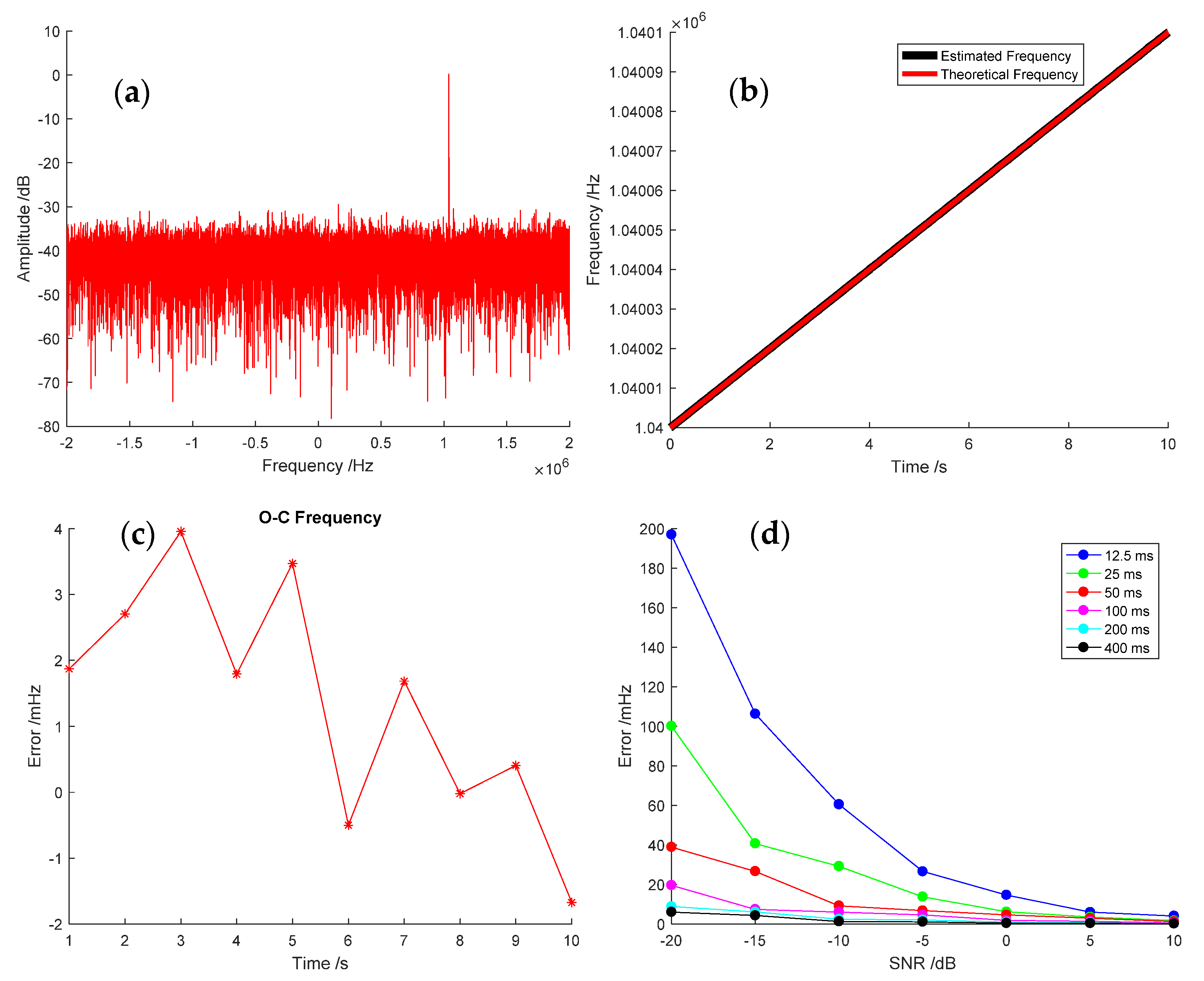
3. Simulation
4. Results
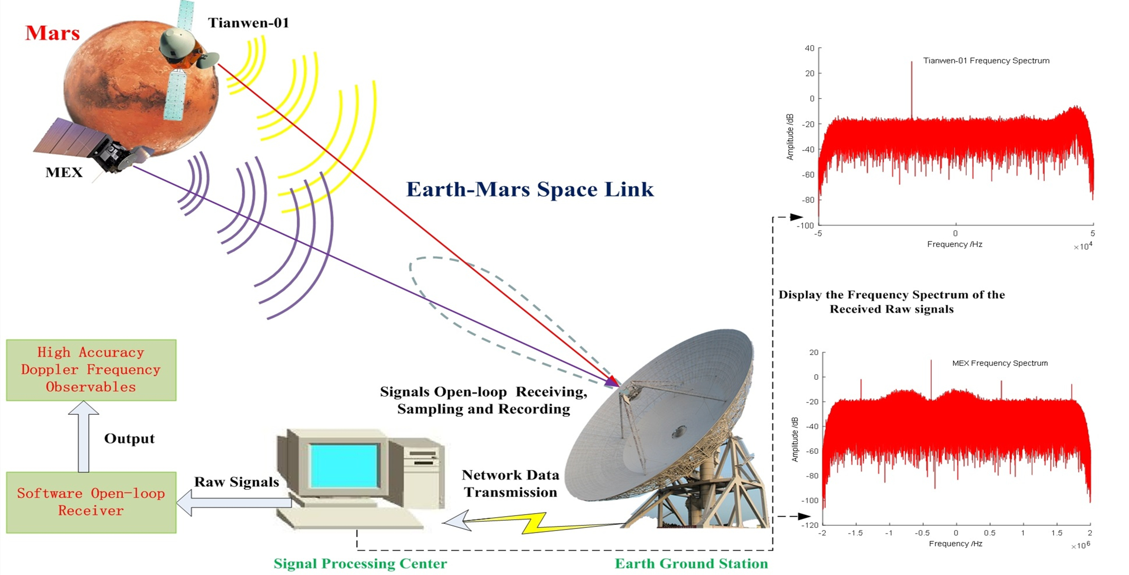
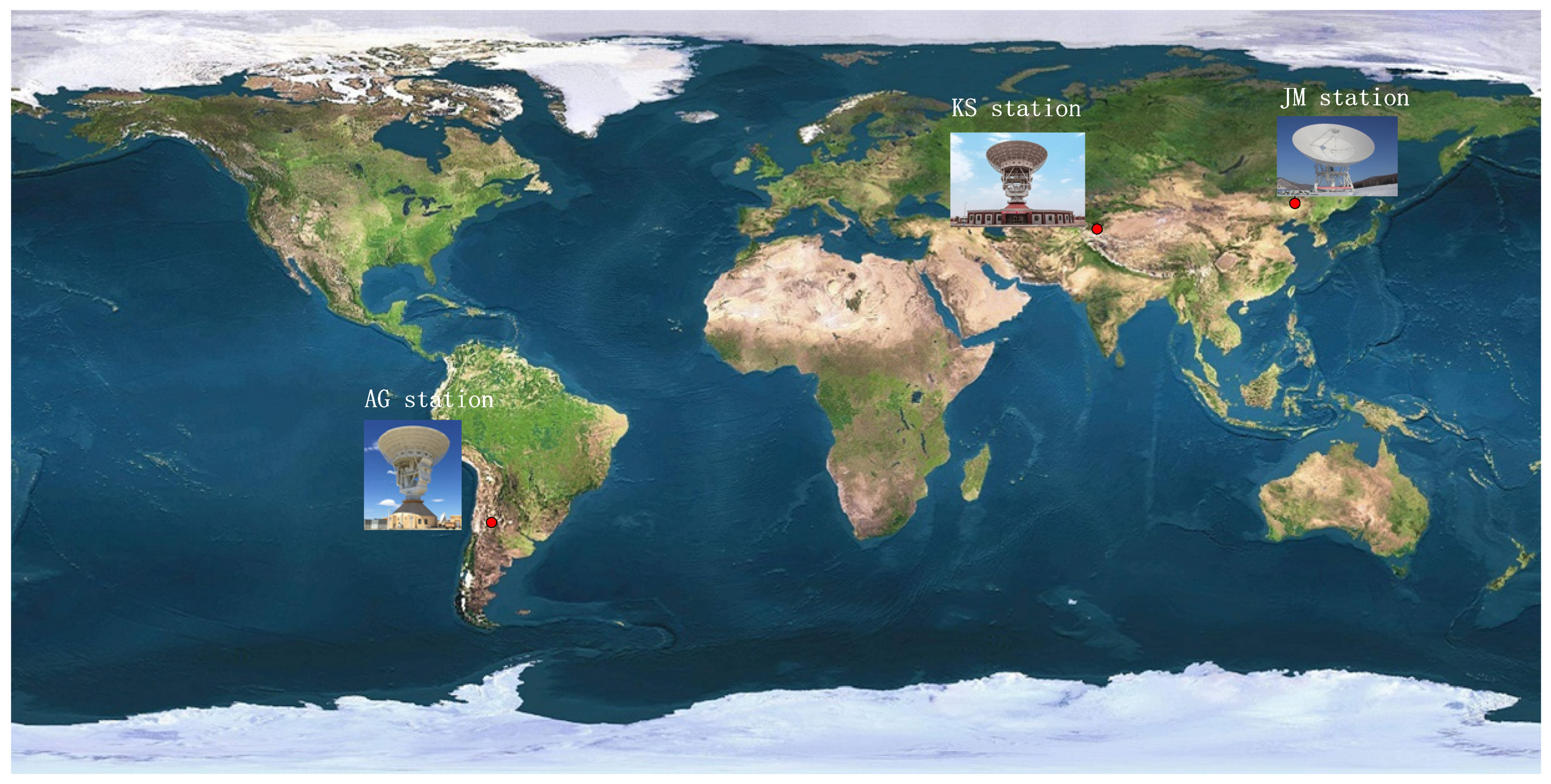
4.1. Mars Express Experiment
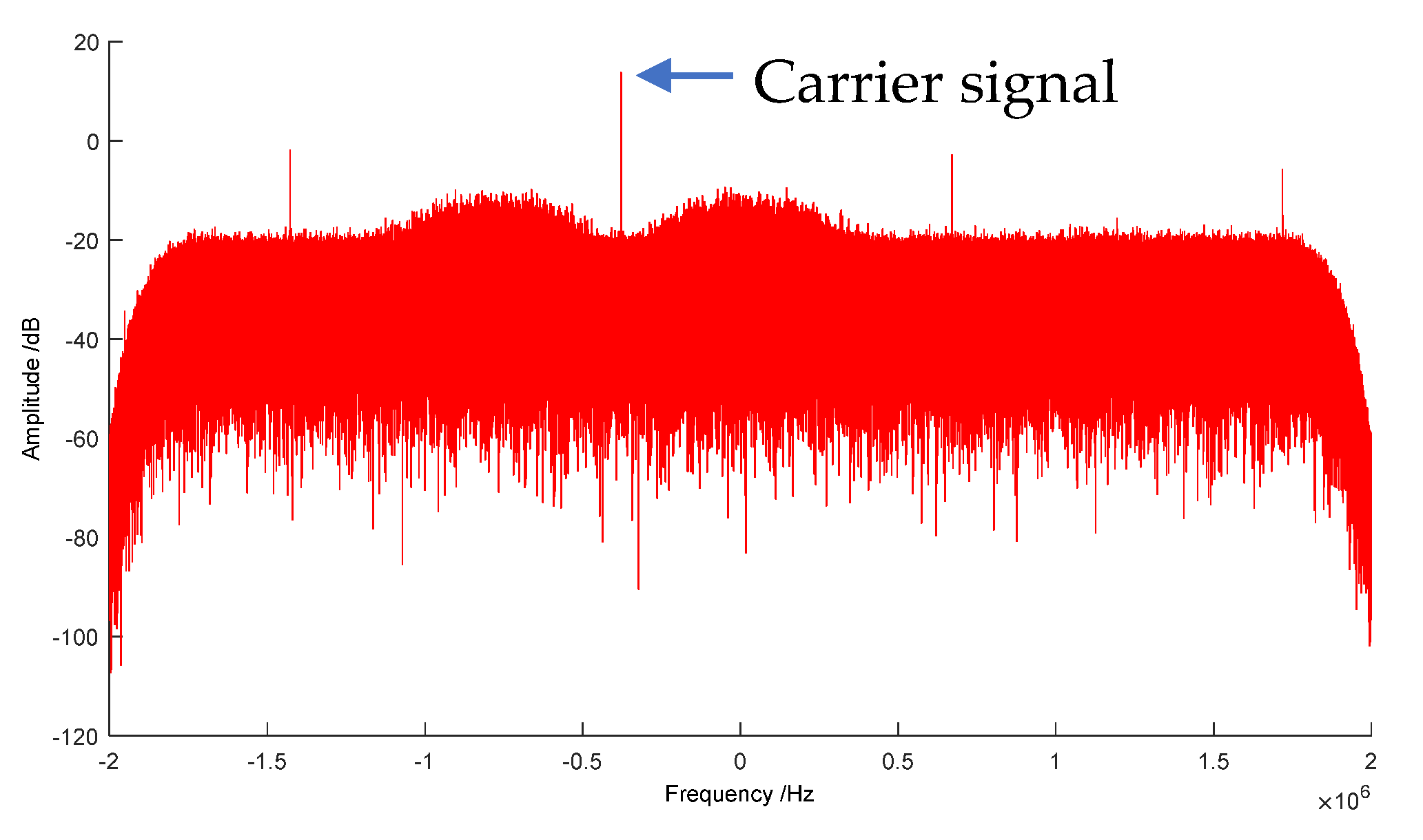
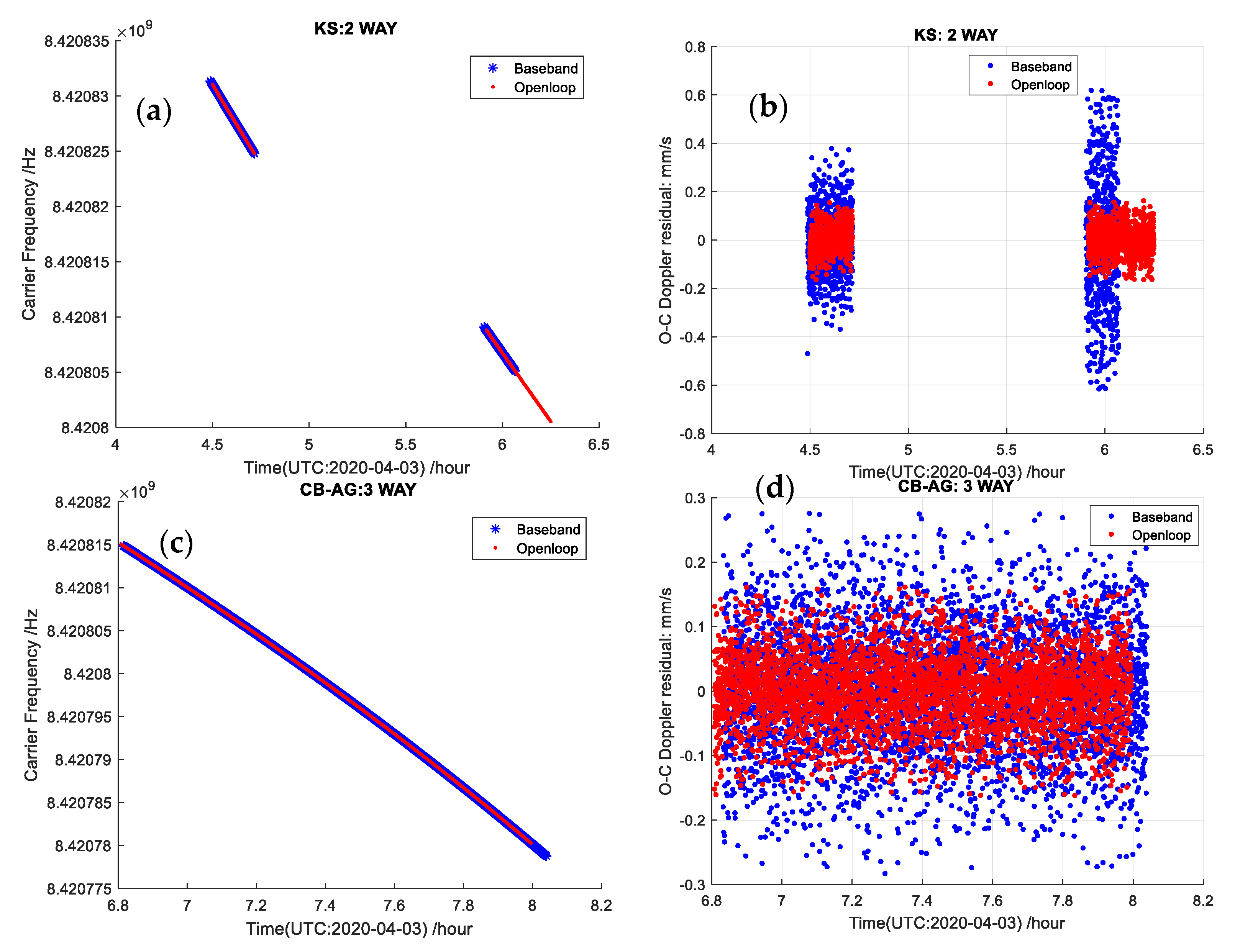
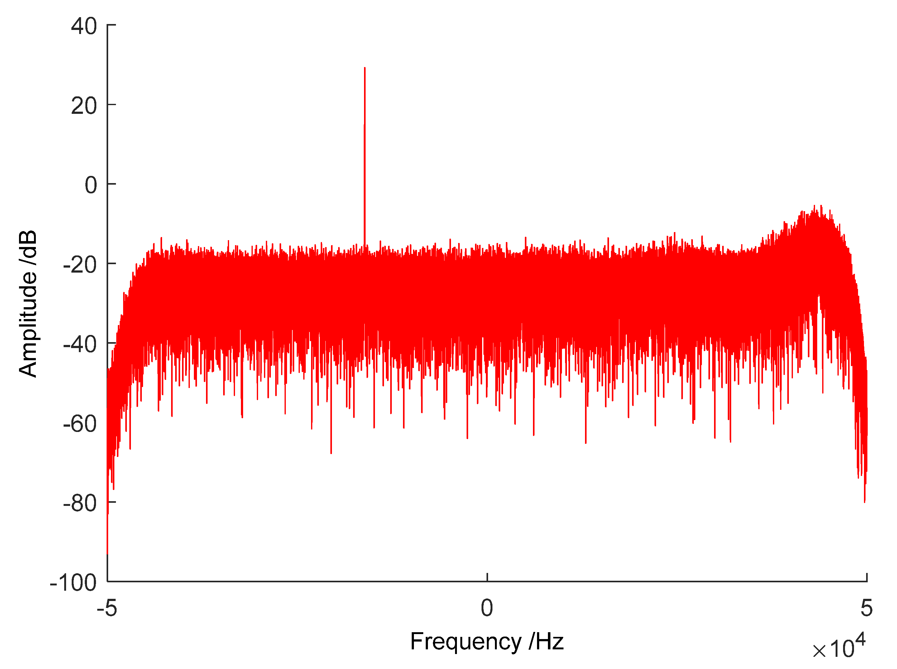
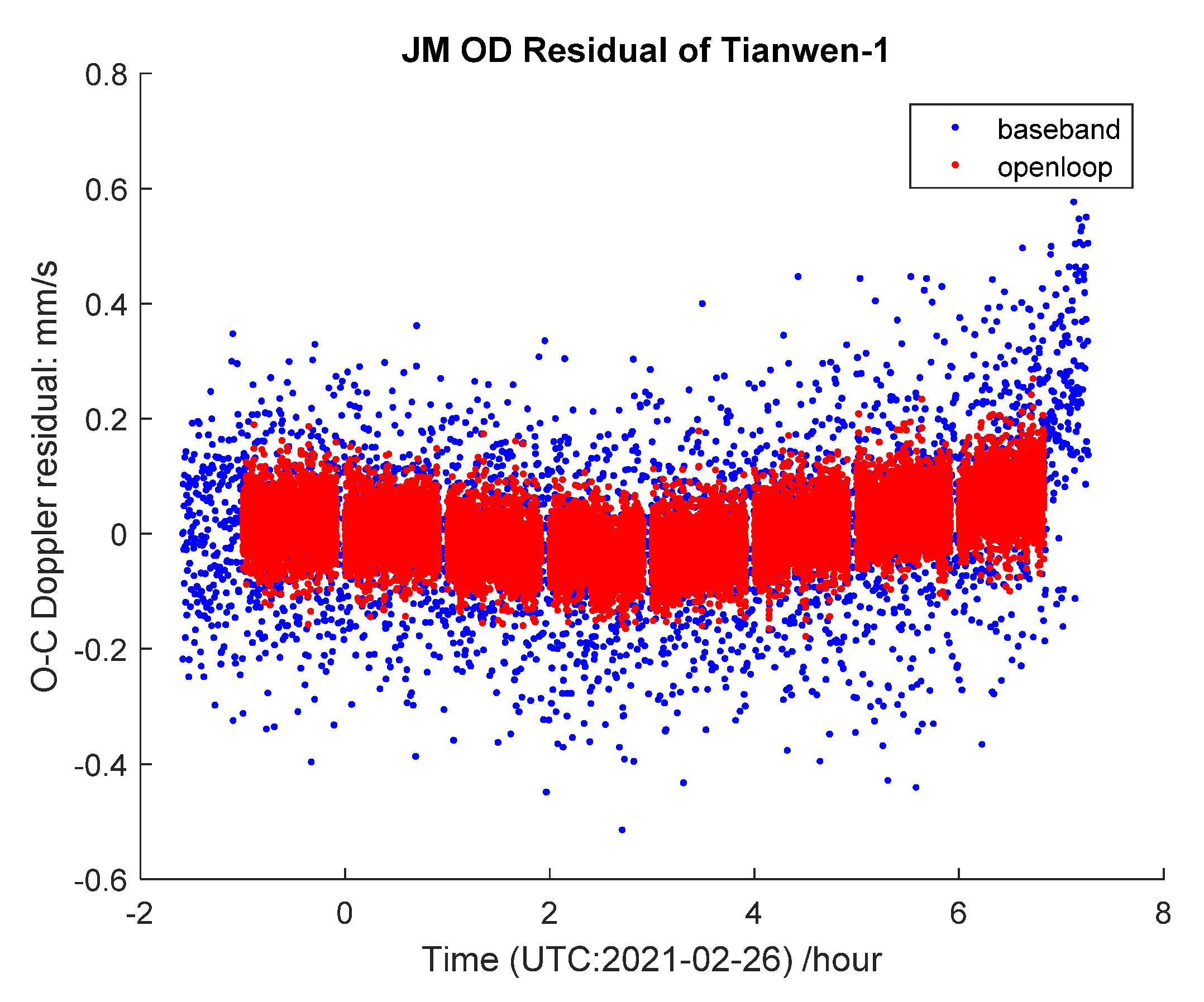
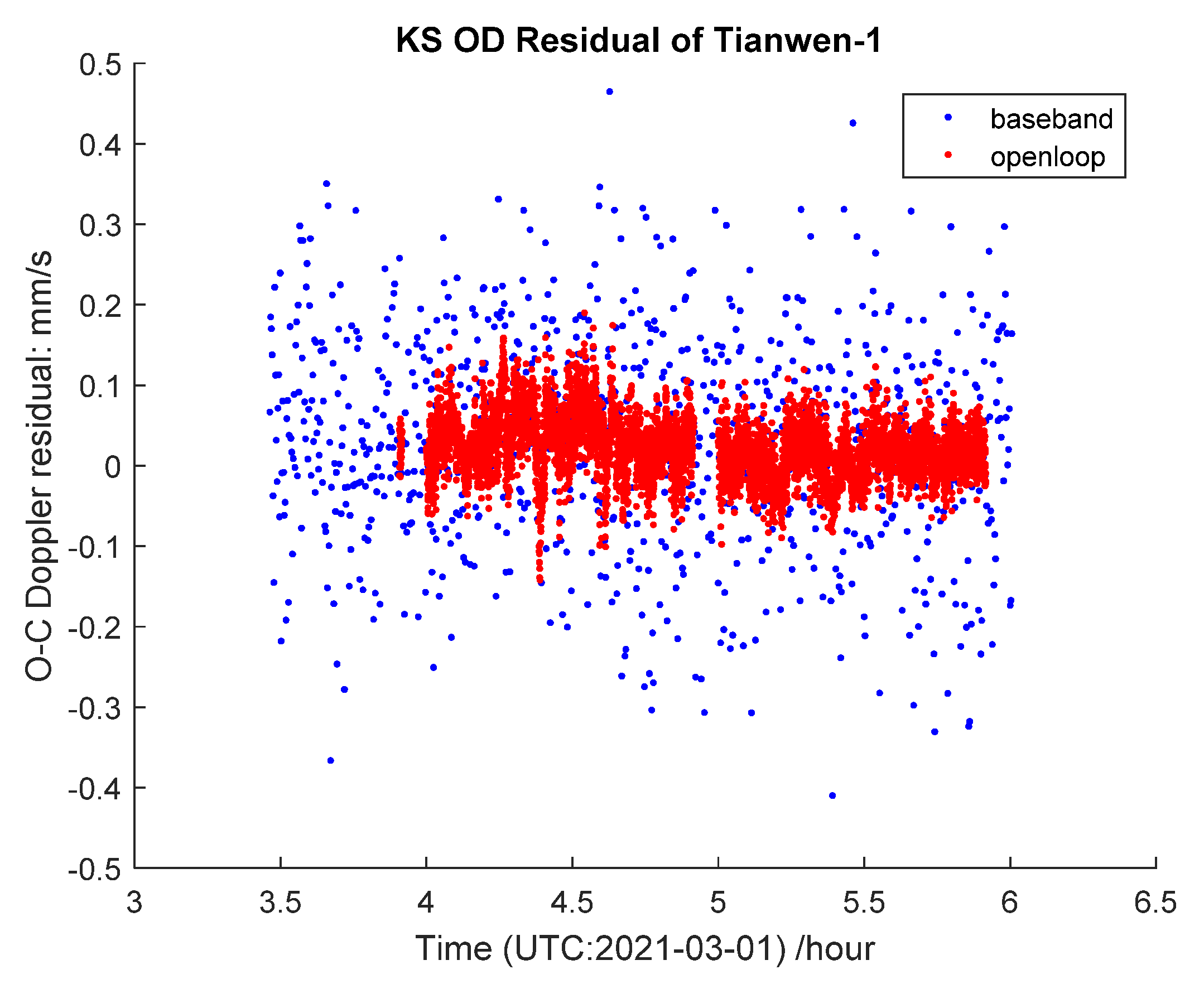
4.2. Signal Processing Results of Tianwen-1
5. Conclusions
Author Contributions
Funding
Institutional Review Board Statement
Informed Consent Statement
Data Availability Statement
Acknowledgments
Conflicts of Interest
References
- Thornton, C.L.; Border, J.S. Range and Doppler Tracking Observables. In Radiometric Tracking Techniques for Deep-Space Navigation; Yue, J.H., Ed.; The Deep-Space Communications and Navigation Systems Center of Excellence, Jet Propulsion Laboratory, California Institute of Technology: Pasadena, CA, USA, 2000; pp. 9–46. [Google Scholar]
- Chang, C.; Pham, T. DSN Telecommunications Link Design Handbook; DSN No. 810-005; Rev, F., Ed.; Jet Propulsion Laboratory: Pasadena, CA, USA. Available online: http://deepspace.jpl.nasa.gov/dsndocs/810-005/ (accessed on 7 June 2021).
- Iess, L.; Di Benedetto, M.; Marabucci, M.; Racioppa, P. Improved Doppler Tracking Systems for Deep Space Navigation. In Proceedings of the 23rd International Symposium on Space Flight Dynamics, Pasadena, CA, USA, 29 October–2 November 2012. [Google Scholar]
- Rosenblatt, P.; Lainey, V.; le Maistre, S.; Marty, J.C.; Dehant, V.; Patzold, M.; van Hoolst, T.; Hauslere, B. Accurate Mars Express orbits to improve the determination of the mass and ephemeris of the Martian moons. Planet. Space Sci. 2008, 56, 1043–1053. [Google Scholar] [CrossRef]
- Duan, J.; Wang, Z. Orbit determination of CE-40s relay satellite in Earth-Moon L2 libration point orbit. Adv. Space Res. 2019, 64, 2345–2355. [Google Scholar] [CrossRef]
- Paik, M.; Asmar, S.W. Detecting high dynamics signals from open-loop radio science investigations. Proc. IEEE 2011, 99, 881–888. [Google Scholar] [CrossRef]
- He, Q.; Yang, Y.; Li, F.; Yan, J.; Chen, Y. Using cross correlation to estimate Doppler frequency. Adv. Space Res. 2020, 65, 1772–1780. [Google Scholar] [CrossRef]
- Chen, W.; Huang, L. Research on Open-Loop Measurement Technique for Spacecraft. In Proceedings of the 27th Conference of Spacecraft TT&C Technology in China, Lecture Notes in Electrical Engineering 323, Guangzhou, China, 9–12 November 2005; Tsinghua University Press: Guangzhou, China, 2015; pp. 185–197. [Google Scholar]
- Bocanegra-Bahamón, T.M.; Calvés, G.M.; Gurvits, L.I.; Cimò, G.; Dirkx, D.; Duev, D.A.; Pogrebenko, S.V.; Rosenblatt, P.; Limaye, S.; Cui, L.; et al. Venus Express radio occultation observed by PRIDE. Astron. Astrophys. 2019, 624, A59. [Google Scholar] [CrossRef] [Green Version]
- Bocanegra-Bahamón, T.M.; Calvés, G.M.; Gurvits, L.I.; Duev, D.A.; Pogrebenko, S.V.; Cimò, G.; Dirkx, D.; Rosenblatt, P. Planetary Radio Interferometry and Doppler Experiment (PRIDE) technique: A test case of the Mars Express Phobos Flyby II. Doppler tracking: Formulation of observed and computed values, and noise budget. Astron. Astrophys. 2018, 609, A59. [Google Scholar] [CrossRef] [Green Version]
- Buccino, D.R.; Kahan, D.S.; Yang, O.; Oudrhiri, K. Extraction of Doppler Observables from Open-Loop Recordings for the Juno Radio Science Investigation. In Proceedings of the 2018 United States National Committee of URSI National Radio Science Meeting, Boulder, CO, USA, 4–7 January 2018; Available online: https://0-ieeexplore-ieee-org.brum.beds.ac.uk/document/8299690 (accessed on 7 June 2021).
- Jian, N.; Shang, K.; Zhang, S.; Wang, M.; Shi, X.; Ping, J.; Yan, J.; Tang, G.; Liu, J.; Qiu, S.; et al. A digital open-loop Doppler processing prototype for deep-space navigation. Sci. China Ser. G 2009, 52, 1–9. [Google Scholar] [CrossRef]
- Shang, K.; Ping, J.; Dai, C.; Jian, N. Open loop doppler tracking in Chinese forthcoming Mars mission. In Proceedings of the International Astronomical Union, IAU Symposium; Volume 261, pp. 209–211. Available online: https://ui.adsabs.harvard.edu/abs/2010IAUS..261..209S/abstract (accessed on 7 June 2021).
- Bedrossian, A. 209 Open-Loop Radio Science. DSN No. 810-005, 209, Rev. D.; Issue Date: 14 February 2019. JPL D-19379; URS CL#19-0898. Available online: https://deepspace.jpl.nasa.gov/dsndocs/810-005/209/209D.pdf (accessed on 7 June 2021).
- Bhaskaran, S. The Application of Noncoherent Doppler Data Types for Deep Space Navigation; TDA Progress Report 42-121; TDA: Putrajaya, Malaysia, 15 May 1995; pp. 54–66. Available online: https://ipnpr.jpl.nasa.gov/progress_report/42-121/121B.pdf (accessed on 7 June 2021).
- Duev, D.A.; Calvés, G.M.; Pogrebenko, S.V.; Gurvits, L.I.; Cimó, G.; Bahamon, T.B. Spacecraft VLBI and Doppler tracking: Algorithms and implementation. Astron. Astrophys. 2012, 541, A43. [Google Scholar] [CrossRef] [Green Version]
- Duev, D.A.; Pogrebenko, S.V.; Cimò, G.; Calvés, G.M.; Bahamón, T.M.B.; Gurvits, L.I.; Kettenis, M.M.; Kania, J.; Tudose, V.; Rosenblatt, P.; et al. Planetary Radio Interferometry and Doppler Experiment (PRIDE) technique: A test case of the Mars Express Phobos fly-by. Astron. Astrophys. 2016, 593, A34. [Google Scholar] [CrossRef] [Green Version]
- Bocanegra-Bahamón, T.M.; Gurvits, L.I.; Calvés, G.M.; Cimò, G.; Duev, D.A.; Pogrebenko, S. VLBI and Doppler tracking of spacecraft for planetary atmospheric studies. In Proceedings of the 14th European VLBI Network Symposium & Users Meeting, Granada, Spain, 8–11 October 2018; Science Press: Granada, Spain, 2018; pp. 1–5. [Google Scholar]
- Zhang, T.; Meng, Q.; Ping, J.; Chen, C.; Jian, N.; Liu, W.; Yao, S.; Yu, Q.; Wang, M.; Li, W.; et al. A real-time, high-accuracy, hardware-based integrated parameter estimator for deep space navigation and planetary radio science experiments. Meas. Sci. Technol. 2019, 30, 015007. [Google Scholar] [CrossRef]
- Tang, J.; Xia, L.; Mahapatra, R. An open-loop system design for deep space signal processing applications. Acta Astronaut. 2018, 147, 259–272. [Google Scholar] [CrossRef]
- Rabiner, L.R.; Schafer, R.W.; Rader, C.M. The chirp z-transform algorithm and its application. Bell Syst. Tech. J. 1969, 48, 1249–1292. [Google Scholar] [CrossRef]
- Han, S.; Zhang, Z.; Sun, J.; Cao, J.; Chen, L.; Lu, W.; Li, W. Lunar Radiometric Measurement Based on Observing China Chang’E-3 Lander with VLBI—First Insight. Adv. Astron. 2019, 10, 7018620. [Google Scholar] [CrossRef]
- Chen, L.; Ping, J.-S.; Liu, X.; Wang, N.; Cao, J.-F.; Chen, G.-M.; Wang, M.-Y.; Li, W.-X.; Zhang, J.-H.; Chen, Y.-Q.; et al. Preliminarily study of Saturn’s upper atmosphere density by observing Cassini plunging via China’s deep space station. Res. Astron. Astrophys. 2020, 20, 102. [Google Scholar] [CrossRef]
- Hao, W.; Lu, M.; Li, Z.; Wang, H.; Fan, M.; Zhu, Z.; Shi, S.; Cheng, C.; Han, S.; Li, H. The high dynamics tracking capability for power descending in Chinese Chang’E-3 mission. Adv. Space Res. 2017, 60, 82–89. [Google Scholar] [CrossRef]
- Chicarro, A.; Martin, P.; Trautner, R. The Mars Express Mission: An Overview. In Mars Express: The Scientific Payload; Wilson, A., Chicarro, A., Eds.; ESA SP-1240; ESA Publications Division: Noordwijk, The Netherlands, 2004; pp. 3–13. ISBN 92-9092-556-6. [Google Scholar]
- The Consultative Committee for Space Data Systems. Delta-DOR Raw Data Exchange Format; Recommended Standard; CCSDS 506.1-B-1; Blue Book: Bloomington, MN, USA, 2013; Available online: https://public.ccsds.org/Pubs/506x1b1.pdf (accessed on 7 June 2021).
- O’Dea, A. 202 Doppler Tracking; DSN No. 810-005, 202, Rev. C.; Issue Date: 22 January 2019. JPL D-19379; CL#19-0432. Available online: https://deepspace.jpl.nasa.gov/dsndocs/810-005/202/202C.pdf (accessed on 7 June 2021).
- Cao, J.; Huang, Y.; Hu, X.; Ma, M.; Zheng, W. Mars Express tracking and orbit determination trials with Chinese VLBI network. Chin. Sci. Bull. 2010, 55, 3654–3660. [Google Scholar] [CrossRef]
- Genova, A. ORACLE: A mission concept to study Mars’ climate, surface and interior. Acta Astronaut. 2020, 166, 317–329. [Google Scholar] [CrossRef]
- Pätzold, M.; Häusler, B.; Tyler, G.L.; Andert, T.; Asmar, S.W.; Bird, M.K.; Dehant, V.; Hinson, D.P.; Rosenblatt, P.; Simpson, R.A.; et al. Mars Express 10 years at Mars: Observations by the Mars Express Radio Science Experiment (MaRS). Planet. Space Sci. 2016, 127, 44–90. [Google Scholar] [CrossRef]
- Le Maistre, S.; Rosenblatt, P.; Dehant, V.; Marty, J.-C.; Yseboodt, M.; Le Maistre, S.; Rosenblatt, P.; Dehant, V.; Marty, J.-C.; Yseboodt, M. Mars rotation determination from a moving rover using Doppler tracking data: What could be done? Planet. Space Sci. 2018, 159, 17–27. [Google Scholar] [CrossRef]
- Dehant, V.; Le Maistre, S.; Baland, R.-M.; Bergeot, N.; Karatekin, O.; Peters, M.-J.; Rivoldini, A.; Lozano, L.R.; Temel, O.; Van Hoolst, T.; et al. The radioscience LaRa instrument onboard ExoMars 2020 to investigate the rotation and interior of mars. Planet. Space Sci. 2020, 180, 104776. [Google Scholar] [CrossRef]
- Kahan, D.S.; Folkner, W.M.; Buccino, D.R.; Dehant, V.; le Maistre, S.; Rivoldini, A.; van Hoolst, T.; Yseboodt, M.; Marty, J.C. Mars precession rate determined from radiometric tracking of the InSight Lander. Planet. Space Sci. 2021, 199, 105208. [Google Scholar] [CrossRef]
- Zou, Y.; Zhu, Y.; Bai, Y.; Wang, L.; Jia, Y.; Shen, W.; Fan, Y.; Liu, Y.; Wang, C.; Zhang, A.; et al. Scientific objectives and payloads of Tianwen-1, China’s first Mars exploration mission. Adv. Space Res. 2021, 67, 812–823. [Google Scholar] [CrossRef]


| Date | Station | Measurement Way | RMS (mm/s) | Remark |
|---|---|---|---|---|
| 3 April | KS | two-way | 0.055 | Open-loop |
| 3 April | KS | two-way | 0.21 | Baseband |
| 3 April | AG | three-way | 0.054 | Open-loop |
| 3 April | AG | three-way | 0.095 | Baseband |
| 16 April | JM | two-way | 0.06 | Open-loop |
| 16 April | KS | three-way | 0.61 | Open-loop |
| 16 April | KS | two-way | 0.053 | Open-loop |
| 16 April | KS | two-way | 0.24 | Baseband |
| Station | Measurement Way | Integration (1 s) | Integration (5 s) | Integration (10 s) | Integration (60 s) | Remark |
|---|---|---|---|---|---|---|
| KS | two-way | 2.99 | 1.70 | 1.18 | 0.45 | 3 April |
| three-way | 3.66 | 1.94 | 1.52 | 0.73 | 16 April | |
| AG | three-way | 3.18 | 1.51 | 1.20 | 1.03 | / |
| JM | two-way | 3.38 | 2.13 | 1.63 | 0.72 | / |
| CDSS | / | 3.3 | 1.82 | 1.38 | 0.73 | Average |
| EVN/VLBA | three-way | / | / | 1.7 | / | Ref. [17] |
| EVN/VLBA | three-way | / | / | 2.0 | / | Ref. [10] |
| NASA/ ESA | two-way | / | / | 1.0 | / | Ref. [10] |
| NASA/ ESA | two-way | 3.2 | / | / | 1.2 | Ref. [4] |
| CVN | three-way | / | 4.14 | / | / | Ref. [28] |
| CVN | three-way | 7.0 | / | / | / | Ref. [19] |
Publisher’s Note: MDPI stays neutral with regard to jurisdictional claims in published maps and institutional affiliations. |
© 2021 by the authors. Licensee MDPI, Basel, Switzerland. This article is an open access article distributed under the terms and conditions of the Creative Commons Attribution (CC BY) license (https://creativecommons.org/licenses/by/4.0/).
Share and Cite
Chen, L.; Ping, J.; Cao, J.; Liu, X.; Wang, N.; Wang, Z.; Zhu, P.; Wang, M.; Man, H.; Fan, F.; et al. Retrieving Doppler Frequency via Local Correlation Method of Segmented Modeling. Remote Sens. 2021, 13, 2846. https://0-doi-org.brum.beds.ac.uk/10.3390/rs13142846
Chen L, Ping J, Cao J, Liu X, Wang N, Wang Z, Zhu P, Wang M, Man H, Fan F, et al. Retrieving Doppler Frequency via Local Correlation Method of Segmented Modeling. Remote Sensing. 2021; 13(14):2846. https://0-doi-org.brum.beds.ac.uk/10.3390/rs13142846
Chicago/Turabian StyleChen, Lue, Jinsong Ping, Jianfeng Cao, Xiang Liu, Na Wang, Zhen Wang, Ping Zhu, Mei Wang, Haijun Man, Fei Fan, and et al. 2021. "Retrieving Doppler Frequency via Local Correlation Method of Segmented Modeling" Remote Sensing 13, no. 14: 2846. https://0-doi-org.brum.beds.ac.uk/10.3390/rs13142846