
Hyperanalytic Wavelet-Based Robust Edge Detection


Communications Department, Politehnica University, 300223 Timisoara, Romania
*
Author to whom correspondence should be addressed.
Remote Sens. 2021, 13(15), 2888; https://0-doi-org.brum.beds.ac.uk/10.3390/rs13152888
Submission received: 21 June 2021
/
Revised: 17 July 2021
/
Accepted: 20 July 2021
/
Published: 23 July 2021
(This article belongs to the Special Issue The Future of Remote Sensing: Harnessing the Data Revolution)
Abstract
:The imperfections of image acquisition systems produce noise. The majority of edge detectors, including gradient-based edge detectors, are sensitive to noise. To reduce this sensitivity, the first step of some edge detectors’ algorithms, such as the Canny’s edge detector, is the filtering of acquired images with a Gaussian filter. We show experimentally that this filtering is not sufficient in case of strong Additive White Gaussian or multiplicative speckle noise, because the remaining grains of noise produce false edges. The aim of this paper is to improve edge detection robustness against Gaussian and speckle noise by preceding the Canny’s edge detector with a new type of denoising system. We propose a two-stage denoising system acting in the Hyperanalytic Wavelet Transform Domain. The results obtained in applying the proposed edge detection method outperform state-of-the-art edge detection results from the literature.
1. Introduction
One of the key operations in remote sensing image processing is edge detection. The result of edge detection is a binary image representing a sketch of that image which carries important information concerning the localization of different targets into the remote sensing image. We can use edge detection mostly for general image processing goals such as segmentation, detection of boundary or recognition of objects.
Edges are high frequency components of an image, localized where sharp transitions of the image intensity appear.
Edge detectors transform a grayscale or color image into a binary image known as an edge map, which preserves almost all the information content carried by the original image. The edge map represents a sparse form of the original image with a reduced number of bits, favorable for further fast processing tasks.
We can classify the edge detection methods in accordance with the basic principles they use.
Gradient-based edge detectors are linear operators exploiting the fact that the value of the image function f(x,y) varies significantly around edge points. We can appreciate this change by computing the gradient of image, ∇f, a vector into two dimensions composed by the partial derivatives of the image with respect to the geometrical coordinates x and y. Pixels with high gradient magnitude are located on edges. The edge direction in a given pixel is perpendicular to the direction of the gradient. Gradient operators in the horizontal and vertical directions, denoted by Gx and Gy, can be computed using convolution masks hx and hy,
The most used edge detection operators are Prewitt, Sobel, Robinson, and Kirsch [1]. Then the edge strength ES(x,y) can be estimated as the gradient vector’s magnitude and so we can detect the edges as the set of pixels having maximum gradients. Taking into account that the systems necessary for the computation of derivatives are high-pass filters, the gradient-based edge detectors are sensitive to noise.
Canny [2] has chosen for the design of gradient operator an analytic approach, defining the following three optimization criteria for the edge detector:
- (a)
- To have a low error rate,
- (b)
- The edge points should be well localized,
- (c)
- To circumvent the possibility to have multiple responses for a single edge.
A simplified description of the algorithmic steps of the Canny’s edge detector follows:
- (1)
- To reduce the sensitivity of the edge detector to noise, a Gaussian filter is applied first;
- (2)
- To compute the gradient magnitude and direction, the derivative operators are used;
- (3)
- To get edges with a one-pixel width, non-maximum suppression is used;
- (4)
- To eliminate weak edges, the threshold with hysteresis is applied.
Another class of edge detectors is composed of zero-crossing edge detectors [3]. In this class, the edges are detected where the second derivative of the image crosses zero. The principal drawback of this second class of edge detectors is the sensitivity to noise, taking into account the fact that the derivation operation represents high-pass filtering. This problem can be solved by convolving the input image with a Gaussian filter impulse response and next applying the Laplacian filter. The sequence of those operations can be changed, due to the linearity of derivation and convolution operations, obtaining the so-called Laplacian of Gaussian (LoG) operator. The response of LoG is not usually thresholded; it is usually inspected whether its sign has changed within the mask of 2 × 2 pixels around the examined point.
A third class of edge detectors is composed of morphological edge detectors. They can be considered as non-linear gradient operators, because they produce, similar to linear gradient operators, edge strength. However, we apply non-linear morphological operations such as: erosion; dilation; or both; to obtain this edge strength [4]. These morphological operators are noise sensitive, additionally.
The image often contains both large and small objects, which can be examined at different scales.
Marr and Hildreth remarked in [3] on the possibility of detecting separately at different scales the contours of objects with different surfaces. The second derivative of a Gaussian is an appropriate filter for the edge detection at a given scale. Thus, they detected the edges at a given scale by finding the localization of zero values of for image f, where Ga(x,y) is a two-dimensional Gaussian distribution and ∇2 is the Laplacian. Other multiscale approaches to edge detection use morphological detectors. One method [5] applies the same morphological edge detector at various scales. A different multiscale edge detection method is based on the combination of the Canny’s detector with the scale multiplication. A truly comprehensive multiscale edge detector is the Wavelets Transform [6]. Mallat has proved the equivalence of a multiscale Canny’s edge detector with the finding of the local maxima of a wavelet transform using a Gaussian smoothing function.
This multiscale edge detection approach combines local maxima of a wavelet transform found at various scales to build the global edge map, or multiplies the wavelet coefficients at two adjacent scales.
1.1. Motivation
The imperfections in the acquisition systems produce images contaminated by noise, requiring robust edge detectors. We can already find different robust edge detectors in the literature. The aim of this paper is to explore a new robust edge detector based on hyperanalytic wavelets [7]. To ensure the robustness to noise, we denoise the image first using hyperanalytic wavelets and next we apply the edge detection. Wavelets-based denoising is an image preprocessing method extensively studied, obtaining impressive results and has numerous applications in image processing. Wavelets have many properties very useful for image denoising:
- (A)
- The wavelet transforms (WT) are sparse representations of images and can be implemented with fast algorithms [6];
- (B)
- There is an inter-scale dependency between the wavelet detail coefficients from two consecutive scales [8]. In the following, the parent coefficients will be indexed by 1 and the child coefficients will be indexed by 2;
- (C)
- The probability density functions (pdf) of wavelet detail coefficients or parent-children pairs of wavelet detail coefficients are invariant to input image transformations [9];
- (D)
- The WT decorrelates the noise component of the input image [6];
- (E)
- (F)
- The CoWT have good directional selectivity and low redundancy.
1.2. Contribution
The first step of our robust edge detection method consists in the application of a hyperanalytic wavelet-based two-stage denoising system. The concept of two stages denoising system was introduced in [12]. The first stage separates the noise component of the acquired image with the aid of a first wavelet-based denoising system, which uses a first HWT (W1 in Figure 1). The noise component extracted by the first stage serves as pilot for the second stage, which is another wavelet-based denoising system. A second HWT (W2 in Figure 1) is used in the second stage. By applying the two-dimensional DWT (2DDWT) to the pilot, we estimate separately, based on (2), the standard deviation σn of each W2 detail sub-band,
where y represents the wavelet detail coefficients of the 2DDWT of the pilot and represents the diagonal detail sub-band of this 2D DWT at the first decomposition level [13].
Then, the Maximum a Posteriori (MAP) filter applied in the W2 domain uses this feature to estimate the standard deviation of the input image’s noiseless component σ using,
where σy represents the standard deviation of the acquired image’s WT pixels. The main advantage of this two stages denoising approach is that it avoids the limitations generally imposed on MAP filters’ denoising scheme as the low Signal-to-Noise Ratio (SNR) or the whiteness of the noise.
We propose to use a marginal Adaptive Soft Thresholding Filter (ASTF), denoted as Sh in Figure 1, in HWT domain as the first stage and an improved bishrink filter [8] in the HWT domain as the second stage. The bishrink improvements result from the utilization of directional windows, better parent sub-images, extending the method and a more accurate computation of local standard deviations.
The second step of the proposed robust edge detection method involves the use of the Canny’s edge detector.
We compare the results of the proposed method with results obtained applying directly the Canny’s edge detector to the acquired image.
1.3. Related Work
In case of Gaussian noise, the robust edge detection is performed in [14] by fusing gradient-based edge detection using a small-scaled isotropic Gaussian kernel and anisotropic directional derivatives of a large-scaled anisotropic Gaussian kernel. The authors of [14] embedded the fused edge map into the algorithm of the Canny’s detector, obtaining a robust edge detector with two additional modifications: equalization of contrast and a noise-dependent lower threshold.
In other papers, mixed noise obtained as a combination of Gaussian and impulse noise is considered. The authors of [15] proposed a robust edge detector based on an algorithm in three steps:
- 1.
- Detecting the step and linear edges from images corrupted by mixed noise (exponential and impulse) without smoothing. The authors of [15] substituted the Gaussian smoothing filter with a statistical classification technique;
- 2.
- Detecting thin-line edges, as a series of outliers using the Dixon’s r-test;
- 3.
- Suppressing the spurious edge elements and connecting the isolated missing edge elements.
The authors of [16] proposed another approach in cases of mixed noise. Their algorithm is based on testing whether a window of size r × r is divided into two sub-regions, with significant differences in the local value of the gray level between the neighborhoods of pixels adjacent to a given pixel, using an edge-height model to extract edges of sufficient height from images corrupted by both Gaussian and impulse noises.
The speckle noise (which is multiplicative in nature) affects the images generated by coherent RADAR systems. The authors of [17] proposed a robust edge detector for the processing of this type of images. For robust edge detection in images affected by multiplicative noise with Weibull distribution, the paper [17] defines and compares several new techniques. The authors accomplish edge detection by comparing ratios of locally adjacent irradiance averages such as local irradiance averages, optimal single order statistics and best linear unbiased estimates using order statistics to an appropriate threshold.
Another challenging category of images is the class of biomedical images that are affected by different types of noise: readout noise, thermal noise and photon noise. The authors of [18] proposed a new robust edge detector for biomedical images; they perform the edge detection using an adaptive algorithm based on local signal energy variation computed into a 3 × 3 window.
The authors of [19] proposed an edge detection method robust to impulse noise, based on denoising. In this study, they conceived a new combination of mean and median filters named the Switching Adaptive Median Filter With Mean Filter (SAMFWMF), which has an additional shrinkage window. It represents a new smoothing filter conceived to optimally remove or minimize the presence of impulse noise, even at high intensity levels. This denoising method preserves edge details with good accuracy.
2. Materials and Methods
The wavelet representation is optimally sparse for signals produced by piecewise smooth functions that are composed of low-order polynomials segments separated by jump discontinuities, requiring, by an order of magnitude, fewer coefficients than the Fourier basis to approximate within the same margin of error. The sparsity of the wavelet coefficients of many real-world signals enables near-optimal signal processing based on simple thresholding (keeping the large coefficients and removing the small ones), the base of many state-of-the-art deterministic and statistical image processing methods as: compression (JPEG2000) or denoising. We can decompose any signal u into a dictionary D (whose columns are l elementary atoms) in the form:
where ak represents synthesis coefficients. Among the most popular dictionaries, we can find WTs and Discrete Cosine Transform (DCT). We will denote in the following a wavelet dictionary D = W and the corresponding synthesis coefficients a = w. Hence, we will write the decomposition of the signal u into a wavelet basis as:
U = Ww.
We will regard the denoising problem as a regularization problem. The noise affects randomly the intensity values of each pixel in a noisy image. Hence, by regularizing the pixel intensity values, we can remove the noise.
Researchers from many fields have intensively studied the methods of regularization, gathering a large volume of papers published on this topic.
One of these methods is the Least Absolute Shrinkage and Selection Operator (LASSO) regularization and in case of additive noise it has the form:
where y represents the coefficients of the WT of the acquired image and λ is a constant called regularization parameter.
For , we can express the right-hand part of Equation (6) as:
Taking into account the definition of the lp norm,
we can remark that the two exponentials in the right-hand side member of Equation (7) represent the pdf of Gaussian and Laplacian distributions:
The Gaussian distribution characterizes the additive noise, and the Laplacian distribution characterizes the noiseless component of the WT of the input image. Therefore, we can further process Equation (7) as:
which represents the general equation of a MAP filter. Considering the fact that the two pdfs in (9) represent the priors for the ASTF MAP filter [7], we remark that this filter solves the LASSO regularization problem cases of denoising images affected by Gaussian additive noise.
2.1. Hyperanalytic Wavelet Transform
The DWT is a non-redundant WT, implementable with the aid of the fast Mallat’s algorithm. It has some drawbacks [8]:
- Since wavelets are bandpass functions, the wavelet coefficients tend to oscillate around singularities;
- The wavelet coefficients oscillation pattern around singularities is significantly perturbed even by small shift of the signal;
- The wide spacing of the wavelet coefficient samples (the calculation of the wavelet coefficients involves interleaved sampling operations in discrete time and high-pass filtering), resulting in a substantial aliasing. The inverse DWT transformation (IDWT) cancels this aliasing, of course, if the wavelet coefficients are not changed. Any wavelet coefficient processing operation, as seen in thresholding; filtering; or quantization, leading to artifacts in the reconstructed signal.
We can correct the last two drawbacks of the DWT by increasing its redundancy.
The complex DWT (CDWT) proposed in [7] is a CoWT whose Mother Wavelet (MW) is quasi-analytic, corrects the drawbacks of the DWT and has a two-times redundancy. We can compute it with the aid of two DWT trees. These trees are connected in parallel, one computing the real part of the CDWT, with the aid of a MW ψ, and the other computing the imaginary part of the CDWT, with the aid of the Hilbert transform (denoted by H, in the following) of the MW used for the computation of the DWT on the first tree, H{ψ}. This is equivalent to a single tree CoWT whose MW is equal to the analytic signal associated to the MW ψ, ψa ψ H{ψ}. Further, it is equivalent to the computation of the DWT of the analytic signal associated with the input signal with the aid of the real MW ψ. Hence, the operation of analytic signal generation commutes with the computation of DWT associated with the real MW. We will name this property, using an expression taken from electronics, reduction at the input. The CDWT is a quasi-shift invariant as well [7].
We can achieve the extension of WT to 2D by separable filtering along rows and then columns. If we want to apply the DWT to two-dimensional signals, we need to use the DWT extension to two dimensions, namely the 2D DWT. At the foundation of the 2D DWT implementation are the concepts of separable multiresolution and two-dimensional wavelet basis. Similar to the classical DWT, the 2D DWT is a non-redundant transform which has the 1D DWT drawbacks already mentioned as well as poor directional selectivity. Indeed, it has only three preferential orientations: horizontal, vertical and diagonal.
The authors of [20] reported a second order statistical analysis of the 2D DWT coefficients, which highlights their inter-scale and intra-band dependency. They have modeled the input images as wide sense stationary bivariate random processes and derived closed form expressions for the wavelet coefficients correlation functions in all possible scenarios: inter-scale and inter-band, inter-scale and intra-band, intra-scale and inter-band as well as intra-scale and intra-band.
The generalization of the analyticity concept in 2D is not obvious, because there is not unique definition of the Hilbert transform in this case [21]. The analytical signal associated with a real signal is a complex function whose real part is equal to the real signal and whose imaginary part is equal to the Hilbert transformation of the real signal. Therefore, the analytic signal associates real numbers to complex numbers (pairs of real numbers, whose set has a structure of algebra). A hyperanalytic image is the analytical signal associated to a real image (function of two variables) and is a function with four components: the real part, the imaginary part versus the first variable of the input image, the imaginary part versus the second variable and the imaginary part versus both variables of the input image. Hence, a hyperanalytic image is a two-times complex function, which associates real numbers to sets of four ordered real numbers, named hypercomplex numbers. The set of hypercomplex numbers has the structure of algebra. The multiplication table associated with this algebra defines every relation between the imaginary units of the hypercomplex numbers and implies the specific properties of the algebra. For each different multiplication table, we obtain a different definition of the hypercomplex image. For example, see the following multiplication table:
which corresponds to quaternions algebra [22]. This is a non-commutative, associative hypercomplex algebra; used to construct a hypercomplex WT. Due to the missing commutativity of the quaternions hyperanalytic algebra, this hyperanalytic WT is irreducible at the input. In [7], the authors have chosen the commutative hypercomplex algebra with the following multiplication table, proposed in [23]:
Starting from the real MW ψ(x,y) and scaling function (SF) φ(x,y), the authors of [7] defined the following hypercomplex MW and SF:
where Hx denotes the Hilbert transform computed on rows and Hy the Hilbert transform computed on columns.
The corresponding hyperanalytic WT is abbreviated HWT. Its detail coefficients represent the scalar product of the input image f(x,y) and the hypercomplex wavelets (generated by translations and dilations of the MW ) and its approximation coefficients represent the scalar product of the input image and the functions (generated by translations and dilations of the hypercomplex SF ):
We can reduce the HWT at the input because [7]:
where represents the hyperanalytic form of the input image. Therefore, the HWT is reducible at the input and computed as 2D DWT of the hyperanalytic form of the input image. In consequence, the HWT implementation has a redundancy of four because it uses four branches, each one implementing a non-redundant 2D DWT. The first branch processes the input image. The second and third branches process 1D Hilbert transforms applied to the input image. The 1D Hilbert transform from the second branch is computed across the lines of the input image (Hx) and the 1D Hilbert transform from the third branch is computed across the columns of the input image (Hy). Finally, the fourth branch processes the result obtained after the computation of the two 1D Hilbert transforms of the input image (Hy(Hx)). The scheme for the HWT implementation proposed in [7] contains two blocks. The first one computes the hypercomplex input image and the four 2D DWTs, whose output sequences are: d1, d2, d3 and d4. The second block improves the directional selectivity of HWT. Through the linear combinations of detail coefficients belonging to each sub-band of each of the four 2D-DWTs, described in Equation (16), we can obtain the HWT directional selectivity’s enhancement:
The 2D-DWT has poor directional selectivity, it does not detect the difference between the directions of the two principal diagonals, because it has only three preferential orientations: 0, π/4 and π/2. Because of (16), the HWT has better directional selectivity than 2D-DWT, having six preferential orientations: ±atan (1/2), ±π/4 and ±atan (2).
The complete second order statistical analysis of HWT reported in [24] shows the stronger dependency of the magnitude of HWT coefficients in intra-scale scenarios than those of 2D DWT. Therefore, the parent–child dependency of hyperanalytic wavelet coefficients is important and global MAP filters, as the bishrink filter is, are preferable for the denoising in HWT domain.
In [9] is shown that zero-mean Laplace pdf models the univariate distribution of the wavelet coefficients of any deterministic image considered independently and that the following pdf can be used to model parent–child pairs of wavelet coefficients,
where the parent coefficients are indexed by 1 and the child coefficients are indexed by 2. Therefore, the pdfs of wavelet detail coefficients or parent–child pairs of wavelet coefficients are invariant to the selection of the input image, when it is not affected by noise.
2.2. Global MAP Filters Applied in Wavelet Domain
Taking into account the equivalence between the MAP filters and regularization problems [25,26], we can remark that one of the most efficient parametric denoising methods implies the use of MAP filters. The problem solved by a MAP filter is to evaluate w from a single noisy measurement, y = w + n, where n is noise. The MAP filters apply a Bayesian approach to estimate the a posteriori (or ‘posterior’) distribution: the probability distribution of w, given the measurement y, i.e., , contains all the information that we can infer about a given y. In cases where the posterior distribution of w is unimodal (having a unique maximum in W) then the value W represents the MAP estimate of w. We can compute the posterior distribution with the aid of Bayes’ theorem,
Generally, it is easy to calculate , named the likelihood of w given the data . The inference w = W implies that the noise can be expressed as n = y − W. Hence, the likelihood is , where pn is the noise’s pdf. The MAP estimation of w is given by (10). The solution of (10) is a marginal MAP filter [27], if w and n are scalars. When w and n are vectors, the solution of (10) is a global MAP filter [8].
The principal advantage of denoising methods which operate in a transform domain with sparse representation (as seen for example in the WT) is the shorter computation time required because the volume of data are reduced by the transform.
We can successfully apply denoising methods in the wavelet domain [28].
This class includes different methods: non-parametric techniques (as the hard or soft thresholding filtering [13]); semi-parametric techniques [29]; or MAP filters-based techniques [8,27,30,31,32]. Based on the observation x = s + ni, such a denoising method supposes the following steps:
- 1.
- Computation of the WT of the observation: and separation of approximation and detail coefficients;
- 2.
- Non-linear filtering of detail coefficients and restructuration of WT by the concatenation of approximation coefficients with the new detail coefficients;
- 3.
- Computation of the inverse WT (IWT).
In the following, we will denote the WT of the observation by y = WT{x}, the WT of the noiseless component of the input image by w = WT{s} and the WT of the noise by n = WT{ni}.
Hence, the denoising methods based on the association of wavelets and MAP filters are algorithms that apply a MAP filter in a WT domain: the 2D DWT [13], the SWT [27], the DTCWT [11] or the HWT [7]. We will give, in the following, three examples of MAP filters which can be associated with WTs.
The zero order Wiener filter minimizes the mean square approximation error (MSE). It can be seen as a marginal MAP filter where both priors: Wpn and Wpw are Gaussians,
This solves the Tikhonov regularization problem in case of AWGN.
The soft thresholding filter [13], is a shrinkage filter, asymptotically optimal in a minimax MSE sense over a large variety of smoothness spaces. The marginal ASTF is a marginal MAP filter with a Gaussian prior stpn and a Laplacian prior stpw:
The following input–output relations for the corresponding systems are obtained solving (10) with the priors in (19), (20) or (21):
in case of the Wiener filter,
where:
and the value of the threshold t is given by:
for the marginal ASTF and:
for the bishrink filter.
Bishrink Filter
The bishrink filter is a member of shrinkage filters class that processes the wavelet detail coefficients as shown in (26). As any shrinkage filter, the bishrink filter has a dead zone represented in the plane of the magnitudes of parent and child wavelet detail coefficients, (y1, y2) as a circle with the center in the origin of the plane and with the ray:
Relation (27) represents a threshold for the magnitude of the vector . As a consequence of the bivariate distribution of parent and child wavelet detail coefficients already mentioned, it results that the wavelet detail coefficients belonging to the dead zone have small magnitudes. Hence, the majority of the pixels of the image from the filter input will have zero intensity at their output. The dead zone of the bishrink filter is responsible for a part of distortions introduced by this filter.
In practice, are realized the following operations to compute the values of the threshold t. First is computed the 2D DWT of the input image and the diagonal detail sub-band at the first decomposition level () is retained, to estimate the noise standard deviation , using (2). When the bishrink filter is associated with 2D DWT for denoising, is scalar. When the bishrink is associated with CoWT, the estimation of the noise standard deviation is a vector, containing noise standard deviation estimations for each branch of the CoWT.
The next step is to compute the WT of the input image and to separate the sub-images corresponding to each sub-band and decomposition level, to create the sets of child wavelet coefficients y2. The corresponding coefficients at the next decomposition level represent the parent wavelet coefficients y1. The sub-images of parent wavelet coefficients are extended by doubling the lines and columns to obtain the same size as the sub-images of child wavelet coefficients, in order to compute in each pixel the magnitude of vector y: , required by (26) [8]. The next step supposes the computation of the local noiseless component’s standard deviations in each sub-band, obtaining a sub-band adaptive bishrink filter, or locally in each sub-band, using moving windows of size 7 × 7, obtaining a local adaptive bishrink filter. For each position of the window, a local estimation of the noisy child wavelet coefficients variances, is realized, and next is applied relation (3) using the noise standard deviation already estimated to obtain the local estimation of noiseless components variances:
The next step supposes the computation of the bishrink thresholds as:
and the filtering can be done by applying (26),
Starting from (30), we can compute the sensitivity of the bishrink filter with the threshold obtaining the following expression:
which is a decreasing function of the threshold. Therefore, any increasing of the threshold magnitude caused by features erroneous estimations, produces an increase of the absolute value of the sensitivity, , thus degrading the performance of the bishrink filter. The value of the threshold increases if the estimation of noise standard deviation increases, or , decreases, even if the features are perfectly estimated. Hence, the performance of the bishrink filter deteriorates with the noise power increase. The performance of the bishrink filter is lower in homogeneous regions, where is small and higher on the edges, where is large.
2.3. Multiplicative Noise
The model of the acquired image in case of multiplicative noise is:
x = sni.
This model is used in cases of Synthetic Aperture Radar (SAR) images [31,32,33] or SONAR images [34,35]. The statistical model of the speckle noise is presented in Appendix A. By homomorphic treatment, the model of multiplicative noise can be reduced to the model of additive noise. Taking in both sides of the previous equation the natural logarithm, it is obtained:
which represents an additive noise model. From a historical point of view, it first appeared in some statistical despeckling filters acting in the spatial domain, as the Lee [36], Kuan [37], Frost [38] and Gamma [39] filters. The Gamma despeckling system is a MAP filter built by considering that the noiseless component of the acquired image’s logarithm has a logΓ distribution. Next, Walessa and Datcu [40] proposed another statistical despecklization system in spatial domain, entitled the Model-Based Despeckling (MBD) filter. This algorithm uses a Gauss Markov Random Field (GMRF) model for textures and preserves the edges between uniform areas with the aid of an adaptive neighborhood system. The authors of [40] used an Expectation Maximization (EM) algorithm to estimate the texture parameters with the highest evidence. Using a stochastic region-growing algorithm, they detected borders between homogeneous areas, locally determining the neighborhood system of the Gauss Markov prior. The authors of [40] found strong scatterers in the ratio image (also named method noise image), obtained by dividing the acquired image to the filtered result image, and replaced them. This way, textures, edges and strong scatterers can be preserved and well reconstructed. Additionally, it is possible to use the estimated model parameters for further image interpretation methods. In [41], a spatial domain MAP despeckling filter is proposed. It transforms the speckle in additive noise by homomorphic treatment and uses a heavy-tailed Rayleigh distribution as a model for the noiseless component of the logarithmically transformed SAR image. The authors of [41] derived their model, based on the alpha-stable family of distributions. They estimate the model parameters of the noiseless component with the aid of Mellin transform.
log(x) = log(s) + log(ni),
The Non Local Means (NLM) algorithm [42] was readily extended by the authors of [43] to the case of SAR images despeckling. A similar approach, entitled the Probabilistic Patch-Based (PPB) algorithm, is proposed in [44]. The authors of [44] developed a new similarity measure, well suited to SAR images, and obtained excellent results on test images. As usual, the denoising methods applied in a transformed domain have better despecklization results. The authors of [45] used 2D DWT to apply the MBD algorithm in the wavelet domain, obtaining a new despecklization algorithm, which improves the performance of MBD and reduces dramatically the execution time. The authors of [46] proposed another statistical despecklization algorithm based on 2D DWT, named the Spatially Adaptive Wavelet Homomorphic Shrinkage algorithm; it uses the Cauchy distribution for the useful wavelet coefficients model and the Gaussian distribution for the wavelet coefficients of the noise, and minimizes a mean absolute error (MMAE) criterion. The complete name of this algorithm is SA-WBMMAE. The authors of [27] used SWT and conceived a marginal MAP filter based on Pearson statistical model. The Gamma filter was applied in [47] in the SWT domain, obtaining the so-called Homomorphic Gamma-Wavelet MAP (H.Γ-WMAP) filter, which has better performance and shorter execution time than the Gamma filter. Another despecklization method applies a MAP filter, based on Generalized Gaussian (GG) prior to the SWT domain [48]. The big advantage of SWT is that it shifts invariance, however, the directional selectivity of SWT is poor. The authors of [49] further developed the idea in [48], to improve the despeckling performance, proposing the texture energy of the wavelet coefficients as a feature of their classification. The name of this algorithm is MAP-S. The 2D DWT and the SWT use real wavelets, while some despeckling algorithms are conceived using complex wavelets [50,51]. The authors of reference [50] present the generation of Daubechies complex MWs, also named Symmetric Daubechies (SD) MWs. These MWs have all the properties of the real Daubechies MWs and an additional symmetry property; they use 2D-DWTs computed using these MWs in a despecklization algorithm associated with an elliptical soft thresholding filter [13]. They named this despecklization algorithm the Complex Wavelet Coefficient Shrinkage (CWCS) filter. The BM3D algorithm [52], conceived for additive noise, was adapted in [53] to the case of SAR images in two variants. The first variant, named HBM3D, uses a homomorphic approach and embeds the BM3D algorithm. The second variant, named SAR-BM3D, consists of the modification of some steps of the BM3D algorithm, as for example the substitution of the DWT by the SWT and the substitution of the collaborative Wiener filter by an LLMMSE adaptive filter. We have found in the literature some studies dedicated to the comparison of different despecklization methods for SAR images [47,50,53,54]. The authors of [47] compared more than 30 different spatial domain speckle filters. One of the conclusions of this study is that the MBD filter of Walessa and Datcu represents one of the best solutions concerning the preservation of details and smoothing in homogeneous regions. The authors of [50] present a comparison between the CWCS filter and other despecklization systems such as, Lee, Kuan, Frost, Geometric, Kalman and Gamma. The CWCS equals the performance of the standard speckle filters in the case of a low Signal-to-Noise Ratio (SNR) and outperforms this performance in the case of high SNR. The authors of [53] present a more recent comparison of different despecklization methods. They compare eight despeckling systems. These filters are the following: the well-known Frost filter, the SA-WBMMAE algorithm, the PPB algorithm and its homomorphic variant, the H-PPB algorithm, the MAP-S algorithm, the H-BM3D algorithm and the SAR-BM3D algorithm.
Considering that log(s) represents the noiseless component of the input image and that log(ni) represents the additive noise, we can apply the HWT-marginal ASTF or HWT-Bishrink denoising associations, which are additive noise-denoising kernels. Due to the decorrelation effect of WTs, the statistical model of the HWT of log(ni) is Gaussian in case of the HWT-marginal ASTF association and bivariate Gaussian in case of the HWT-Bishrink association. These priors were considered for log(ni) in the majority of references about wavelet-based despeckling already cited, as seen for example in [45] or [46]. Based on experiments, in different papers, as for example [9], was proved that the statistical model of the wavelet detail coefficients of noiseless images is characterized by a heavy tail distribution, such as a Laplacian, and that this model is invariant to different transformations, such as the logarithm. Therefore, the statistical model of HWT of log(s) is Laplacian in case of HWT-marginal ASTF association and bivariate symmetric Laplacian in the case of HWT-Bishrink association.
The estimation of the noiseless component of the image perturbed by multiplicative noise supposes the inversion of the result’s logarithm. As shown in [47], the homomorphic treatment introduces a small bias. It can be rejected by using a mean correction block. The proposed denoising system uses two mean computation blocks. The first computes the mean of the acquired image, which, taking into account the fact that the expectation of speckle noise is unitary, is equal to the mean of its noise-free component. The second mean computation block is used to correct the expectation of the result. It computes the statistical mean of the image at the output of the block that inverts the logarithm. We subtract this mean from the denoising result and we add the mean of the acquired image computed by the first mean computation block. Taking into account the considerations about the sensitivity of the bishrink filter from the end of the previous section, a block for sensitivity reduction could be included in the denoising system [34,35].
2.4. Proposed Denoising Method
We apply the denoising strategy having the architecture in Figure 1 as an additive noise-denoising kernel. In Figure 1, we utilize for the first denoising system the association of the marginal ASTF (Sh) with HWT (W1). To compute this HWT, we have used the Daubechies MW with two Vanishing Moments (VM). Supposing the Additive White Gaussian Noise (AWGN) model for the input image, we obtain the image after the computation of W1:
The diagonal detail sub-bands of the four 2D-DWTs, used to compute the HWT W1, at the first decomposition level (), are retained, to estimate the four noise standard deviations, , using (2). Next is realized the estimation of local noiseless components standard deviations in each sub-band and at any decomposition level, using moving windows 7 × 7 pixels in size. For each window position, the local variances of noisy child wavelet coefficients are estimated and after is applied the relation (3) using the noise standard deviations already estimated, to obtain the local estimation of noiseless components standard deviations . The following step is to apply the marginal ASTF, whose input–output relation is:
where t1 is the threshold computed with the following relation:
The result of the estimation realized by the first stage, s1, is obtained after the computation of the four inverse 2D DWTs. By computing the difference of images x and s1:
we can obtain the pilot.
The second denoising system in Figure 1 associates the HWT (W2) with an improved variant of bishrink filter.
First, a second HWT (denoted as W2 in Figure 1) is applied to the pilot , in order to compute the standard deviations of the wavelet detail, , of each W2 detail sub-band. Next, W2 is applied to the image x. Both HWTs denoted as W2, are computed using the Daubechies 9/7 biorthogonal MW. The HWT of x is used for the bishrink filtering. Next, we separate the child y1 and parent y2 wavelet coefficients for any sub-band and pair of successive decomposition levels. We extend the parent sub-images by resizing with factor 2, obtaining sub-images of same size as the corresponding child sub-images. Next, we estimate the local standard deviation of the noiseless component of the input image, , for each sub-band and decomposition level with the aid of constant array elliptic estimation windows. The principal axes of those ellipses are oriented following the preferential orientations of the sub-bands: ±atan (1/2), ±π/4 and ±atan (2). The authors of [55] introduced the elliptic directional windows in conjunction with the 2D DWT. The authors of [7] generalized this idea. Another source of bias for the noiseless component estimation is the small size of the estimation window [56]. Despite the fact that the mean of detail coefficients equals zero for the ensemble of the entire image, the mean of the detail coefficients in the estimation window could be different of zero. Therefore, we compute first the mean in the estimation window and next we compute the local variances. Extracting the square roots of variances, we obtain the sub-images containing the estimation of local standard deviations of the image y, in each sub-band and decomposition level.
The estimations of the local standard deviations of the child coefficients of the noiseless component of the input image, , can be done now based on the estimations using (3). We can improve the estimation of the local standard deviations of the noiseless component of the input image in (3), taking into account the dependency between the parent and child wavelet detail coefficients of noiseless images: the standard deviation of parent coefficients is two times bigger than the standard deviation of the child coefficients [20]. The estimation of the local standard deviations of the parent coefficients of the noiseless component of the input image can be done similarly with the estimation for the child coefficients . Hence, we have estimated the local standard deviations of the noiseless component of the input image as:
Next, we compute the bishrink threshold in every sub-band and decomposition level using:
We apply relation (30) to realize the bishrink filtering:
Inverting the HWT (), the result is obtained.
When we deal with remote sensing images, we precede the additive noise-denoising kernel by a block for the logarithm computation and a block for the acquired image’s expectation estimation. The additive noise-denoising kernel is followed in the case of remote sensing images by a mean correction block and a block for the logarithm inversion.
2.5. Performance Measures
The Peak Signal-to-Noise Ratio (PSNR) is one of the objective quality measures for denoising algorithms:
where the Mean Square Error (MSE), another objective quality measure, can be computed with:
Np represents the number of pixels of the considered image, sq are the pixels of the noiseless component and are the pixels of the denoising result.
A third objective quality indicator of a denoising method is the Structural SIMilarity Index (SSIM). It highlights the similarity of the noiseless component of the acquired image, X, with the denoising result Y, having same size and is calculated as:
where and are expectations of X and Y, and are the variances of X and Y and is the covariance of X and Y. PSNR, MSE and SSIM are quality indicators which necessitate the knowledge of the noiseless component as reference. We can use MSE for the evaluation of the quality of an edge detection algorithm as well if we dispose of a reference edge map.
The following quality indicators do not necessitate the knowledge of the noiseless component. The Equivalent Number of Looks (ENL) gives a quantitative appreciation of the treatment of a homogeneous region selected:
We can obtain input and output ENLs, applying the same procedure in the same region for the acquired and treated images. The ratio of output and input ENLs represents the ENL enhancement. Unfortunately, denoising methods with oversmoothed results, affecting some features of the original scene such as edges, could have good ENL enhancement.
Recently, the authors of [33] proposed in the context of SAR images denoising a quality measure, named despeckling evaluation index (DEI), which takes into account the treatment of edges. We can subjectively evaluate the quality of denoising with the aid of the method noise image. For a good despeckling algorithm, the method noise image does not contain details of the scene.
3. Results
We evaluate the proposed approach on both synthesized and real images. To assess the performance of the proposed method on synthesized images, we have carried simulations using natural images, such as Lena, Boat and Barbara; which have been used previously to evaluate other image processing methods. Lena and Boat images contain dominant structural features such as edges, lines, corners, etc., and most of the texture of those images is far from periodic. Conversely, the Barbara image contains dominant quasi-periodical textural features (mostly corresponding to clothes). All test images have a size of 512 × 512. We have added independent and identically distributed (i.i.d.) white Gaussian noise to the images at different PSNRs determined by the variance of the noise, . We additionally synthesized speckle noise, which follows a Rayleigh distribution with a unitary mean. Computing the square root of a sum of squares of two zero-mean white Gaussian noises, having same variance, we have generated the noise with Rayleigh distribution. Varying the value of this variance, we obtained images corresponding to different number of looks (NL) denoted by L [27].
Wavelet decomposition was carried out up to level L0 = 7. We have implemented all algorithms in MATLAB using the WaveLab Toolbox [57].
We have considered aerial SAR [58], SONAR [35] and SENTINEL-1 [59] images as real remote sensing images. We have selected these types of images to be as different as possible in order to highlight the universality of the proposed edge detection method. The aerial SAR image used in the first example of the application of the proposed edge detection method on real remote sensing images is acquired with a NASA/JPL Airborne SAR—synthetic aperture RADAR system mounted aboard a modified NASA DC-8 aircraft using linear detection. During data collection, the plane flew at 8 km over the average terrain height of the mountains in Switzerland. The number of looks of the acquired image, L, equals 2. A satellite providing multiple looks of the SAR image is the object of the second example of treating real images. It is a Sentinel-1 Stripmap Ground Range Detected High resolution (GRDH) image; in the case of Sentinel-1 Stripmap image, the SAR signal processor uses the complete data history and the full synthetic aperture to produce the highest possible resolution, which correspond to a Single Look Complex (SLC) SAR image. The amplitude image corresponding to a SLC SAR image is obtained by quadratic detection. The intensity image corresponding to a SLC SAR image is obtained as the square of the amplitude image. Multiple looks may be generated by averaging intensity SLC SAR images over azimuth and/or range resolution cells. Ground Range Detected (GRD) products consist of focused SAR data that has been detected, multi-looked and projected using an Earth ellipsoid model to ground range. The Sentinel-1 Stripmap GRDH image used in the second example of applying the proposed edge detection method to real remote sensing images has a number of looks L = 8. It represents a segment of the border between the Agulhas current and the coast of South Africa. For the third example of the application of the proposed edge detection method to remote sensing images, we have selected a SONAR image. This sea-bed SONAR image shows the Swansea wreck stranded in Le Goulet Bay near Brest during World War I. It was acquired by a military SONAR system possessed by GESMA and has a number of looks L = 1.
3.1. Images Affected by Synthesized Noise
In the case of AWGN noise, we have obtained the following results. For all three images: Lena, Boats and Barbara, the results obtained using the proposed edge detection method are compared with results obtained applying directly the Canny’s edge detector to the noisy image. We have computed the edges’ MSE, taking as reference the edge map of the original noiseless image obtained using Canny’s edge detector. The results for the image Lena are shown in Table 1. We show in Figure 2 some results corresponding to the last line in Table 1.
On the first line of Figure 2, the input (noise-free) image and the edge map obtained applying Canny’s edge detection method to the input image are presented. On the second line of Figure 2, we see the noisy image and the edge map obtained applying directly Canny’s edge detection method. We show the denoised image and its edge map on the third line of Figure 2. In Figure 3, we compare the results obtained applying the proposed method with the results of the robust edge detection method in [14], for σn = 15.
Taking as reference the edge map obtained by applying the Canny’s detector to the noiseless component of the input image, we computed the edges’ MSE for the edge maps in Figure 3. The MSE value obtained for the proposed method equals 0.06. The value obtained for the method in [14] equals 0.11. Hence, the proposed method is more robust against noise than the method in [14].
In Table 2, we analyze the image Boat.
We have counted the missing edge pixels for the proposed method and the false edge pixels introduced by the Canny’s edge detector when applied directly to noisy image. As in the case of Lena image, the edges’ MSE and the number of edge pixels missed by the proposed method are smaller than the edges’ MSE and the number of false edge pixels introduced by the Canny’s detector when applied directly on noisy image, for all the values of noise standard deviation.
We compare in Figure 4 the edge maps obtained applying the Canny’s detector directly to noisy image and proposed method for σn = 30.
The proposed edge detection method is robust against noise even when the noise power is high. In Table 3 we analyze the image Barbara.
We compare in Figure 5 the edge maps obtained when applying the Canny’s detector directly to a noisy image and the proposed method for σn = 30. We can remark the same behavior of the proposed edge detection method concerning the robustness against noise as in the case of images Lena and Boat.
The PSNR and SSIM improvements are objective quantitative measures of performance for a denoising system not related directly with the visual aspect of the result. Generally, we can appreciate the visual aspect by direct inspection. In case of synthesized speckle noise, on the left column in Figure 6, the Lee, Kuan and Frost despeckling filters with a window size of 7 × 7 are visually compared with the MBD algorithm in [40] and with the proposed despeckling method, using the reference image proposed in [40]. On the right column of Figure 6, we see represented the edge maps obtained by applying the Canny’s edges detector to the corresponding images from the left column. As it can be observed by analyzing the right column in Figure 6, all the despeckling methods compared improve the edge detection realized by the Canny’s edge detector (shown in the first image of the right column), but the edge map obtained applying the proposed despeckling method is one of the best.
We compare, in Table 4 and Table 5 some despeckling methods, using the image Lena perturbed by synthesized speckle noise.
There are three different values of the noise variance corresponding to three different Numbers of Looks, L: 1, 4 and 16.
3.2. Real Remote Sensing Images
An aerial SAR image represents the object of our first example of real images treatment. We show on left column of Figure 7 the images, which characterize the proposed denoising system.
The first image on the left column is that acquired by the SAR system. The second image on the left column is the result of the first stage denoising system and the third image represents the result of proposed denoising method. We show in the right column of Figure 7 the edge maps of corresponding images from the left column obtained by applying the Canny’s edge detector. To better appreciate the visual quality of the proposed denoising method, we show in Figure 8, zooms in images corresponding to the same region of the acquired image, first stage result and final denoising result.
To more deeply explore the denoising mechanisms described, we have analyzed the noise rejected by both stages of the proposed denoising system. We resume the conclusions of the noise analysis in the third column of Table 6. We present, in the second column of Table 6, the ENL values corresponding to the blocks of the proposed denoising system. Because all ENL values are higher than 1, we can conclude that these images are not single-look images.
A satellite multiple looks SAR image is the object of the second example of treating real images. We present this Sentinel-1 Stripmap Ground Range Detected High resolution (GRDH) image in left part of Figure 9 [59].
We show, in the right part of Figure 9, the result obtained applying the Canny’s edge detector. Almost all the speckle was removed by the multilooking procedure used to generate the image from the left part of Figure 9. Therefore, the edges map, represented in the right part of the figure, does not contain false edges. Some edge pixels are missing in this edges map as a consequence of the over-smoothing realized by the multilooking procedure, but we can perceive the structure of the scene from this edge map.
A SONAR image is the object of the third example of treating real images. We show on left column of Figure 10 the images describing the proposed denoising system. The first one is the image acquired by the SONAR system.
The second image on the left column is the result of our first stage despeckling system and the third image on the left column represents the result of proposed despeckling method. We show on the right column of Figure 10 the corresponding edge maps of the images from the left column, obtained by applying the Canny’s edge detector. We can remark, analyzing the left column of Figure 10, that the speckle in this example severely affects the original image. This is because this image has a reduced number of looks, L = 1. Observing the image from the second line and left column of Figure 10, we can see that the first stage of the denoising system is not able to completely remove the speckle. Analyzing the image from the third line and left column of Figure 10, we can see that the second stage of the proposed denoising system completely removes the speckle noise. Regarding the image from the first line and right column in Figure 10, we observe that the Canny’s edge detector introduces numerous false edges in case of the original noisy image. The number of false edges remains high even after the application of the first stage of the proposed denoising system (the image on the second line and right column). The proposed edge detection method is robust against speckle noise. We did not observe false edges in the image from the third line and right column in Figure 10, where the SWANSEA wreak can be easily recognized.
4. Discussion
Based on the results presented in the previous section, we will consider in the following the merits and the drawbacks of the proposed edge detection method.
4.1. Images Affected by Synthesized Speckle
Analyzing Table 1, it can be seen that in the case of the image Lena perturbed by AWGN, the proposed method outperforms Canny’s detection method for all values of the noise standard deviation in terms of edges’ MSE values. As a consequence of the analysis in Figure 2, it can be affirmed that in case of the Lena image perturbed by AWGN, the Canny’s edge detector is not robust against noise, despite the utilization of a Gaussian filter in the first step of the algorithm, introducing numerous false edges when it is applied directly to noisy image. The proposed method misses some edges because of the smoothing effect of the denoising method selected. Analyzing Figure 3 by visual inspection, we observe some false edges in case of the method proposed in [14], which cannot be observed in case of the proposed edge detection method. Therefore, the proposed method has a performance superior to the edge detection method proposed in [14]. Similar remarks can be formulated analyzing Table 2 and Figure 4 for the image Boats and Table 3 and Figure 5 for the image Barbara, concerning the superiority of the proposed method versus the direct application of the Canny’s detection method in case of natural images perturbed by AWGN.
We have additionally studied the effect of the proposed edge detection method in the case of synthesized speckle noise. We can observe visually, analyzing Figure 6, that the classical despeckling filters (Lee, Kuan and Frost) are not able to eliminate the entire noise; this effect is more visible in homogeneous regions. Moreover, the classical despeckling filters blur textures and edges, erasing weak contours. Visually, the best results between classical despeckling filters belong to Frost filter. The MBD algorithm has better performance than classical despeckling filters concerning textures and contours, but some noisy pixels remain in the homogeneous regions. The filter proposed here has the best performance, eliminating practically all the noise from the homogeneous regions and preserving textures and edges. The results shown on the last line of Figure 6 prove the anisotropy of the proposed denoising method, which is consequence of the improved directional selectivity of HWT. As it can be observed, analyzing the right column in Figure 6, the edge map obtained applying the proposed despeckling method is the best. We have compared quantitatively the proposed despeckling method with state-of-the-art methods, in the case of synthesized speckle noise in Table 4 and Table 5. The H-BM3D algorithm has the best PSNR results, followed closely by the SAR-BM3D algorithm (Table 5). The results obtained applying the denoising method proposed here are good, outperforming the results obtained with other wavelet-based denoising methods: PPB, MAP-S, SA-WBMMAE, HWT-Bishrink, HWT-marginal ASTF, and the method in [48] (Table 4 and Table 5). Comparing the results obtained by applying the HWT-Bishrink denoising association with the results of the proposed denoising method, we suggest that the idea of two stages and the proposed improvements of the bishrink filter are effective, and further, our algorithm is faster than SAR-BM3D and H-BM3D algorithms.
4.2. Real Remote Sensing Images
We have continued by applying the proposed edge detection method on three real remote sensing images. In case of the aerial image shown in Figure 7, the speckle strongly affects the original image (L = 2). The first stage of the proposed denoising system is not able to remove completely the speckle, whereas the second stage of the proposed denoising system does completely remove the speckle. As in the case of synthesized images, the Canny’s edge detector is not robust against speckle noise. Even after the application of the first stage of the proposed denoising system, the number of false edges remains high, and the proposed edge detection method is robust against noise. We do not observe false edges in the last image in Figure 7. To appreciate visually better the effects of the proposed despeckling method, in Figure 8 are presented zooms in the images in Figure 7. Indeed, the first denoising stage does not reject all speckle noise and the result of proposed denoising system is slightly oversmoothed. To quantitatively appreciate the proposed despeckling system, we have computed the ENLs in Table 6. Our first stage denoising system increases the ENL but is not able to reject entirely the speckle noise. The complete denoising system completely rejects the speckle and increases more the ENL. Hence, the proposed despeckling system has a good performance in the case of aerial SAR images degraded by speckle, despite the small value of the number of looks, but slightly smooths the input image. This over-smoothing prevents the generation of false edges but erases some weak edges.
The multiple looks SAR images, as shown in Figure 9, represents the second example of treating real remote sensing image with the proposed edge detection method, and is obtained by applying a multilooking procedure to Single Look Complex (SLC) SAR images acquired by satellites. The multilooking procedure reduces the speckle, but also reduces the spatial resolution of the SLC SAR image. An alternative to the multilooking procedure which does not reduce the spatial resolution is the despecklization of the SLC SAR image. A very interesting procedure for the despecklization of SLC SAR images is based on the estimation of the rugosity of the scene; this estimation can be performed by evaluating locally the Hurst exponent of the scene. Different semi-local Hurst exponent estimations can be done using the DTCWT [60,61,62]. The corresponding despeckling methods are reported in [63]. The authors of [63] estimated the Hurst parameter by using low resolution coefficients, which are relatively free of noise and the energy of high-resolution level coefficients most affected by noise are corrected according to the estimated parameter. The performance of estimators in [63] is analyzed in [64].
The third example of applying the proposed edge detection procedure to remote sensing images refers to SONAR images, more precisely to the SONAR image in Figure 9. The proposed edge detection method erases some weak edges as consequence of the smoothening effect of the proposed denoising method, but the form of the wreck is easily to perceive based on the last image in Figure 10, despite the reduced number of looks, L=1, of the original image. Conversely, we cannot perceive the form of the wreck analyzing the first two images in the right column in Figure 10. This proves the superiority of the proposed denoising method in comparison with the denoising method based on the association HWT-marginal ASTF.
4.3. Comparison with Modern Despeckling Methods
Deep learning in remote sensing has become a modern direction of research, but it is mostly limited to the evaluation of optical data [65]. The development of more powerful computing devices and the increase of data availability has led to substantial advances in machine learning (ML) methods. The use of ML methods allows remote sensing systems to reach high performance in many complex tasks, e.g., despecklization [66,67,68,69,70,71,72,73,74,75,76,77], object detection, semantic segmentation or image classification. These advancements are due to the capability of Deep Neural Networks to automatically learn suitable features from images in a data-driven approach, without manually setting the parameters of specific algorithms. The Deep Neural Networks act as universal function approximators, using some training data to learn a mapping between an input and the corresponding desired output.
In the following, we present some of the ML methods for despeckling, found in two very recent references, firstly in [65]. Inspired by the success of image denoising using a residual learning network architecture in the computer vision community, [66] in [67] was introduced a residual learning Convolutional Neural Network (CNN) for SAR image despeckling, named SAR-CNN, a 17-layered CNN for learning to subtract speckle components from noisy images in a homomorphic framework. As in the case of the proposed despeckling method in this paper, the homomorphic approach is performed before and after feeding images to a denoising kernel, which in case of [67] is represented by the neural network itself. In this case, multiplicative speckle noise is transformed into an additive form and can be recovered by residual learning, where log-speckle noise is regarded as residual. An input log-noisy image is mapped identically to a fusion layer via a shortcut connection, and then added element-wise with the learned residual image to produce a log-clean image. Afterwards, denoised images can be obtained by the logarithm inversion. The SAR-CNN is trained on simulated single-look SAR images. However, to ensure a better fidelity to the actual statistics of SAR signal and speckle, it is retrained on real SAR data using multi-looked images as approximate clean references.
Wang et al. [68] proposed the ID-CNN, for SAR image despeckling, which can directly learn denoised images via a component-wise division-residual layer with skip connections. Therefore, homomorphic processing is avoided, but at a final stage the noisy image is divided by the learned noise to yield the clean image. This approach makes sense, considering the multiplicative nature of noise. Of course, a pointwise ratio of images may easily produce outliers in the presence of estimated noise values close to zero. However, a tanh nonlinearity layer placed right before the output performs a soft thresholding thus avoiding serious shortcomings.
In [69], Yue et al. proposed a novel deep neural network architecture specifically designed for SAR despeckling. It models both speckle and signal itself as random processes, to better account for the homogeneous/heterogeneous nature of the observed cell. Working in the log-domain, the pdf of the observed signal can be regarded as the result of a convolution between the pdfs of clean signal (unknown) and speckle. The authors of [69] used a CNN to extract image features and reconstruct a discrete RADAR Cross Section (RCS) pdf. It is trained by a hybrid loss function which measures the distance between the actual SAR image intensity pdf and the estimated one that is derived from convolution between the reconstructed RCS pdf and prior speckle pdf.
The unique distribution of SAR intensity images was considered in [70]. A different loss function, which contains three terms between the true and the reconstructed image, is proposed in [70]. These terms are, the common L2 loss; the L2 difference between the gradient of the two images and the Kullback–Leibler divergence between the distributions of the two images. The three terms are designed to emphasize the spatial details, the identification of strong scatterers, and the speckle statistics, respectively.
In [71], the problem of despeckling was tackled by a time series of images. The authors utilized a multi-layer perceptron with several hidden layers to learn non-linear intensity characteristics of training image patches.
Again, using single images instead of time series, the authors of [72] proposed a deep encoder–decoder CNN architecture with a focus on a weakness of CNNs, namely feature preservation. They modified U-Net [73] in order to accommodate speckle statistical features.
Another notable CNN approach was introduced in [74], where the authors used a NLM algorithm, while the weights for pixel-wise similarity measures were assigned using a CNN. The network takes as input a patch extracted from the original domain image, and outputs a set of filter weights, adapted to the local image content. Two types of CNN were conceived to implement this task; the first type is a standard CNN with 12 convolutional layers, while the second type is a 20-layer CNN which includes also two N3 layers to exploit image self-similarities. These layers associate the set of its K nearest neighbors with each input feature, which can be exploited for subsequent nonlocal processing steps. Training for both types of CNN is both on synthetic data and on real multi-looked SAR images. The results of this approach, called CNN-NLM, are impressive, with feature preservation and speckle reduction being clearly observable.
One of the drawbacks of the aforementioned algorithms is the requirement of noise-free and noisy image pairs for training. Often, those training data are simulated using optical images with multiplicative noise. This is of course not ideal for real SAR images. Therefore, one elegant solution is the noise2noise framework [75], where the network only requires two noisy images of the same area. The authors of [75] proved that the network is able to learn a clean representation of the image given the noise distributions of the two noisy images are independent and identical. This idea has been employed in SAR despeckling in [76]. The authors make use of multitemporal SAR images of a same area as the input to the noise2noise network. To mitigate the effect of the temporal change between the input SAR image pairs, the authors multiples a patch similarity term to the original loss function.
Some of the ML methods for SAR images despeckling, already mentioned, are discussed in the second very recent publication, [77], as well. We find very useful Table 2 in [77], which present 31 relevant deep learning-based despeckling methods with their main features. Between these methods, we can find the SAR-CNN, the ID-CNN and the CNN-NLM methods.
Based on [65] and [77], it can be observed that most ML-based despeckling methods employ CNN-based architectures with single images of the scene for training; they either output the clean image in an end-to-end fashion or propose residual-based techniques to learn the underlying noise model.
The despeckling method proposed in this paper is faster and requires less computational resources than the ML-based methods, due to the sparsity of HWT (in conformity with the property (A) mentioned at the end of the Section 1.1), it does not use any training and does not necessitate any learning methodology.
With the availability of large archives of time series thanks to the Sentinel-1 mission, an interesting direction for the ML-based despeckling is to exploit the temporal correlation of speckle characteristics for despeckling applications. Acting in the space domain, these methods require the statistical model of the speckle. On the contrary, the proposed despeckling method acts in the Hyperanalytic Wavelet Transform Domain. Due to the statistical properties (D) and (C) of the wavelet coefficients, mentioned at the end of Section 1.1, the proposed method does not necessitate the knowledge of the speckle’s statistical model. Due to the statistical property (B) of the wavelet coefficients, mentioned at the end of Section 1.1, the proposed despeckling method already exploits the spatial correlation of wavelet detail coefficients. We consider a good idea to exploit the temporal correlation of wavelet detail coefficients, using the available archives of time series.
One critical issue of both ML-based and proposed despeckling methods is the over-smoothing. Many of the CNN-based methods and the proposed despeckling method perform well in terms of speckle removal but are not able to preserve weak edges. This is quite problematic in the despeckling of high-resolution SAR images of urban areas and for robust edge detection in particular.
Another problem in supervised deep learning-based despeckling techniques is the lack of ground truth data. This problem affects the validation of the proposed despeckling method as well, because some objective quality indicators, as for example the PSNR or the SSIM cannot be computed without reference. A solution could be the utilization of optical images of the same scenes, but frequently such images are not accessible or have different parameters as for example size or contrast. In many studies on ML-based despecklization, this problem is more acute, because the training data set is built by corrupting optical images by multiplicative noise. This is far from realistic for despeckling applied to real SAR data. Therefore, despeckling in an unsupervised manner would be highly desirable and worthy of attention.
5. Conclusions
The goal of this paper is to improve Canny’s edge detection robustness against Additive White Gaussian and speckle noise by preceding this detector with a new two-stage Hyperanalytic Wavelet Transform (HWT)-based denoising algorithm.
The HWT transform is flexible, four times redundant, and quasi-invariant to translation, with good directional selectivity, which is useful in many signal and image processing applications. We have performed a simple implementation of this transform, based on the reduction to the input principle, which permits the heritage of the previous results obtained in the framework of two-dimensional separable wavelets theory. Any orthogonal or biorthogonal real Mother Wavelets (MW) can be used for the HWT computation.
In both stages of the proposed denoising algorithm, MAP filters in the HWT domain are used. We have proved the equivalence between the Adaptive Soft Thresholding Filter (ASTF) (whose marginal form is used in the first stage of the proposed denoising system), Least Absolute Shrinkage and Selection Operator (LASSO) regularization, which opens new ways for the improvement of this filter. The bishrink (used in the second stage of the proposed denoising system) is a simple MAP filter frequently applied in image processing tasks. We highlighted the drawbacks of bishrink filter, and we proposed solutions to counteract these drawbacks. The accuracy and the visual aspect of the bishrink filter-based method are both improved. We have highlighted these improvements by numerical simulations on synthesized and real images.
The proposed denoising method allows good PSNR results in case of AWGN, outperforming the results obtained using the HWT-Bishrink denoising association. Even in case of synthesized speckle noise, our results are superior to the results obtained applying other denoising methods such as: marginal ASTF-HWT denoising association (our first stage), SA-WBMMAE method, the MAP-S algorithm and the PPB algorithm. The comparison results reported in this paper suggest that the proposed denoising method is competitive with some of the best wavelet based results reported in literature. It compares favorably with other despecklization systems, acting in the spatial domain, as for example the classical despecklization filters proposed by Lee, Kuan and Frost, or the MBD algorithm. Some of the ML-based despecklization methods evoked in Section 4.3, which act in the spatial domain as well, have better accuracy, but the proposed despeckling method is far faster and demands less computational resources than the ML-based despecklization methods. Therefore, it is easier to embed the proposed despeckling method on portable devices. The principal advantage of the proposed despeckling method versus the ML-based despeckling methods lies in the fact that it acts in the wavelet domain and does not necessitate the knowledge of the speckle’s statistics.
Canny’s edge detector is not robust against AWGN and multiplicative speckle noise. The noise grains produce false edge pixels. The proposed edge detection method is robust against both AWGN and speckle noise. The results of this method do not contain false edges, because the proposed denoising system rejects all the noise grains. The three examples of the application of the proposed despeckling method on real images have shown that the proposed despeckling system is useful in cases where the speckle is strong and the original image has a small number of looks: 2 in the first example and 1 in the third example. The second example proved that for a number of looks equal with 8, the robustness against noise of the Canny’s edge detector is sufficient, and the proposed despeckling system is no longer necessary. Therefore, for remote sensing images with the number of looks between 1 and 7, the proposed despeckling method improves the robustness of the Canny’s edge detector.
The simulations for the proposed denoising method have shown good ENL results. The large ENL values obtained assure robustness against noise of the proposed edge detection method, eliminating the false edges produced by Canny’s edge detector when applied directly to the noisy image. However, the effect of ENL increasing is over-smoothing of the input image, meaning the erasure of weak edges.
As further research directions, we intend to develop the equivalence between denoising based on ASTF and LASSO regularization in the more general framework of decomposition into dictionaries by imposing some useful constraints to the convex optimization problem, such as the preservation of edges [25] and the exploitation of the temporal dependencies of the Sentinel-1 time series.
Author Contributions
Conceptualization, A.I. and C.N.; methodology, A.I.; software, C.N.; validation, A.I., C.N. and G.M.; formal analysis, A.I.; investigation, C.N.; resources, A.I.; data curation, C.N.; writing—original draft preparation, G.M.; writing—review and editing, A.I., C.N. and G.M.; visualization, G.M.; supervision, A.I.; project administration, C.N.; funding acquisition, A.I. All authors have read and agreed to the published version of the manuscript.
Funding
This research received no external funding.
Institutional Review Board Statement
Not applicable.
Informed Consent Statement
Not applicable.
Data Availability Statement
Not applicable.
Acknowledgments
We acknowledge the valuable comments of the reviewers whose remarks improved the quality of this paper.
Conflicts of Interest
The authors declare no conflict of interest.
Appendix A
The intensity SAR images are obtained by linear detection. The speckle affecting the RADAR Cross Section (RCS) of intensity SAR images is a random process of a white noise type. Its repartition follows the Gamma (Γ) law, parametrized by the number of looks (NL), L, [27]:
The Euler’s Gamma function Γ in (A1) is expressed as:
By homomorphic treatment, the Γ distributed random variable is transformed in the log-Γ distributed random variable . We can compute the pdf of the second random variable using the pdf of the first random variable:
where we denoted by u the Heaviside step function. The log-Gamma distribution is also named Fisher–Tippett distribution [77]. The statistical mean value of the log-Gamma law is:
γ represents the Euler’s number. The variance of the log-Gamma law is expressed as:
Therefore, the noise perturbing the logarithm of the SAR image’s noiseless component has a constant power spectral density and is distributed following a log-Gamma law, whit expectation and variance given by (A6) and (A7). SONAR images are single-look SAR images, obtained for L = 1 (the worst case). In this particular case, the Γ law is transformed into a law. We obtain a log- law after the computation of the logarithm with the pdf:
The first two statistical moments of the - law (the expectation and the variance) are given by:
References
- Hagara, M.; Kubinec, P. About Edge Detection in Digital Images. Radioengineering 2018, 27, 919–929. [Google Scholar] [CrossRef]
- Canny, J. A Computational Approach to Edge Detection. IEEE Trans. Pattern Anal. Mach. Intell. 1986, 6, 679–698. [Google Scholar] [CrossRef]
- Marr, D.; Hildreth, E. Theory of edge detection. Proc. R. Soc. London Ser. B Boil. Sci. 1980, 207, 187–217. [Google Scholar] [CrossRef]
- Lee, J.; Haralick, R.; Shapiro, L. Morphologic edge detection. IEEE J. Robot. Autom. 1987, 3, 142–156. [Google Scholar] [CrossRef]
- Chanda, B.; Kundu, M.K.; Padmaja, Y.V. A multi-scale morphologic edge detector. Pattern Recognit. 1998, 31, 1469–1478. [Google Scholar] [CrossRef]
- Stéphane, M. A Wavelet Tour of Signal Processing. The Sparse Way, 3rd ed.; Academic Press: Cambridge, MA, USA, 2009. [Google Scholar] [CrossRef]
- Firoiu, I.; Nafornita, C.; Boucher, J.-M.; Isar, A. Image Denoising Using a New Implementation of the Hyperanalytic Wavelet Transform. IEEE Trans. Instrum. Meas. 2009, 58, 2410–2416. [Google Scholar] [CrossRef]
- Sendur, L.; Selesnick, I. Bivariate shrinkage functions for wavelet-based denoising exploiting interscale dependency. IEEE Trans. Signal Process. 2002, 50, 2744–2756. [Google Scholar] [CrossRef] [Green Version]
- Selesnick, I.W. The Estimation of Laplace Random Vectors in Additive White Gaussian Noise. IEEE Trans. Signal Process. 2008, 56, 3482–3496. [Google Scholar] [CrossRef]
- Holschneider, M.; Kronland-Martinet, R.; Morlet, J.; Tchmitchian, P. Wavelets, Time-Frequency Methods and Phase Space, Chapter A Real-Time Algorithm for Signal Analysis with the Help of the Wavelet Transform; Springer: Berlin/Heidelberg, Germany, 1989; pp. 289–297. [Google Scholar]
- Kingsbury, N. The Dual-Tree Complex Wavelet Transform: A New Efficient Tool For Image Restoration And Enhancement. Proc. EUSIPCO 1998, 319–322. [Google Scholar] [CrossRef]
- Ghael, S.P.; Sayeed, A.M.; Baraniuk, R.G. Improved wavelet denoising via empirical Wiener filtering. Proc. SPIE 1997, 389–399. [Google Scholar] [CrossRef]
- Donoho, D.L.; Johnstone, J.M. Ideal spatial adaptation by wavelet shrinkage. Biometrika 1994, 81, 425–455. [Google Scholar] [CrossRef]
- Shui, P.-L.; Zhang, W.-C. Noise-robust edge detector combining isotropic and anisotropic Gaussian kernels. Pattern Recognit. 2012, 45, 806–820. [Google Scholar] [CrossRef]
- Kundu, A. Robust edge detection. In Proceedings of the CVPR 1989: IEEE Computer Society Conference on Computer Vision and Pattern Recognition, San Diego, CA, USA, 4–8 June 1989. [Google Scholar] [CrossRef]
- Lim, D.H. Robust edge detection in noisy images. Comput. Stat. Data Anal. 2006, 50, 803–812. [Google Scholar] [CrossRef]
- Brooks, R.A.; Bovik, A.C. Robust techniques for edge detection in multiplicative weibull image noise. Pattern Recognit. 1990, 23, 1047–1057. [Google Scholar] [CrossRef]
- Lin, W.-C.; Wang, J.-W. Edge detection in medical images with quasi high-pass filter based on local statistics. Biomed. Signal Process. Control. 2018, 39, 294–302. [Google Scholar] [CrossRef]
- Mafi, M.; Rajaei, H.; Cabrerizo, M.; Adjouadi, M. A Robust Edge Detection Approach in the Presence of High Impulse Noise Intensity Through Switching Adaptive Median and Fixed Weighted Mean Filtering. IEEE Trans. Image Process. 2018, 27, 5475–5490. [Google Scholar] [CrossRef]
- Isar, A.; Nafornita, C. On the statistical decorrelation of the 2D discrete wavelet transform coefficients of a wide sense stationary bivariate random process. Digit. Signal Process. 2014, 24, 95–105. [Google Scholar] [CrossRef]
- Olhede, S.C.; Metikas, G. The Hyperanalytic Wavelet Transform. IEEE Transact. Signal Process. 2009, 57, 3426–3441. [Google Scholar] [CrossRef] [Green Version]
- Alfsmann, D.; Göckler, H.G.; Sangwine, S.J.; Ell, T.A. Hypercomplex Algebras in Digital Signal Processing: Benefits and Drawbaks. In Proceedings of the 2007 15th European Signal Processing Conference, Poznan, Poland, 3–7 September 2007. [Google Scholar]
- Clyde, C.; Davenport, M. A Commutative Hypercomplex Algebra with Associated Function Theory. In Clifford Algebras with Numeric and Symbolic Computations; Ablamowicz, R., Ed.; Birkhäuser: Boston, MA, USA, 1996; pp. 213–227. [Google Scholar]
- Nafornita, C.; Isar, A. A complete second order statistical analysis of the Hyperanalytic Wavelet Transform. In Proceedings of the 2012 10th International Symposium on Electronics and Telecommunications, Timisoara, Romania, 15–16 November 2012; pp. 227–230. [Google Scholar]
- Tomassi, D.; Milone, D.; Nelson, J.D. Wavelet shrinkage using adaptive structured sparsity constraints. Signal Process. 2015, 106, 73–87. [Google Scholar] [CrossRef] [Green Version]
- Starck, J.-L.; Donoho, D.L.; Fadili, M.J.; Rassat, A. Sparsity and the Bayesian perspective. Astron. Astrophys. 2013, 552, A133. [Google Scholar] [CrossRef] [Green Version]
- Foucher, S.; Benie, G.; Boucher, J.-M. Multiscale MAP filtering of SAR images. IEEE Trans. Image Process. 2001, 10, 49–60. [Google Scholar] [CrossRef]
- Pižurica, A. Image Denoising Algorithms: From Wavelet Shrinkage to Nonlocal Collaborative Filtering; Wiley: Hoboken, NJ, USA, 2017; pp. 1–17. [Google Scholar]
- Luisier, F.; Blu, T.; Unser, M. A New SURE Approach to Image Denoising: Interscale Orthonormal Wavelet Thresholding. IEEE Trans. Image Process. 2007, 16, 593–606. [Google Scholar] [CrossRef] [Green Version]
- Achim, A.; Kuruoglu, E. Image denoising using bivariate α-stable distributions in the complex wavelet domain. IEEE Signal Process. Lett. 2005, 12, 17–20. [Google Scholar] [CrossRef]
- Isar, A.; Nafornita, C. Sentinel 1 Stripmap GRDH image despeckling using two stages algorithms. In Proceedings of the 2016 12th IEEE International Symposium on Electronics and Telecommun, ISETC, Timisoara, Romania, 27–28 October 2016; pp. 343–348. [Google Scholar] [CrossRef]
- Achim, A.; Tsakalides, P.; Bezerianos, A. SAR image denoising via Bayesian wavelet shrinkage based on heavy-tailed modeling. IEEE Trans. Geosci. Remote Sens. 2003, 41, 1773–1784. [Google Scholar] [CrossRef]
- Zhao, Y.; Liu, J.G.; Zhang, B.; Hong, W.; Wu, Y.-R. Adaptive Total Variation Regularization Based SAR Image Despeckling and Despeckling Evaluation Index. IEEE Trans. Geosci. Remote Sens. 2014, 53, 2765–2774. [Google Scholar] [CrossRef] [Green Version]
- Firoiu, I.; Nafornita, C.; Isar, D.; Isar, A. Bayesian Hyperanalytic Denoising of SONAR Images. IEEE Geosci. Remote Sens. Lett. 2011, 8, 1065–1069. [Google Scholar] [CrossRef]
- Isar, A.; Firoiu, I.; Nafornita, C.; Mog, S. SONAR Images Denoising. Sonar Syst. 2011. [Google Scholar] [CrossRef] [Green Version]
- Lee, J.-S. Refined filtering of image noise using local statistics. Comput. Graph. Image Process. 1981, 15, 380–389. [Google Scholar] [CrossRef]
- Kuan, D.T.; Sawchuk, A.A.; Strand, T.C.; Chavel, P. Adaptive Noise Smoothing Filter for Images with Signal-Dependent Noise. IEEE Trans. Pattern Anal. Mach. Intell. 1985, 7, 165–177. [Google Scholar] [CrossRef]
- Frost, V.S.; Stiles, J.A.; Shanmugan, K.S.; Holtzman, J.C. A Model for Radar Images and Its Application to Adaptive Digital Filtering of Multiplicative Noise. IEEE Trans. Pattern Anal. Mach. Intell. 1982, 4, 157–166. [Google Scholar] [CrossRef]
- Lopes, A.; Nezry, E.; Touzi, R.; Laur, H. Maximum A Posteriori Speckle Filtering And First Order Texture Models In Sar Images. In Proceedings of the 10th Annual International Symposium on Geoscience and Remote Sensing, College Park, MD, USA, 20–24 May 1990; pp. 2409–2412. [Google Scholar]
- Walessa, M.; Datcu, M. Model-based despeckling and information extraction from SAR images. IEEE Trans. Geosci. Remote Sens. 2000, 38, 2258–2269. [Google Scholar] [CrossRef]
- Achim, A.; Kuruoğlu, E.E.; Zerubia, J. SAR image filtering based on the heavy-tailed Rayleigh model. IEEE Trans. Image Process. 2006, 15, 2686–2693. [Google Scholar] [CrossRef] [Green Version]
- Buades, A. Image and Film Denoising by Non-Local Means. Ph.D. Thesis, Universitat de les Iles Baleares, Illes Balears, Spain, 2007. [Google Scholar]
- Coupé, P.; Hellier, P.; Kervrann, C.; Barillot, C. Bayesian non local means-based speckle filtering. In Proceedings of the 2008 5th IEEE International Symposium on Biomedical Imaging: From Nano to Macro, Paris, France, 14–17 May 2008; pp. 1291–1294. [Google Scholar] [CrossRef] [Green Version]
- Zhong, H.; Xu, J.; Jiao, L. Classification based nonlocal means despeckling for SAR image. Proc. SPIE 2009, 7495. [Google Scholar] [CrossRef]
- Gleich, D.; Datcu, M. Gauss–Markov Model for Wavelet-Based SAR Image Despeckling. IEEE Signal Process. Lett. 2006, 13, 365–368. [Google Scholar] [CrossRef]
- Bhuiyan, M.I.H.; Ahmad, M.O.; Swamy, M.N.S. Spatially Adaptive Wavelet-Based Method Using the Cauchy Prior for Denoising the SAR Images. IEEE Trans. Circuits Syst. Video Technol. 2007, 17, 500–507. [Google Scholar] [CrossRef]
- Solbø, S.; Eltoft, T. Homomorphic wavelet-based statistical despeckling of SAR images. IEEE Trans. Geosci. Remote Sens. 2004, 42, 711–721. [Google Scholar] [CrossRef]
- Argenti, F.; Bianchi, T.; Alparone, L. Multiresolution MAP Despeckling of SAR Images Based on Locally Adaptive Generalized Gaussian pdf Modeling. IEEE Trans. Image Process. 2006, 15, 3385–3399. [Google Scholar] [CrossRef]
- Bianchi, T.; Argenti, F.; Alparone, L. Segmentation-Based MAP Despeckling of SAR Images in the Undecimated Wavelet Domain. IEEE Trans. Geosci. Remote Sens. 2008, 46, 2728–2742. [Google Scholar] [CrossRef]
- Gagnon, L.; Jouan, A. Speckle filtering of SAR images: A comparative study between complex-wavelet-based and standard filters. Proc. SPIE 1997, 3169, 80–91. [Google Scholar]
- Xing, S.; Xu, Q.; Ma, D. Speckle Denoising Based On Bivariate Shrinkage Functions and Dual-Tree Complex Wavelet Transform, The Int. Arch. of the Photogrammetry. Remote Sens. Spat. Inform. Sci. 2008, 38, 1–57. [Google Scholar]
- Maggioni, M.; Sánchez-Monge, E.; Foi, A.; Danielyan, A.; Dabov, K.; Katkovnik, V.; Egiazarian, K. Image and Video Denoising by Sparse 3D Transform-Domain Collaborative Filtering Block-Matching and 3D Filtering (BM3D) Algorithm and Its Extensions. 2014. Available online: http://www.cs.tut.fi/~foi/GCF-BM3D/ (accessed on 21 June 2021).
- Parrilli, S.; Poderico, M.; Angelino, C.V.; Verdoliva, L. A Nonlocal SAR Image Denoising Algorithm Based on LLMMSE Wavelet Shrinkage. IEEE Trans. Geosci. Remote Sens. 2012, 50, 606–616. [Google Scholar] [CrossRef]
- Fjortoft, R.; Lopes, A.; Adragna, F. Radiometric and spatial aspects of speckle filtering. In Proceedings of the IGARSS 2000. IEEE 2000 International Geoscience and Remote Sensing Symposium. Taking the Pulse of the Planet: The Role of Remote Sensing in Managing the Environment. Proceedings (Cat. No.00CH37120), Honolulu, HI, USA, 24–28 July 2002; Volume 4, pp. 1660–1662. [Google Scholar]
- Shui, P.-L. Image denoising algorithm via doubly local Wiener filtering with directional windows in wavelet domain. IEEE Signal Process. Lett. 2005, 12, 681–684. [Google Scholar] [CrossRef]
- Pratt, W.K. Digital Image Processing; Wiley: New York, NY, USA, 1977. [Google Scholar]
- Buckheit, J.B.; Donoho, D.L. WaveLab and Reproducible Research. Depend. Probab. Stat. 1995, 103, 55–81. [Google Scholar] [CrossRef]
- Firoiu, I. Complex Wavelet Transform: Application to Denoising. Ph.D. Thesis, Politehnica University Timisoara, Timisoara, Romania, 2010. [Google Scholar]
- Nafornita, C.; Isar, A.; Dehelean, T. Multilook SAR Image Enhancement Using the Dual Tree Complex Wavelet Transform. In Proceedings of the 2018 International Conference on Communications (COMM), Bucharest, Romania, 14–16 June 2018; pp. 151–156. [Google Scholar]
- Nafornita, C.; Isar, A.; Nelson, J.D.B. Regularised, semi-local hurst estimation via generalised lasso and dual-tree complex wavelets. In Proceedings of the 2014 IEEE International Conference on Image Processing (ICIP), Paris, France, 27–30 October 2014; pp. 2689–2693. [Google Scholar]
- Nelson, J.D.B.; Nafornita, C.; Isar, A. Generalised M-Lasso for robust, spatially regularised hurst estimation. In Proceedings of the 2015 IEEE Global Conference on Signal and Information Processing (GlobalSIP), Orlando, FL, USA, 14–16 December 2015; pp. 1265–1269. [Google Scholar]
- Nelson, J.D.B.; Nafornita, C.; Isar, A. Semi-Local Scaling Exponent Estimation With Box-Penalty Constraints and Total-Variation Regularization. IEEE Trans. Image Process. 2016, 25, 3167–3181. [Google Scholar] [CrossRef]
- Nafornita, C.; Isar, A.; Nelson, J.D.B. Denoising of Single Look Complex SAR Images using Hurst Estimation. In Proceedings of the 12th International Symposium on Electronics and Telecommunications (ISETC), Timisoara, Romania, 26–27 October 2016; pp. 333–338. [Google Scholar] [CrossRef]
- Nafornita, C.; Nelson, J.; Isar, A. Performance analysis of SAR image denoising using scaling exponent estimator. In Proceedings of the 2016 International Conference on Communications (COMM), Bucharest, Romania, 9–10 June 2016. [Google Scholar] [CrossRef]
- Zhu, X.; Montazeri, S.; Ali, M.; Hua, Y.; Wang, Y.; Mou, L.; Shi, Y.; Xu, F.; Bamler, R. Deep Learning Meets SAR: Concepts, Models, Pitfalls, and Perspectives. IEEE Geosci. Remote Sens. Mag. 2021. [Google Scholar] [CrossRef]
- Zhang, K.; Zuo, W.; Chen, Y.; Meng, D.; Zhang, L. Beyond a Gaussian Denoiser: Residual Learning of Deep CNN for Image Denoising. IEEE Trans. Image Process. 2017, 26, 3142–3155. [Google Scholar] [CrossRef] [Green Version]
- Chierchia, G.; Cozzolino, D.; Poggi, G.; Verdoliva, L. SAR image despeckling through convolutional neural networks. In Proceedings of the 2017 IEEE International Geoscience and Remote Sensing Symposium (IGARSS), Fort Worth, TX, USA, 23–28 July 2017; pp. 5438–5441. [Google Scholar]
- Wang, P.; Zhang, H.; Patel, V.M. SAR Image Despeckling Using a Convolutional Neural Network. IEEE Signal Process. Lett. 2017, 24, 1763–1767. [Google Scholar] [CrossRef] [Green Version]
- Yue, D.-X.; Xu, F.; Jin, Y.-Q. SAR despeckling neural network with logarithmic convolutional product model. Int. J. Remote Sens. 2018, 39, 7483–7505. [Google Scholar] [CrossRef]
- Vitale, S.; Ferraioli, G.; Pascazio, V. Multi-Objective CNN-Based Algorithm for SAR Despeckling. IEEE Trans. Geosci. Remote Sens. 2020, 1–14. [Google Scholar] [CrossRef]
- Tang, X.; Zhang, L.; Ding, X. SAR image despeckling with a multilayer perceptron neural network. Int. J. Digit. Earth 2018, 12, 354–374. [Google Scholar] [CrossRef]
- Lattari, F.; Leon, B.G.; Asaro, F.; Rucci, A.; Prati, C.; Matteucci, M. Deep Learning for SAR Image Despeckling. Remote Sens. 2019, 11, 1532. [Google Scholar] [CrossRef] [Green Version]
- Ronneberger, O.; Fischer, P.; Brox, T. U-net: Convolutional networks for biomedical image segmentation. In Proceedings of the International Conference on Medical Image Computing and Computer-Assisted Intervention, Munich, Germany, 5–9 October 2015; Springer: Cham, Switzerland, 2015; pp. 234–241. [Google Scholar]
- Cozzolino, D.; Verdoliva, L.; Scarpa, G.; Poggi, G. Nonlocal CNN SAR Image Despeckling. Remote Sens. 2020, 12, 1006. [Google Scholar] [CrossRef] [Green Version]
- Lehtinen, J.; Munkberg, J.; Hasselgren, J.; Laine, S.; Karras, T.; Aittala, M.; Aila, T. Noise2noise: Learning image restoration without clean data, 2018, Proceedings of the 35th International Conference on Machine Learning. arXiv 2018, arXiv:1803.04189. [Google Scholar]
- Ma, X.; Wang, C.; Yin, Z.; Wu, P. SAR Image Despeckling by Noisy Reference-Based Deep Learning Method. IEEE Trans. Geosci. Remote. Sens. 2020, 58, 8807–8818. [Google Scholar] [CrossRef]
- Fracastoro, G.; Magli, E.; Poggi, G.; Scarpa, G.; Valsesia, D.; Verdoliva, L. Deep Learning Methods For Synthetic Aperture Radar Image Despeckling: An Overview Of Trends And Perspectives. IEEE Geosci. Remote Sens. Mag. 2021, 9, 29–51. [Google Scholar] [CrossRef]
Figure 1.
Two-stage denoising system architecture.

Figure 2.
Comparison of results obtained — . First line: original image and its edge map obtained with Canny’s detector; second line: noisy image and its edge map obtained by applying Canny’s detector; third line: denoised image and the result of the proposed method.
Figure 2.
Comparison of results obtained — . First line: original image and its edge map obtained with Canny’s detector; second line: noisy image and its edge map obtained by applying Canny’s detector; third line: denoised image and the result of the proposed method.

Figure 3.
Comparison of the proposed edge detection method and the method in [14] . The proposed method (left); the method in [14] (right).

Figure 4.
Comparison of Canny’s detector applied directly to noisy image (left) and proposed edge detection method (right)—.
Figure 4.
Comparison of Canny’s detector applied directly to noisy image (left) and proposed edge detection method (right)—.

Figure 5.
Comparison of Canny’s detector applied directly on noisy image (left) and proposed edge detection method (right) for—..
Figure 5.
Comparison of Canny’s detector applied directly on noisy image (left) and proposed edge detection method (right) for—..

Figure 6.
Results of different despeckling methods applied to a test image [40]—left column and the corresponding edge maps obtained with the Canny’s edge detector (right column). First line: the test image; second line: Lee despeckling method; third line: Kuan despeckling method; fourth line: MBD algorithm; fifth line: Frost despeckling method and last line: proposed despeckling method.

Figure 7.
Results of the proposed edge detection method applied to an aerial SAR image. Left column, up to down: original image; first stage denoising result; final denoising result. Right column, up to down: edge maps of corresponding images obtained applying the Canny’s detector.
Figure 7.
Results of the proposed edge detection method applied to an aerial SAR image. Left column, up to down: original image; first stage denoising result; final denoising result. Right column, up to down: edge maps of corresponding images obtained applying the Canny’s detector.

Figure 8.
Zoom in, original image (left), first stage result (center) and final result (right).

Figure 9.
(Left): Region of a Sentinel-1 Stripmap GRDH SAR image of the Agulhas current ocean registered the 11-03-2015; (Right): Result obtained applying the Canny’s edge detection method.
Figure 9.
(Left): Region of a Sentinel-1 Stripmap GRDH SAR image of the Agulhas current ocean registered the 11-03-2015; (Right): Result obtained applying the Canny’s edge detection method.

Figure 10.
Results of the proposed edge detection method applied to a SONAR image. We are grateful to GESMA for making this image available to us. Left column: original image (up); first stage’s denoising result (middle); final denoising result (down). Right column: edge maps of corresponding images obtained applying the Canny’s detector.


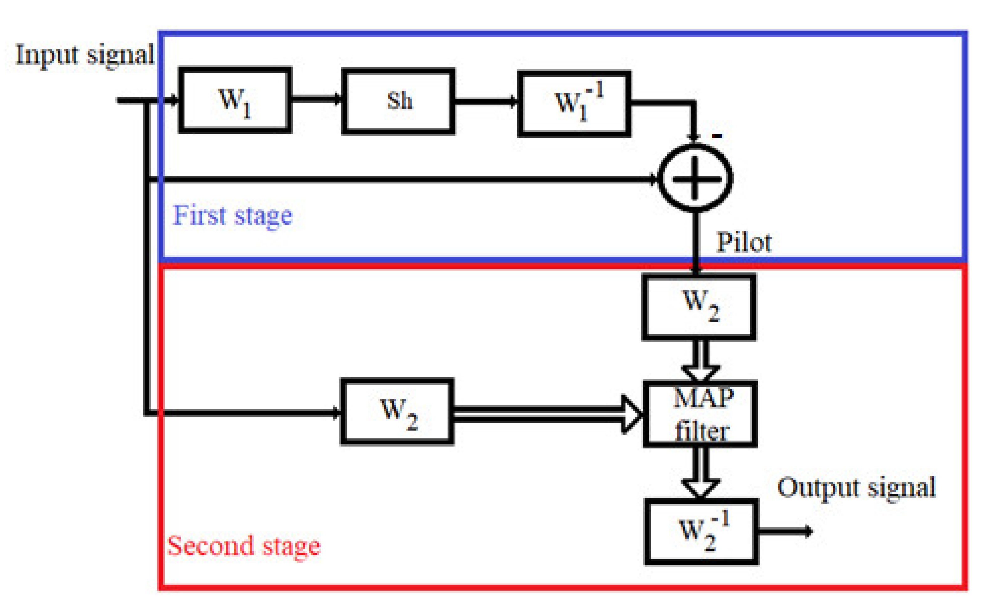
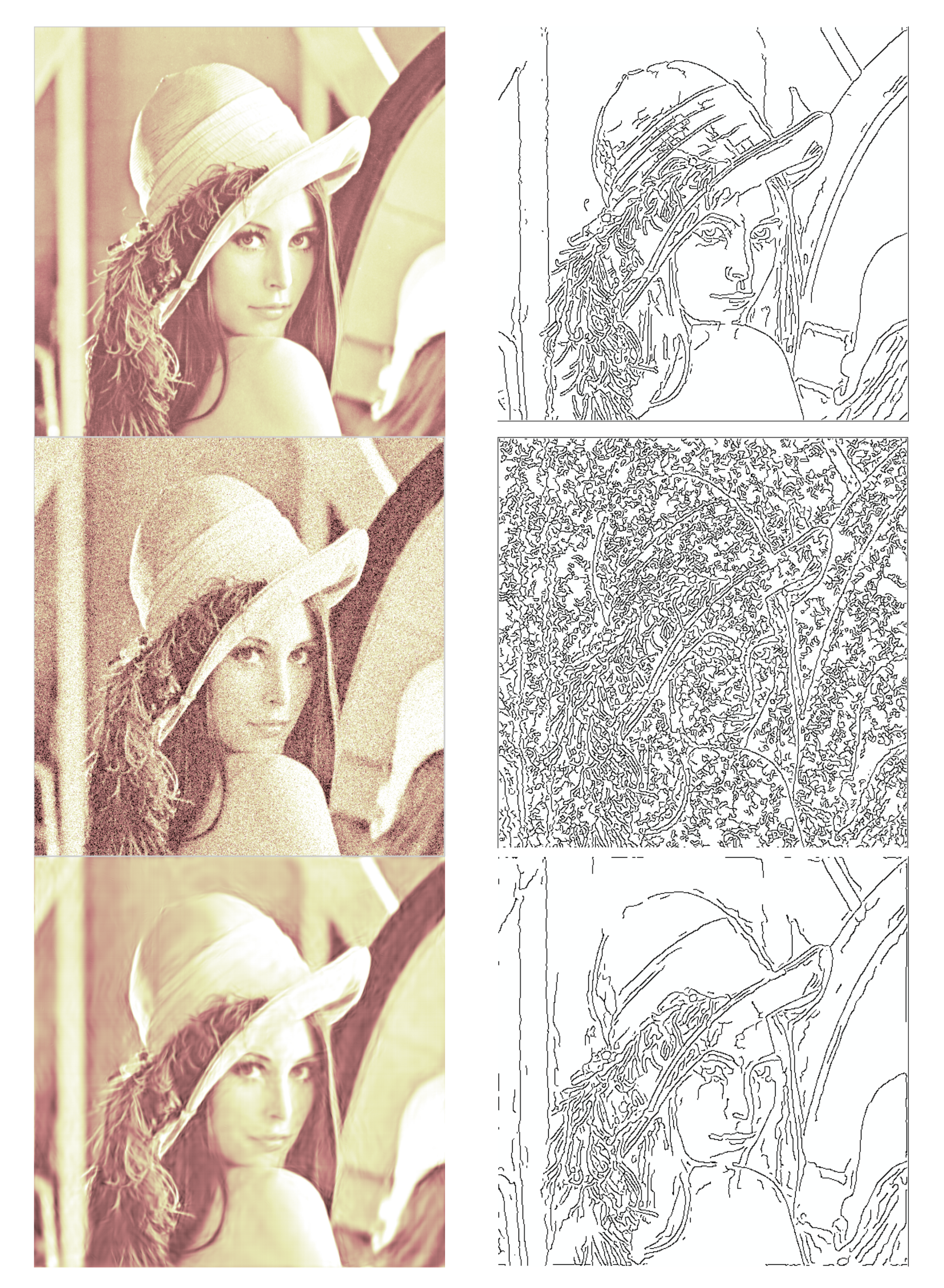
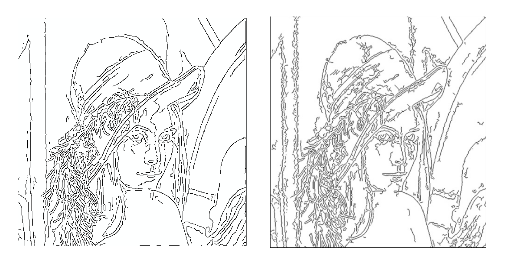
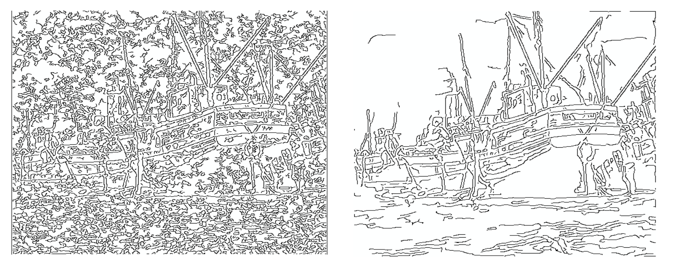
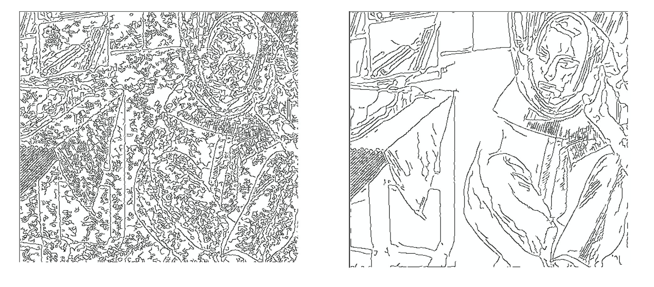
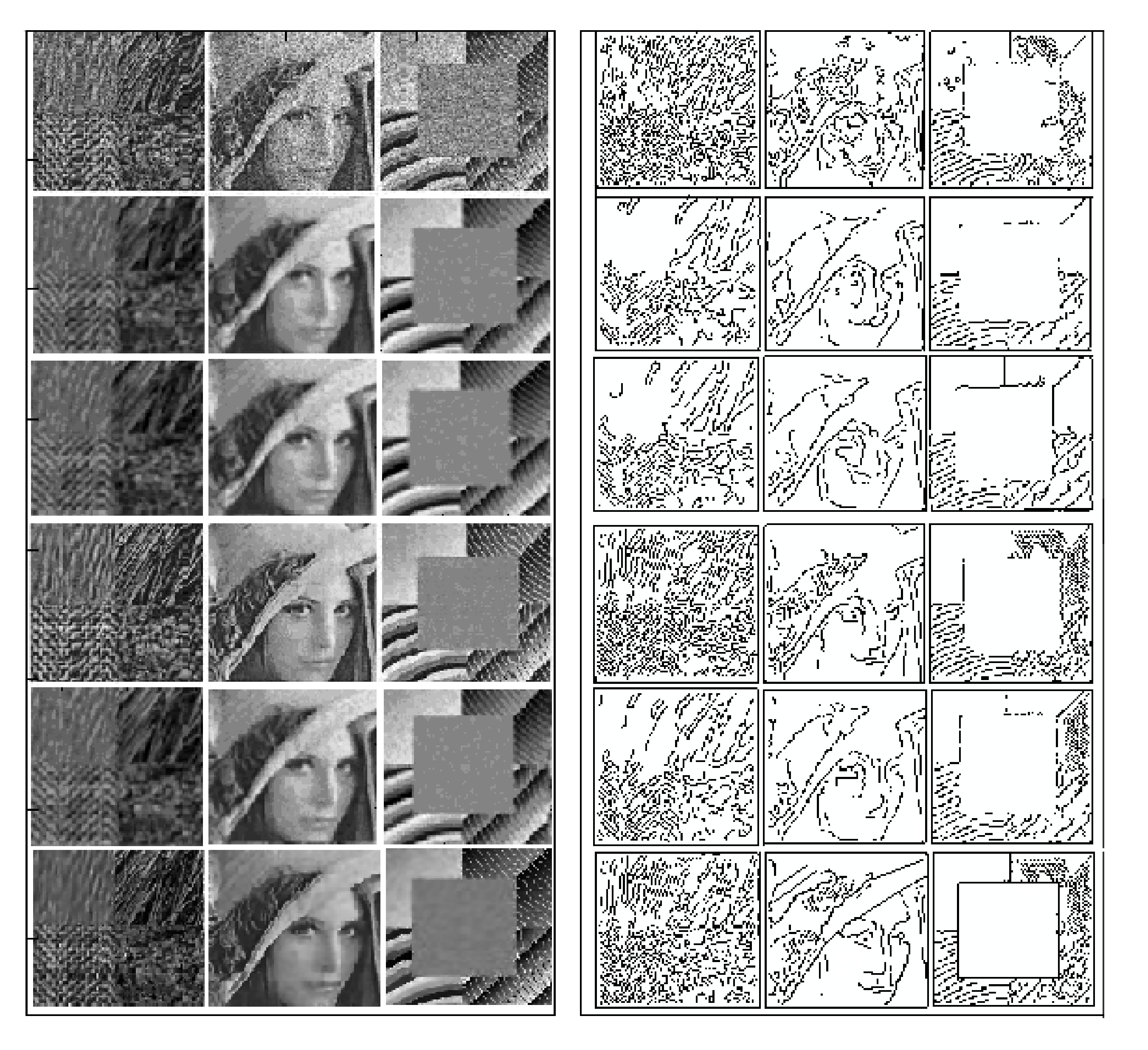
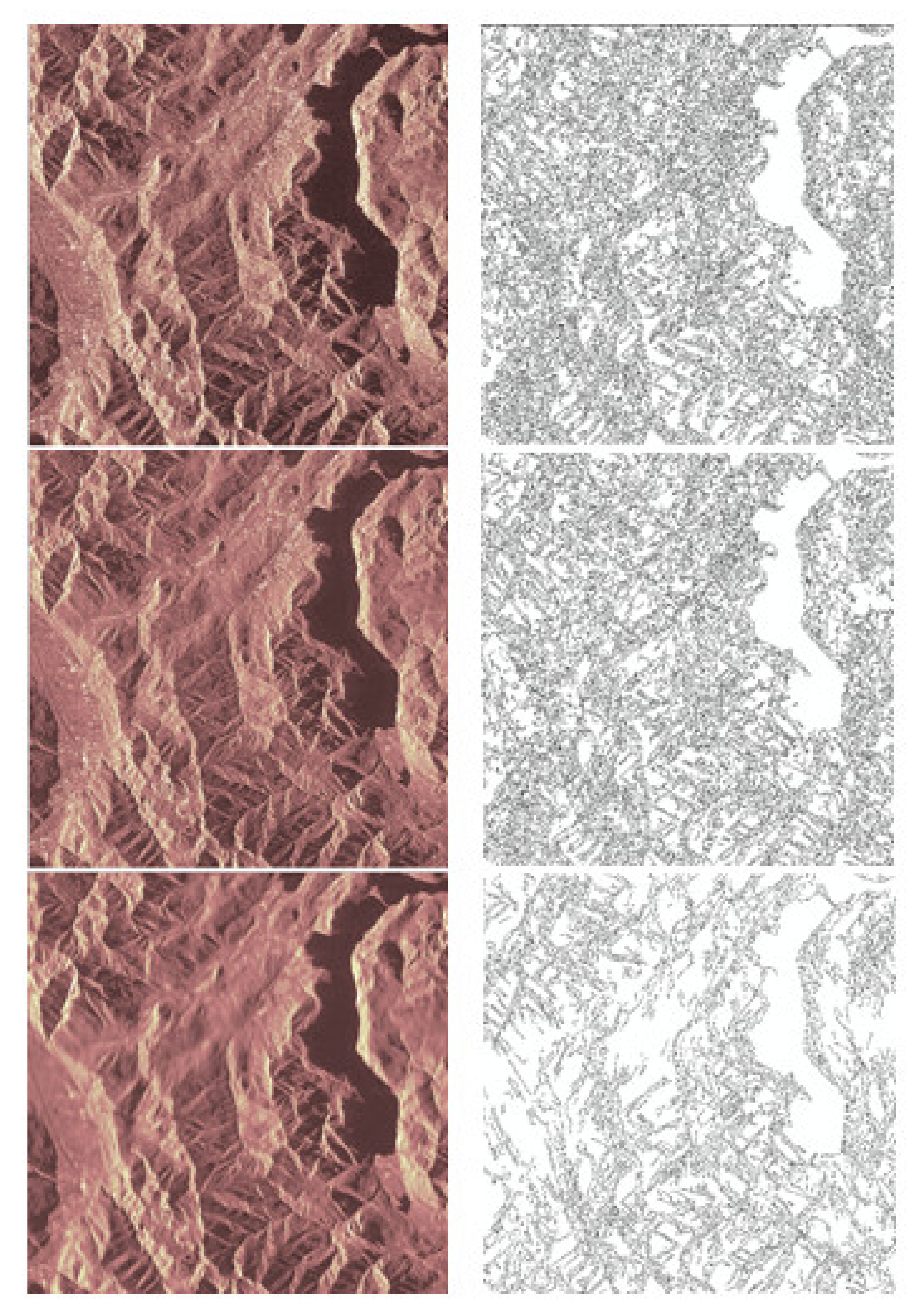
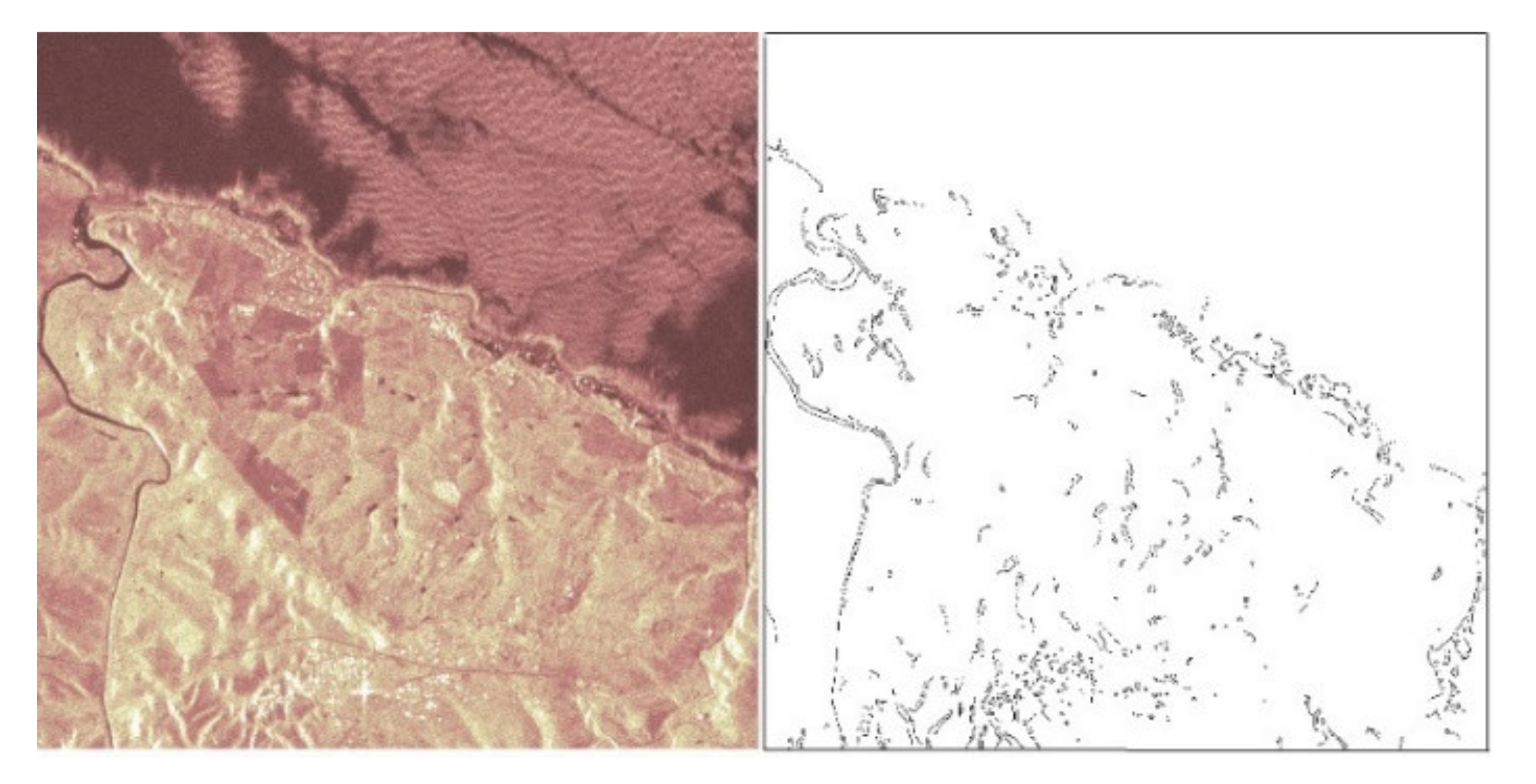
Table 1.
Image Lena. A comparison of the results obtained for the proposed method and for Canny’s edge detector applied directly on the noisy image, for different values of noise standard deviation.
Table 1.
Image Lena. A comparison of the results obtained for the proposed method and for Canny’s edge detector applied directly on the noisy image, for different values of noise standard deviation.
| Proposed Method | Canny’s Method | ||||
|---|---|---|---|---|---|
| First Step | Final Result | Directly on Noisy Image | |||
| Input PSNR | Output PSNR | Output SSIM | Edges’ MSE | Edges’ MSE | |
| 10 | 28.13 | 35.19 | 0.9989 | 0.04 | 0.07 |
| 15 | 24.59 | 33.41 | 0.9983 | 0.06 | 0.09 |
| 20 | 22.10 | 32.06 | 0.9977 | 0.07 | 0.14 |
| 25 | 20.21 | 31.06 | 0.9971 | 0.07 | 0.2 |
| 30 | 18.61 | 30.20 | 0.9964 | 0.08 | 0.21 |
Table 2.
Image Boat. A comparison of the results obtained for the proposed method and for Canny’s edge detector directly applied to the noisy image, for different values of the noise standard deviation.
Table 2.
Image Boat. A comparison of the results obtained for the proposed method and for Canny’s edge detector directly applied to the noisy image, for different values of the noise standard deviation.
| Proposed Method | Canny’s Method | ||||
|---|---|---|---|---|---|
| First Step | Final Result | Directly on Noisy Image | |||
| Input PSNR | Output PSNR | Output SSIM | Edges’ MSE/no. of missed pixels | Edges’ MSE/no. of false edge pixels | |
| 10 | 28.13 | 33.11 | 0.9981 | 0.05/1122 | 0.06/1218 |
| 15 | 24.59 | 31.20 | 0.9970 | 0.07/2828 | 0.09/5247 |
| 20 | 22.10 | 29.86 | 0.9959 | 0.09/5443 | 0.14/13,538 |
| 25 | 20.21 | 28.82 | 0.9948 | 0.1/6893 | 0.18/17,130 |
| 30 | 18.61 | 28.08 | 0.9935 | 0.1/6978 | 0.20/26,644 |
Table 3.
Image Barbara. A comparison of the results obtained for the proposed method and for Canny’s edge detector directly applied to the noisy image, for different values of the noise standard deviation.
Table 3.
Image Barbara. A comparison of the results obtained for the proposed method and for Canny’s edge detector directly applied to the noisy image, for different values of the noise standard deviation.
| Proposed Method | Canny’s Method | ||||
|---|---|---|---|---|---|
| First Step | Final Result | Directly on Noisy Image | |||
| Input PSNR | Output PSNR | Output SSIM | Edges’ MSE/no. of missed pixels | Edges’ MSE/no. of false edge pixels | |
| 10 | 28.13 | 33.23 | 0.9987 | 0.05/516 | 0.06/3672 |
| 15 | 24.59 | 31.31 | 0.9978 | 0.06/523 | 0.09/7995 |
| 20 | 22.10 | 29.41 | 0.9968 | 0.07/2052 | 0.14/16,922 |
| 25 | 20.21 | 28.21 | 0.9956 | 0.08/3235 | 0.17/25,815 |
| 30 | 18.61 | 27.06 | 0.9943 | 0.09/4335 | 0.2/29,272 |
Table 4.
Image Lena. PSNR [dB] performance of different wavelet-based despeckling systems: proposed in [48]; the association of HWT with a marginal ASTF [58]; the association of HWT with Bishrink filter, obtained using two different MWs: Daubechies 4 (D4) and Biorthogonal Daubechies 9/7 (B9/7).
| NL | Noisy | Result in [48] | HWT - | HWT - | |||
|---|---|---|---|---|---|---|---|
| Marginal ASTF | Bishrink | ||||||
| D4 | B9/7 | D4 | B9/7 | D4 | B9/7 | ||
| 1 | 12.1 | 26.0 | 26.2 | 25.4 | 25.6 | 25.7 | 26.2 |
| 4 | 17.8 | 29.3 | 29.6 | 29.9 | 30.0 | 29.9 | 30.4 |
| 16 | 23.7 | 32.9 | 33.1 | 33.2 | 32.9 | 33.0 | 33.3 |
Table 5.
Image Lena. PSNR [dB] performance of different despeckling systems: results reported in [49]: MAP-S; results reported in [53]: SA-WBMMAE, PPB, SAR-BM3D, H-BM3D; and results of proposed method.
| NL | Noisy | SA-WB MMAE | MAP-S | PPB | SAR-BM3D | H-BM3D | Prop. |
|---|---|---|---|---|---|---|---|
| 1 | 12.1 | 25.0 | 26.3 | 26.7 | 27.9 | 26.4 | 26.4 |
| 4 | 17.8 | 29.0 | 29.8 | 29.8 | 29.6 | 31.2 | 30.6 |
| 16 | 23.7 | 32.4 | 33.2 | 32.7 | 34.1 | 34.5 | 33.5 |
Table 6.
Comparison of components performance in the two-stage denoising system proposed in terms of ENL.
Table 6.
Comparison of components performance in the two-stage denoising system proposed in terms of ENL.
| Method | Parameters | |
|---|---|---|
| ENL | Noise Rejection | |
| Input image | 2 | Unavailable |
| First stage (HWT-marginal ASTF) | 3.4 | Worst result |
| Entire System | 7.61 | Best result |
Publisher’s Note: MDPI stays neutral with regard to jurisdictional claims in published maps and institutional affiliations. |
© 2021 by the authors. Licensee MDPI, Basel, Switzerland. This article is an open access article distributed under the terms and conditions of the Creative Commons Attribution (CC BY) license (https://creativecommons.org/licenses/by/4.0/).
Share and Cite
MDPI and ACS Style
Isar, A.; Nafornita, C.; Magu, G. Hyperanalytic Wavelet-Based Robust Edge Detection. Remote Sens. 2021, 13, 2888. https://0-doi-org.brum.beds.ac.uk/10.3390/rs13152888
AMA Style
Isar A, Nafornita C, Magu G. Hyperanalytic Wavelet-Based Robust Edge Detection. Remote Sensing. 2021; 13(15):2888. https://0-doi-org.brum.beds.ac.uk/10.3390/rs13152888
Chicago/Turabian StyleIsar, Alexandru, Corina Nafornita, and Georgiana Magu. 2021. "Hyperanalytic Wavelet-Based Robust Edge Detection" Remote Sensing 13, no. 15: 2888. https://0-doi-org.brum.beds.ac.uk/10.3390/rs13152888
Note that from the first issue of 2016, this journal uses article numbers instead of page numbers. See further details here.