SFRS-Net: A Cloud-Detection Method Based on Deep Convolutional Neural Networks for GF-1 Remote-Sensing Images

Abstract

Clouds constitute a major obstacle to the application of optical remote-sensing images as they destroy the continuity of the ground information in the images and reduce their utilization rate. Therefore, cloud detection has become an important preprocessing step for optical remote-sensing image applications. Due to the fact that the features of clouds in current cloud-detection methods are mostly manually interpreted and the information in remote-sensing images is complex, the accuracy and generalization of current cloud-detection methods are unsatisfactory. As cloud detection aims to extract cloud regions from the background, it can be regarded as a semantic segmentation problem. A cloud-detection method based on deep convolutional neural networks (DCNN)—that is, a spatial folding–unfolding remote-sensing network (SFRS-Net)—is introduced in the paper, and the reason for the inaccuracy of DCNN during cloud region segmentation and the concept of space folding/unfolding is presented. The backbone network of the proposed method adopts an encoder–decoder structure, in which the pooling operation in the encoder is replaced by a folding operation, and the upsampling operation in the decoder is replaced by an unfolding operation. As a result, the accuracy of cloud detection is improved, while the generalization is guaranteed. In the experiment, the multispectral data of the GaoFen-1 (GF-1) satellite is collected to form a dataset, and the overall accuracy (OA) of this method reaches 96.98%, which is a satisfactory result. This study aims to develop a method that is suitable for cloud detection and can complement other cloud-detection methods, providing a reference for researchers interested in cloud detection of remote-sensing images.

1. Introduction

With the rapid development of satellite remote-sensing technology, satellite remote-sensing images are playing an increasingly important role in the production and life of today’s society. Fields such as industry, agriculture, and the service industry cannot develop well without the support of satellite remote-sensing data [1,2,3,4,5]. However, according to the International Satellite Cloud Climatology Project flux data (ISCCP-FD), the global annual average cloud cover is estimated to be approximately 66% [6,7]. As the cloud obscures the ground information, a large amount of invalid data in remote-sensing images is produced, occupying too much storage space and transmission bandwidth. Besides this, cloud also has a huge impact on applications in the fields of earth resource exploration, natural disaster forecasting, and environmental pollution detection [8,9,10,11]. Although accurate cloud masks can be created by manual interpretation, the massive amount of remote-sensing data is obviously not suitable for this time-consuming manual operation. Therefore, accurate automatic cloud detection has become one of the problems that must be solved in the application of remote-sensing data.

As early as 1983, cloud-detection technology became an important part of the World Climate Research Program (WCRP) [12]. After long-term development, a series of research results regarding cloud-detection technology have been achieved. However, the complex information in remote-sensing images brings substantial challenges to cloud-detection technology and its generalization. Besides this, there are still unresolved problems in areas such as change detection, map making, and ground target recognition that require accurate cloud detection. According to the number of input images, cloud-detection methods can be divided into single-date methods and multitemporal methods [13,14]. Adding the feature of time, multitemporal cloud-detection methods identify the cloud by comparing the cloudy image with the clear-sky reference image, sharing relatively high detection accuracy. However, compared with single-date cloud-detection methods, multitemporal cloud-detection methods are more complicated to operate as they require clear sky reference images or high-density time series data, thus probably causing problems in monitoring land changes. This study mainly discusses the single-date cloud-detection method.

Generally speaking, for optical remote-sensing images, single-date cloud-detection methods mainly include physical methods using spectral reflectance characteristics, texture statistics methods, and machine-learning methods [15]. Specifically, the cloud-detection method using spectral reflection characteristics mainly focuses on the threshold to distinguish cloud and ground by the differences in the spectral reflection characteristics of cloud and ground. The texture statistics method generally determines the type of texture through the pattern and spatial distribution of the texture, to classify cloud and ground. The machine-learning method introduces technologies that can automatically learn features to realize the classifications of cloud and ground, of which the most representative type is deep learning (DL) technology [16,17,18].

As the spectral reflectance characteristics of the cloud and ground are different, the threshold methods such as the dual-spectral threshold method [19], multispectral threshold method [20], and dynamic threshold method [21,22], set the thresholds according to the differences in reflectivity, brightness, and temperature shown by cloud and ground in each band to achieve cloud detection. In 1977, Raynolds and Haar proposed a dual-spectral threshold detection method that mainly uses the visible band and infrared band for cloud detection [23]. Subsequently, the advanced very-high-resolution radar (AVHRR) sensor, which can acquire multiband remote-sensing data, was developed. In 1987, Saunders used a series of physical thresholds to process AVHRR sensor data for cloud detection [24]. Later, multiple bands of Landsat7 enhanced thematic mapper (ETM+) were used by automatic cloud coverage assessment (ACCA). Through the combination of the information of different bands, cloud mask products were obtained by using multiple thresholds [25,26]. The subsequent function of mask (Fmask) algorithm covered almost all the available band information in the Landsat series and Sentinel-2 satellite remote-sensing images. The Fmask algorithm is considered to be an upgrade version of ACCA [27,28,29]. The threshold method is easy to implement and relatively mature, yet it has some limitations in practical applications. First of all, the threshold is highly related to the data and the equipment that collects the data. The threshold method often fails when the collected images vary with the state of the equipment. Secondly, the threshold method is highly sensitive to the noise in the data, easily leading to false detection results. Finally, when the underlying surfaces are deserts, coastlines, snow, and ice that have similar reflectivity as clouds, detection errors will occur. Therefore, although the threshold method is simple and easy to implement, its detection accuracy and generalization cannot satisfy most accurate cloud-detection tasks.

As the resolution of remote-sensing images increases, the texture and spatial characteristics of remote-sensing images play an increasingly important role in cloud detection. The spatial information between pixels expresses the structural attributes and element relevance of the surface of an object, thus it is in line with the macroscopic observation results of human vision [30]. In 1988, Welch et al. developed features such as energy, entropy, contrast, and correlation from the gray-level co-occurrence matrix to express the texture characteristics of remote-sensing images [31]. In 2019, Pingfang Tian proposed a remote-sensing image cloud-detection method based on the variance of the fractal dimension [32]. Yihua Tan et al. employed a maximum response (MR) filter to extract the texture features of clouds in different directions and at different scales, obtaining eight-dimensional feature vectors [33]. Although the method extracts a large number of cloud texture features, it is time-consuming because of the large amount of calculation. Wavelet transform realizes the expression of texture features under multiscale conditions and improves the accuracy of cloud detection [34], yet the texture method also features large calculation, long time, and low efficiency. Moreover, texture features are mainly designed manually, and the selection of texture often depends on expert knowledge. The texture threshold requires repeated iterative tests, leading to high cost. Although these methods have made some progress, most of them are not adaptable enough. Excessive use of prior knowledge often leads to poor generalization in complex scenarios.

To avoid manual design and improve the generalization of cloud-detection algorithms, machine-learning techniques that can automatically learn features are applied to cloud-detection tasks [35,36], including clustering [37,38], artificial neural networks (ANN) [39,40], random forest (RF) [41,42], support vector machine (SVM) [43,44,45], DL [46,47,48,49,50,51], and the like. As computer hardware proceeds, cloud-detection algorithms based on DCNN have gradually become a research hotspot. In recent years, various DCNN have been developed by computer vision researchers. The first few layers of DCNN can extract local features, and the deep layers can extract large-area features, indicating that DCNN can automatically extract corresponding features at multiple levels. Compared with artificially extracted shallow features, DCNN shares better feature expression capability. Based on the U-Net structure, Jeppesen et al. presented the remote-sensing network (RS-Net) for cloud detection in remote-sensing images in 2019. [52]. The multiscale convolutional feature fusion (MSCFF) cloud-detection method, which integrates multiscale information into convolutional features, was proposed by Zhiwei Li et al. [53]. Though the DL method can automatically extract features through self-learning and minimize human intervention, its detection of the edge of complex cloud areas is not precise as pooling operations are inevitably implemented for multiple times in DL frameworks, as a result of diversified shapes and sizes of clouds. Therefore, for some tasks requiring high cloud-detection accuracy, the accuracy of cloud-detection technology based on DL needs to be improved.

The information in remote-sensing images is complex and the amount is huge. Various types of cloud, mountains, desert, cities, rivers, and other ground features often appear in the same remote-sensing image, posing challenges to the robustness and generalization ability of cloud-detection algorithms. The features in the threshold method and texture statistics method are designed manually, and then appropriate threshold ranges and texture combination categories are summarized through continuous experimental iterations. Therefore, the generalization ability of the threshold method and the texture statistics method is insufficient. In addition, the threshold method relies too much on the spectral information; for example, the ACCA algorithm suitable for AVHRR payload cannot be applied to satellites with only four spectral bands such as GF-1, GaoFen-2 (GF-2), and ZiYuan3-02 (ZY3-02). The texture statistical method requires a huge amount of calculation, and it is costly to obtain a suitable texture feature combination. In comparison, DL methods have excellent feature self-acquisition capabilities, and are well adaptable to remote-sensing images from various complex scenes. Moreover, the convolutional neural networks (CNN) solve the problem of excessive parameters, thus the DL technology based on CNN is suitable for cloud-detection tasks. However, the pooling layer used to extract high-level features in the DL framework blurs the details of the feature map, which is disadvantageous for accurate cloud-detection tasks. To apply DL to precise cloud-detection tasks, SFRS-Net is proposed, in which the traditional pooling layer is replaced by space folding, extracting high-level features while retaining as many details as possible.

As an earth-observation satellite featuring high spatial resolution, multispectrum and wide coverage, the GF-1 satellite is mainly adopted in the fields of resource survey, monitoring, supervision, emergency response, environmental protection, agriculture, forestry, marine, and the surveying and mapping industries. Its wide coverage ensures its coverage of more types of ground and cloud, and its high spatial resolution ensures its offering of more image details, providing convenience for cloud-detection research. Furthermore, its mission determines that accurate cloud detection is an essential data-processing step. Therefore, the optical remote-sensing images of the GF-1 satellite are selected in this study.

The rest of this paper is arranged as follows: The proposed methodology for cloud detection is explained in Section 2. The experimental results of the proposed method are presented in Section 3. Section 4 discusses the advantages, limitations, and applicability of the proposed method. Section 5 presents the conclusions and the direction of future work.

2. Methods

The SFRS-Net proposed in this study is a semantic segmentation network based on the encoder–decoder structure, as shown in Figure 1. The left/right part, called encoder/decoder, consists of a series of layers. The nodes in each layer are organized as three dimensions corresponding to the rows, columns, and channels of the feature map. The bottom layers on the left and right represent the input and output images, respectively, while the middle layers represent a series of middle feature maps. Before the final segmentation result is output, the input image undergoes a series of operations such as convolution, folding, and unfolding, from left to right. In the encoding part, the traditional pooling layers are replaced by folding layers; in the decoding part, the traditional upsampling layers are replaced by unfolding layers. The function of folding/unfolding is to retain as many details as possible during sampling/upsampling, so as to make the segmentation result more refined. The feature map in the encoder is directly transferred to the feature map of the corresponding size in the decoder through concatenation.

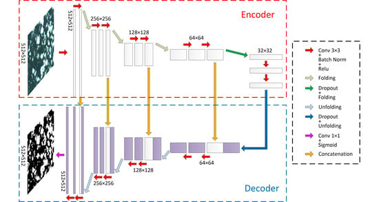
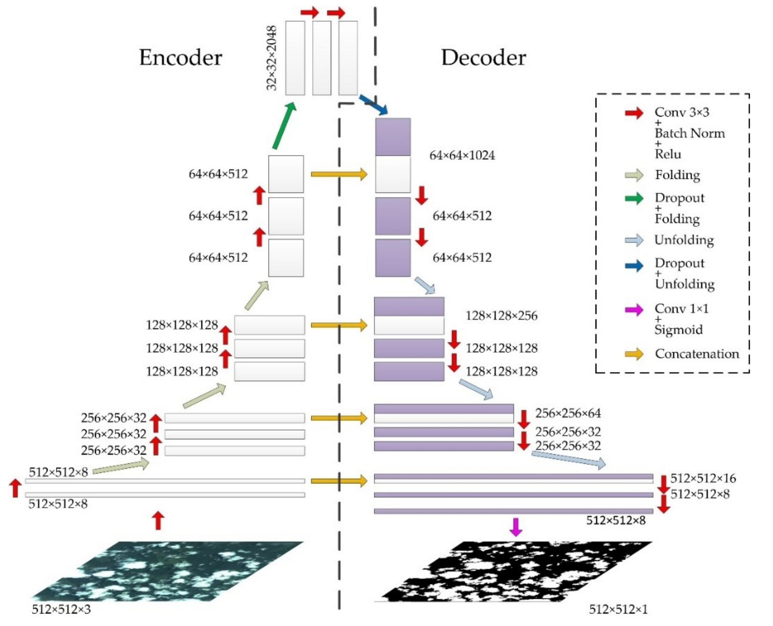
2.1. The SFRS-Net Architecture

In addition to the application of traditional technology, the SFRS-Net adopts a folding–unfolding operation.

2.1.1. Traditional Layers

As the most important part of DCNN, the convolutional layer is mainly used for feature extraction and fusion. It is assumed that X and W are the input feature map and convolutional kernel of the convolutional layer, the size of X is M × N × C (M, N, C are the height, width, and number of channels), and the size of W is m × n × C (m, n, and C are the height, width, and number of channels of the convolutional kernel). W_k and B_k are the k-th convolutional kernel and bias, and the output of the k-th feature map can be calculated by Equation (1):

$$y_{k,i,j}={\displaystyle \sum _{d=0}^{C-1}{\displaystyle \sum _{u=0}^{m-1}{\displaystyle \sum _{v=0}^{n-1}{W}_{k,d,u,v}\cdot x_{d,i+u,j+v}}}}+B_k$$

(1)

where the range of i is [0, M-m], and the range of j is [0, N-n].

The convolutional kernel is actually a weight matrix, which represents a way of dealing with the relationship between a pixel and its neighboring pixels. Generally speaking, the size of the convolutional kernel is proportional to the amount of calculation. When the convolutional kernel is large, the amount of calculation tends to increase greatly. At present, the most frequently used size of convolutional kernel is 3 × 3. The convolutional kernel could realize cross-channel interaction and information integration in multichannel neural networks, and easily increase/decrease the number of channels.

After the convolution operation, the size of the feature map output is inconsistent with that of the input one. The height and width of the output feature map of each convolutional layer is kept the same as the input one by filling zeros on the image boundary before the convolution operation.

According to Equation (1), the operation in the convolutional layer is linear. For the network to learn the characteristics of the image better, a nonlinear operation is introduced—that is, an activation function layer is added behind the convolutional layer; otherwise, no matter how many layers of the CNN has, the output is merely a linear combination of the inputs, limiting the approximation ability of the network. Therefore, the activation function layer is added to intensify the deep neural networks for better completion of cloud-detection tasks. The rectified linear unit (Relu) function is used as the activation function here, as shown in Equation (2).

$$f(x)=\max \left(x,0\right)$$

(2)

Compared with other functions, Relu features fast convergence as it only needs one threshold to obtain the activation value, dispensing with complicated calculations.

A batch normalization (BN) operation can readjust the response of the previous layer, as shown in Equations (3)–(6). A BN operation has two advantages. First, it can be used to adjust the network to reduce overfitting, which is especially important when the dataset is small. Secondly, it helps to increase the training speed, because the gradient is rescaled at each layer during back propagation.

$$\mu =\frac{1}{m}{\displaystyle \sum _{i=1}^m{x}_i}$$

(3)

$${\sigma }^2=\frac{1}{m}{\displaystyle \sum _{i=1}^m{\left(x_i-\mu \right)}^2}$$

(4)

$${\widehat{x}}_i=\frac{x_i-\mu }{\sqrt{{\sigma }^2+\tau }}$$

(5)

$$y_i={\widehat{x}}_i\cdot \gamma +\beta$$

(6)

where m is the number of pixels in the batch, $\mu$ the mean value of all the pixels, $\sigma$ the variance of all the pixels, $\tau$ a constant, ${\widehat{x}}_i$ the normalized pixel value, and $y_i$ the pixel value after transformation and reconstruction.

The direct function of dropout is to reduce the number of intermediate features, thereby reducing feature redundancy and increasing the orthogonality among features in each layer. Dropout is applied in the hidden layer. For a certain layer L, if dropout with probability p is applied, the neurons of this layer will be “dropped” with probability p during network training/testing, and the “dropped” neurons are no longer considered in the calculation of the weight matrix. A dropout operation could prevent the network from relying too much on a certain mode.

The loss function is adopted to estimate the degree of difference between the predicted value and the actual value. In DCNN, the loss function plays a vital role. The smaller the value of the loss function, the better the network performs. By minimizing the loss function, the model can reach a state of convergence, reducing the error of the model’s predicted value. In this study, the loss function is a measure of the degree of fitting between the segmentation result and the ground truth.

Loss function could be defined by several ways, such as mean square error, maximum likelihood estimation, maximum posterior probability, and cross-entropy loss function. Since the pixels in the image are divided into cloud pixels and noncloud pixels, a binary cross-entropy loss function is used, as shown in Equation (7).

$$Loss=-\left(p\times \log \left(\widehat{p}\right)+\left(1-p\right)\times \log \left(1-\widehat{p}\right)\right)$$

(7)

where, p is the pixel label (if the pixel is a cloud pixel, the value is 1; otherwise, the value is 0), and $\widehat{p}$ the probability that the pixel is predicted to be cloud.

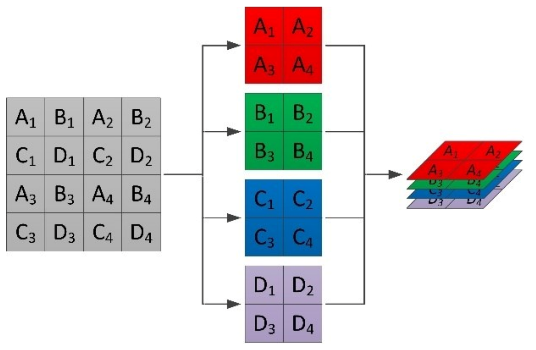
2.1.2. Folding Layer and Unfolding Layer

The pooling layer mainly used for downsampling is replaced by the folding layer in this study. Through continuous pooling, substantial characteristics could be acquired by the convolution operation. However, information missing is inevitable during the sampling process, and the discarded information often determines the details of image segmentation. In most cloud-detection tasks, the edge of the cloud needs to be accurately segmented, but the pooling layer brings an obstacle. Therefore, the pooling layer is replaced by the folding layer in this study to ensure that the overall characteristics are obtained without loss of local details.

In this study, a one-layer feature map is split into a four-layer one according to certain rules, then the new feature map becomes half of the previous one in width and height, yet it has four layers in the vertical space. It should be noted that the images in this study are not divided into four quadrants (each quadrant is distributed on a different layer) as artificial destruction is not allowed in the DCNN training process. The folding method is shown in Figure 2.

In Figure 2, A₁, B₁, C₁, and D₁ are extracted to form the first layer; A₂, B₂, C₂, and D₂ the second layer; A₃, B₃, C₃, and D₃ the third layer; and A₄, B₄, C₄, and D₄ the fourth layer. In this way, the feature mapping is transformed into four layers. Adjacent pixels are assigned to layers in different spaces according to the rule, which is equivalent to spatially folding adjacent pixels. Since detailed information is not discarded as the pooling layer does, through continuous folding, we can obtain the overall characteristics during the training process while retaining the detailed information to the greatest extent.

In order to explain the folding process more generally, the coordinates of a point in the L-th feature map are assumed to be (x, y), where x is the number of rows and y is the number of columns. After the folding operation, the new layer number $\widehat{L}$ of the point and the coordinates ($\widehat{x}$, $\widehat{y}$) can be calculated by Equations (8)–(10).

$$\widehat{x}=⌊x/2⌋$$

(8)

$$\widehat{y}=⌊y/2⌋$$

(9)

$$\widehat{L}=\left\{\begin{array}{cc} \hspace{1em}4\times L ,& if x \mathrm{mod} 2 = 0 and y \mathrm{mod} 2 = 0\hfill \\ 4\times L+1,& if x \mathrm{mod} 2 = 0 and y \mathrm{mod} 2 = 1\hfill \\ 4\times L+2,& if x \mathrm{mod} 2 = 1 and y \mathrm{mod} 2 = 0\hfill \\ 4\times L+3,& if x \mathrm{mod} 2 = 1 and y \mathrm{mod} 2 = 1\hfill \end{array}\right.$$

(10)

Analysis and extraction of feature information is completed in the encoding stage. In the decoding stage, the parsed information needs to be mapped to specific pixels. Since the traditional upsampling method predicts the pixel value to be added through calculation, the multilayer upsampling operation cannot meet the accuracy requirements. Therefore, the traditional upsampling method is replaced by the unfolding layer to retain information, which is to be recovered gradually through the unfolding layer, increasing image detail information. The unfolding layer corresponding to the folding layer is used in the decoding stage, and the folding layer is used in the encoding stage. Unfolding is the reverse operation of folding, as presented in Figure 3.

In Figure 3, A₁, B₁, C₁, and D₁ are extracted from the first layer; A₂, B₂, C₂, and D₂ from the second layer; A₃, B₃, C₃, and D₃ the third layer; and A₄, B₄, C₄, and D₄ the fourth layer. Reverse operation (unfolding) against folding is then carried out to restore the four-layer feature map to a one-layer feature map.

In order to explain the unfolding process more generally, the coordinates of a point in the L-th feature map are assumed to be (x, y), where x is the number of rows and y is the number of columns. After the unfolding operation, the new layer number $\widehat{L}$ of the point and the coordinates ($\widehat{x}$, $\widehat{y}$) can be calculated by Equations (11)–(13).

$$\widehat{L}=⌊L/4⌋$$

(11)

$$\widehat{x}=\left\{\begin{array}{cc}2\times x ,& if L \mathrm{mod} 4 = 0 or L \mathrm{mod} 4 = 1\hfill \\ 2\times x+1,& if L \mathrm{mod} 4 = 2 or L \mathrm{mod} 4 = 3\hfill \end{array}\right.$$

(12)

$$\widehat{y}=\left\{\begin{array}{cc}2\times y ,& ifL \mathrm{mod} 4 = 0 or L \mathrm{mod} 4 = 2\hfill \\ 2\times y+1,& if L \mathrm{mod} 4 = 1 or L \mathrm{mod} 4 = 3\hfill \end{array}\right.$$

(13)

2.2. Data Preprocessing

Since the image is calculated layer by layer in the DCNN, the storage space occupied by DCNN increases sharply when input image increases. As the remote-sensing image is usually large in size (the multispectral image of GF-1 has a width of 4548 pixels and a height of 4503 pixels), it is almost impossible to process a whole remote-sensing image at a time on a device with limited graphics processing memory. The fully convolutional networks (FCN) [16] technology used in the proposed method does not limit the size of the image. Therefore, to maintain a low memory consumption during training, each remote-sensing image (including its corresponding ground truth) was divided into a series of small nonoverlapping images, with the size of 512 × 512. The resolution of the GF-1 multispectral image is 8 m. The observation area of a 512 × 512 image is 1,677,216 square meters, containing most of the ground features. As a 1024 × 1024 image is too large for our device memory, and a 256 × 256 image has such a limited observation area that certain mountainous terrain features cannot be included in one image, the 512 × 512 image was finally selected. These images were divided into three sets: the training set, the validation set, and the test set. Totals of 70%, 10%, and 20%, respectively, of the images were randomly grouped into the three sets, as shown in

Table 1. Training, evaluation, and test set statistics.

	Image (512 × 512)
	Training	Validation	Test
Amount	7441	1063	2126
Percentage	70%	10%	20%

. According to literature [54], the ratio of images used for training and testing is 4 : 1. The validation set is used for parameter adjustment during training. According to the literature [47], the size of the validation set should be 1/10 of the whole dataset. Therefore, the percentages were set as 70%, 10%, and 20%, respectively. The training set was used to train DCNN, the validation set was used for parameter adjustment, and the test set was only adopted for the final evaluation.

2.3. Implementation and Training

During implementation and training, the remote-sensing data is enlarged by rotating the images (including the ground truth) 90°, 180°, and 270° clockwise and flipping the resulting images up and down. Because these processed images are treated as new images by the model, the dataset was expanded by eight times. Finally, the data-set was divided into the training set, validation set, and test set. To obtain a robust model that is not sensitive to feature types, at least one representative sample of each feature type should be included in the training and verification process. Although images of any size could be input, fixed-size images are finally selected for simplicity.

The structure of the proposed network is the encoder–decoder structure. The shallow coding layer extracts detailed local features, and as the coding layer deepens, the overall characteristics can be acquired. Narrowing the length and width of the feature map, the folding layer acts as a downsampler. The decoder reconstructs the feature map through the unfolding layer that acts as an upsampler. The convolutional layer in the decoder is frequently used to recover detailed semantic features. Equal-sized feature mappings in the encoder and decoder are connected by concatenation, adding more spatial details in the reconstructed feature map generated in the decoder. The closer a feature map is to the output layer, the higher the level of semantic features it contains. These semantic features are often critical and tend to contribute substantially to the output of the network.

In the study, Tensorflow 1.12.0 and the Keras API python package were used for network training by the method of stochastic gradient descent (SGD). The learning rate decay strategy was set to be “cosine annealing”. The maximum learning rate was 0.1 and the minimum learning rate was 0. The momentum parameter was set as 0.9, the size of training batch 4, and the number of training iterations 1000. An Adam optimizer with default parameter settings was employed. The network training was supported by NVIDIA GeForce RTX 1080Ti.

3. Results

3.1. Dataset

In the process of selecting data, the possible impacts of the varieties of geographical location and climate environment on the algorithm should be considered, thus the images selected should be diversified. This study adopts the multispectral data of the GF-1 satellite. Collected from http://www.cresda.com/ (accessed on 1 July 2020), the data in this study is composed of four bands, and the resolution is 8 m. The data characteristics are shown in

Table 2. Technical indicators of the GF-1 satellite payload.

Spectral Band No.	Spectral Name	Spectral Range (μm)	Spatial Resolution (m)
Band1	Blue	0.45–0.52	8
Band2	Green	0.52–0.59	8
Band3	Red	0.63–0.69	8
Band4	Near Infrared(NIR)	0.77–0.89	8

. The dataset contains 10,630 GF-1 images, with a size of 512 × 512. Among them, the training set contains 7441 images, the verification set 1063, and the test set 2126. These images were shot from May 2019 to March 2020. To establish the dataset, we first transformed the GF-1 images into true RGB 24-bit color images, which were then classified into different types of terrain [1,55], such as city, mountain, water, ice, desert, vegetation, and comprehensive terrain. City images include 1595 scenes, mountain images 1062 scenes, water images 1063 scenes, ice images 1065 scenes, desert images 1060 scenes, vegetation images 2126 scenes, and comprehensive terrain images 2658 scenes. In each case, 70% of the images constitute the training set, 10% the validation set, and 20% the test set. The training set, validation set, and test set contain multiple terrains to maximize the diversity. Each piece of scene data in the dataset is equipped with a corresponding artificially labeled ground truth. The original images were transformed into true RGB 24-bit color images, which were then labeled as cloud and ground by the Adobe Photoshop software. The true RGB images were used for visual inspection. The ground truths were manually checked by five operators, who would vote for determination of controversial areas. The results were decided by the majority vote. The ground truths were evaluated by five other analysts. The margin of error was 6.3% compared with the previous results. Figure 4 shows the difference of the ground truth manually labeled by different operators.

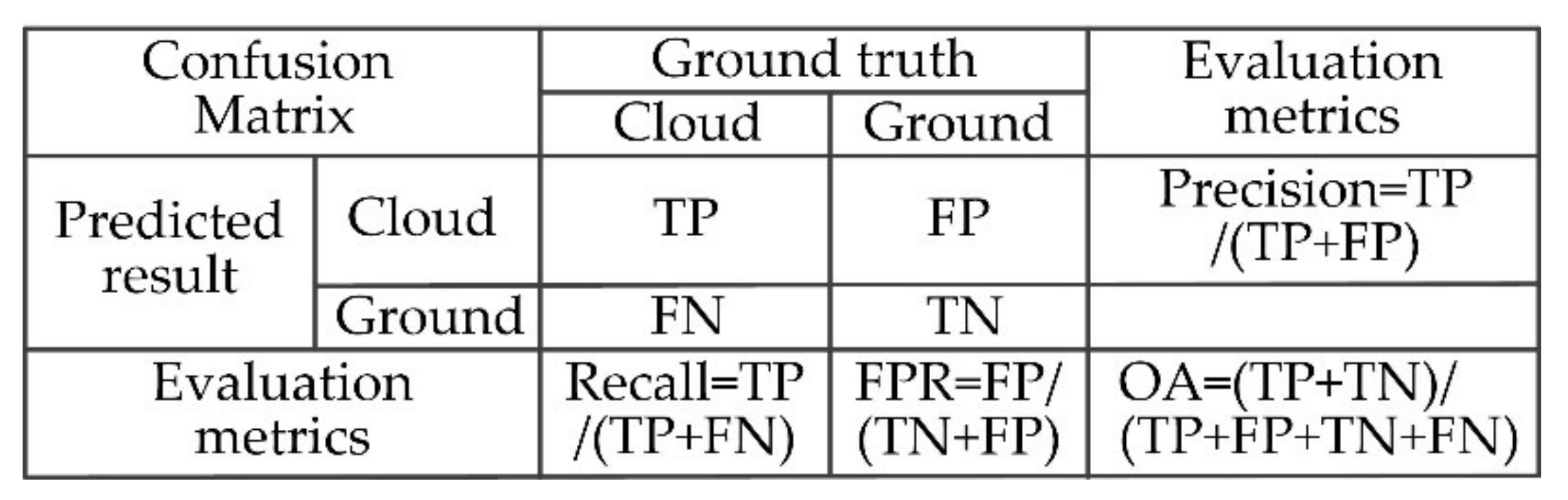
3.2. Evaluation Criteria

Such commonly used benchmark metrics as precision, recall, false positive rate (FPR), and OA are used to evaluate the performance of cloud-detection algorithms. The four types of test results are defined as: (1) The number of pixels that are correctly detected as cloud: True Positive (TP); (2) The number of pixels that are correctly detected as ground: True Negative (TN); (3) The number of pixels that are incorrectly detected as cloud: False Positive (FP); and (4) False Negative (FN): the number of pixels that falsely detect the cloud as ground. According to the four types of detection results, the metrics for evaluating the performance of cloud-detection algorithms can be obtained, as shown in Equations (14)–(17), and the hybrid matrix is shown in Figure 5:

$$Precision=TP/\left(TP+FP\right)$$

(14)

$$Recall=TP/\left(TP+FN\right)$$

(15)

$$FPR=FP/\left(TN+FP\right)$$

(16)

$$OA=\left(TP+TN\right)/\left(TP+TN+FP+FN\right)$$

(17)

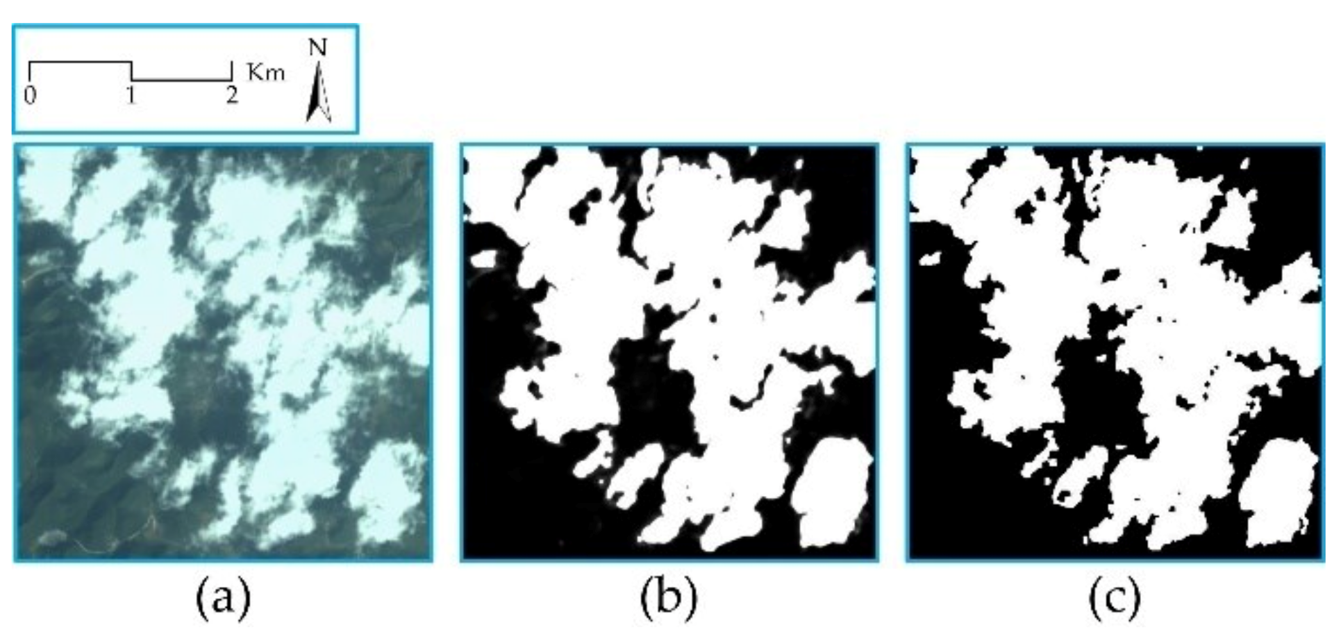
3.3. Validity of the Folding–Unfolding Method

Figure 6 presents the comparison results of folding/unfolding operations, and pooling and traditional upsampling methods. Image (a) is the original image, (b) the cloud-detection result by the method of max-pooling and upsampling, and (c) the cloud-detection result by the method of folding/unfolding operations. Through comparison, it can be observed that the detection results of folding/unfolding operations are more detailed on the cloud edge than those of the max-pooling and upsampling methods, and the irregular lines of the cloud edge are better presented. The results uncover that folding–unfolding operations could retain more image information, thus scoring high accuracy in cloud detection.

Table 3. Assessment of the detection results by folding–unfolding and pooling on the test set.

	Precision%	Recall%	FPR%	OA%
Pooling	96.74	95.80	3.95	95.91
Folding–unfolding	97.17	97.35	3.47	96.98

shows the statistical cloud-detection results of the folding–unfolding method and the pooling operation on the test set. It can be seen from Table 3 that the folding–unfolding method scores better in detection results.

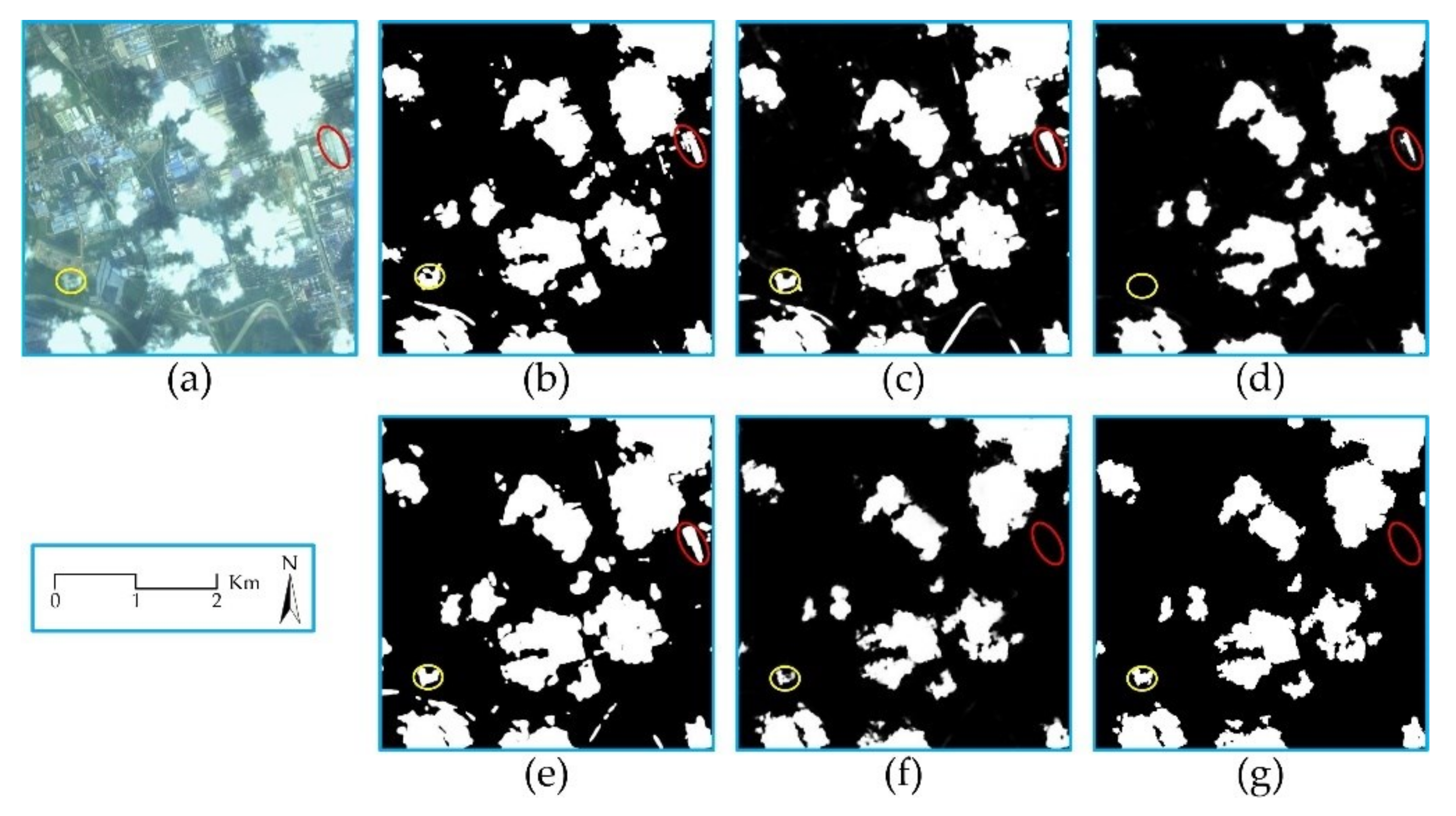
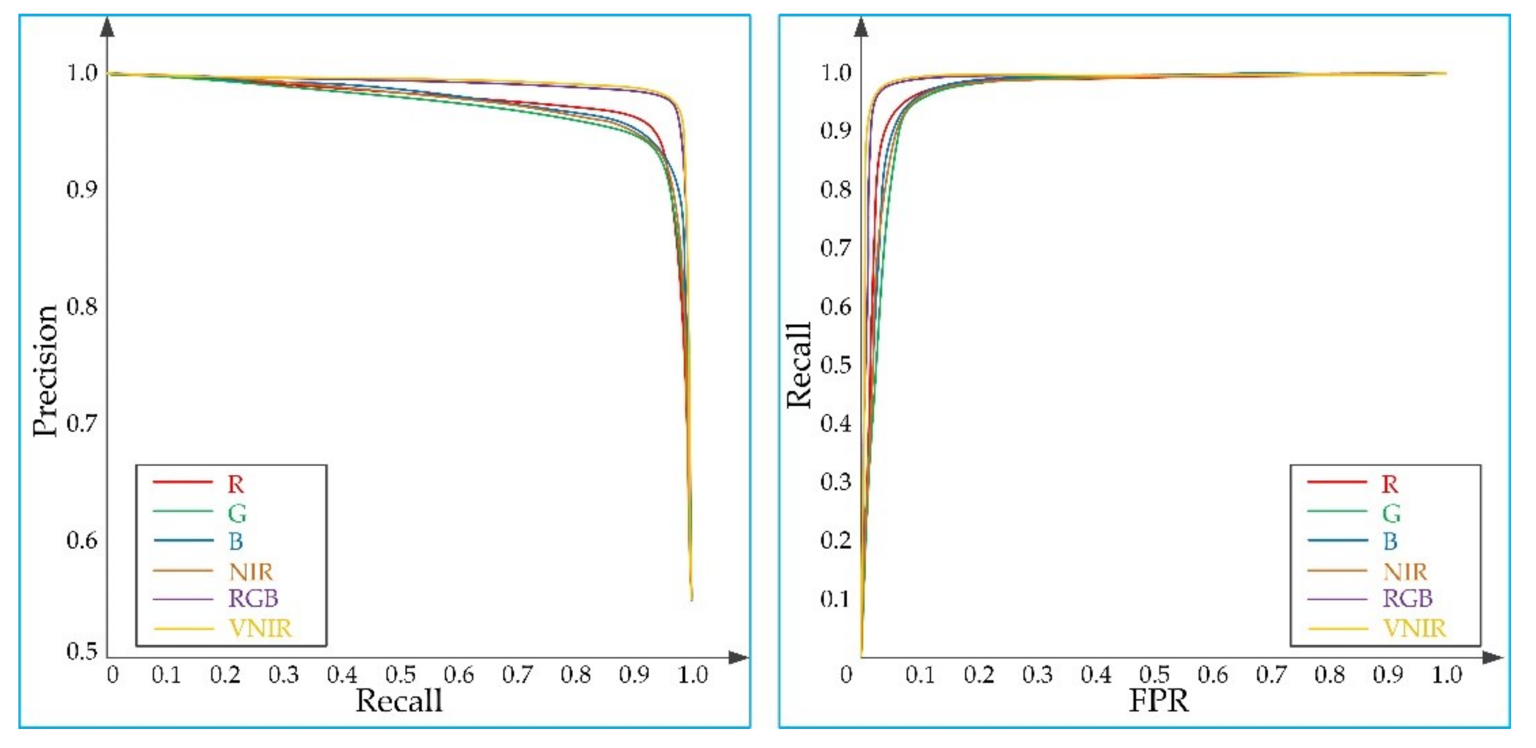
3.4. Comparative Experiment of Different Bands

The influence of different bands and band combinations on cloud-detection results was analyzed. In Figure 7, (a) represents the original RGB image (with cloud regions of complex edges and random shapes), (b) the cloud-detection result in the B band, (c) the cloud-detection result in the G band, (d) the cloud-detection result in the R band, (e) the cloud-detection result in the NIR band, (f) the RGB cloud-detection result, and (g) the visible and near-infrared (VNIR) cloud-detection result. As shown in the red ellipse in Figure 7, the R band, the G band, the B band, and NIR band show that this is a cloud area, while RGB bands and VNIR bands show that this is a noncloud area. According to the original image, the area in the red ellipse is actually a noncloud area. Besides this, the area in the yellow ellipse is labeled as a noncloud area by the R band, while the G-band and B band, NIR band, RGB bands, and VNIR bands show otherwise. According to the original image, it is identified that the area in the yellow ellipse is a cloud area. Although the cloud region can be correctly detected on both RGB and VNIR images, the VNIR image records the optimal cloud-detection results, which can also be verified by

Table 4. Assessment of the detection results under different bands on the test set.

	B	G	R	NIR	RGB	VNIR
Precision%	94.38	93.80	95.79	94.17	97.13	97.17
Recall%	92.84	93.15	91.80	92.63	97.29	97.35
FPR%	6.76	7.52	4.93	7.01	3.51	3.47
OA%	93.02	92.85	93.27	92.79	96.93	96.98

(the VNIR image records the highest value of OA). It can be seen visually that the cloud-detection results of multiband images are better than those of single-band images, revealing the importance of band information for cloud detection. The statistical results are shown in Table 4, and the precision–recall (PR) curve and the receiver operator characteristic (ROC) curve in Figure 8. In Table 4, B denotes the blue band, G the green band, R the red band, NIR the NIR band, RGB the true color image, and VNIR the VNIR bands.

In Table 4, the precision value of the VNIR bands are the highest, indicating that the real cloud pixels in the VNIR bands account for the highest proportion of the detected cloud pixels. The recall value of VNIR bands is the highest, indicating that the cloud pixels detected correctly in VNIR bands account for the highest proportion in the real cloud pixels. The FPR value of the VNIR bands is the lowest, indicating that the pixel of the ground judged as cloud is the least on the VNIR bands. The OA value of VNIR bands is the highest, indicating that all correctly detected pixels account for the highest proportion in the total pixel. In Table 4, the higher the values of recall, precision, and OA, the better the detection results; the smaller the value of FPR, the fewer the commission errors. In the PR curve in Figure 8, the closer the curve is to the upper right, the higher the detection accuracy of the cloud area; in the ROC curve, the closer the curve is to the upper left, the more the cloud is detected, the less the commission errors, and the higher the detection accuracy.

The cloud-detection results of the VNIR image are shown in Figure 9. The original images and the detection results are placed side by side, and the details are marked in the same positions of the two images. Figure 9a shows the cloud-detection results of vegetation, cities, ice, and snow, (b) water and bare land, and (c) villages, crops, and a large number of translucent clouds. It can be identified from the detailed images that (a) and (b) contain high reflectivity features, and the boundary between the cloud and the ground in (c) is obscure as some ground objects are blurred by the cloud, reducing the observation value. It can be seen from the details in Figure 9 and Table 4 that the proposed method shows a favorable cloud-detection effect.

A total of 500 GF-1 images from other time periods (July 2020 to September 2020) were collected. The cloud-detection results of the data collected during other time periods by the proposed method in

Table 5. Assessment of the detection results under additional images.

	Precision%	Recall%	FPR%	OA%
Additional image	97.05	97.08	3.61	96.77

indicate that the images collected during other time periods can also be effectively detected by the proposed method.

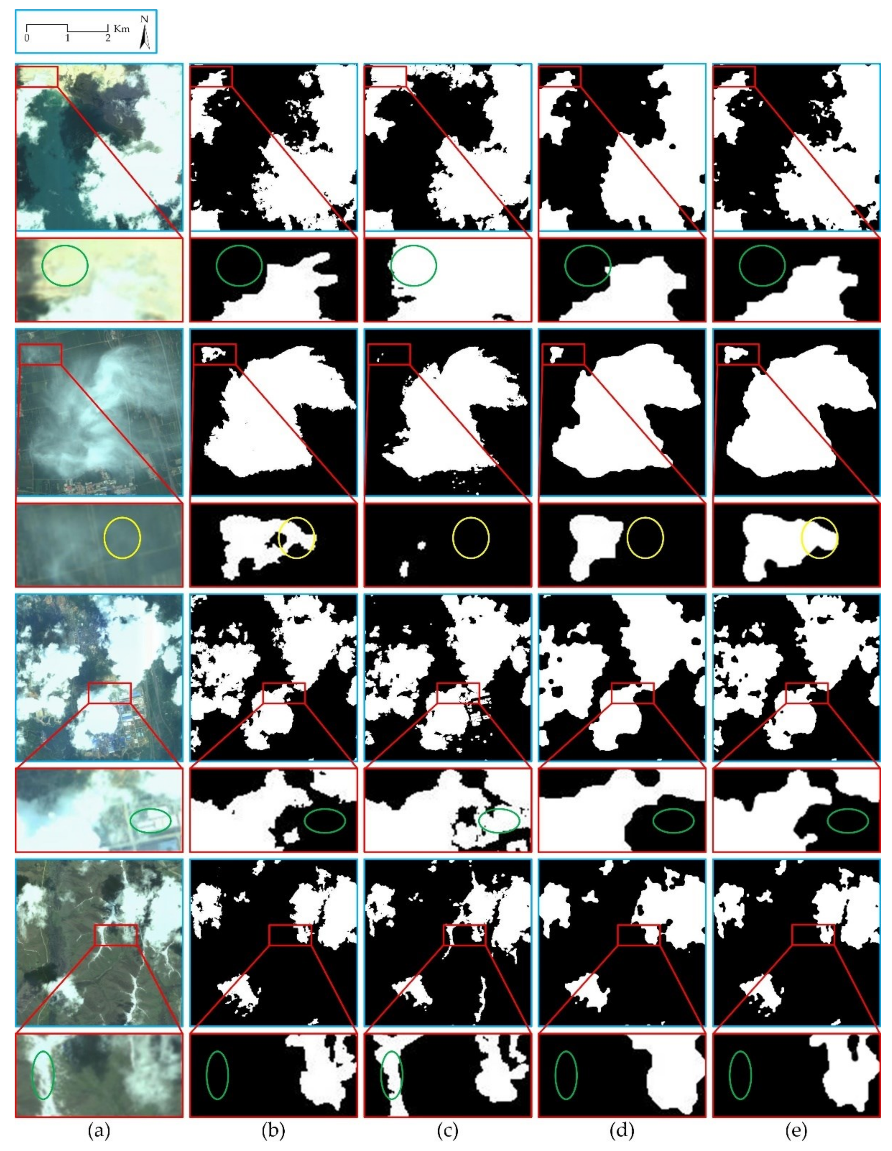
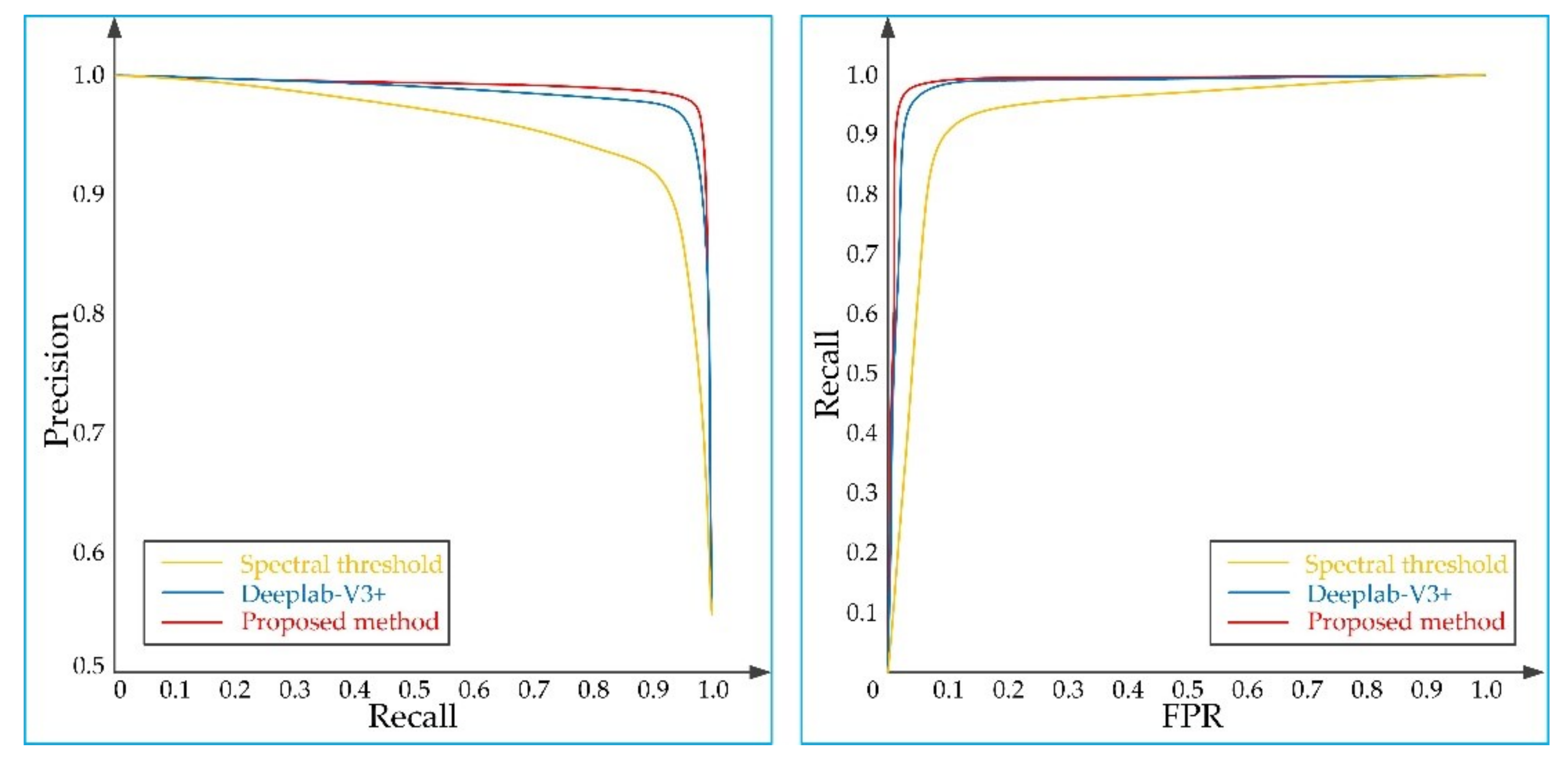
3.5. Comparative Experiment of Different Methods

The detection performance of the proposed method, the spectral threshold method and Deeplab-V3+ is compared using the same dataset on the same hardware platform. This study mainly compares the cloud masks generated by the three methods (Figure 10).

In Figure 10, the first column is the original image, the second column the ground truth, the third column the detection result of the spectral threshold method, the fourth column the detection result of the Deeplab-V3+, and the fifth column the detection result of the proposed method. It can be identified that the cloud edges in the detection results of the spectral threshold method are the most complex and sharp among the counterparts, followed by the detection results of the proposed method, and finally the detection results of Deeplab-V3+. However, the false-detection phenomenon appears in cities and icy areas by the spectral threshold method, while commission errors are well-controlled by the proposed method and Deeplab-V3+. When the cloud is relatively thin, the ground spectrum will be mixed with the cloud spectrum, causing omission errors by the spectral threshold method. The scenes in Figure 10 were selected from the test set. The types of terrain described above are included in Figure 10. The first row presents desert and water, the second vegetation, the third city, and the fourth mountain and ice. The scenes shown in Figure 10 represent the types of terrain in the test set. The results of different methods on the test set are displayed in

Table 6. Assessment of the detection results by different methods in VNIR bands.

Method	Evaluation Metrics	Vegetation	Mountain	Water	City	Desert	Snow/Ice	Entire Test Set
The spectral threshold method	Precision%	96.71	95.94	97.09	94.68	85.86	78.72	92.36
	Recall%	94.94	96.42	92.71	93.37	89.30	81.99	89.37
	FPR%	4.84	5.75	4.63	6.82	12.03	20.05	9.03
	OA%	95.03	95.52	93.71	93.29	88.57	80.92	90.09
Deeplab-V3+	Precision%	97.95	97.78	97.32	96.37	92.61	89.81	96.07
	Recall%	98.41	97.98	95.56	96.23	95.08	93.13	96.23
	FPR%	3.09	3.13	4.39	4.71	6.21	9.56	4.81
	OA%	97.81	97.52	95.58	95.82	94.37	91.72	95.76
The proposed method	Precision%	98.68	98.78	97.45	96.89	93.97	91.35	97.17
	Recall%	98.50	98.81	96.99	97.22	95.75	93.74	97.35
	FPR%	1.98	1.72	4.23	4.05	5.12	8.03	3.47
	OA%	98.31	98.59	96.53	96.67	95.27	92.81	96.98

.

Most of the cloud in the remote-sensing images can be detected by the three methods. However, it can be seen from the detection results that the proposed method ranks top among the three in terms of commission errors and omission errors. Displaying the detection results of these methods in the local details, the detailed local images uncover that the proposed method is the least vulnerable to commission errors and omission errors compared with the other methods, corresponding well to the actual ground truth.

To evaluate the detection results of the spectral threshold method, Deeplab-V3+ and the proposed method, the precision, recall, FPR, and OA of the three methods are compared and presented in Table 6.

From the results in Table 6, it can be seen that the proposed method is superior to the spectral threshold method and Deeplab-V3+ in precision, recall, FPR, and OA. The PR and ROC curves of the three methods are displayed in Figure 11. In the test set, the precision value of the proposed method is the highest, indicating that the proportion of real cloud pixels in cloud pixels detected by the proposed method is the highest. The recall value of the proposed method is the highest, indicating that the correct cloud pixels detected by the proposed method account for the highest proportion of all real pixels. The FPR value of the proposed method is the lowest, indicating that pixels of the ground that are judged as cloud by the proposed method are the least. The OA value of the proposed method is the highest, indicating that all correctly detected pixels account for the highest proportion in the total pixels. In Table 6, the higher the values of recall, precision, and OA, the better the detection results; the smaller the value of FPR, the fewer the commission errors. In the PR curve in Figure 11, the closer the curve is to the upper right, the higher the detection accuracy of cloud area; in the ROC curve, the closer the curve is to the upper left, the more the cloud is detected, the less the commission errors, and the higher the detection accuracy. According to the visual assessment of analysts, the OA value of 95% can be considered as a successful implementation of cloud detection.

4. Discussion

4.1. The Effectiveness of the Convolutional Network

Compared with other neural network structures, the CNN architecture is more suitable for processing images, because its input and hidden layer structure consists of three-dimensional (width, height, and depth) neuron layers that are well-adapted to multichannel image data processing. At the same time, the neurons in each layer are only connected to a small area of the layer before convolution by means of weight sharing, reducing the number of parameters and enlarging the possibility of DCNN to process large image data. In the CNN, the convolution operation is mainly used to extract features [56]. Compared with traditional image segmentation methods, DL methods based on CNN can obtain high-level semantic features such as texture and scene. Finally, each pixel in the image is assigned a category to form the desired segmentation result. During the actual cloud-detection tasks, the DCNN learns the clouded and nonclouded areas in the input images in advance according to the ground truth, achieving its robustness to complex cloud conditions. DCNN is conducive to extracting deep semantic features, improving the distinguishability of features similar to cloud in the underlying surface, realizing classification of each pixel in the input image. Finally, a segmentation mask with the same size as the input image is obtained and accurate segmentation of the cloud area is achieved.

4.2. The Effectiveness of the Folding–Unfolding Operation

Playing a vital role in DCNN, the pooling layer reduces the resolution of feature maps [57] to obtain high-level features. However, every time the feature image is pooled, part of the information in the image, especially the local detailed information, will be lost, impeding the creation of accurate cloud masks. As shown in Figure 12, compared with the ground truth, the edges of cloud regions detected by traditional DL are not accurate enough. In contrast, the folding layer could conduct downsampling on the feature maps without information lapse. The new feature map generated by extracted information is placed under the layer—that is, the single-layer planar feature map is converted into corresponding spatial four-layer feature map, retaining the local detailed information and laying the foundation for information recovery in the decoding stage. It should be noted that after each folding, the number of layers of the feature image will be four times as many as in the original layer, thus the number of convolutional kernels should be adjusted. In the decoding stage, the upsampling operation is replaced by the unfolding layer. The existing upsampling techniques generally estimate the filled pixels and calculate the corresponding information, instead of filling with existing real pixels. Taking another way to achieve upsampling, the unfolding layer gradually recovers the feature map to the size of the input image. Every time the recovery is achieved, the adjacent four-layer feature maps form a new feature map the length and width of which are twice the previous one according to specific rules. The new feature map is a combination of existing feature maps, and calculation and estimation are excluded. Therefore, the feature map generated by the unfolding layer will contain more real information, facilitating the recovery of the details of the feature maps in the decoding stage. It should be noted that after each unfolding, the number of layers of the feature image will become a quarter of the original layer, thus the number of convolutional kernels should be adjusted.

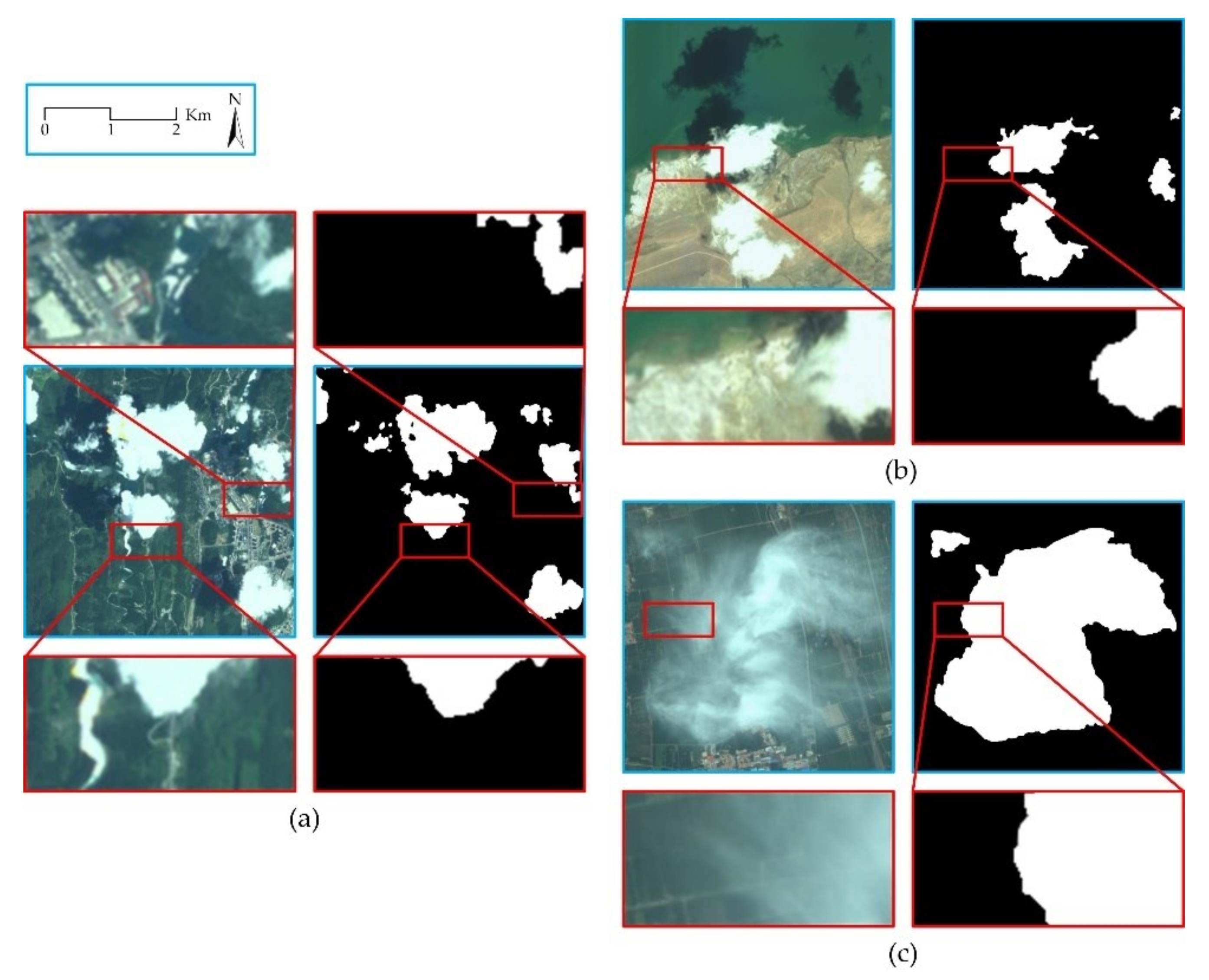
4.3. Error Sources of the Proposed Method

It can be concluded from the previous experiments that the proposed method records favorable cloud-detection results. Yet omission errors and commission errors may occur. Depending on the altitude of the sun and the shooting angle of the satellite, the shadow of some clouds may be cast on another part of the cloud, causing the missing detection (omission errors) of the cloud in the shadow. One reason for the omission errors is that the cloud obscured by the shadow shows a big difference from the normal cloud, resembling a noncloud area. The second reason is that cloud-area labeling is rather difficult in this case, and the accuracy of labeling is vulnerable to subjective factors, thus images should be marked by the same interpreter to reduce subjective errors. The ground truths are evaluated by different analysts. The margin of error is 6.3%. At the same time, it should be noted that cloud shadows on the ground will also weaken the spatial information of the ground, reducing image usability. Large-area highly reflective objects, such as ice and snow, can easily cause false detection (commission errors), because large-area highly reflective objects and the cloud are easily to be confused. To solve this problem, the depth of the model should be enlarged through hardware supports. In Figure 13, green ellipses in images mark omission errors, and red ellipses mark commission errors.

4.4. Influencing Factors of the Proposed Method

Since the proposed method is data-driven, the quality of the data directly affects the segmentation performance. An important factor that affects the segmentation results of our proposed method is image annotation. It should be emphasized that the ground truths for training, verification, and testing are obtained through manual interpretation and digitization of satellite images [53]. Therefore, the ground truths presented in this research are vulnerable to human analysts—that is, they are not absolute basic facts. In particular, the edge of cloud is usually obscure, as the boundary between cloud and ground is an obscure transition zone, thus relevant interpretation and depiction are not absolutely objective. Another factor that affects the proposed method is the quality of remote-sensing images. During data screening, the quality of images should be controlled strictly; for example, remote-sensing images with false shadows, missing bands, or overexposure cannot be selected. Since the training samples used in this study are limited, they may not be representative of all the types of cloud and ground. As it is not clear whether the trained model is adaptable to all the land observation satellite data, more training data regarding varying cloud and ground should be collected for verification.

4.5. Research and Application of the Proposed Method in the Future

The application of the proposed method to large-area bright surface objects (ice, snow) needs further research and improvement; for example, the number of ice and snow images could be increased in the training set, and geographic information processing functions could be added to the algorithm. As the satellite hardware technology proceeds, the onboard processing platform and communication among satellites will be improved. The satellite-borne cloud-detection technology could provide necessary cloud condition information for satellite groups, improving the efficiency of satellite group shooting, and reducing data transmission pressure. In the future, the proposed method will be further refined and simplified to prepare for the realization of accurate satellite-borne cloud-detection technology.

5. Conclusions

Since the multispectral images collected by the GF-1 satellite have only four spectral bands: blue, green, red, and NIR, the limitation of the number of spectral bands makes cloud detection a rather challenging problem. Generally speaking, traditional rule-based cloud-detection methods perform well in low- and medium-resolution images, because these images usually bear relatively rich spectral information. However, as the image spatial resolution increases and the available spectral bands reduce, coupled with the complexity of image information, it is difficult to accurately describe the target features, leading to decline of cloud-detection accuracy. This study thus proposes the SFRS-Net, a DCNN based on an encoder–decoder structure, in which the information of remote-sensing image features is extracted by the encoder (as the network deepens, overall and deep-level features can be extracted), and the local details are recovered by the decoder according to deep-level information, achieving pixel level segmentation. The above experiments show that this study only adopts the VNIR spectrum. Since satellites are designed for different purposes, not all the satellites are endowed with the same multispectral capabilities as the Landsat8 satellite; therefore, this study is of particular significance for satellites with limited spectral bands, especially low-cost nanosatellites.

This study presents folding layers and unfolding layers, in which the folding layer is used in the encoder part to replace the pooling layer for down-sampling. Unlike the pooling layer, the folding layer avoids local detail loss and saves information in a suitable way, laying foundation for the decoder to recover local details. Aiming to recover image details, the unfolding layer is used in the decoder part to replace the traditional upsampling operation. The folding layer and unfolding layer frequently appear in pairs, enhancing the network’s cloud area segmentation accuracy. The value of OA indicates the overall accuracy of the cloud-detection result. On the test set, the OA value of the proposed method is 6.89% higher than that of the spectral threshold method, and 1.12% higher than deeplabv3+, reaching 96.98%. Accurate cloud detection is achieved.

Cloud shadows weaken the ground information and reduce the availability of remote-sensing images, thus future study should also deal with cloud shadow detection. Besides, the structure of the proposed method should be further explored, such as the introduction method of geographic information and the improvement of computational efficiency, to optimize its performance and generalization ability.

References

1. Li, H.; Zheng, H.; Han, C.; Wang, H.; Miao, M. Onboard spectral and spatial cloud detection for hyperspectral remote sensing images. Remote Sens. 2018, 10, 152. [Google Scholar] [CrossRef] [Green Version]
2. Li, X.; Zheng, H.; Han, C.; Wang, H.; Zheng, W. Cloud detection of superview-1 remote sensing images based on genetic reinforcement learning. Remote Sens. 2020, 12, 3190. [Google Scholar] [CrossRef]
3. Jia, K.; Liang, S.; Gu, X.; Baret, F.; Wei, X.; Wang, X.; Yao, Y.; Yang, L.; Li, Y. Fractional vegetation cover estimation algorithm for Chinese GF-1 wide field view data. Remote Sens. Environ. 2016, 177, 184–191. [Google Scholar] [CrossRef]
4. Mercury, M.; Green, R.; Hook, S.; Oaida, B.; Wu, W.; Gunderson, A.; Chodas, M. Global cloud cover for assessment of optical satellite observation opportunities: A HyspIRI case study. Remote Sens. Environ. 2012, 126, 62–71. [Google Scholar] [CrossRef]
5. Shi, T.; Xu, Q.; Zou, Z.; Shi, Z. Automatic Raft Labeling for Remote Sensing Images via Dual-Scale Homogeneous Convolutional Neural Network. Remote Sens. 2018, 10, 1130. [Google Scholar] [CrossRef] [Green Version]
6. Rossow, W.; Duenas, E. The International Satellite Cloud Climatology Project (ISCCP) Web site—An online resource for research. Bull. Am. Meteorol. Soc. 2016, 85, 167–172. [Google Scholar] [CrossRef]
7. Zhang, Y.; Rossow, W.B.; Lacis, A.A.; Oinas, V.; Mishchenko, M.I. Calculation of radiative fluxes from the surface to top of atmosphere based on ISCCP and other global data sets: Refinements of the radiative transfer model and the input data. J. Geophys. Res. 2004, 109, 19105. [Google Scholar] [CrossRef] [Green Version]
8. Yuan, F.; Bauer, M.E. Comparison of impervious surface area and normalized difference vegetation index as indicators of surface urban heat island effects in Landsat imagery. Remote Sens. Environ. 2006, 106, 375–386. [Google Scholar] [CrossRef]
9. Shahbaz, M.; Lean, H.H. Does financial development increase energy consumption? The role of industrialization and urbanization in Tunisia. Energy Policy 2012, 40, 473–479. [Google Scholar] [CrossRef] [Green Version]
10. Superczynski, S.D.; Christopher, S.A. Exploring land use and land cover effects on air quality in Central Alabama using GIS and remote sensing. Remote Sens. 2011, 3, 2552. [Google Scholar] [CrossRef] [Green Version]
11. Dong, Q.; Yue, C. Image Fusion and Quality Assessment of GF-1. For. Inventory Planning 2016, 41, 1–5. [Google Scholar] [CrossRef]
12. Kotarba, A.Z. Evaluation of ISCCP cloud amount with MODIS observations. Atmos. Res. 2015, 153, 310–317. [Google Scholar] [CrossRef]
13. Wang, B.; Ono, A.; Muramatsu, K. Automated detection and removal of clouds and their shadows from Landsat tm images. Ice Trans. Inf. Syst. 1999, 82, 453–460. [Google Scholar] [CrossRef]
14. Udelhoven, T.; Frantz, D.; Schmidt, M. Enhancing the detectability of clouds and their shadows in multitemporal dryland Landsat imagery: Extending Fmask. IEEE Geosci. Remote Sens. Lett. 2015, 12, 1242–1246. [Google Scholar] [CrossRef]
15. Xiong, Q.; Wang, Y.; Liu, D.; Ye, S.; Zhang, X. A cloud detection approach based on hybrid multispectral features with dynamic thresholds for GF-1 remote sensing images. Remote Sens. 2020, 12, 450. [Google Scholar] [CrossRef] [Green Version]
16. Long, J.; Shelhamer, E.; Darrell, T. Fully convolutional networks for semantic segmentation. IEEE Trans. Pattern Anal. Mach. Intell. 2014, 39, 640–651. [Google Scholar] [CrossRef]
17. Badrinarayanan, V.; Kendall, A.; Cipolla, R. Segnet: A deep convolutional encoder-decoder architecture for image segmentation. IEEE Trans. Pattern Anal. Mach. Intell. 2017, 39, 2481–2495. [Google Scholar] [CrossRef]
18. He, K.; Gkioxari, G.; Dollar, P.; Girshick, R. Mask r-cnn. IEEE Trans. Pattern Anal. Mach. Intell. 2018, 42, 386–397. [Google Scholar] [CrossRef]
19. Xue, Q.; Guan, L. A Cloud Detection Method Combining ATMS Measurements and CrIS Hyperspectral Infrared Data at Double Bands. In Proceedings of the 2019 International Conference on Meteorology Observations (ICMO), Chengdu, China, 28–31 December 2019. [Google Scholar] [CrossRef]
20. Vittorio, A.; Emery, W.J. An automated, dynamic threshold cloud-masking algorithm for daytime AVHRR images over land. IEEE Trans. Geosci. Remote Sens. 2002, 40, 1682–1694. [Google Scholar] [CrossRef]
21. Liu, J. Improvement of dynamic threshold value extraction technic in fy-2 cloud detection. J. Infrared Millim. Waves 2010, 29, 288–292. [Google Scholar] [CrossRef]
22. Ma, F.; Zhang, Q.; Guo, N. The study of cloud detection with multi-channel data of satellite. Chin. J. Atmos. Sci. 2007, 31, 119–128. [Google Scholar] [CrossRef]
23. Reynolds, D.W.; Haar, T.H.V. A bi-spectral method for cloud parameter determination. Mon. Weather. Rev. 1977, 105, 446–457. [Google Scholar] [CrossRef] [Green Version]
24. Saunders, R.W.; Kriebel, K.T. An improved method for detecting clear sky and cloudy radiances from AVHRR data. Int. J. Remote Sens. 1988, 9, 123–150. [Google Scholar] [CrossRef]
25. Irish, R.R.; Barker, J.L.; Goward, S.N.; Arvidson, T. Characterization of the Landsat-7 ETM+ automated cloud-cover assessment (ACCA) algorithm. Photogramm. Eng. Remote Sens. 2006, 72, 1179–1188. [Google Scholar] [CrossRef]
26. Irish, R.R. Landsat 7 automatic cloud cover assessment. In Algorithms for Multispectral, Hyperspectral, and Ultraspectral Imagery VI; Shen, S.S., Descour, M.R., Eds.; International Society for Optics and Photonics: Bellingham, WA, USA, 2000; Volume 4049, pp. 348–356. [Google Scholar] [CrossRef]
27. Zhu, Z.; Woodcock, C.E. Object-based cloud and cloud shadow detection in Landsat imagery. Remote Sens. Environ. 2012, 118, 83–94. [Google Scholar] [CrossRef]
28. Zhu, Z.; Wang, S.; Woodcock, C.E. Improvement and expansion of the Fmask algorithm: Cloud, cloud shadow, and snow detection for Landsats 4–7, 8, and Sentinel 2 images. Remote Sens. Environ. 2015, 159, 269–277. [Google Scholar] [CrossRef]
29. Qiu, S.; Zhu, Z.; He, B. Fmask 4.0: Improved cloud and cloud shadow detection in Landsats 4–8 and Sentinel-2 imagery. Remote Sens. Environ. 2019, 231, 111205. [Google Scholar] [CrossRef]
30. Cai, Y.; Fu, D. Cloud recognition method and software design based on texture features of satellite remote sensing images. Trans. Atmos. Sci. 1999, 22, 416–422. [Google Scholar] [CrossRef]
31. Welch, R.M.; Sengupta, S.K.; Chen, D.W. Cloud field classification based upon high-spatial resolution textural feature, 1.Gray-level co-occurrence matrix approach. J. Geophys. Res. 1988, 93, 12663–12681. [Google Scholar] [CrossRef]
32. Tian, P.; Guang, Q.; Liu, X. Cloud detection from visual band of satellite image based on variance of fractal dimension. J. Syst. Eng. Electron. 2019, 30, 485–491. [Google Scholar] [CrossRef]
33. Tan, Y.; Ji, Q.; Ren, F. Real-time cloud detection in high resolution images using Maximum Response Filter and Principle Component Analysis. In Proceedings of the IGARSS 2016—2016 IEEE International Geoscience and Remote Sensing Symposium, Beijing, China, 10–15 July 2016; pp. 6537–6540. [Google Scholar] [CrossRef]
34. Mallat, S.G. A theory for multiresolution signal decomposition: The wavelet representation. IEEE Trans. Pattern Anal. Mach. Intell. 1989, 11, 674–693. [Google Scholar] [CrossRef] [Green Version]
35. Bai, T.; Li, D.; Sun, K.; Chen, Y.; Li, W. Cloud detection for high-resolution satellite imagery using machine learning and multi-feature fusion. Remote Sens. 2016, 8, 715. [Google Scholar] [CrossRef] [Green Version]
36. Tan, K.; Zhang, Y.; Tong, X. Cloud extraction from Chinese high resolution satellite imagery by probabilistic latent semantic analysis and object-based machine learning. Remote Sens. 2016, 8, 963. [Google Scholar] [CrossRef] [Green Version]
37. Gómez-Chova, L.; Camps-Valls, G.; Amoros-Lopez, J.; Guanter, L.; Alonso, L.; Calpe, J.; Moreno, J. New cloud detection algorithm for multispectral and hyperspectral images: Application to ENVISAT/MERIS and PROBA/CHRIS sensors. In Proceedings of the 2006 IEEE International Geoscience and Remote Sensing Symposium, Denver, CO, USA, 31 July–4 August 2006; pp. 2746–2749. [Google Scholar] [CrossRef]
38. Yu, W.; Cao, X.; Xu, L.; Bencherkei, M. Automatic cloud detection for remote sensing image. Chin. J. Sci. Instrum. 2006, 27, 2184–2186. [Google Scholar] [CrossRef]
39. Wieland, M.; Li, Y.; Martinis, S. Multi-sensor cloud and cloud shadow segmentation with a convolutional neural network. Remote Sens. Environ. 2019, 230, 111203. [Google Scholar] [CrossRef]
40. Chen, N.; Li, W.; Gatebe, C.; Tanikawa, T.; Hori, M.; Shimada, R.; Aoki, T.; Stamnes, K. New neural network cloud mask algorithm based on radiative transfer simulations. Remote Sens. Environ. 2018, 219, 62–71. [Google Scholar] [CrossRef] [Green Version]
41. Wei, J.; Huang, W.; Li, Z.; Sun, L.; Zhu, X.; Yuan, Q.; Liu, L.; Cribb, M. Cloud detection for landsat imagery by combining the random forest and superpixels extracted via energy-driven sampling segmentation approaches. Remote Sens. Environ. 2020, 248, 112005. [Google Scholar] [CrossRef]
42. Fu, H.; Shen, Y.; Liu, J.; He, G.; Chen, J.; Liu, P.; Qian, J.; Li, J. Cloud detection for FY meteorology satellite based on ensemble thresholds and random forests approach. Remote Sens. 2019, 11, 44. [Google Scholar] [CrossRef] [Green Version]
43. Joshi, P.P.; Wynne, R.H.; Thomas, V.A. Cloud detection algorithm using SVM with SWIR2 and tasseled cap applied to Landsat 8. Int. J. Appl. Earth Obs. Geoinform. 2019, 82, 101898. [Google Scholar] [CrossRef]
44. Li, P.; Dong, L.; Xiao, H.; Xu, M. A cloud image detection method based on SVM vector machine. Neurocomputing 2015, 169, 34–42. [Google Scholar] [CrossRef]
45. Ishida, H.; Oishi, Y.; Morita, K.; Moriwaki, K.; Nakajima, T.Y. Development of a support vector machine based cloud detection method for MODIS with the adjustability to various conditions. Remote Sens. Environ. 2018, 205, 390–407. [Google Scholar] [CrossRef]
46. Xie, F.; Shi, M.; Shi, Z.; Yin, J.; Zhao, D. Multilevel cloud detection in remote sensing images based on deep learning. IEEE J. Sel. Top. Appl. Earth Obs. Remote Sens. 2017, 10, 3631–3640. [Google Scholar] [CrossRef]
47. Chai, D.; Newsam, S.; Zhang, H.K.; Qiu, Y.; Huang, J. Cloud and cloud shadow detection in Landsat imagery based on deep convolutional neural networks. Remote Sens. Environ. 2019, 225, 307–316. [Google Scholar] [CrossRef]
48. Yang, J.; Guo, J.; Yue, H.; Liu, Z.; Hu, H.; Li, K. CDnet: CNN-based cloud detection for remote sensing imagery. IEEE Trans. Geosci. Remote Sens 2019, 57, 8. [Google Scholar] [CrossRef]
49. Guo, J.; Yang, J.; Yue, H.; Tan, H.; Li, K. CDnetv2: CNN-based cloud detection for remote sensing imagery with cloud-snow coexistence. IEEE Trans. Geosci. Remote Sens. 2020, 59, 1. [Google Scholar] [CrossRef]
50. Mateo-García, G.; Laparra, V.; López-Puigdollers, D.; Gómez-Chova, L. Transferring deep learning models for cloud detection between Landsat-8 and Proba-V. ISPRS J. Photogramm. Remote Sens. 2020, 160, 1–17. [Google Scholar] [CrossRef]
51. Mendili, L.E.; Puissant, A.; Chougrad, M.; Sebari, I. Towards a Multi-Temporal Deep Learning Approach for Mapping Urban Fabric Using Sentinel 2 Images. Remote Sens. 2020, 12, 423. [Google Scholar] [CrossRef] [Green Version]
52. Jeppesen, J.H.; Jacobsen, R.H.; Inceoglu, F.; Toftegaard, T.S. A cloud detection algorithm for satellite imagery based on deep learning. Remote Sens. Environ. 2019, 229, 247–259. [Google Scholar] [CrossRef]
53. Li, Z.; Shen, H.; Cheng, Q.; Liu, Y.; You, S.; He, Z. Deep learning based cloud detection for medium and high resolution remote sensing images of different sensors. ISPRS J. Photogramm. Remote Sens. 2019, 150, 197–212. [Google Scholar] [CrossRef] [Green Version]
54. Ian, G.; Yoshua, B.; Aaron, C. Deep Learning; Posts & Telecom Press: Beijing, China, 2017; p. 76. [Google Scholar]
55. Ning, J.; Liu, J.; Kuang, W.; Xu, X.; Zhang, S.; Yan, C.; Li, R.; Wu, S.; Hu, Y.; Du, G.; et al. Spatiotemporal patterns and characteristics of land-use change in china during 2010–2015. J. Geogr. Sci. 2018, 28, 547–562. [Google Scholar] [CrossRef] [Green Version]
56. Lecun, Y.; Bengio, Y.; Hinton, G. Deep learning. Nature 2015, 521, 436. [Google Scholar] [CrossRef] [PubMed]
57. Krizhevsky, A.; Sutskever, I.; Hinton, G. ImageNet Classification with Deep Convolutional Neural Networks. Adv. Neural Inf. Process. Syst. 2012, 25, 1–9. [Google Scholar] [CrossRef]
Figure 1. The flowchart of the proposed method.
Remotesensing 13 02910 g001
Figure 2. Schematic of folding.
Remotesensing 13 02910 g002
Figure 3. Schematic of unfolding.
Remotesensing 13 02910 g003
Figure 4. Ground truth labeled by different operators. (a) The original RGB image; (b) the ground truth labeled by operator Ⅰ; (c) the ground truth labeled by operator Ⅱ. The coordinates of (a) are 117.0E and 38.9N.
Remotesensing 13 02910 g004
Figure 5. Confusion matrix and evaluation metrics.
Remotesensing 13 02910 g005
Figure 6. Folding–unfolding and max-pooling results. (a) The original RGB image; (b) the max-pooling result; (c) the folding–unfolding result. The coordinates of (a) are 107.2E and 24.7N.
Remotesensing 13 02910 g006
Figure 7. The detection results under different bands. (a) The original RGB image; (b) detection result of the B band; (c) detection result of the G band; (d) detection result of the R band; (e) detection result of the NIR band; (f) detection result of the RGB bands; (g) detection result of the VNIR bands. The coordinates of (a) are 109.0E and 34.4N.
Remotesensing 13 02910 g007
Figure 8. Comparison curves of different bands. (a) PR curve; (b) ROC curve.
Remotesensing 13 02910 g008
Figure 9. The cloud-detection results under different scenes. (a) The original image and the detection result of Scene Ⅰ; (b) the original image and the detection result of Scene Ⅱ; (c) the original image and the detection result of Scene Ⅲ. The coordinates of (a) are 107.7E and 28.5N, (b) 89.6E and 32.8N, (c) 117.0E and 38.9N.
Remotesensing 13 02910 g009
Figure 10. Comparison of the cloud-detection performance by different methods. (a) The original RGB image; (b) the ground truth; (c) the result of the spectral threshold method; (d) the result of DeepLab-V3+; (e) the result of the proposed method. The coordinates of the first row are 89.3E and 31.4N, the second row 117.0W and 38.9N, the third row 108.6E and 22.2N, and the fourth row 103.3E and 33.0N.
Remotesensing 13 02910 g010
Figure 11. Comparison curves of different methods. (a) PR curve; (b) ROC curve.
Remotesensing 13 02910 g011
Figure 12. The cloud-detection result of traditional DL. (a) The original RGB image; (b) the ground truth; (c) the result of traditional DL. The coordinates of (a) are 118.4E and 42.2N.
Remotesensing 13 02910 g012
Figure 13. Examples of commission errors and omission errors. (a) Image of scene Ⅰ; (b) cloud-detection result of scene Ⅰ; (c) image of scene Ⅱ; (d) cloud-detection result of scene Ⅱ. The coordinates of (a) are 89.3E and 31.4N; (c) 103.0E and 35.2N.
Remotesensing 13 02910 g013