
A Lightweight Fully Convolutional Neural Network for SAR Automatic Target Recognition


1
College of Automation, Chongqing University of Posts and Telecommunications, Chongqing 400065, China
2
College of Computer Science, Chongqing University, Chongqing 400044, China
*
Author to whom correspondence should be addressed.
Remote Sens. 2021, 13(15), 3029; https://0-doi-org.brum.beds.ac.uk/10.3390/rs13153029
Submission received: 15 July 2021
/
Revised: 28 July 2021
/
Accepted: 28 July 2021
/
Published: 2 August 2021
Abstract
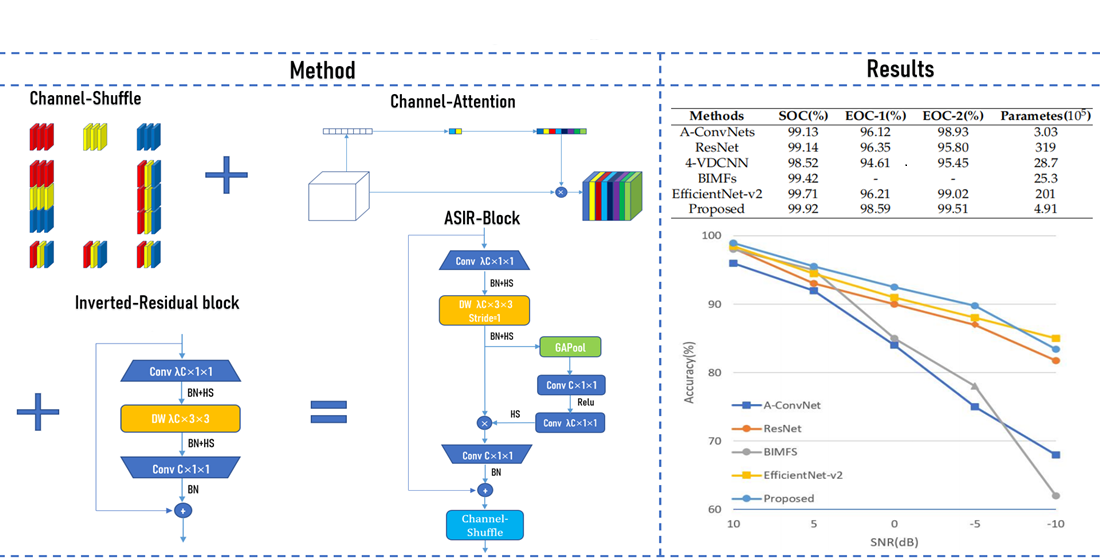
:Automatic target recognition (ATR) in synthetic aperture radar (SAR) images has been widely used in civilian and military fields. Traditional model-based methods and template matching methods do not work well under extended operating conditions (EOCs), such as depression angle variant, configuration variant, and noise corruption. To improve the recognition performance, methods based on convolutional neural networks (CNN) have been introduced to solve such problems and have shown outstanding performance. However, most of these methods rely on continuously increasing the width and depth of networks. This adds a large number of parameters and computational overhead, which is not conducive to deployment on edge devices. To solve these problems, a novel lightweight fully convolutional neural network based on Channel-Attention mechanism, Channel-Shuffle mechanism, and Inverted-Residual block, namely the ASIR-Net, is proposed in this paper. Specifically, we deploy Inverted-Residual blocks to extract features in high-dimensional space with fewer parameters and design a Channel-Attention mechanism to distribute different weights to different channels. Then, in order to increase the exchange of information between channels, we introduce the Channel-Shuffle mechanism into the Inverted-Residual block. Finally, to alleviate the matter of the scarcity of SAR images and strengthen the generalization performance of the network, four approaches of data augmentation are proposed. The effect and generalization performance of the proposed ASIR-Net have been proved by a lot of experiments under both SOC and EOCs on the MSTAR dataset. The experimental results indicate that ASIR-Net achieves higher recognition accuracy rates under both SOC and EOCs, which is better than the existing excellent ATR methods.

1. Introduction
SAR can work stably for a long time in harsh environments, and can provide high-quality images for earth observation, so that it has been used in the national defense construction and national economy widely, such as marine monitoring system, ship target recognition, mineral exploration, precision agriculture, etc. However, unlike commom optical images, the unipolar gray-scale SAR image has blurred edges and strong anisotropy owing to the imaging mechanism, speckle noise, and background clutter. These characteristics will affect the effective feature extraction and automatic target recognition (ATR) [1,2].
A great number of different methods are applied in the field of SAR ATR in the past few decades. Traditionally, those methods consist of model-based methods and template matching methods. The template matching method [3,4] is to generate a template database from training images according to manually designed rules, and then every test image is compared to the template database and match the most similar template. Although template matching is simple and popular [5], it requires manual template making and can easily cause overfitting problems. Different from the template matching method, the model-based method [6,7] mainly use computer-aided design models to describe the structural characteristics of the target as much as possible. This method has high recognition accuracy, but the modeling process is usually more complicated and requires higher professional knowledge of modelers.
Some machine learning methods also have been introduced into the field of SAR ATR. In the machine learning method, the main work is to construct a set of suitable feature extractors because it is usually task-specific. In Reference [8], support vector machine (SVM) was used to recognize SAR targets and outperformed some conventional methods. Sun and Liu [9] proposed adaptive boosting (AdaBoost) which use radial basis function (RBF) network to extract features. Carmine Clemente et al. [10] proposed a novel method from multiple spatially separated, multi-channel SAR data. It can use single-channel or multi-channel information, and the computational cost is low. In Reference [11], a method based on dictionary learning and joint dynamic sparse representation (DL-JDSR) is proposed for SAR ATR. Meiting Yu et al. [12] used a multi-scale components of the monogenic signal to extract the features of SAR images and proposed joint sparse and dense representation of monogenic signal (JMSDR). Jiahuan Zhang et al. [13] used the multi-grained cascade forest (gcForest) to construct a novel deep forest network for SAR ATR.
With the development of deep learning theory, it has been used in the fields of text, signal, image, and video, and has shown predominant performance because deep learning network has an end-to-end structure without complex manual preprocessing operations. This end-to-end structure can automatically learn the optimal discriminant information for a specific target from SAR images and extract some stable features for target recognition. Originally, E Zelnio and FD Garber [14] showed how to combine a CNN and an existing classifier to recognize testing targets that have not been seen before. Later, Jun Ding [15] used fully connected layers, convolutional layers, pooling layers, and a SoftMax classifier to build a classic convolutional neural network, and designed three approaches of data augmentation for SAR ATR. Carmine Clemente et al. [16] proposed a method based on Krawtchouk moments for SAR ATR, which can represent a detected extended target with few features. In Reference [17], an all-convolutional network (A-ConvNets) was proposed. The authors used convolutional layers to replace all fully connected layers for reducing network parameters and alleviating the problem of overfitting. Wagner et al. [18] proposed a network combining a CNN and a SVM, and additional training methods to incorporate prior knowledge. Maha Al Mufti et al. [19] used a pretrained AlexNet and a SVM as the classifier for SAR ATR. Furukawa et al. [20] utilized the deep residual network (ResNet) for SAR ATR. In order to efficiently extract target features with different azimuth angles, Pei et al. [21] designed a multi-view deep convolutional neural network (m-VDCNN). Shanshan Shang et al. [22] proposed bidimensional intrinsic mode functions (BIMFs) for SAR ATR, which is the combination of multi-mode representations extracted by bidimensional empirical mode decomposition (BEMD) and ResNet. Zhenpeng Feng et al. [23] proposed a Self-Matching class activation mapping (CAM) to improve the interpretability of SAR images.
Despite the fact that the aforementioned methods show excellent performance, they usually have a large number of computational overhead and parameters, so they are not conducive to deployment on edge devices. Furthermore, they rarely care about the generalization performance, such as the invariance under target translation, invariance under different depression angles, the tolerance of noise with different Signal-to-Noise Ratios (SNRs), and the tolerance of posture missing in training dataset. Therefore, this work proposes a novel lightweight CNN and four approaches of data augmentation for SAR ATR to achieve a higher accuracy under both SOC and EOCs, while reducing the number of parameters greatly. Primarily, this work strongly contributes based on the following:
- 1
- Design a novel lightweight fully convolutional neural network based on Channel-Attention mechanism, Channel-Shuffle mechanism, and Inverted-Residual block for SAR ATR. The utilization of Inverted-Residual block and Channel-attention mechanism is able to improve the representational power of the network. Channel-Shuffle mechanism can promote the exchange of information between channels. A series of comparative experiments on the MSTAR dataset [24] indicate that, compared to other excellent methods (e.g., A-ConvNets [17], ResNet [25], 4-VDCNN [21], BIMFs [22], and EfficientNet-v2 [26]), our ASIR-Net achieves higher recognition accuracy rates with a smaller number of parameters.
- 2
- Four approaches of data augmentation (shear, rotation, zoom, and flip) are proposed to alleviate the matter of the scarcity of SAR images and strengthen generalization ability of ASIR-Net. The experimental results under both SOC and EOCs show that the proposed ASIR-Net trained with the four data augmentation approaches achieves satisfactory performance.
The remainder of this paper is organized as follows: Section 2 explains the key technologies used to construct the proposed ASIR-Net, including Inverted-Residual block, depthwise convolution, batch normalization, Hard-Swish activation function, Channel-Attention mechanism, and Channel-Shuffle mechanism. Furthermore, the structure details, training of ASIR-Net, and dataset description are also given. Section 3 introduces the data augmentation approaches and a series of comparative experiments on MSTAR under both SOC and EOCs. Section 4 uses ablation studies to discusses the effect of the key technologies. Section 5 concludes this paper.
2. Materials and Methods
2.1. Inverted-Residual Block
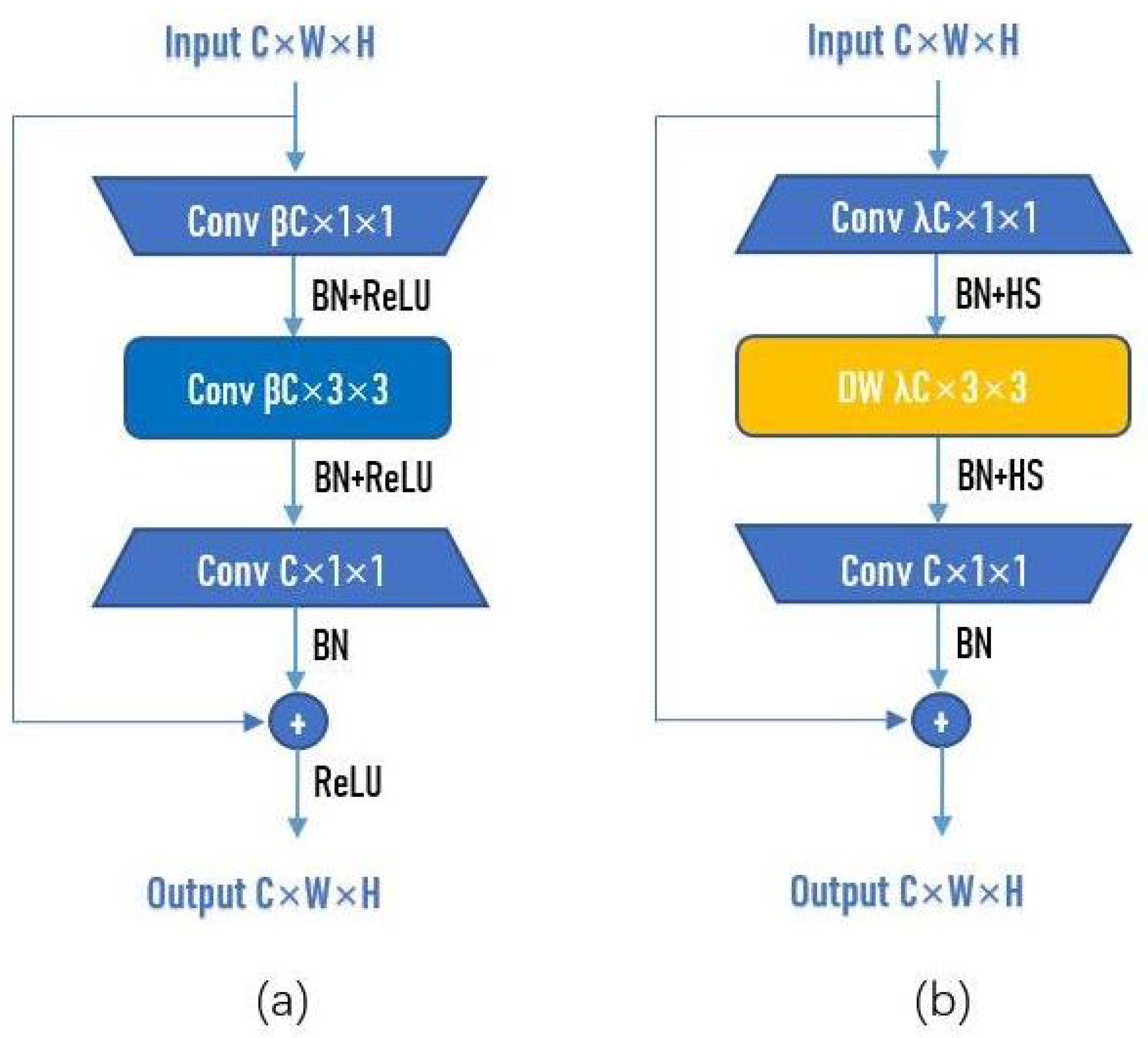
ResNet [25] was proposed in 2015 and won the championship in the classification task of the ImageNet competition. Because it is simple and practical, many methods are built on the basis of ResNet. It is widely used in recognition, detection, segmentation, and other fields. The Residual block is the main structure in ResNet, as shown in Figure 1a. Input C × W × H means that the number of channels of the input is C, and the width and height of channels of the input are W and H, respectively. Conv C × 1 × 1 means that the number of 1 × 1 convolutional kernels is C. After passing the first 1 × 1 convolutional layer, the width and height of the channel remain unchanged, and the number of channels becomes C. is a hyperparameter-scaling factor, usually set as = 0.25. The main purpose of the first 1 × 1 convolutional layer is to fusion the channels, thereby reducing the amount of calculation. After dimensionality reduction, parameters training and feature extraction can be performed more effectively and intuitively. The function of the middle 3 × 3 convolutional layer is to perform feature extraction in low-dimensional space. Set stride = 1 and padding = 1 to ensure that the width and height of the channel do not change. Finally, a 1 × 1 convolutional layer is used to restore the same dimensionality as the input.
However, a 1 × 1 convolutional layer is first used to increase the dimensionality of the input in the Inverted-Residual block. After passing the first 1 × 1 convolutional layer, the width and height of the channel remain unchanged, and the number of channels becomes C. is a hyperparameter-scaling factor, and set = 4 or 6 in this paper. Then, use depthwise convolution (DW) for feature extraction. Finally, for more effective use of information of different channels at the same spatial position, a 1 × 1 convolutional layer is utilized to fuse channels and restore the same dimensionality as the input.
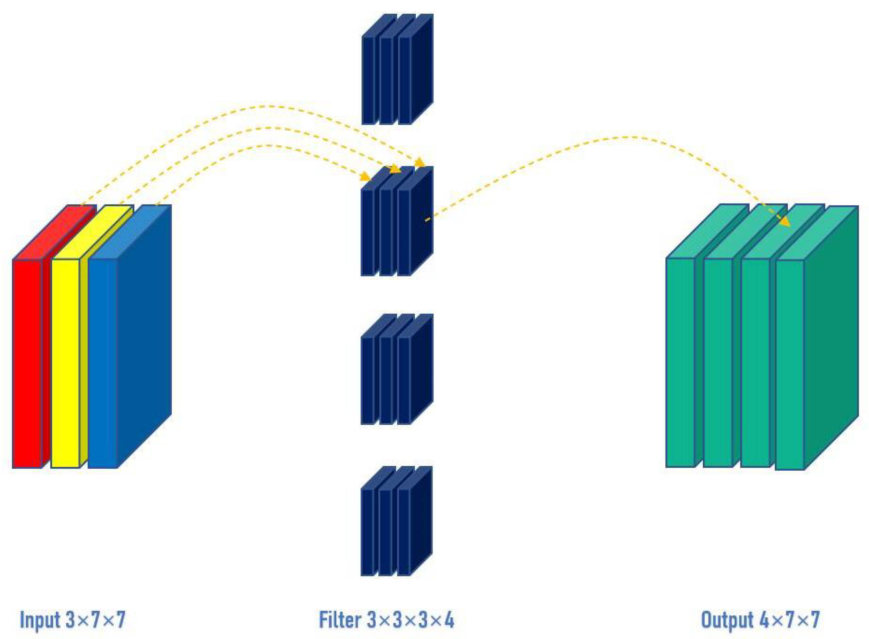
For conventional convolution, input a three-channel, and 7 × 7 pixel image (shape: 3 × 7 × 7), after passing the 3 × 3 convolutional layer (assuming the number of convolutional kernels is 4, the shape of the convolutional kernel is 3 × 3 × 3 × 4), and, finally, 4 channels are output. If the same padding is set, the size of the output is the same as the input (7 × 7); if not, the size of the output becomes 5 × 5, as shown in Figure 2.
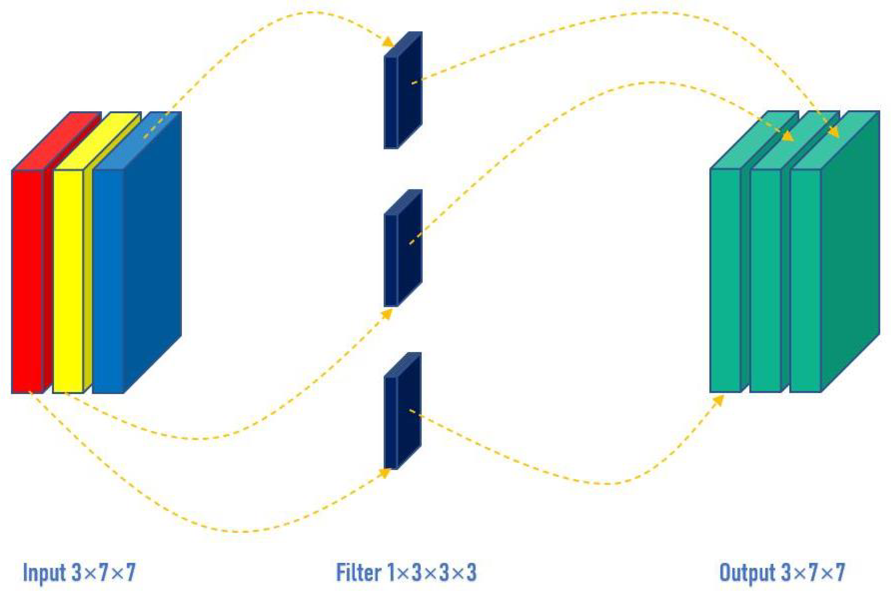
However, for depthwise convolution (DW), one channel is convolved by one convolutional kernel, and one convolutional kernel is only responsible for one channel. For the aforementioned conventional convolution, each convolutional kernel is to operate all channels of the input image at the same time. Similarly, input a three-channel, and 7 × 7 pixel image (shape: 3 × 7 × 7), DW is completely convolved in two-dimensional space. The number of channels of the input and the number of convolutional kernels are the same, and there is a one-to-one correspondence between channels and convolutional kernels. So, a three-channel image generates three channels after passing the DW layer. If the same padding is set, the size of the output is the same as the input (7 × 7); if not, the size of the output becomes 5 × 5, as shown in Figure 3. By keeping the number of trainable weight parameters required at a low level, DW can reduce network complexity while maintaining high recognition accuracy. DW can separate the channel and the convolution area, and connect the input and output channels one-to-one through the convolution operation.
In both the Residual block and Inverted-Residual block, when the shape of the ouput is the same as that of the input, a shortcut connection can be used. The formula of the shortcut connection can be summarized as:
where represents the feature extraction process, u represents the input, and represents the output. Many neural network experiments before the emergence of ResNet show that an appropriate increase in the depth of the network will strengthen its performance, but, after a certain level, the opposite effect may be achieved. Due to the divergence of the gradient, the network may be degraded. However, the shortcut connection in Residual block cleverly solves this problem.
A batch normalization (BN) operation is required between each convolutional layer and activation function. Before the nonlinear transformation, the input value of the deep convolutional neural network is gradually moved or changed as the network deepens, which results in the gradient disappearance of the deeper neural layer during the back propagation process. This is the root cause of the slower and slower training speed of deep convolutional neural networks. BN can avoid the gradient explosion and gradient disappear by modifying the distribution of the input data, thereby pulling most of the input data into the linear part of the activation function. Suppose a batch of input data is , the process of BN can be divided into 3 steps, as follows. Step 1: the average and variance of the batch D can be obtained by:
where is the variance of the batch D, and is the average of the batch D. Step 2: the batch D is normalized by and to get the 0–1 distribution:
where is a very small positive number to prevent the divisor from becoming 0. Step 3: scale and translate the normalized batch D by:
where and are scale factor and translation factor, respectively [27]. represents the operation of BN.
In Residual block, ReLU which has much less computation than sigmoid [28] is used as the activation function. It can improve the convergence speed and alleviate the problem of gradient disappearance. The formula of the ReLU is presented as:
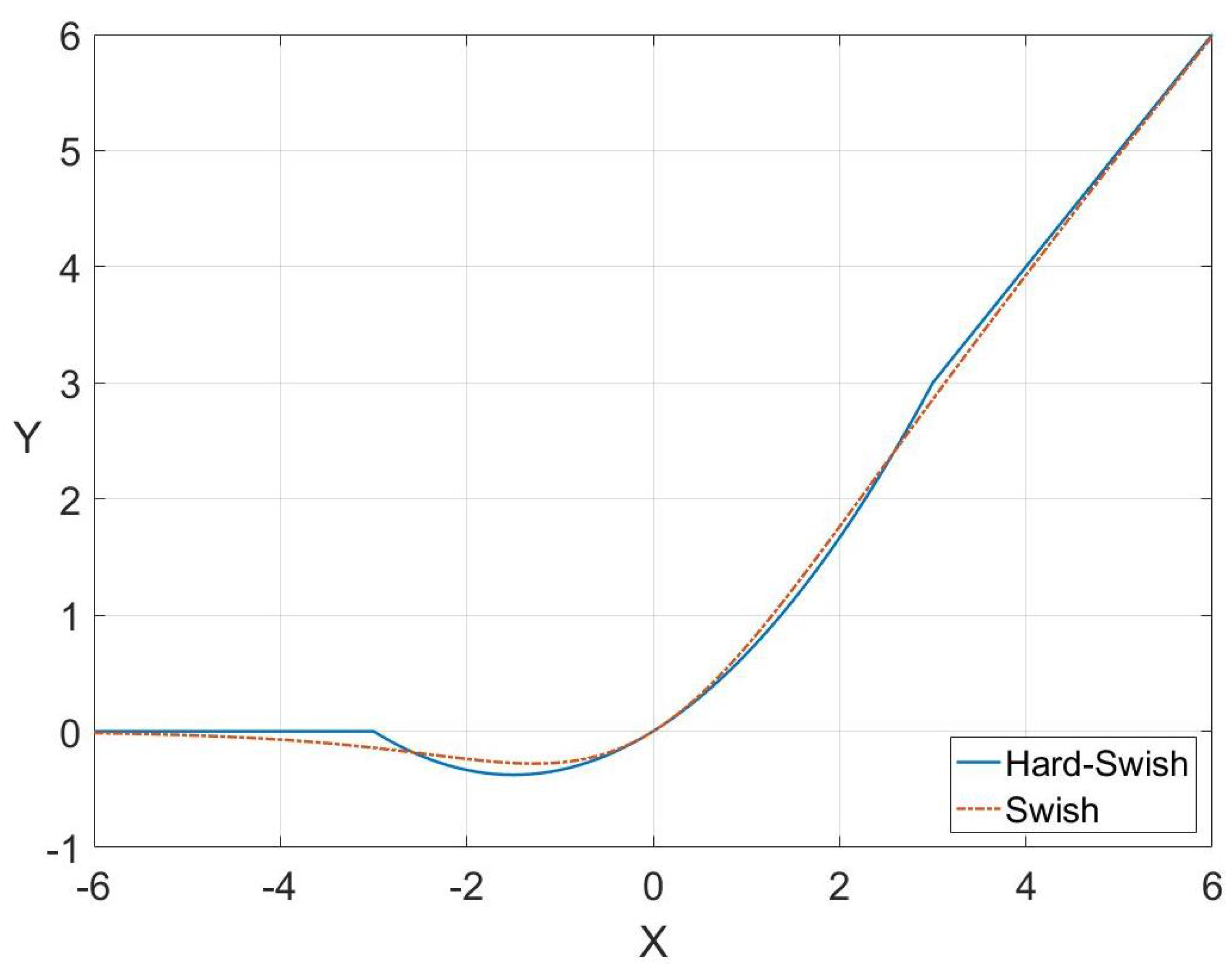
In the Inverted-residual block, Hard-Swish (HS) [29] is used as the activation function. In deep neural networks, the Swish activation function has been shown to perform better than ReLU [30]. The function has the good characteristics of lower bound, no upper bound, non-monotonic, and smooth, which is presented as:
where is a trainable parameter or constant. But, compared to ReLU, its calculation is more complicated because of the sigmoid function. Therefore, the sigmoid function is replaced with the ReLU6 function so as to reduce the amount of calculation, and the Hard-Swish (HS) is obtained. Hard-Swish is presented as:
The graphics of Swish and Hard-Swish are similar, but the amount of calculation of Hard-Swish is much smaller in the back propagation process. The comparison of Swish and Hard-Swish is shown in Figure 4.
2.2. Channel-Attention Mechanism
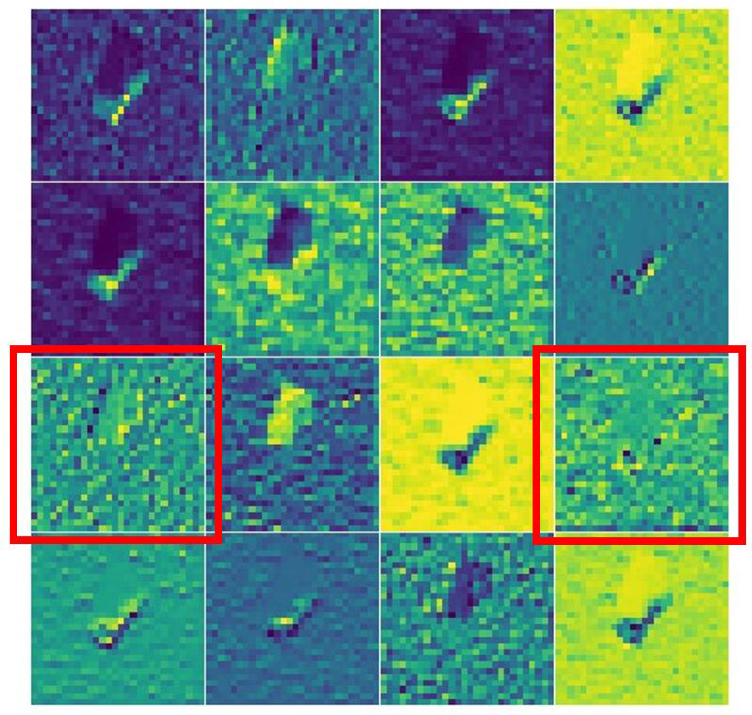
A traditional CNN includes feature extraction modules and a classifier. Each channel of the same layer has the same status to the next layer in a traditional feature extract module. But this assumption is often proven wrong in practice [31]. In our previous experiments, we used multiple Inverted-Residual block in series to extract feature maps, and SoftMax as a classifier. Figure 5 displays the 16 feature maps which are extracted by the second DW layer. It is obvious that some feature maps only extract background clutter and contain less target structure information, such as the first and fourth feature maps in the third row.
In the aforementioned traditional CNN, all channels which contain different information in the same convolutional layer pass through the next convolutional layer equally. Therefore, their contribution to recognition is equal, and this equal mechanism interferes with the use of important channels which contain more useful information. So, we try to introduce the Channel-Attention mechanism. Channel-Attention mechanism can allocate different weights to channels of different importance levels in the same convolutional layer to strengthen channels that contain important information and stifle channels that contain useless information. Figure 6 illustrates the principle of the Channel-Attention module.
C × W × H means that the width and height of the input U are W and H, respectively, and the number of channels of the input U is C. GAPool represents global average pooling, which is presented as:
where represents the kth channel of U. After passing GAPool, the dimensionality of U becomes C × 1 × 1. Then, two 1 × 1 convolutional layers are used instead of the fully connected layer of common attention modules, which can effectively reduce the parameters of the attention module. After passing the two 1 × 1 convolutional layers, U becomes an automatically updated weight vector, representing the importance of different channels. The activation functions of the first convolutional layer and the second convolutional layer are ReLU and Hard-Swish, respectively. Finally, the kth channel generated by the Channel-Attention module is expressed as:
where represents the weight of , and represents the product of them.
2.3. Channel-Shuffle Mechanism
Although DW can extract features in high-dimensional space with fewer parameters, DW will hinder the exchange of information between different channels. The 1 × 1 convolutional layer can alleviate this shortcoming, but it is not enough. So, we try to introduce the Channel-Shuffle mechanism to the Inverted-Residual block. The Channel-Shuffle mechanism can make the output of a channel not only related to its corresponding input, which can promote the exchange of information between channels and describe more detailed features.
Channel-Shuffle mechanism was first proposed in ShuffleNet [32]. In ShuffleNet, the author uses Channel-Shuffle mechanism to overcome the problem of low information flow rate between channels in group convolution. The specific operation steps of Channel-Shuffle mechanism are shown in Figure 7. Step 1: divide the input C channels into g groups equally, each group contains n channels (C = 9, g = 3, n = 3 in Figure 7); Step 2: reshape the dimensionality of input from [N, g × n, W, H ] to [N, g, n, W, H]; Step 3: transpose the g and n; Step 4: restore the dimensionality of the data to [N, n × g, W, H]. After passing Channel-Shuffle module, each group of channels finally obtained contains the channels of other groups before the Channel-Shuffle module.
2.4. Network Architecture of ASIR-Net
After adding Channel-Attention mechanism and Channel-Shuffle mechanism to the Inverted-Residual block and using the 1 × 1 convolutional layers instead of the fully connected layers, we get a fully convolutional network, namely ASIR-Net.
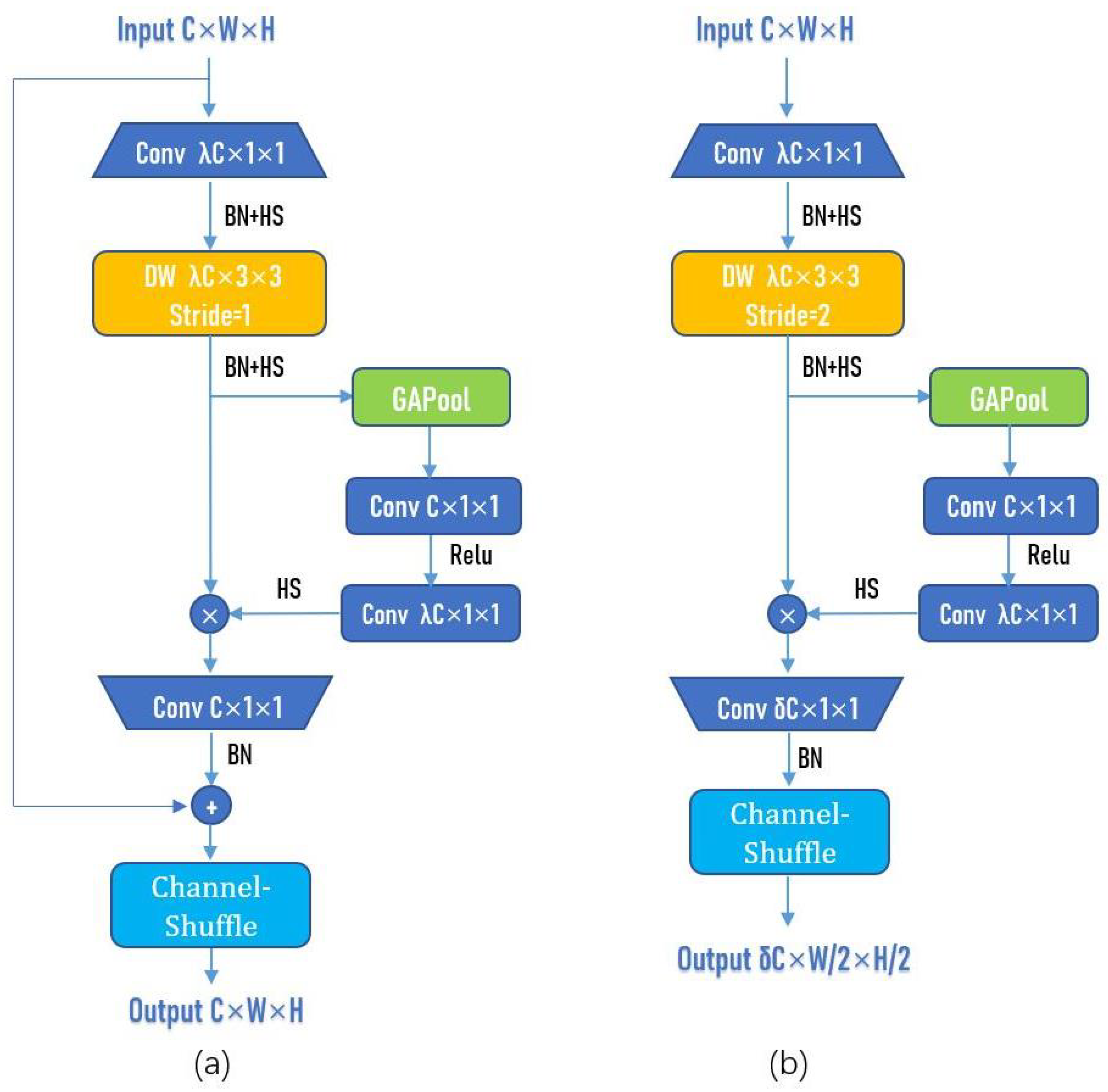
Next, we will discuss the features and overall structure of the proposed ASIR-Net. There are two blocks in ASIR-Net, namely ASIR-Block (stride = 1) and ASIR-Block (stride = 2), as shown in Figure 8a,b.
In the ASIR-Block (stride = 1), the stride of DW is set as 1, the pooling is set as the same, and the number of convolutional kernels in the last 1 × 1 convolutional layer and the number of channels of the input are the same, so as to ensure that the shape of the output is the same as that of the input, and a shortcut connection can be used. The ASIR-Block (stride = 1) is used in the second half of the ASIR-Net to ensure the training effect and accelerate the training speed. In the ASIR-Block (stride = 2), the stride of DW is set as 2, the pooling is set as the same, and the number of convolutional kernels in the last 1 × 1 convolutional layer is set as C; is a hyperparameter, generally set as 2 or 3. The width and height of the output have become half of the input, and the number of channels of the output has become times that of the input. The ASIR-Block (stride = 2) is used in the first half of the network to compress the width and height of the channel and increase the number of channels.
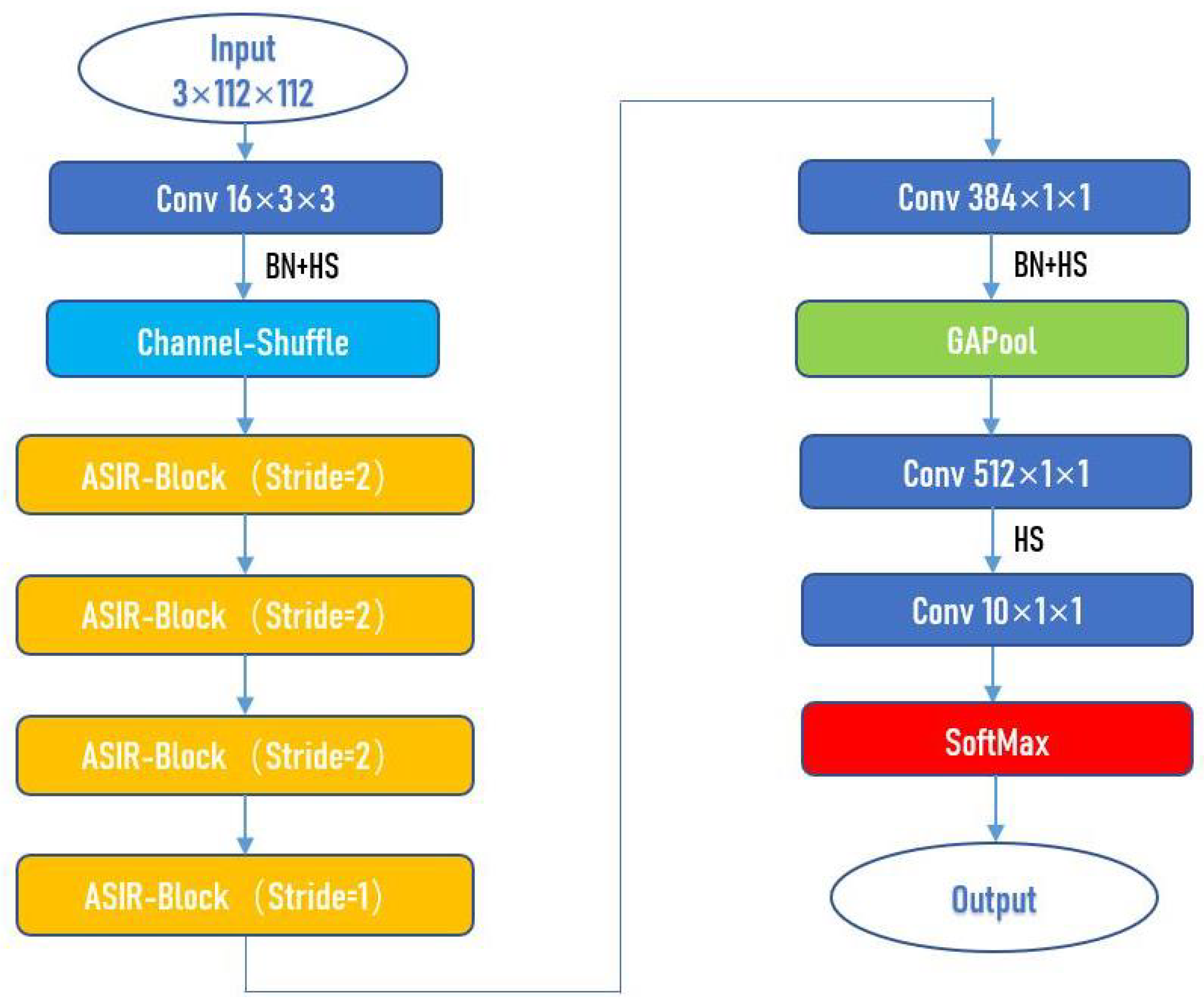
With referencing to the network structure and hyperparameters of ShuffleNet [32] and EfficientNet-v2 [26] and doing a lot of experiments based on the structure and hyperparameters of these networks, we finally determined the structure and hyperparameters of our network. See Table 1 and Figure 9 for the complete specifications of ASIR-Net, where Out denotes the number of output channels, BN denotes whether to perform Batch-Normalization after the convolutional layer, NL denotes the type of nonlinear activation function used, and s denotes stride.
2.5. Training of ASIR-Net
We use SoftMax as the classifier. Softmax can map output values to the values in the interval (0,1), and the sum of the transformed values is 1, so we can understand the transformed values as probabilities. Suppose the vector which inputs to SoftMax is , the formula of SoftMax is expressed as:
where is the power of e, is the one-hot probability vector corresponding to the target types, and C represents the number of target types. After passing the SoftMax, we can obtain the probability of each element corresponding to various targets from the output vector.
We use Cross-entropy as the loss function. Suppose a batch of samples in dataset is , where is the true label of . The Cross-entropy can be presented as:
Adam [33] is used to update the trainable parameters of the proposed ASIR-Net. For the weight , we can update it in this way:
where t denotes number of updates, is the correction of , is the correction of , and the formula of and can be presented as:
where and are constants and control exponential decay. is the exponential moving average of the gradient, which is obtained by the first moment of the gradient. is the square gradient, which is obtained by the second moment of the gradient. The updates of and can be expressed as:
where is the first derivative. The aforementioned parameters are set as: , = 0.9, = 0.999, = 0.001.
2.6. Dataset Description
Unlike the rapid development of optical image recognition research, in the field of SAR ATR, it is very difficult to get sufficient publicly available datasets because of the difficulty of target detection means. Among them, the MSTAR publicly available in the United States is one of the few datasets that can identify ground vehicle targets. MSTAR was launched by the Defense Advanced Research Projects Agency (DARPA) in the mid-1990s [34]. High resolution focused SAR is used to collect SAR images of various military vehicles in the former Soviet Union. MSTAR plans to conduct SAR field tests on ground targets, including target occlusion, camouflage, configuration changes, and other scalability conditions, to form a relatively comprehensive and systematic field test database. The international research on SAR ATR is basically based on this dataset, up to now.
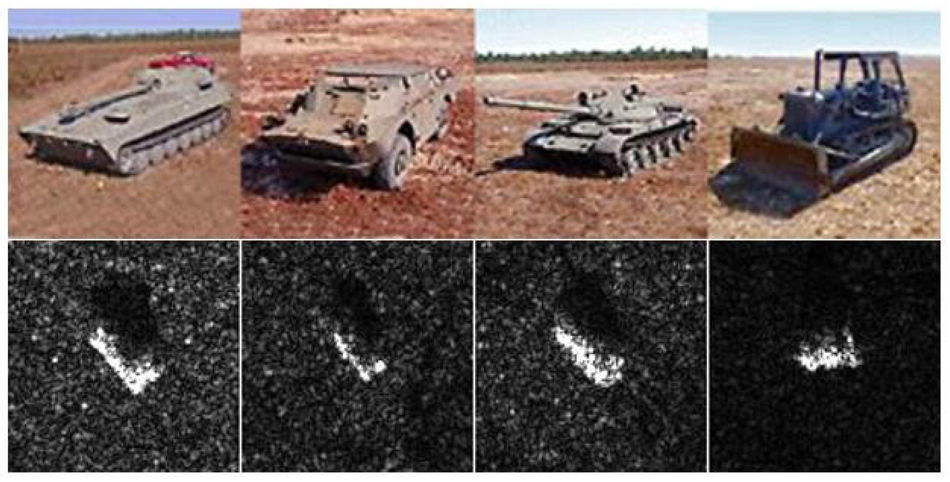
The MSTAR dataset consists of ten types of targets: ZSU234, ZIL131, T72, T62, D7, BTR70, BTR60, BRDM2, BMP2, and 2S1. The x-band imaging radar works in HH polarization mode and obtains a serious of images with a size of 158 × 158 pixels and a resolution of 0.3 × 0.3 m [35]. Figure 10 depicts optical images and corresponding SAR images of targets at a similar angle.
There are two categorise of collection conditions in MSTAR dataset: Standard Operating Condition (SOC) and Extended Operating Conditions (EOCs). These SAR images are generated based on a variety of acquisition conditions, such as changing the imaging depression angle, target posture, or target serial number. SOC means that the sequence number and target configuration of training dataset are the same as that of testing dataset, but the depression angles are different. EOCs consist of three experiments: depression angle variant, configuration variant, and noise corruption. Unlike some papers which only verify the performance of the network under SOC [19,36], to evaluate the generalization performance of the proposed ASIR-Net, this paper also measure the recognition accuracy rates of the proposed ASIR-Net under EOCs.
3. Experiments and Results
3.1. Data Augmentation and Network Setup
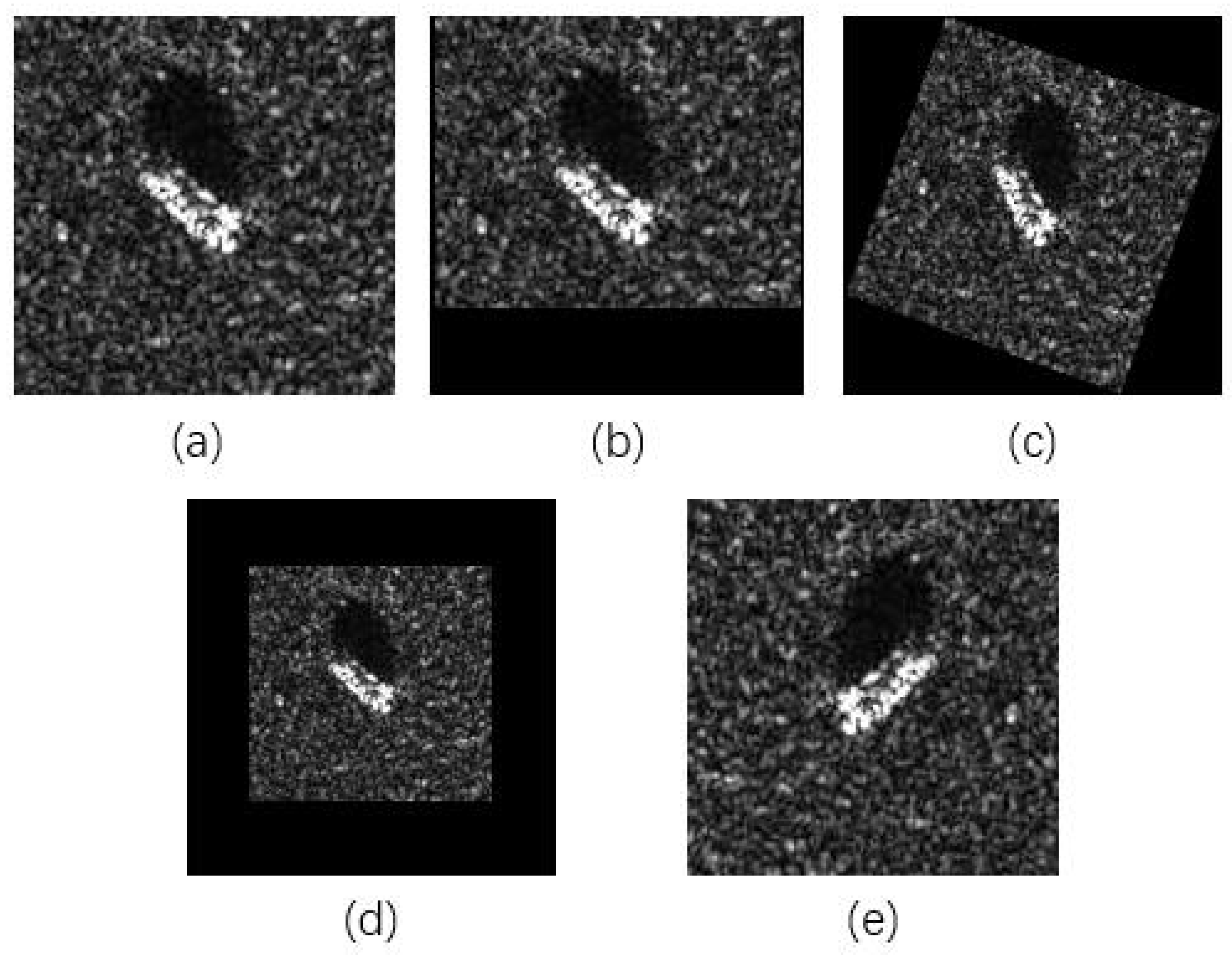
In general, the larger the number of samples, the better the training effect of the network. However, due to the scarcity of SAR images, we must explore a variety of methods to augment the dataset. Next, we will introduce four approaches of data augmentation. (a) random shear: cut out part of the target in the image, which helps to learn part of structural features of the target; (b) rotation: image rotation technology allows the network to learn the characteristics of rotation invariance, which can alleviate the problem of less posture in the sample; (c) zoom: zooming in or zooming out the image helps to learn the target features under different resolutions; (d) flip: similar to the rotation, the network can learn more about postures of the target. In the experiments below, shear range is set to 0.2, zoom range is set to 0.2, rotation range is set to 10°, and horizontal flip is set to True. The effect of four approaches of data augmentation is shown in Figure 11.
The width and height of the input SAR images are both 112, and the number of channels of the input SAR images is 1. But we set the number of input image channels of ASIR-Net to 3, so that ASIR-Net can be applied to target recognition in three-channel RGB images. Such a setting can expand the application fields of ASIR-Net. When a single-channel SAR image is input to ASIR-Net, the ’Input’ function in our network will convert it into a three-channel image, and the three channels are the same. But after passing the first convolutional layer, all channels become different, as shown in Figure 5. Hyperparameters in the proposed ASIR-Net are shown in Table 1. The weights are initialized using the He-initialization method [37] which can ensure that information can flow effectively in the process of forward and backward propagation, so that the variances of the input signals of different layers are roughly equal. The original learning rate is set as 0.0005 and gradually decays to 0.0001.
The proposed ASIR-Net is built using the framework of TensorFlow2.4 and implemented on NVIDIA GTX2060 GPU.
3.2. Recognition Results under SOC
In the SOC experiment, classification task of ten target classes was used to measure the recognition accuracy rate of the proposed ASIR-Net. As shown in Table 2, the training dataset is collected under a 17° depression angle, and the testing dataset is collected under a 15° depression angle. There are 2747 SAR images in the training dataset and 2425 SAR images in the testing dataset.
The recognition result of the proposed ASIR-Net is shown in Table 3 which is a confusion matrix of the recognition task of ten targets. In the field of deep learning, the confusion matrix, which is also called the error matrix or possibility table, is a standard format for recognition accuracy evaluation. It is able to visualize the performance of supervised learning algorithms. Every column represents the actual category, every row represents the predicted category, and the number on the diagonal is the number of correct predictions for each category.
The recognition accuracy rates of 2S1 and T72 are 99.64% and 99.49%, respectively, and that of the others is 100%. The overall recognition accuracy rate of the entire dataset has reached an astonishing 99.92%. The experimental result shows that some stable features that can effectively recognize different targets are extracted through a serious of ASIR-Blocks. This is the dominant cause why the proposed ASIR-Net can achieve a such good result in the SOC experiment.
3.3. Recognition Results under EOC
Target recognition under different combat conditions is more complicated in the real battlefield situation, so it is very necessary to measure the generalization ability of the proposed ASIR-Net under EOCs.
EOC-1 (Large Depression Variant): Large changes in depression angle will make a great difference in the corresponding SAR images because the SAR image is sensitive to the imaging depression angle. Referring to the experiments in literature [38,39], select ZSU234, T72, BRDM2, and 2S1 as the training dataset and testing dataset, as shown in Table 4. The depression angle in the testing dataset is 30°, while the depression angle in the training dataset is 17°.
Table 5 shows the recognition result of ASIR-Net in the EOC-1 experiment. The total recognition accuracy rate is 97.83% and the recognition accuracy rates of T72, ZSU-234, BRDM-2, and 2S1 are 100%, 97.92%, 97.91%, and 95.49%, respectively. A small part of 2S1 was misidentified as BRDM2, which may be due to the fact that 2S1 and BRDM2 have a high degree of similarity at 30° depression angle. The experimental result indicates that the proposed ASIR-Net has good performance under different depression angles.
EOC-2 (Configuration Variant): The configurations of targets in the training dataset and testing dataset are different, such as equipped with different reactive armor or auxiliary tanks. There are 4 types of targets in the training dataset (T-72, BTR-70, BRDM-2, and BMP-2), but only the T-72 target with five configuration variants is in the testing dataset, as shown in Table 6.
Table 7 shows the recognition accuracy rate of the proposed ASIR-Net in the EOC-2 experiment and the total recognition accuracy rate is 99.51%. It is obvious that the proposed ASIR-Net can accurately identify the targets with different configurations.
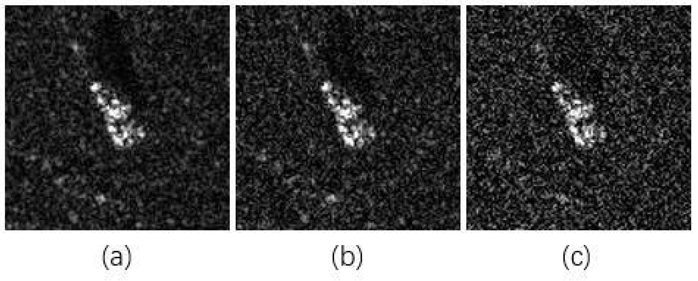
EOC-3 (Noise Corruption): SAR image will be mixed with noise generated by the radar system and the environment, which will affect the accuracy of target classification. Therefore, to evaluate the ability of the proposed ASIR-Net to identify targets under noise interference with different SNRs, the complex additive white Gaussian noise (AWGN) has been added to the SAR images in the SOC dataset [40]. The 2S1 images damaged by noise with different SNRs are shown in Figure 12a–c.
Table 8 shows the recognition accuracy rates of the proposed ASIR-Net in the EOC-3 experiment. When the SNR is −10dB, the recognition accuracy rate is only 83.4% because the target characteristics are blurred by the noise, especially, at low SNRs.
3.4. Methods Comparison
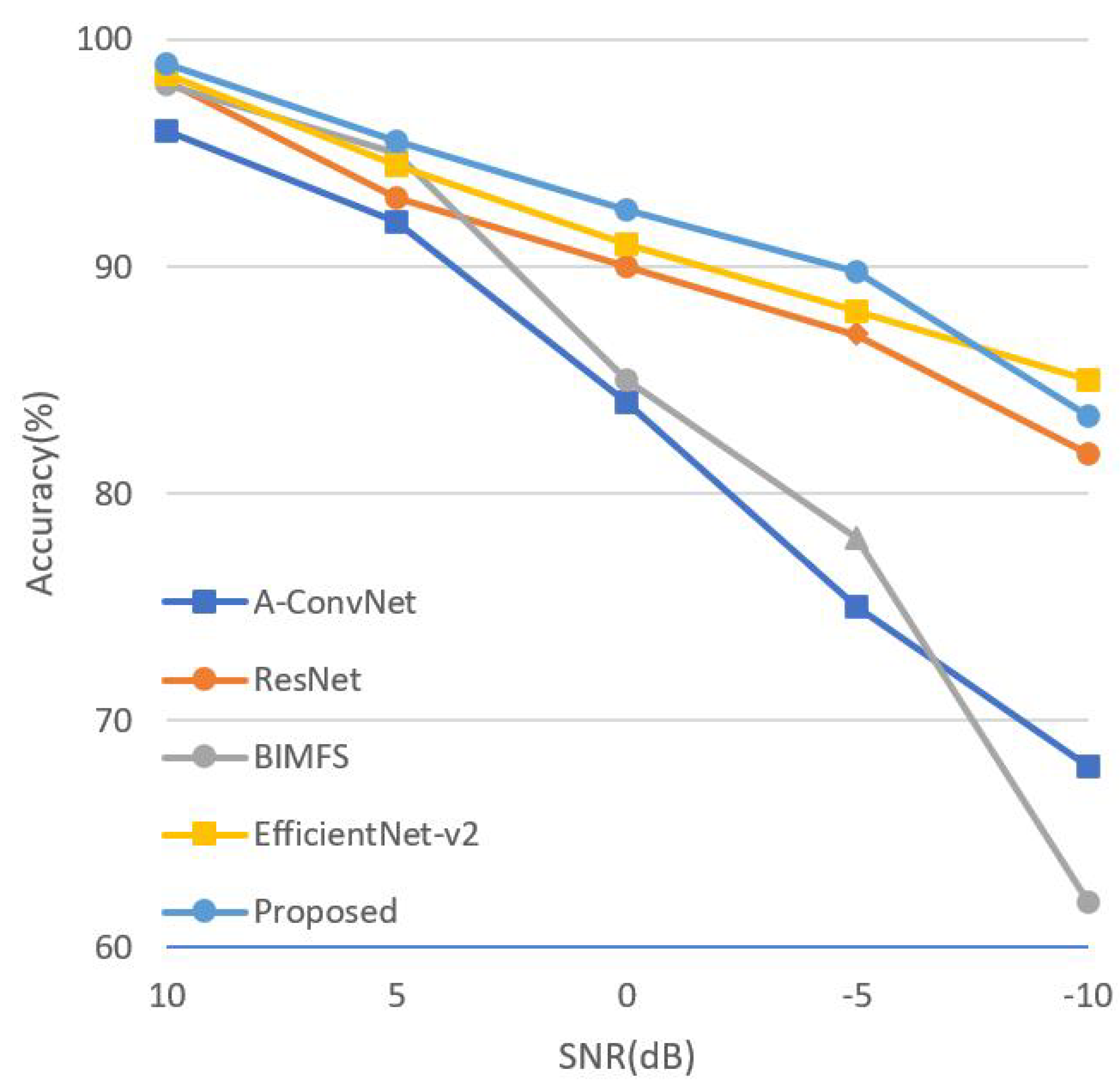
In this section, the proposed ASIR-Net is compared with five other SAR ATR methods, as shown in Table 9 and Figure 13. These methods are A-ConvNets [17], ResNet [25], 4-VDCNN [21], BIMFs [22], and EfficientNet-v2 [26]. Table 9 and Figure 13 indicates that the proposed ASIR-Net is superior to other methods in recognition accuracy rates under both SOC and EOCs, and requires much smaller number of parameters than the other four SAR ATR methods except A-ConvNets. In the SOC experiment, the recognition accuracy rates of all methods are above 98%, but, in the EOCs experiment, the recognition accuracy rates of these methods vary dramatically. ASIR-Net has slightly more parameters than A-ConvNets, but the performance of ASIR-Net is much better than A-ConvNets, especially in the EOC-3 experiment. The performance of ASIR-Net is better than EfficientNet-v2 a little, but the number of parameters of ASIR-Net is only about 1/40 of that of EfficientNet-v2.
From the aforementioned experimental results, it is obvious that the proposed lightweight ASIR-Net has excellent recognition capabilities under both SOC and EOCs, verifying the superiority of the proposed network and approaches of data augmentation.
4. Discussion
In this section, ablation studies were uesd to discuss the effect of the fully convolutional (FC) neural network, Channel-Attention (CA) mechanism, Channel-Shuffle (CS) mechanism, and Inverted-Residual (IR) block. Referring to the ablation studies in literature [41,42], we design four variants of our ASIR-Net as follows for comparison:
- 1
- CNN: CNN is a traditional convolutional neural network with the same number of network layers as the proposed ASIR-Net. It consists of convolutional layers, BN layers, ReLU activation functions, fully connected layers, and a SoftMax classifier.
- 2
- FCNN: By replacing all the fully connected layers of CNN with 1 × 1 convolutional layers, we get FCNN. We can evaluate the effect of replacing the fully connected layers with 1 × 1 convolutional layers by comparing the performance and parameters of CNN and FCNN.
- 3
- IR-Net: The traditional convolutional layers in FCNN are replaced by the Inverted-Residual blocks, and IR-Net is obtained. The effect of the Inverted-Residual blocks can be demonstrated by comparing the performance and parameters of FCNN and IR-Net.
- 4
- AIR-Net: AIR-Net is obtained by adding the Channel-Attention mechanism into IR-Net. The effect of the Channel-Attention mechanism can be demonstrated by comparing the performance of IR-Net and AIR-Net, and the effect of the Channel-Shuffle mechanism can be proved by comparing the performance of AIR-Net and ASIR-Net.
The detailed configurations, experimental results, and number of parameters of the different variants are shown in Table 10.
FCNN: It can be seen from the first and second rows of Table 10 that the performance can be improved, and the number of parameters can be greatly reduced, after the fully connected layers are replaced with the 1 × 1 convolutional layers because the fully connected layers have a large number of parameters, which is easy to cause over-fitting problems.
IR-block: As shown in the second and third rows of Table 10, the performance of FCNN and IR-Net is similar, but the number of parameters of IR-Net is less. It proves that traditional convolution and DW in Inverted-Residual block can both effectively extract some stable features for target recognition, but DW has fewer parameters.
Channel-Attention-mechanism: Compared with IR-Net, the performance of AIR-Net has been significantly improved and only a few parameters have been added, as shown in the third and fourth rows of Table 10, which fully shows the effectiveness of the designed Channel-Attention mechanism.
Channel-Shuffle-mechanism: As shown in the fourth and fifth rows of Table 10, AIR-Net and ASIR-Net have the same number of parameters because there is no trainable parameter in the Channel-Shuffle mechanism. Furthermore, ASIR-Net has superior performance, especially in the EOCs experiments, which demonstrates that the Channel-Shuffle mechanism can indeed promote the exchange of information between channels and describe more detailed features.
5. Conclusions
Deep learning theory has promoted the development of SAR ATR, but it is still challenging to train deep convolutional neural networks without enough original SAR images. In this paper, four approaches of data augmentation and a lightweight fully convolutional neural network based on Channel-Attention mechanism, Channel-Shuffle mechanism, and Inverted-Residual block are presented and applied to the SAR ATR problem. A series of experiments are performed to evaluate the proposed ASIR-Net on the MSTAR dataset, from which the following conclusions can be obtained:
- 1
- The lightweight ASIR-Net achieves higher recognition accuracy and has fewer parameters compared with other excellent methods.
- 2
- The recognition performance improves remarkably when introducing the Channel-Attention mechanism into networks because it can improve the representational power of networks.
- 3
- The depthwise convolution and Channel-Shuffle mechanism need to be used together. Although the depthwise convolution can extract features with fewer parameters, it will hinder information exchange between channels. The Channel-Shuffle mechanism can make up for this shortcoming.
- 4
- Using 1 × 1 convolutional layers instead of fully connected layers at the end of networks can greatly reduce the number of parameters and alleviate over-fitting problems.
Despite achieving good performance, the method in this paper still has a relatively low recognition accuracy when SAR images have a low signal-to-noise ratio. In the future, we will try to introduce a lightweight denoising mechanism into our network. More importantly, we will focus on introducing our ASIR-Net as the backbone into other target detection methods to achieve a wide range of applications in other fields, such as the ship target detection and instance segmentation for high-resolution SAR images.
Author Contributions
Conceptualization, J.Y. (Jimin Yu) and G.Z.; Data curation, G.Z.; Formal analysis, J.Y. (Jiajun Yin); Funding acquisition, S.Z.; Investigation, G.Z.; Methodology, J.Y. (Jimin Yu) and S.Z.; Project administration, J.Y. (Jimin Yu); Resources, J.Y. (Jimin Yu) and S.Z.; Software, G.Z. and J.Y. (Jiajun Yin); Supervision, J.Y. (Jimin Yu); Validation, G.Z., S.Z. and J.Y. (Jiajun Yin); Visualization, G.Z.; Writing—original draft, G.Z.; Writing—review & editing, J.Y. (Jimin Yu) and S.Z. All authors have read and agreed to the published version of the manuscript.
Funding
This work was supported by Chongqing Key Lab of Computer Network and Communication Technology (CY-CNCL-2017-02), the Science and Technology Research Project of Higher Education of Hebei Province (Grant No. QN2019069), NSFC (Grant Nos. 61701060 and 61801067), and Guangxi Colleges and Universities Key Laboratory of Intelligent Processing of Computer Images and Graphics Project (No.GIIP1806).
Institutional Review Board Statement
Not applicable.
Informed Consent Statement
Not applicable.
Data Availability Statement
The MSTAR dataset used to support the findings of this study is available online at http://www.sdms.afrl.af.mil/datasets/mstar/, accessed on 14 July 2021.
Conflicts of Interest
The authors declare no conflict of interest.
References
- Tait, P. Introduction to Radar Target Recognition; IET: London, UK, 2005; Volume 18. [Google Scholar]
- Novak, L.M.; Benitz, G.R.; Owirka, G.J.; Bessette, L.A. ATR performance using enhanced resolution SAR. Algorithms Synth. Aperture Radar Imag. III 1996, 2757, 332–337. [Google Scholar]
- Novak, L.M.; Owirka, G.J.; Brower, W.S.; Weaver, A.L. The automatic target-recognition system in SAIP. Linc. Lab. J. 1997, 10, 2. [Google Scholar]
- Owirka, G.J.; Verbout, S.M.; Novak, L.M. Template-based SAR ATR performance using different image enhancement techniques. Algorithms Synth. Aperture Radar Imag. VI 1999, 3721, 302–319. [Google Scholar]
- El-Darymli, K.; Gill, E.W.; Mcguire, P.; Power, D.; Moloney, C. Automatic Target Recognition in Synthetic Aperture Radar Imagery: A State-of-the-Art Review. IEEE Access 2016, 4, 6014–6058. [Google Scholar] [CrossRef] [Green Version]
- Ikeuchi, K.; Wheeler, M.D.; Yamazaki, T.; Shakunaga, T. Model-based SAR ATR system. Algorithms Synth. Aperture Radar Imag. III 1996, 2757, 376–387. [Google Scholar]
- Chiang, H.C.; Moses, R.L.; Potter, L.C. Model-based classification of radar images. IEEE Trans. Inf. Theory 2000, 46, 1842–1854. [Google Scholar] [CrossRef]
- Zhao, Q.; Principe, J.C. Support vector machines for SAR automatic target recognition. IEEE Trans. Aerosp. Electron. Syst. 2001, 37, 643–654. [Google Scholar] [CrossRef] [Green Version]
- Sun, Y.; Liu, Z.; Todorovic, S.; Li, J. Adaptive boosting for SAR automatic target recognition. IEEE Trans. Aerosp. Electron. Syst. 2007, 43, 112–125. [Google Scholar] [CrossRef]
- Clemente, C.; Pallotta, L.; Proudler, I.; De Maio, A.; Soraghan, J.J.; Farina, A. Pseudo-Zernike-based multi-pass automatic target recognition from multi-channel synthetic aperture radar. IET Radar Sonar Navig. 2015, 9, 457–466. [Google Scholar] [CrossRef] [Green Version]
- Sun, Y.; Du, L.; Wang, Y.; Wang, Y.; Hu, J. SAR automatic target recognition based on dictionary learning and joint dynamic sparse representation. IEEE Geosci. Remote Sens. Lett. 2016, 13, 1777–1781. [Google Scholar] [CrossRef]
- Yu, M.; Quan, S.; Kuang, G.; Ni, S. SAR target recognition via joint sparse and dense representation of monogenic signal. Remote Sens. 2019, 11, 2676. [Google Scholar] [CrossRef] [Green Version]
- Zhang, J.; Song, H.; Zhou, B. SAR target classification based on deep forest model. Remote Sens. 2020, 12, 128. [Google Scholar] [CrossRef] [Green Version]
- Zelnio, E.; Garber, F.D.; Morgan, D. Deep convolutional neural networks for ATR from SAR imagery. In Proceedings of the Algorithms for Synthetic Aperture Radar Imagery XXII, Baltimore, MD, USA, 20–24 April 2015; p. 94750F. [Google Scholar] [CrossRef]
- Ding, J.; Chen, B.; Liu, H.; Huang, M. Convolutional Neural Network With Data Augmentation for SAR Target Recognition. IEEE Geosci. Remote Sens. Lett. 2016, 13, 364–368. [Google Scholar] [CrossRef]
- Clemente, C.; Pallotta, L.; Gaglione, D.; De Maio, A.; Soraghan, J.J. Automatic Target Recognition of Military Vehicles With Krawtchouk Moments. IEEE Trans. Aerosp. Electron. Syst. 2017, 53, 493–500. [Google Scholar] [CrossRef] [Green Version]
- Chen, S.; Wang, H.; Xu, F.; Jin, Y. Target Classification Using the Deep Convolutional Networks for SAR Images. IEEE Trans. Geosci. Remote Sens. 2016, 54, 4806–4817. [Google Scholar] [CrossRef]
- Wagner, S.A. SAR ATR by a combination of convolutional neural network and support vector machines. IEEE Trans. Aerosp. Electron. Syst. 2016, 52, 2861–2872. [Google Scholar] [CrossRef]
- Al Mufti, M.; Al Hadhrami, E.; Taha, B.; Werghi, N. SAR Automatic Target Recognition Using Transfer Learning Approach. In Proceedings of the 2018 International Conference on Intelligent Autonomous Systems (ICoIAS), Singapore, 1–3 March 2018; pp. 1–4. [Google Scholar] [CrossRef]
- Furukawa, H. Deep Learning for Target Classification from SAR Imagery: Data Augmentation and Translation Invariance. arXiv 2017, arXiv:1708.07920. [Google Scholar]
- Pei, J.; Huang, Y.; Huo, W.; Zhang, Y.; Yang, J.; Yeo, T.S. SAR Automatic Target Recognition Based on Multiview Deep Learning Framework. IEEE Trans. Geoence Remote Sens. 2017, 56, 2196–2210. [Google Scholar] [CrossRef]
- Shang, S.; Li, G.; Wang, G. Combining multi-mode representations and ResNet for SAR target recognition. Remote Sens. Lett. 2021, 12, 614–624. [Google Scholar] [CrossRef]
- Feng, Z.; Zhu, M.; Stanković, L.; Ji, H. Self-Matching CAM: A Novel Accurate Visual Explanation of CNNs for SAR Image Interpretation. Remote Sens. 2021, 13, 1772. [Google Scholar] [CrossRef]
- Wissinger, J.; Ristroph, R.; Diemunsch, J.R.; Severson, W.E.; Fruedenthal, E. MSTAR’s extensible search engine and model-based inferencing toolkit. In Proceedings of the Algorithms for Synthetic Aperture Radar Imagery VI, Orlando, FL, USA, 5–9 April 1999; Volume 3721, pp. 554–570. [Google Scholar]
- He, K.; Zhang, X.; Ren, S.; Sun, J. Deep residual learning for image recognition. In Proceedings of the IEEE Conference on Computer Vision and Pattern Recognition, Las Vegas, NV, USA, 27–30 June 2016; pp. 770–778. [Google Scholar]
- Tan, M.; Le, Q.V. Efficientnetv2: Smaller models and faster training. arXiv 2021, arXiv:2104.00298. [Google Scholar]
- Cooijmans, T.; Ballas, N.; Laurent, C.; Gülçehre, Ç.; Courville, A. Recurrent batch normalization. arXiv 2016, arXiv:1603.09025. [Google Scholar]
- Xu, B.; Wang, N.; Chen, T.; Li, M. Empirical evaluation of rectified activations in convolutional network. arXiv 2015, arXiv:1505.00853. [Google Scholar]
- Avenash, R.; Viswanath, P. Semantic Segmentation of Satellite Images using a Modified CNN with Hard-Swish Activation Function. In Proceedings of the VISIGRAPP (4: VISAPP), Prague, Czech Republic, 25–27 February 2019; pp. 413–420. [Google Scholar]
- Ramachandran, P.; Zoph, B.; Le, Q.V. Searching for activation functions. arXiv 2017, arXiv:1710.05941. [Google Scholar]
- Hu, J.; Shen, L.; Sun, G. Squeeze-and-excitation networks. In Proceedings of the IEEE Conference on Computer Vision and Pattern Recognition, Salt Lake City, UT, USA, 18–22 June 2018; pp. 7132–7141. [Google Scholar]
- Zhang, X.; Zhou, X.; Lin, M.; Sun, J. Shufflenet: An extremely efficient convolutional neural network for mobile devices. In Proceedings of the IEEE Conference on Computer Vision and Pattern Recognition, Salt Lake City, UT, USA, 18–22 June 2018; pp. 6848–6856. [Google Scholar]
- Kingma, D.P.; Ba, J. Adam: A method for stochastic optimization. arXiv 2014, arXiv:1412.6980. [Google Scholar]
- Ross, T.D.; Worrell, S.W.; Velten, V.J.; Mossing, J.C.; Bryant, M.L. Standard SAR ATR evaluation experiments using the MSTAR public release data set. Algorithms Synth. Aperture Radar Imag. V 1998, 3370, 566–573. [Google Scholar]
- Karine, A.; Toumi, A.; Khenchaf, A.; El Hassouni, M. Radar target recognition using salient keypoint descriptors and multitask sparse representation. Remote Sens. 2018, 10, 843. [Google Scholar] [CrossRef] [Green Version]
- Huang, X.; Yang, Q.; Qiao, H. Lightweight two-stream convolutional neural network for SAR target recognition. IEEE Geosci. Remote Sens. Lett. 2020, 18, 667–671. [Google Scholar] [CrossRef]
- He, K.; Zhang, X.; Ren, S.; Sun, J. Delving deep into rectifiers: Surpassing human-level performance on imagenet classification. In Proceedings of the IEEE International Conference on Computer Vision, Santiago, Chile, 13–16 December 2015; pp. 1026–1034. [Google Scholar]
- Zhao, P.; Liu, K.; Zou, H.; Zhen, X. Multi-stream convolutional neural network for SAR automatic target recognition. Remote Sens. 2018, 10, 1473. [Google Scholar] [CrossRef] [Green Version]
- Wang, C.; Pei, J.; Wang, Z.; Huang, Y.; Wu, J.; Yang, H.; Yang, J. When Deep Learning Meets Multi-Task Learning in SAR ATR: Simultaneous Target Recognition and Segmentation. Remote Sens. 2020, 12, 3863. [Google Scholar] [CrossRef]
- Li, C.; Qi, H. Selection of multi-view SAR images via nonlinear correlation information entropy with application to target classification. Remote Sens. Lett. 2020, 11, 1100–1109. [Google Scholar] [CrossRef]
- Ran, S.; Gao, X.; Yang, Y.; Li, S.; Zhang, G.; Wang, P. Building Multi-Feature Fusion Refined Network for Building Extraction from High-Resolution Remote Sensing Images. Remote Sens. 2021, 13, 2794. [Google Scholar] [CrossRef]
- Gupta, A.K.; Seal, A.; Khanna, P.; Yazidi, A.; Krejcar, O. Gated contextual features for salient object detection. IEEE Trans. Instrum. Meas. 2021, 70, 1–13. [Google Scholar]
Figure 1.
Structure of Residual block and Inverted-Residual block. (a) Residual block. (b) Inverted-Residual block.
Figure 1.
Structure of Residual block and Inverted-Residual block. (a) Residual block. (b) Inverted-Residual block.

Figure 2.
The principle of traditional convolution.

Figure 3.
The principle of depthwise convolution.

Figure 4.
The comparison of Swish and Hard-Swish.

Figure 5.
Illustration of the 16 feature maps which are extracted by the second DW layer.

Figure 6.
Illustration of the principle of the Channel-Attention module. Different colors represent different weights of channels.
Figure 6.
Illustration of the principle of the Channel-Attention module. Different colors represent different weights of channels.

Figure 7.
The specific operation steps of Channel-Shuffle mechanism.

Figure 8.
Structure of ASIR-Block (stride = 1) and ASIR-Block (stride = 2). (a) ASIR-Block (stride = 1). (b) ASIR-Block (stride = 2).
Figure 8.
Structure of ASIR-Block (stride = 1) and ASIR-Block (stride = 2). (a) ASIR-Block (stride = 1). (b) ASIR-Block (stride = 2).

Figure 9.
Illustration of the structure of the proposed ASIR-Net.

Figure 10.
Optical images and corresponding SAR images. From left to right: 2S1, BRDM2, T62, and D7.
Figure 10.
Optical images and corresponding SAR images. From left to right: 2S1, BRDM2, T62, and D7.

Figure 11.
The effect of four approaches of data augmentation. (a) Original. (b) Shear. (c) Rotation. (d) Zoom. (e) Flip.
Figure 11.
The effect of four approaches of data augmentation. (a) Original. (b) Shear. (c) Rotation. (d) Zoom. (e) Flip.

Figure 12.
The 2S1 images damaged by noise with different SNRs. (a) SNR 5 dB. (b) SNR 0 dB. (c) SNR −5 dB.
Figure 12.
The 2S1 images damaged by noise with different SNRs. (a) SNR 5 dB. (b) SNR 0 dB. (c) SNR −5 dB.

Figure 13.
Performance of different methods under EOC-3.


Table 1.
Specifications of the proposed ASIR-Net.
| Input | Operator | Out | BN | NA | s | ||
|---|---|---|---|---|---|---|---|
| 3 × | Conv2d 3 × 3 | - | - | 16 | ✓ | HS | 2 |
| 16 × | Channel-Shuffle | - | - | 16 | - | - | - |
| 16 × | ASIR-Block | 1 | 1 | 16 | ✓ | ReLU | 2 |
| 16 × | ASIR-Block | 6 | 3 | 48 | ✓ | HS | 2 |
| 48 × | ASIR-Block | 6 | 2 | 96 | ✓ | HS | 2 |
| 96 × | ASIR-Block | 4 | 1 | 96 | ✓ | HS | 1 |
| 96 × | Conv2d 1 × 1 | - | - | 384 | ✓ | HS | 1 |
| 384 × | GAPool | - | - | - | - | - | 1 |
| 384 × | Conv2d 1 × 1 | - | - | 512 | - | HS | 1 |
| 512 × | Conv2d 1 × 1 | - | - | 10 | - | - | 1 |
Table 2.
Training dataset and testing dataset for SOC.
| Train | Test | |||
|---|---|---|---|---|
| Class | Depression | Number | Depression | Number |
| ZSU234 | 17° | 299 | 15° | 274 |
| ZIL131 | 17° | 299 | 15° | 274 |
| T72 | 17° | 232 | 15° | 196 |
| D7 | 17° | 299 | 15° | 274 |
| BTR70 | 17° | 233 | 15° | 196 |
| BTR60 | 17° | 256 | 15° | 195 |
| BRDM2 | 17° | 298 | 15° | 274 |
| T62 | 17° | 299 | 15° | 273 |
| BMP2 | 17° | 233 | 15° | 195 |
| 2S1 | 17° | 299 | 15° | 274 |
Table 3.
Recognition result of the proposed ASIR-Net under SOC (accuracy rate 99.92%).
| ZSU234 | ZIL131 | T72 | T62 | D7 | BTR70 | BTR60 | BRDM2 | BMP2 | 2S1 | |
|---|---|---|---|---|---|---|---|---|---|---|
| ZSU234 | 274 | 0 | 0 | 0 | 0 | 0 | 0 | 0 | 0 | 0 |
| ZIL131 | 0 | 274 | 0 | 0 | 0 | 0 | 0 | 0 | 0 | 0 |
| T72 | 0 | 0 | 195 | 0 | 0 | 0 | 0 | 0 | 0 | 0 |
| T62 | 0 | 0 | 0 | 273 | 0 | 0 | 0 | 0 | 0 | 0 |
| D7 | 0 | 0 | 0 | 0 | 274 | 0 | 0 | 0 | 0 | 0 |
| BTR70 | 0 | 0 | 0 | 0 | 0 | 196 | 0 | 0 | 0 | 0 |
| BTR60 | 0 | 0 | 0 | 0 | 0 | 0 | 195 | 0 | 0 | 0 |
| BRDM2 | 0 | 0 | 0 | 0 | 0 | 0 | 0 | 274 | 0 | 0 |
| BMP2 | 0 | 0 | 1 | 0 | 0 | 0 | 0 | 0 | 195 | 1 |
| 2S1 | 0 | 0 | 0 | 0 | 0 | 0 | 0 | 0 | 0 | 273 |
Table 4.
Training dataset and testing dataset for EOC-1.
| Train | Test | |||
|---|---|---|---|---|
| Class | Depression | Number | Depression | Number |
| ZSU234 | 17° | 299 | 30° | 288 |
| T72 | 17° | 232 | 30° | 288 |
| BRDM2 | 17° | 298 | 30° | 287 |
| 2S1 | 17° | 299 | 30° | 288 |
Table 5.
Recognition performance of the proposed ASIR-Net under EOC-1 (accuracy rate 97.83%).
| ZSU234 | T72 | BRDM2 | 2S1 | |
|---|---|---|---|---|
| ZSU234 | 282 | 0 | 3 | 1 |
| T72 | 0 | 288 | 0 | 0 |
| BRDM2 | 0 | 0 | 281 | 12 |
| 2S1 | 6 | 0 | 3 | 275 |
Table 6.
Training dataset and testing dataset for EOC-2.
| Train | Test | ||||
|---|---|---|---|---|---|
| Class | Depression | Number | Class | Depression | Number |
| T72\132 | 17° | 232 | T72\A64 | 15°, 17° | 573 |
| BTR70\C71 | 17° | 233 | T72\A63 | 15°, 17° | 573 |
| BRDM2\E71 | 17° | 298 | T72\A62 | 15°, 17° | 573 |
| BMP2\9563 | 17° | 233 | T72\A32 | 15°, 17° | 572 |
| T72\S7 | 15°, 17° | 419 | |||
Table 7.
Recognition result of the proposed ASIR-Net under EOC-2 (accuracy rate 99.51%).
| T72\S7 | T72\A64 | T72\A63 | T72\A62 | T72\A32 | |
| T72 | 414 | 570 | 570 | 571 | 572 |
| BTR70 | 0 | 0 | 0 | 1 | 0 |
| BRDM2 | 0 | 0 | 0 | 0 | 0 |
| BMP2 | 5 | 3 | 3 | 1 | 0 |
Table 8.
Recognition result of the proposed ASIR-Net under EOC-3.
| SNR (dB) | 10 | 5 | 0 | −5 | −10 |
|---|---|---|---|---|---|
| ACC (%) | 98.92 | 95.55 | 92.52 | 89.81 | 83.4 |
Table 9.
The number of parameters and recognition accuracy rates of different methods.
| Methods | SOC (%) | EOC-1 (%) | EOC-2 (%) | Parametes () |
|---|---|---|---|---|
| A-ConvNets | 99.13 | 96.12 | 98.93 | 3.03 |
| ResNet | 99.14 | 96.35 | 95.80 | 319 |
| 4-VDCNN | 98.52 | 94.61 | 95.45 | 28.7 |
| BIMFs | 99.42 | - | - | 25.3 |
| EfficientNet-v2 | 99.71 | 96.21 | 99.02 | 201 |
| Proposed | 99.92 | 98.59 | 99.51 | 4.91 |
Table 10.
The detailed configurations, experimental results, and number of parameters of the different variants.
Table 10.
The detailed configurations, experimental results, and number of parameters of the different variants.
| Network | Configurations | Results | Parameters () | |||||
|---|---|---|---|---|---|---|---|---|
| FC | IR | CA | CS | SOC (%) | EOC-1 (%) | EOC-2 (%) | ||
| CNN | 95.32 | 88.73 | 91.78 | 235.6 | ||||
| FCNN | √ | 97.01 | 95.12 | 96.43 | 11.62 | |||
| IR-Net | √ | √ | 97.35 | 94.54 | 95.01 | 3.77 | ||
| AIR-Net | √ | √ | √ | 99.17 | 97.42 | 97.77 | 4.91 | |
| ASIR-Net | √ | √ | √ | √ | 99.92 | 98.59 | 99.51 | 4.91 |
Publisher’s Note: MDPI stays neutral with regard to jurisdictional claims in published maps and institutional affiliations. |
© 2021 by the authors. Licensee MDPI, Basel, Switzerland. This article is an open access article distributed under the terms and conditions of the Creative Commons Attribution (CC BY) license (https://creativecommons.org/licenses/by/4.0/).
Share and Cite
MDPI and ACS Style
Yu, J.; Zhou, G.; Zhou, S.; Yin, J. A Lightweight Fully Convolutional Neural Network for SAR Automatic Target Recognition. Remote Sens. 2021, 13, 3029. https://0-doi-org.brum.beds.ac.uk/10.3390/rs13153029
AMA Style
Yu J, Zhou G, Zhou S, Yin J. A Lightweight Fully Convolutional Neural Network for SAR Automatic Target Recognition. Remote Sensing. 2021; 13(15):3029. https://0-doi-org.brum.beds.ac.uk/10.3390/rs13153029
Chicago/Turabian StyleYu, Jimin, Guangyu Zhou, Shangbo Zhou, and Jiajun Yin. 2021. "A Lightweight Fully Convolutional Neural Network for SAR Automatic Target Recognition" Remote Sensing 13, no. 15: 3029. https://0-doi-org.brum.beds.ac.uk/10.3390/rs13153029
Note that from the first issue of 2016, this journal uses article numbers instead of page numbers. See further details here.