Study of the Spatiotemporal Characteristics of the Equatorial Ionization Anomaly Using Shipborne Multi-GNSS Data: A Case Analysis (120–150°E, Western Pacific Ocean, 2014–2015)

Abstract

Ground-based GNSS (Global Navigation Satellite System) reference stations lack the capacity to provide data for ocean regions with sufficient spatial-temporal resolution, limiting the detailed study of the equatorial ionization anomaly (EIA). Thus, this study collected kinematic multi-GNSS data on the ionospheric Total Electron Content (TEC) during two research cruises across the equator in the Western Pacific Ocean in 2014 (31 October–8 November) and 2015 (29 March–6 April). The purpose of the study was to use sufficient spatial–temporal resolution data to conduct a detailed analysis of the diurnal variation of the equatorial ionization anomaly in different seasons. The two-year data collected were used to draw the following conclusions. During the test in 2014, the EIA phenomenon in the Northern and Southern Hemispheres was relatively obvious. The maximum values occurred at local time (LT) 15:00 (~136TECu) and LT22:00 (~107TECu) in the Northern Hemisphere and at LT14:00 (100TECu) and LT22:00 (80TECu) in the Southern Hemisphere. During the test in 2015, the EIA in the Southern Hemisphere reached its maximum level at LT14:00 (~115TECu) and LT20:00 (~85TECu). However, the EIA phenomenon in the Northern Hemisphere was weakened, and a maximum value occurred only at LT 15:00 (~85TECu). The intensity contrast was reversed. The EIA phenomenon manifests a strong hemisphere asymmetry in this region.

1. Introduction

Equatorial Ionization Anomaly (EIA), as a unique ionospheric structure, was proposed and explained by Appleton in 1946 [1]. Many scholars around the world have since observed and studied this phenomenon for decades [2,3,4]. Various research has studied the cause of this phenomenon, thus providing a theoretical basis for future research on this topic [5,6,7,8,9,10,11].

The rapid development of GNSS technology has made it possible to observe the ionosphere continuously over a long period of time. Compared with traditional ionospheric observation methods, the global GNSS reference stations cover a wide area and can provide continuous observation data with high temporal resolution. The above advantages are the prerequisite for applying GNSS technology to the research of EIA phenomenon. The research on the generation of EIA and the evolution of spatiotemporal distribution is also of benefit to further improving the correction and modeling performance of the Ionospheric TEC that is associated with precise satellite navigation and positioning [12,13,14,15,16].

Many studies have confirmed the influence of solar cycle variations on EIA. The spatial–temporal variation of the ionosphere is highly positive correlated with the number of sunspots. Xu et al. [17] studied the seasonal and annual variations of the EIA north–south crest near 120°E based on the ionospheric TEC grid data released by the International GPS Service (IGS). The long-term trend was characterized by a semi-annual anomaly and winter anomaly. This indicates that the maximum crest intensity appears in the spring and autumn and is greater in the winter than in the summer. Kumar et al. [18] used observation stations located in India to study the change pattern of the EIA northern crest during the low solar activity period. The EIA phenomenon in this region was observed to have obvious “semi-annual anomaly” characteristics. In addition, good agreement was observed between the GPS-TEC and IRI model TEC. Ouattara et al. [19] analyzed the variability of the ionospheric F-region critical frequency (foF2) at two West African equatorial ionization anomaly stations during three solar cycles. The diurnal, seasonal, and annual variations of the EIA phenomenon under different solar activity cycles were the focal points. Feng et al. [20] used ionospheric TEC grid data to analyze EIA law at a global scale and summarize the spatiotemporal characteristics of the EIA crests. A positive correlation between EIA and solar activity was found. Romero-Hernandez et al. [21] conducted a daytime analysis of ionospheric TEC variations over Latin America in both quality and quantity perspectives, introducing the first ground-based data-derived TEC maps with the range of the whole of Latin America.

Another critical point in the past studies on EIA was the asymmetry in the hemisphere. Due to the influence of the neutral wind, asymmetry across the magnetic equator in the value of the north–south crests, latitude position, and time of appearance occurs. Tulasi Ram et al. [22] studied variations of the EIA and its interhemispheric asymmetry in various seasons and longitudes during the solar minimum period and documented the variations in the EIA’s hemispheric asymmetry conditional on the local time. Huang et al. [23] studied the asymmetry of the EIA in both hemispheres near 110°E with regards to different solar activity conditions, showing that the strength, latitudinal position, and occurrence time of the EIA crest were asymmetric across the magnetic equator because of the transequatorial neutral wind and auroral equatorward wind. Walker et al. [24] suggested that the distance between the crest and the subsolar point might affect the asymmetry, establishing seasonal and solar differences in the diurnal variations of the EIA. The seasonal changes are mainly caused by daytime meridional wind, affecting the EIA diffusion of ionization from the magnetic equator down the magnetic field lines towards the crests. The seasonal EIA crests determined by the seasonal location of the subsolar point in relation to the magnetic equator diffusion rates are increased or decreased. Chen et al. [25] and Lin et al. [26] found that the seasonal variation of the subsolar point location might alter the plasma ambipolar diffusion rates. The geomagnetic field configuration also may have an effect on transferring plasma from one hemisphere to another by pushing the plasma up in one hemisphere and down in the opposite. Huang et al. [27] analyzed the asymmetry transition between both hemispheres in the EIA during the solstices, demonstrating the stronger EIA crest transits from the winter hemisphere to the summer one.

By combining with the GIS (Geography Information System) method, Chou et al. [28] examined the impact of ionospheric spherical asymmetry by using the entire available electron density profiles in the Abel inversion named the Ne-aided Abel inversion, demonstrating that it could lessen the systematic errors. Feng et al. [29] proposed a grid-based global modeling pattern to deal with the uneven accuracy of the point-based Global Ionospheric Maps (GIM) TEC model and the regional differences in the ionospheric TEC variation characteristics, showing that it has a better description ability of the EIA phenomena than traditional GIM models; Lin et al. [30] developed and validated two new space weather data products based on the satellite-derived radio occultation soundings: a Global Ionospheric Specification (GIS) Electron Density Structure and Aided Abel Electron Density Profile.

The above studies mainly analyzed the spatiotemporal characteristics of EIA from a long time-scale. In these studies, the time interval of ionospheric TEC grid data was 2 h, and the latitude and longitude intervals were 5° and 2.5°, respectively. These data also failed to meet the requirements for a detailed investigation on the EIA phenomenon. The traditional observational data from ground-based GNSS reference stations calculate the discrete spatial ionosphere distribution, making it difficult to simultaneously consider the variations over time and space. However, GNSS datasets collected with ships crossing the ocean regions could fill this gap, allowing for more accurate research on the EIA in ocean regions. Therefore, this study used the data collected from a shipborne kinematic GNSS receiver crossing the equator in 2014 and 2015 to analyze the spatiotemporal characteristics of the EIA in the Western Pacific Ocean, describing day-to-day trends and the north–south hemisphere asymmetry in detail.

2. Data and Processing Methods

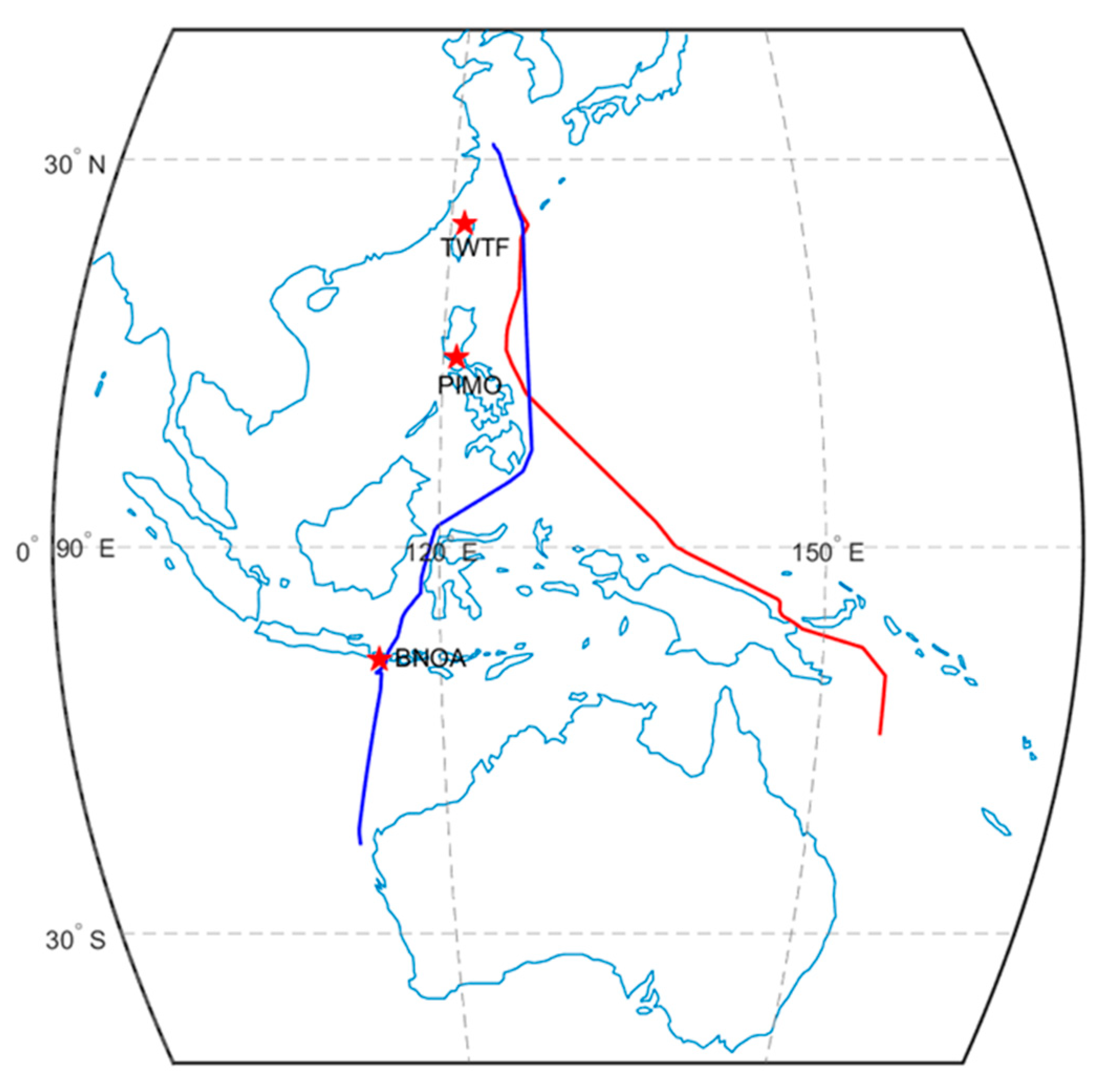
2.1. Kinematic GNSS Data Acquisition

A Chinese research vessel equipped with dual-frequency multi-GNSS receivers was used to collect kinematic data. The receiver Trimble NetR9, with the function of GPS signals tracking and data transmission, which includes pseudorange (C1C and C2W) and carrier-phase measurements (L1C and L2W), and antenna TRM57971.00, were simultaneously utilized. Data in this test is sampled at 30 s. The GNSS data collected on the ships crossing the equator from 31 October to 8 November 2014 (north to south) and from 29 March to 6 April 2015 (south to north) were used to analyze the EIA phenomenon. The experiment was located in the EIA region between 120°E and 150°E. Compared with traditional data, shipborne data has better spatiotemporal resolution, so it can analyze the EIA structure in more detail. Static data from the IGS stations (BNOA, PIMO, and TWTF) near the navigation route in 2015 were also collected for comparison. The route and location of the selected IGS stations are shown in Figure 1.

2.2. Ionosphere TEC Derived from Dual-Frequency GNSS Observations

A carrier-phase smoothed pseudorange method was adopted in this study to quantify the ionospheric Total Electronic Content (TEC) derived from L1 and L2 GNSS observations. The TEC can be calculated with the following equation [26,27,31,32]:

$$P_1-P_2=\frac{40.3(f_2^2-f_1^2)}{f_1^2{f}_2^2}\text{·}F(\alpha )\text{·}\mathrm{VTEC}-c({\mathrm{DCB}}_{\mathrm{s}}{+\mathrm{DCB}}_{\mathrm{r}})$$

(1)

where P₁ and P₂ are the pseudoranges at the L1 and L2 frequencies, respectively; f₁ and f₂ are the L1 and L2 frequencies for each GNSS constellation, respectively; F(α) represents the projection function in the Ionospheric pierce point (IPP), playing the role of converting the ionospheric TEC value direction to the ionospheric VTEC value (the function is largely contingent on α, which is the zenith angle between the ionospheric pierce point and the satellite, and ${\mathrm{DCB}}_{\mathrm{s}}$ is the differential code biases for the satellites, while ${\mathrm{DCB}}_{\mathrm{r}}$ represents the differential code biases for a receiver; c is the speed of light in a vacuum.

Some big errors in the calculated ionospheric TEC values may be caused by incorrect DCB_s of the satellite and receiver. The generalized trigonometric series function (GTSF), which evaluated the single-day DCB of the receiver as a constant, was used to describe the ionospheric variation patterns above the GNSS stations to be monitored. How precisely to determine the ionospheric TEC using the GTSF model is discussed in detail in references [15,28,29,33]:

$$\mathrm{VTEC}\left(\phi ,\lambda \right)={\displaystyle \sum _{n=0}^{n_{max}}{\displaystyle \sum _{m=0}^{m_{max}}\left\{E_{nm}{\phi }^n{h}^m\right\}}}+{\displaystyle \sum _{k=0}^{k_{max}}\{C_k\cos (k\cdot h)}+S_k\sin (k\cdot h)\}$$

(2)

where $\mathrm{VTEC}\left(\phi ,\lambda \right)$ is the VTEC value at the intersect pierce point; $\phi$ and $\lambda$ are the latitude and longitude for the ionospheric pierce point, respectively; h is the function dependent upon the standard time t at the ionospheric pierce point; $n_{max}$ and $m_{max}$ are the maximum orders of the polynomial function, while $k_{max}$ is the maximum order for the trigonometric function; and $E_{nm}$, $C_k$, and $S_k$ are the coefficients to be estimated from the model. Without the fixed middle latitude of regional center, the function can be used to model the variation of ionospheric TEC in a kinematic case, and the receiver DCBs are considered as constant parameters during one day. It should be pointed out that the satellite DCBs are corrected by the product from CAS (ftp.gipp.org.cn, accessed on 30 July 2021).

2.3. Comparison of Different Satellite System Combinations

The VTEC of each satellite IPP point observed simultaneously is calculated by the height angle weighted average to obtain the VTEC of the receiver zenith direction. Figure 2 shows the zenith direction VTEC obtained from the different combinations of satellite systems in 2015, with a time resolution of 30 s (In our analysis, the C1C and C2C measurements of GLONASS are used, while the C2I and C7I measurements of BeiDou are used.). As the number of satellites observed simultaneously increases, the observation data of satellites with high-altitude angles increase. This increases the consistency of the VTEC in the receiver zenith direction with that of the real situation, making the receiver zenith direction VTEC obtained by different combinations of the satellite system more accurate.

In our experiment, the ionospheric TEC information was extracted from the shipborne GNSS observation data for ten days from 29 March to 7 April 2015 according to the method of the carrier-phase smoothing pseudorange, which is the TEC in the line-of-sight direction—that is, STEC. Then, a generalized trigonometric series function was used to model the variation of local ionospheric TEC, while the receiver DCBs are estimated and the satellite DCBs are corrected by prior values from the CAS DCB product.

After removing the DCB errors, it can be transformed from Equation (1) into the new equation below:

$$\mathrm{TEC}=\frac{f_1{}^2{f}_2{}^2}{40.3\left(f_2{}^2-f_1{}^2\right)}\left[ \left({\tilde{P}}_1-{\tilde{P}}_2\right)-c\ast \left({\mathrm{DCB}}_{\mathrm{s}}+{\mathrm{DCB}}_{\mathrm{r}}\right)\right]$$

(3)

where ${\tilde{P}}_1$ and ${\tilde{P}}_2$ are the phase-smoothed pseudoranges.

It is converted to VTEC by the trigonometric projection function, and the VTEC of each satellite puncture point observed at each time is obtained by the weighted average of the height angle of the puncture point to obtain the VTEC in the direction of the zenith of the receiver, and the time series diagram of the VTEC is drawn, as shown in Figure 2.

It can be seen from the aforementioned discussions that the biases for different satellite systems, i.e., the receiver and satellite DCBs, have been precisely corrected from the raw ionospheric TEC observables, and the consistency of the ionospheric TEC extracted from different satellite systems is very good.

3. Results and Analysis

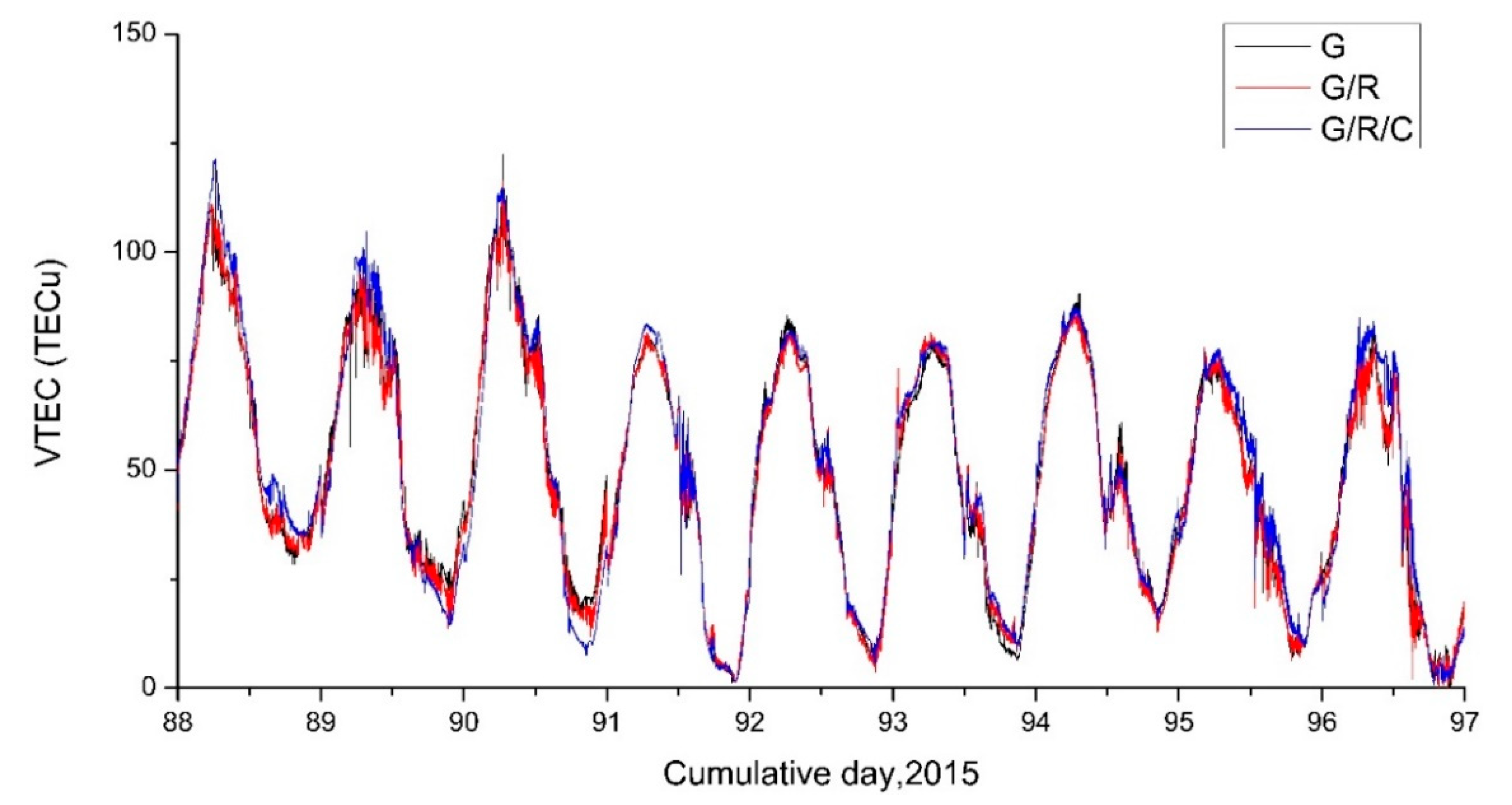
3.1. Comparison of Different Satellite System Combinations

The accuracy of the shipboard kinematic-derived ionospheric TEC was verified by the static one obtained from the IGS-based stations. Figure 3 demonstrates the variations of two TECs over time in 2015. The resemblance in shape and magnitude between the ionospheric TECs when the location of the ship and an IGS station were in proximity proved the reliability of the kinematic ionospheric TEC data. However, the ground-based stations can only observe the change in VTEC statically, which is spatially limited. The scarcity of ocean regional observation stations has magnified this disadvantage, leading to a large area of the ocean surface that cannot obtain the ionosphere TEC calculated using ground-based station data. The shipborne GNSS data exhibited good spatiotemporal continuity. The spatiotemporal characteristics of the EIA phenomenon can be analyzed in more detail.

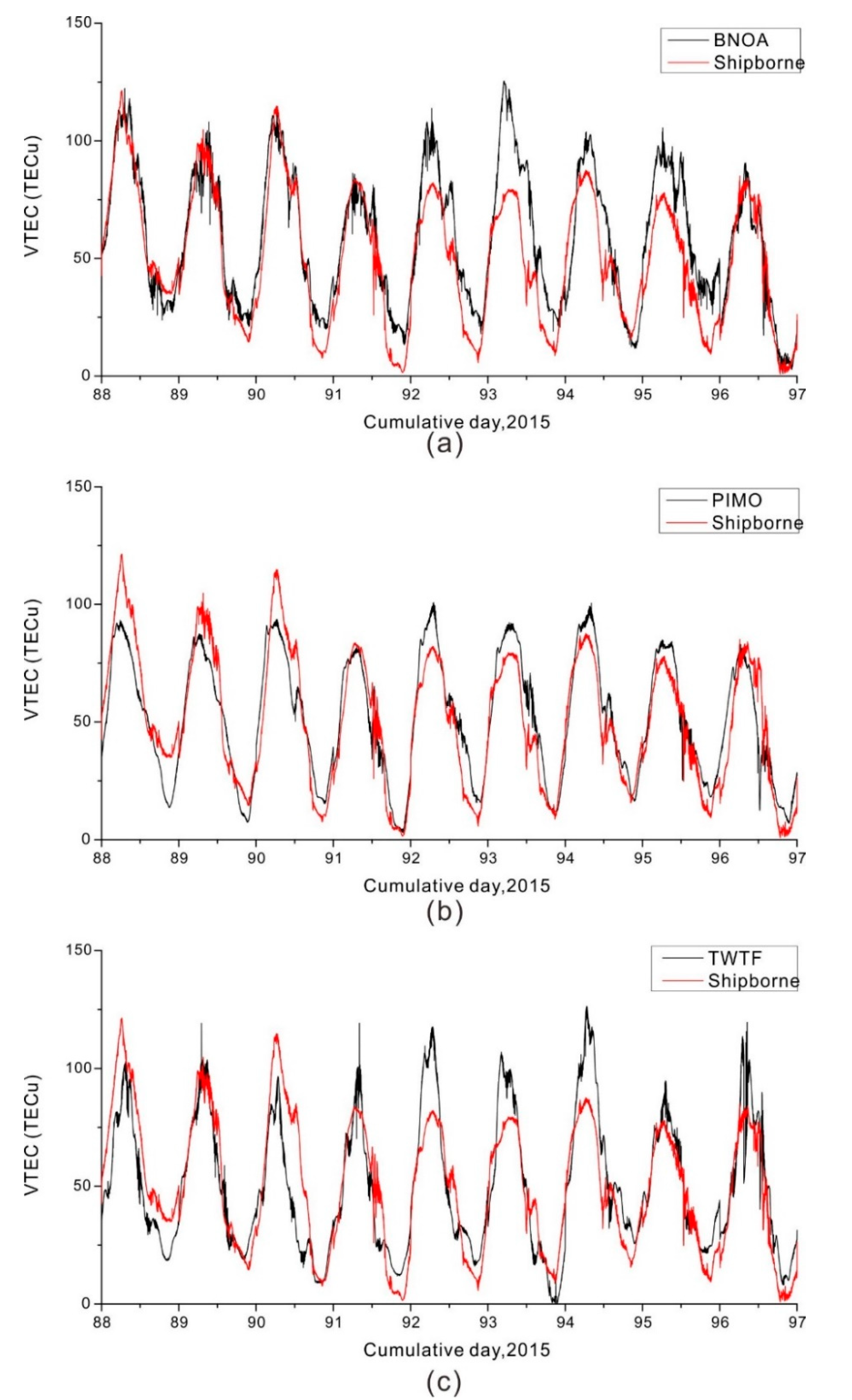
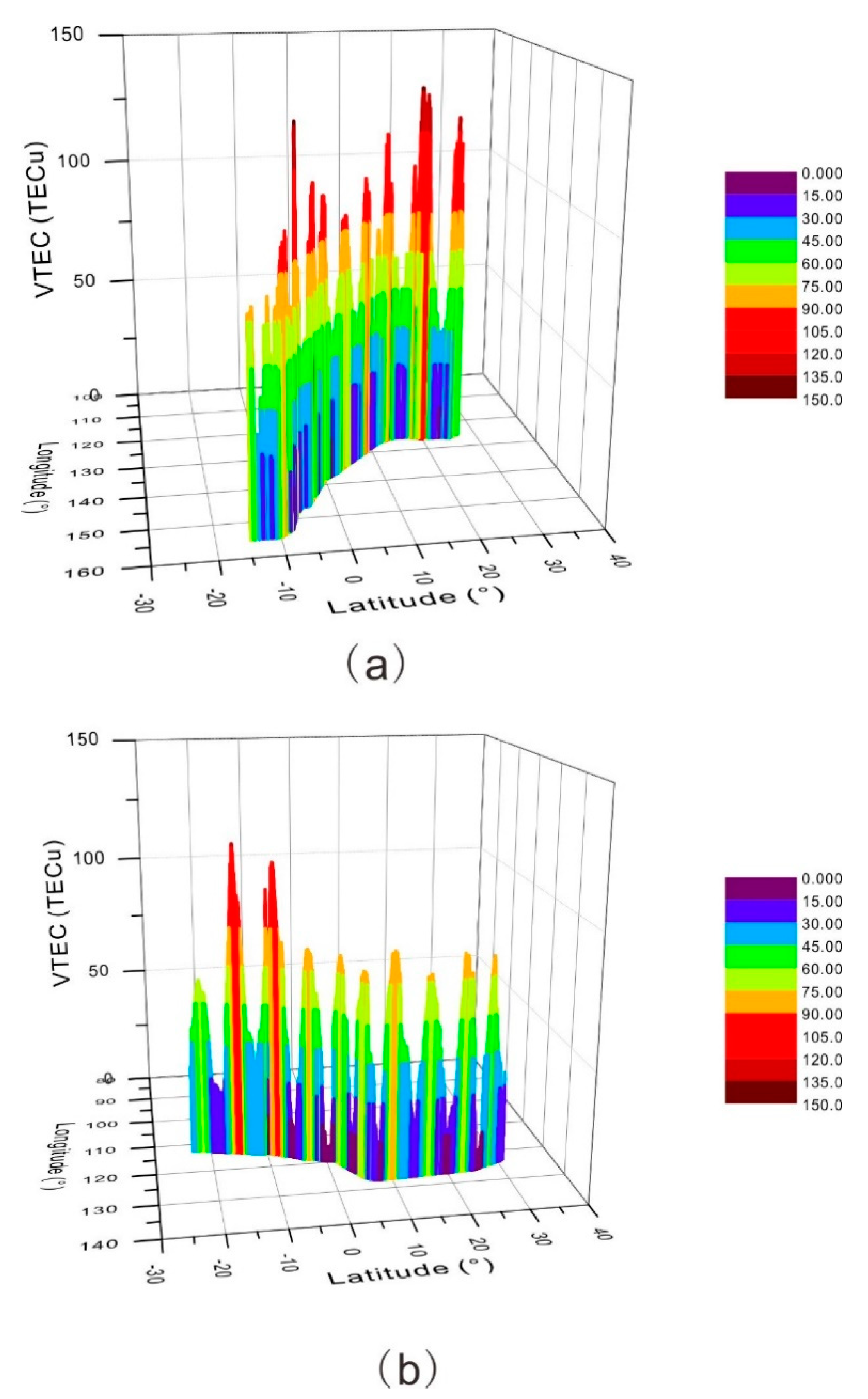
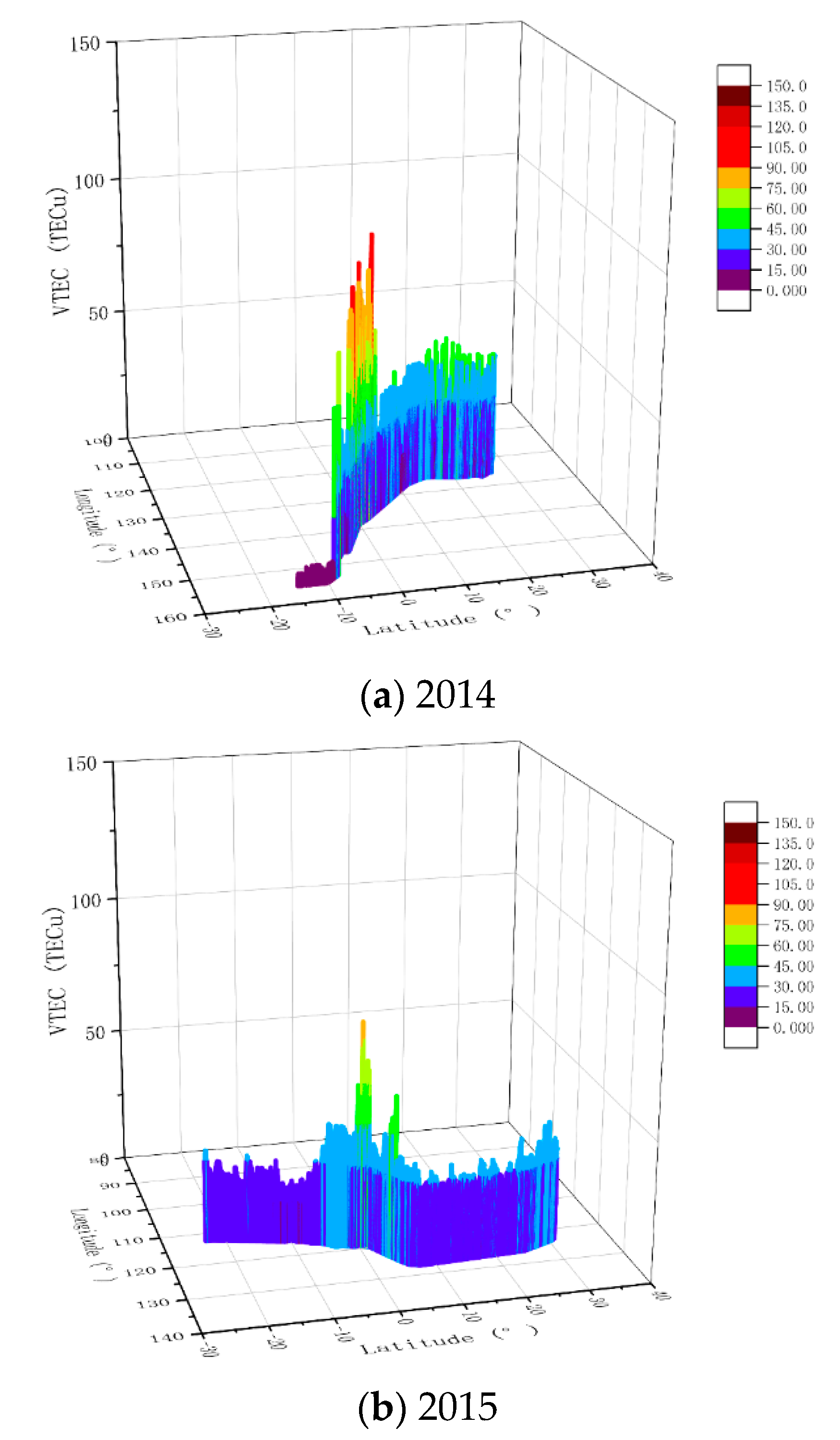
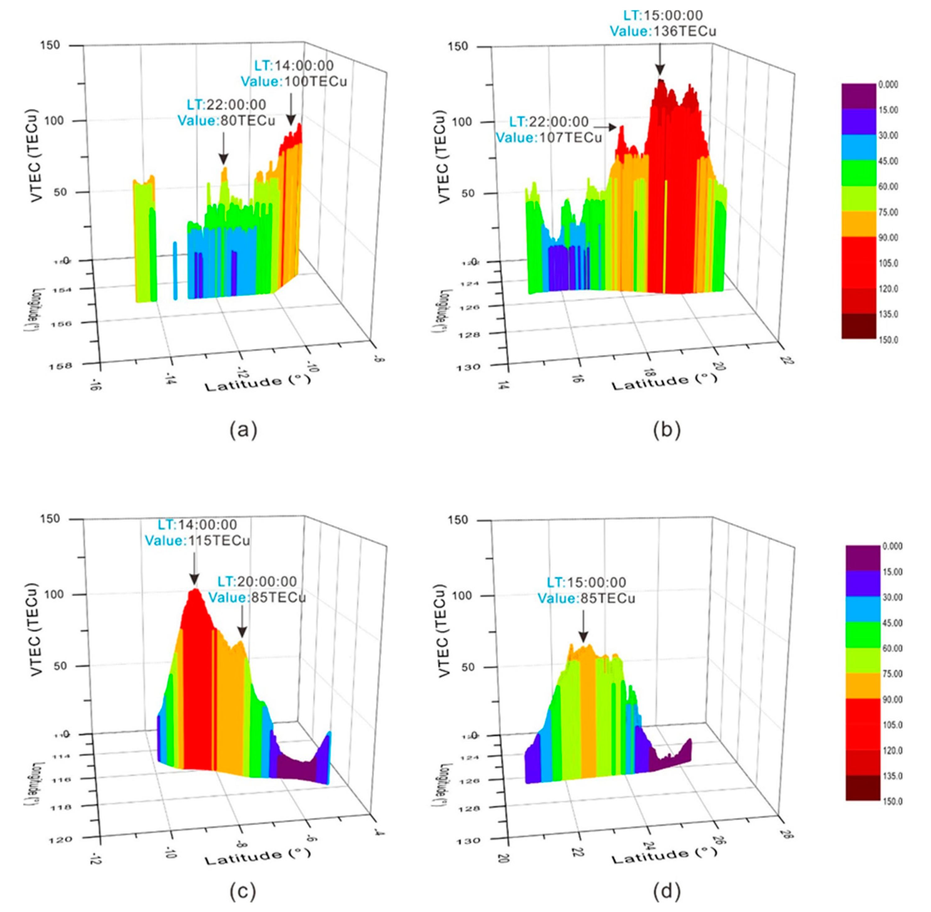
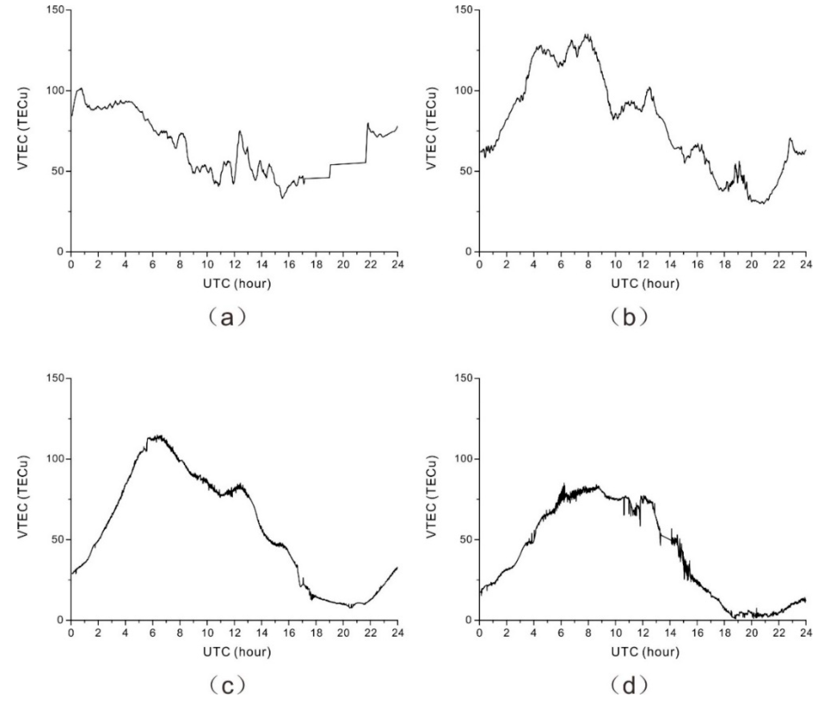
3.2. Analysis of Spatiotemporal Characteristics of Kinematic Ionospheric TEC

In order to enhance the analysis of the spatiotemporal attributes of the EIA over the ocean, the two-year kinematic ionospheric TEC with latitude and longitude was graphed (Figure 4). In this study, we define March–May as the spring and September–November as the autumn. It can be seen from Figure 4 that the ionospheric TEC of the EIA region in (a) is higher than that in (b). Meanwhile, the ionospheric TEC in the Northern Hemisphere in the autumn is generally higher than that in the Southern Hemisphere, while the ionospheric TEC in the Southern Hemisphere in the spring is generally higher than that in the Northern Hemisphere. The preliminary analysis showed that the intensity of the EIA in the autumn is higher than that in the spring, and the EIA phenomenon in this area is asymmetrical between the Northern and Southern Hemispheres. The intensity of the EIA in the Northern Hemisphere in the autumn is greater than that in the Southern Hemisphere, and the intensity of the EIA in the Southern Hemisphere in the spring is greater than that in the Northern Hemisphere, and the EIA changes more drastically in the autumn.

These results are in line with the conclusions obtained in many of the previous studies mentioned in the Introduction section by analyzing the data of the land-based stations—that is, the EIA phenomenon has asymmetry between the Northern and Southern Hemispheres and an obvious seasonal change law, which shows the feasibility of analyzing EIA phenomenon by shipborne dynamic data.

The changes of dynamic ionospheric TEC with the latitude and longitude calculated from the shipborne data indicated that the EIA phenomenon presents a strong asymmetry between the Northern and Southern Hemispheres, and the specific manifestation is that the positions and sizes of the peaks appearing in the Northern and Southern Hemispheres are inconsistent. The peak of the EIA phenomenon in this area is around 20°N in the Northern Hemisphere and around 10°S in the Southern Hemisphere. In the spring, the peak value of the EIA phenomenon in the Southern Hemisphere is higher than that in the Northern Hemisphere, and in the autumn, the peak value of the EIA phenomenon in the Northern Hemisphere is higher than that in the Southern Hemisphere.

As shown in Figure 5, the equatorial anomaly calculated by the GIM model also shows that the EIA phenomenon has characteristics of asymmetry between the Northern and Southern Hemispheres [34], but compared to the actual measurements, the peak is between 0° and 10° on both hemispheres. In addition, it also shows the inconsistency of the peak values of the EIA phenomenon in the Northern and Southern Hemispheres.

To study the regional EIA phenomenon more comprehensively, the four days of November 1 and 8 in 2014 and 31 March and 6 April in 2015 were selected for a specific analysis. Figure 6 and Figure 7 were plotted, and through the analysis, the following conclusions were obtained. During the test of 2014, the two maximums of the EIA phenomenon in both hemispheres appeared at approximately LT14:00 (100TECu) and LT22:00 (80TECu) and at approximately LT15:00 (136TECu) and LT22:00 (107TECu), respectively. During the test of 2015, the EIA phenomenon had two maximums: LT14:00 (~115TECu) and LT20:00 (~85TECu) in the Southern Hemisphere. In the Northern Hemisphere, only a maximum of about 85TECu appeared at LT15:00. Based on a summary of the analysis above, it was concluded that the hemispheres’ asymmetry of the EIA phenomenon has seasonal variations.

4. Conclusions

This paper used shipborne multi-GNSS kinematic data to obtain the equatorial ionospheric TEC in the Western Pacific Ocean. The spatiotemporal characteristics of the EIA phenomenon in this region were analyzed. The ionosphere TEC obtained by the ground-based stations was discrete, while that from the shipborne kinematic data had spatiotemporal continuity, which was favorable in the fine analysis of the EIA.

Based on the high spatiotemporal resolution data of 2014 and 2015, the diurnal variation and the hemisphere asymmetry of the EIA phenomenon between 120°E and 150°E of the Western Pacific Ocean were analyzed comprehensively. The intensity and occurrence time of the maximum of the EIA phenomenon in the Northern and Southern Hemispheres were different during the test. In 2014, the Northern Hemispheric maximum levels of 136TECu and 107TECu appeared at LT15:00 and LT22:00, respectively. The maximums of the Southern Hemisphere appeared at about LT14:00 and LT22:00, and the magnitudes were approximately 100TECu and 80TECu, respectively. In 2015, the Northern Hemispheric crest weakened, and only one maximum appeared at about LT15:00 with a magnitude about 85TECu. The maximums appeared in the Southern Hemisphere at LT14:00 and LT20:00, and the magnitudes were about 115TECu and 85TECu, respectively. The EIA phenomenon in both hemispheres exhibited strong hemisphere asymmetry.

Future research studies will involve the collection of more shipborne data to analyze the interannual variability of the EIA phenomenon in the marine region and fill the gaps in ionosphere research. The relationship between the ionosphere TEC and geographic location in the equatorial region could also be investigated.

References

1. Appleton, E.V. Two Anomalies in the Ionosphere. Nat. Cell Biol. 1946, 157, 691. [Google Scholar] [CrossRef]
2. Croom, S.; Robbins, A.; Thomas, J.O. Two Anomalies in the Behaviour of the F2 Layer of the Ionosphere. Nat. Cell Biol. 1959, 184, 2003–2004. [Google Scholar] [CrossRef]
3. Hanson, W.B.; Moffett, R.J. lonization transport effects in the equatorialFregion. J. Geophys. Res. Space Phys. 1966, 71, 5559–5572. [Google Scholar] [CrossRef]
4. Gadsden, M. An Introduction to the Ionosphere and Magnetosphere. Phys. Bull. 1973, 24, 448. [Google Scholar] [CrossRef]
5. Martyn, D.F. Theory of height and ionization density changes at the maximum of a Chapman-like region, taking account of ion production, decay, diffusion and tidal drift. In Proceedings of the Physics of the Ionosphere, Cavendish Laboratory, Cambridge, UK, September 1954; The Physical Society: London, UK, 1955; p. 254. [Google Scholar]
6. Sethia, G.; Chandra, H.; Rastogi, R.G. Equatorial electrojet control on the low latitude ionospheric total electron content. Proc. Indian Acad. Sci. Sect. A 1979, 88, 87–91. [Google Scholar]
7. Townsend, R.E.; Cannata, R.W.; Prochaska, R.D.; Rattray, G.E.; Holbrook, J.C. Source Book of the Solar-Geophysical Environment. Air Force Glob. Weather. Cent. Offutt Afb Ne 1982. [Google Scholar]
8. Richmond, A.D. Modeling the ionosphere wind dynamo: A review. Pure Appl. Geophys. 1989, 131, 413–435. [Google Scholar] [CrossRef]
9. Balan, N.; Bailey, G.J.; Abdu, M.A.; Oyama, K.I.; Richards, P.G.; MacDougall, J.; Batista, I.S. Equatorial plasma fountain and its effects over three locations: Evidence for an additional layer, the F3 layer. J. Geophys. Res. Space Phys. 1997, 102, 2047–2056. [Google Scholar] [CrossRef]
10. Venkatesh, K.; Fagundes, P.R.; Prasad, D.S.V.V.D.; Denardini, C.M.; De Abreu, A.J.; De Jesus, R.; Gende, M. Day-to-day variability of equatorial electrojet and its role on the day-to-day characteristics of the equatorial ionization anomaly over the Indian and Brazilian sectors. J. Geophys. Res. Space Phys. 2015, 120, 9117–9131. [Google Scholar] [CrossRef] [Green Version]
11. Kumar, S.; Patel, K.; Singh, A.K. TEC variation over an equatorial and anomaly crest region in India during 2012 and 2013. GPS Solut. 2015, 20, 617–626. [Google Scholar] [CrossRef]
12. Klobuchar, J.A. Ionospheric Time-Delay Algorithm for Single-Frequency GPS Users. IEEE Trans. Aerosp. Electron. Syst. 1987, AES-23, 325–331. [Google Scholar] [CrossRef]
13. Yuan, Y.; Ou, J. Auto-covariance estimation of variable samples (ACEVS) and its application for monitoring random ionospheric disturbances using GPS. J. Geod. 2001, 75, 438–447. [Google Scholar] [CrossRef]
14. Prieto-Cerdeira, R.; Orús-Pérez, R.; Breeuwer, E.; Lucas-Rodriguez, R.; Falcone, M. Performance of the Galileo single-frequency ionospheric correction during in-orbit validation. GPS World 2014, 25, 53–58. [Google Scholar]
15. Li, Z.; Yuan, Y.; Wang, N.; Hernandez-Pajares, M.; Huo, X. SHPTS: Towards a new method for generating precise global ionospheric TEC map based on spherical harmonic and generalized trigonometric series functions. J. Geod. 2015, 89, 331–345. [Google Scholar] [CrossRef]
16. Yuan, Y.; Wang, N.; Li, Z.; Huo, X. The BeiDou global broadcast ionospheric delay correction model (BDGIM) and its preliminary performance evaluation results. Navigation 2019, 66, 55–69. [Google Scholar] [CrossRef] [Green Version]
17. Xu, Z.; Wang, W.-M.; Wang, B.; Yang, S.-G. Analysis and prediction of ionospheric total electron content of the Equatorial Ionization Anomaly around 120°E longitude. Chin. J. Geophys. 2012, 7, 2185–2192. [Google Scholar]
18. Kumar, S.; Priyadarshi, S.; Krishna, S.G.; Singh, A.K. GPS-TEC variations during low solar activity period (2007–2009) at Indian low latitude stations. Astrophys. Space Sci. 2012, 339, 165–178. [Google Scholar] [CrossRef]
19. Ouattara, F.; Gnabahou, D.A.; Mazaudier, C.A. Seasonal, Diurnal, and Solar-Cycle Variations of Electron Density at Two West Africa Equatorial Ionization Anomaly Stations. Int. J. Geophys. 2012, 2012, 1–9. [Google Scholar] [CrossRef]
20. Feng, J.; Wang, Z.; Shi, S.; Zhang, B.B. Using IGS to analyze the variation of anomaly equatorial ionization. Sci. Surv. Mapp. 2016, 41, 44–47. [Google Scholar]
21. Romero-Hernandez, E.; Denardini, C.M.; Takahashi, H.; Gonzalez-Esparza, J.A.; Nogueira, P.A.B.; De Padua, M.B.; Lotte, R.G.; Negreti, P.D.S.; Jonah, O.F.; Resende, L.C.A.; et al. Daytime ionospheric TEC weather study over Latin America. J. Geophys. Res. Space Phys. 2018, 123, 10345–10357. [Google Scholar] [CrossRef]
22. Ram, S.T.; Su, S.-Y.; Liu, C.H. FORMOSAT-3/COSMIC observations of seasonal and longitudinal variations of equatorial ionization anomaly and its interhemispheric asymmetry during the solar minimum period. J. Geophys. Res. Space Phys. 2009, 114, 06311. [Google Scholar] [CrossRef]
23. Huang, L.; Huang, J.; Wang, J.; Jiang, Y.; Deng, B.; Zhao, K.; Lin, G. Analysis of the north–south asymmetry of the equatorial ionization anomaly around 110°E longitude. J. Atmos. Sol. Terr. Phys. 2013, 102, 354–361. [Google Scholar] [CrossRef]
24. Walker, G.O.; Ma, J.H.K.; Golton, E. The equatorial ionospheric anomaly in electron content from solar minimum to solar maximum for South East Asia. Ann. Geophys. 1994, 12, 195–209. [Google Scholar] [CrossRef]
25. Chen, Y.; Liu, L.; Le, H.; Wan, W.; Zhang, H. Equatorial ionization anomaly in the low-latitude topside ionosphere: Local time evolution and longitudinal difference. J. Geophys. Res. Space Phys. 2016, 121, 7166–7182. [Google Scholar] [CrossRef]
26. Lin, C.H.; Hsiao, C.C.; Liu, J.Y.; Liu, C.H. Longitudinal structure of the equatorial ionosphere: Time evolution of the four-peaked EIA structure. J. Geophys. Res. Space Phys. 2007, 112, 12305. [Google Scholar] [CrossRef]
27. Huang, H.; Lu, X.; Liu, L.; Wang, W.; Li, Q. Transition of Interhemispheric Asymmetry of Equatorial Ionization Anomaly During Solstices. J. Geophys. Res. Space Phys. 2018, 123, 10283–10300. [Google Scholar] [CrossRef]
28. Chou, M.Y.; Lin, C.C.H.; Tsai, H.F.; Lin, C.Y. Ionospheric electron density inversion for Global Navigation Satellite Systems radio occultation using aided Abel inversions. J. Geophys. Res. Space Phys. 2017, 122, 1386–1399. [Google Scholar] [CrossRef]
29. Feng, J.; Han, B.; Zhao, Z.; Wang, Z. A New Global Total Electron Content Empirical Model. Remote Sens. 2019, 11, 706. [Google Scholar] [CrossRef] [Green Version]
30. Lin, C.Y.; Lin, C.C.H.; Liu, T.J.Y.; Rajesh, P.K.; Chou, M.Y. Simulation and Validation of FORMOSAT-7/COSMIC-2 Space Weather Products: Global Iono-spheric Specification Electron Density Structure and Aided Abel Electron Density Profile. In Proceedings of the AGU Fall Meeting Abstracts, San Francisco, CA, USA, 9–13 December 2019; Volume 2019, p. SA13B-3249. [Google Scholar]
31. Yunbin, Y.; Xingliang, H.; Jikun, O. Models and methods for precise determination of Ionospheric delay using GPS. Prog. Nat. Sci. 2007, 17, 187–196. [Google Scholar] [CrossRef]
32. Wang, C.; Shi, C.; Fan, L.; Zhang, H. Improved Modeling of Global Ionospheric Total Electron Content Using Prior Information. Remote Sens. 2018, 10, 63. [Google Scholar] [CrossRef] [Green Version]
33. Yuan, Y.; Ou, J. A generalized trigonometric series function model for determining ionospheric delay. Prog. Nat. Sci. 2004, 14, 1010–1014. [Google Scholar] [CrossRef]
34. Yuan, Y. Study on the New Methods of Correcting Ionospheric Delay and Ionospheric Model Using GPS Data. J. Grad. Sch. Chin. Acad. Sci. 2002, 19, 209–214. [Google Scholar]
Figure 1. Routes of the Chinese research vessel in 2014 (red line) and 2015 (blue line), and locations of the selected IGS stations.
Remotesensing 13 03051 g001
Figure 2. Receiver zenith direction VTEC obtained through different combinations of satellite systems (G: GPS, R: GLONASS, and C: BDS) in 2015.
Remotesensing 13 03051 g002
Figure 3. Comparison of ionospheric VTEC values for the kinematic (shipborne) data and static data for the IGS stations.
Remotesensing 13 03051 g003
Figure 4. Variations of shipboard kinematic ionospheric TEC with latitude and longitude: (a) 2014 and (b) 2015.
Remotesensing 13 03051 g004
Figure 5. The change of ionospheric TEC calculated by the GIM model with the latitude and longitude (The ionospheric change at the same latitude and longitude calculated from the measured data).
Remotesensing 13 03051 g005
Figure 6. Comparison of ionospheric changes over the latitude and longitude in the Northern and Southern Hemispheres: (a) 8 November 2014, (b) 1 November 2014, (c) 31 March 2015, and (d) 6 April 2015.
Remotesensing 13 03051 g006
Figure 7. Comparison of the ionospheric changes over time in the Northern and Southern Hemispheres: (a) 8 November 2014, (b) 1 November 2014, (c) 31 March 2015, and (d) 6 April 2015.
Remotesensing 13 03051 g007
Publisher’s Note: MDPI stays neutral with regard to jurisdictional claims in published maps and institutional affiliations.