
Domain Adaptive Ship Detection in Optical Remote Sensing Images


1
School of Automation, Beijing Institute of Technology, Beijing 100081, China
2
State Key Laboratory of Advanced Power Transmission Technology, Global Energy Interconnection Research Institute Co., Ltd., Beijing 102209, China
*
Author to whom correspondence should be addressed.
Remote Sens. 2021, 13(16), 3168; https://0-doi-org.brum.beds.ac.uk/10.3390/rs13163168
Submission received: 3 July 2021
/
Revised: 5 August 2021
/
Accepted: 9 August 2021
/
Published: 10 August 2021
(This article belongs to the Special Issue Computer Vision and Deep Learning for Remote Sensing Applications)
Abstract
:With the successful application of the convolutional neural network (CNN), significant progress has been made by CNN-based ship detection methods. However, they often face considerable difficulties when applied to a new domain where the imaging condition changes significantly. Although training with the two domains together can solve this problem to some extent, the large domain shift will lead to sub-optimal feature representations, and thus weaken the generalization ability on both domains. In this paper, a domain adaptive ship detection method is proposed to better detect ships between different domains. Specifically, the proposed method minimizes the domain discrepancies via both image-level adaption and instance-level adaption. In image-level adaption, we use multiple receptive field integration and channel domain attention to enhance the feature’s resistance to scale and environmental changes, respectively. Moreover, a novel boundary regression module is proposed in instance-level adaption to correct the localization deviation of the ship proposals caused by the domain shift. Compared with conventional regression approaches, the proposed boundary regression module is able to make more accurate predictions via the effective extreme point features. The two adaption components are implemented by learning the corresponding domain classifiers respectively in an adversarial training way, thereby obtaining a robust model suitable for both of the two domains. Experiments on both supervised and unsupervised domain adaption scenarios are conducted to verify the effectiveness of the proposed method.
1. Introduction
The technique of ship detection can find a wide range of applications in both military and civilian fields, and has received extensive attention from researchers for a long time. In recent years, encouraged by the great success of convolutional neural network (CNN)-based object detection methods [1,2,3,4,5,6,7,8,9,10], many researchers propose to utilize a similar methodology for ship detection in optical remote sensing images [11,12,13,14,15,16,17,18].
Following the pipeline of general object detection algorithms, these methods can be divided into two categories of region-based methods and regression-based methods. The region-based methods first generate a set of region proposals based on predefined anchor boxes via the region proposal network (RPN) [5]. Then, those candidate regions are refined to obtain the final detection results [11,12,14,15,16]. In contrast, regression-based methods directly regress the bounding box of each object from different locations [13,17,18]. In general, the region-based methods have higher detection accuracy, while regression-based methods run faster. With the help of the powerful feature extraction ability of CNN, these methods achieves promising improvements compared with their traditional counterparts which relies on manually designed features for the detection.
Despite the effectiveness of these CNN-based ship detection methods, they are only trained and tested on a single domain (dataset). In practical applications, the changing environments and weather conditions often lead to large domain shift between different domains. Such domain shift commonly exists in object detection tasks and has been observed to cause significant performance drop when apply the trained model to a visually different new domain [19]. Therefore, to improve the detection performance on both of the two domains, a natural idea is to train on the two domains together to cover richer situations. However, without dedicated treatments, the model will tend to fit the two domains with sub-optimal feature representations separately, and thus leads to inferior detection results.
To solve this problem, we propose a novel domain adaptive ship detection method based on the region-based detection pipeline. The basic idea is to minimize the distance of the feature distribution between the two domains on both image-level and instance-level. In general, this distance is usually optimized by maximizing the error rate of the domain classifier that predicts the domain label of the data [20,21,22]. Moreover, conventional feature extraction networks are employed for typical single-domain object detection. These networks are less powerful to deal with the large domain shift between different domains in remote sensing images. Therefore, some innovative treatments are also proposed for better feature representation between different domains.
In image-level adaption, several improvements are proposed to overcome the shortcomings of conventional feature extraction networks for the overall image feature extraction. Specifically, we reasonably integrate the feature maps with different receptive fields via the attention-based feature fusion structure. In this way, the integrated feature map is able to better perceive ships of different sizes on each pixel location. Then, the feature map is optimized in the channel direction for more suitable cross-domain feature representations based on the squeeze-and-excitation (SE) [23] mechanism, which emphasizes important features by modelling the interdependencies between different channels of the feature map. Finally, the optimized feature maps are fed into the domain classifier to obtain aligned feature representations between the two domains.
In addition to the overall image-level features, the domain shift also affects instance-level feature expression, which leads to deviations in object localization. Therefore, to obtain more accurate detection results, we propose the boundary regression module to refine the region proposals generated by RPN. The proposed module utilizes extreme point features closest to the boundary of the proposal to predict the offset of each corresponding boundary. Compared with the traditional bounding box regression approach, the boundary regression module discards redundant features useless for object localization, making the regression process more robust and accurate. Similar to image-level adaption, the domain classifier is also used to align the refined region of interest (ROI) features. Moreover, the proposed module is also suitable for the unsupervised domain adaption scenario, where the bounding box annotations are only available in one of the two domains.
2. Related Work
2.1. General Object Detection
In recent years, convolutional neural networks (CNN) have shown powerful abilities in various visual tasks such as image classification [24,25,26], semantic segmentation [27,28,29] and object detection. In general, current CNN-based object detection methods can be divided into two categories. The first category generates a series of region proposals via the region proposal network (RPN) [5] or selective research [1] at first. Then, on each proposal, region classification and bounding box regression are performed to obtain the final detection results [1,2,3,4,5,6,7,9,10]. Among all these methods, Faster R-CNN [5] is the most representative one, which integrates all these steps into a unified network for the first time.
The second category directly obtains the object bounding boxes from predefined default boxes via regression, ignoring the process of proposal generation. For example, the single-shot multibox detector (SSD) [3] predicts bounding box offsets and probability scores for the densely distributed default boxes based on the feature maps of different scales. In pursuit of faster running speed, you only look once (YOLO) [2] divides the image into several grids. Then, two default boxes are defined at the center location of each grid to perform region classification and regression. Although these one-step methods usually have inferior detection performance than those proposal-based ones, YOLOv3 [9] (the upgradation version of [6]) still achieves impressive performance with the help of multiple improvements.
2.2. Ship Detection in Optical Remote Sensing Images
Ship detection is a hot research topic in the fields of remote sensing. The manually-designed features (such as geometric elements) are widely used in early ship detection methods to identify ships from the background. For instance, Lei et al. [30] and Lin et al. [31] perform onshore ship detection via the contour feature and line segment. A hierarchical complete and operational ship detection method was proposed in [32] based on shape and texture features. Since these basic geometric features are not robust enough in complex background interference, more prominent features of the ship head are used in some other methods for preliminary localization. In [33], the regions of potential ship heads are first predicted by transforming local pixels into the polar coordinate system, based on which the saliency of directional gradient information is then employed to identify ship body. The ship heads are detected in [34] by corner features, and then the methods of shape analysis and region growth are used to determine the complete ship region. The method [35] first determines the potential ship regions by saliency segmentation, and then the structure-LBP features are used to identify the real ships. However, these manually-designed features can only utilize low-level information with poor generalization ability, these methods often suffer from the influence of complex background, resulting in either false or miss detection.
In recent years, based on the successful CNN-based object detection methods, many similar ship detection algorithms in optical remote sensing images are proposed and achieve good results [11,12,13,14,15,16,17,18]. Li et al. [11] detect ships of various scales via the multi-scale feature mapping. Nie et al. [12] improve the post-processing process of the Mask R-CNN [10] algorithm and use it for ship detection. Zhang et al. [15] rotate the ship candidate regions to achieve arbitrarily oriented ship detection. Li et al. [16] propose a novel dual-branch regression network to more effectively predict the ship orientation and other variables independently. For the regression-based methods, Liu et al. [13] pass through shallow layer feature maps to deeper ones to utilize fine-grained features for small ship detection. Based on the advanced YOLOv3, Chen et al. [18] propose a lightweight dilated attention module to achieve a trade-off between detection accuracy and speed. However, these methods are all trained and tested on a single dataset with simple scenarios, which have limited generalization abilities in practical applications.
2.3. Domain Adaption
The purpose of domain adaption is to find a domain-invariant feature representation to achieve information transfer. Various methods have been proposed to solve this problem in computer vision, such as image classification and semantic segmentation [36,37,38,39]. Recently, inspired by the powerful generative adversarial network (GAN) [40], adversarial learning is widely used to align features between different domains. For example, Ganin et al. [37] effectively improve the performance of the domain adaptive classification task via the domian classifier and a gradient reversal layer. Tzeng et al. [38] propose an adversarial discriminative domain adaption model, which combines the discriminative model, untie weight sharing, and GAN loss for classification. With the help of adversarial learning, Tsai et al. [39] achieves superior performance in domain adaptive semantic segmentation.
Recently, some domain adaptive object detection methods have been proposed to solve the problem of cross-domain object detection. Chen et al. [20] optimize the detection model together with the domain classifier by adversarial training to minimize the distance between the features of the two domains. Following the same principle, Saito et al. [21] focus on aligning low-level image features during training, but weakens the alignment of high-level features. To achieve multi-scale feature alignment, Xie et al. [22] set multiple domain classifiers to the middle layers of the feature extraction network for training.
3. The Proposed Method
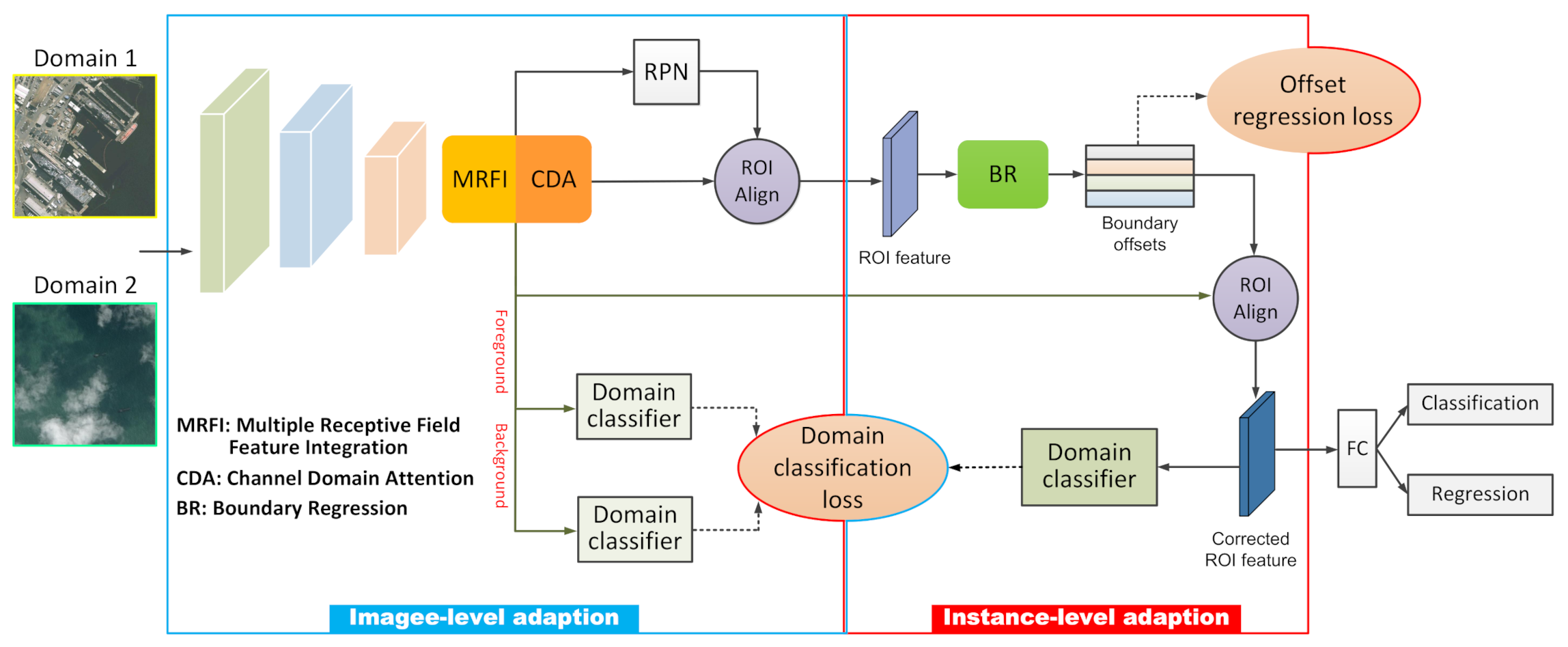
Following the region-based detection pipeline, the overall framework of our method is shown in Figure 1. To achieve the domain adaption based on both image-level and instance-level, some dedicated and innovative structures are used to improve the generalization ability of the detection model. In the following, we will describe them as well as other relevant information of the proposed method in detail.
3.1. Image-Level Adaption
The image-level adaption focuses on coping with the overall image differences through feature alignment. Existing ship detection methods adopt conventional backbone networks for feature extraction. However, the structures of these networks are all designed for single domain and are less powerful to deal with the large domain shift. Therefore, we adopt two successive feature optimization modules to adapt the domain shift in both the width (the receptive field) and depth (the feature channels) direction of the feature map generated by the backbone network. Meanwhile, two independent classifiers are set to align the foreground and background features separately for more effective training.
3.1.1. Multiple Receptive Field Feature Integration
For region-based object detection methods, RPN slides on the feature map via convolutional layers, and predicts classification scores together with bounding box offsets based on the feature vectors which have a fixed receptive field. However, the size of the ship can be arbitrary. It is obviously sub-optimal to predict ships of different sizes with a fixed receptive field. Especially when the domain offset exists, the disharmony between the scale and the receptive field further increases the difficulty of the cross-domain feature representation. To solve this problem, the first step is to enlarge the receptive field of the feature map. A larger receptive field can cover larger objects and contain more context information [41], which is conducive to extracting important features between different domains.
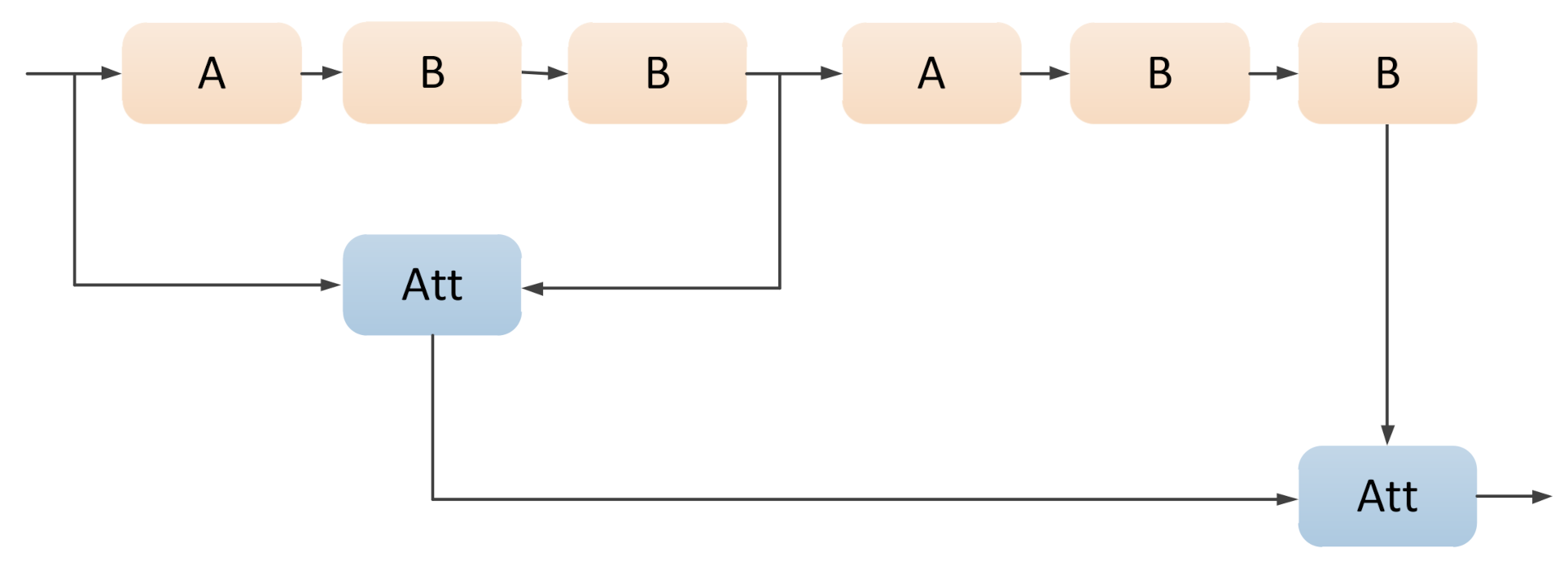
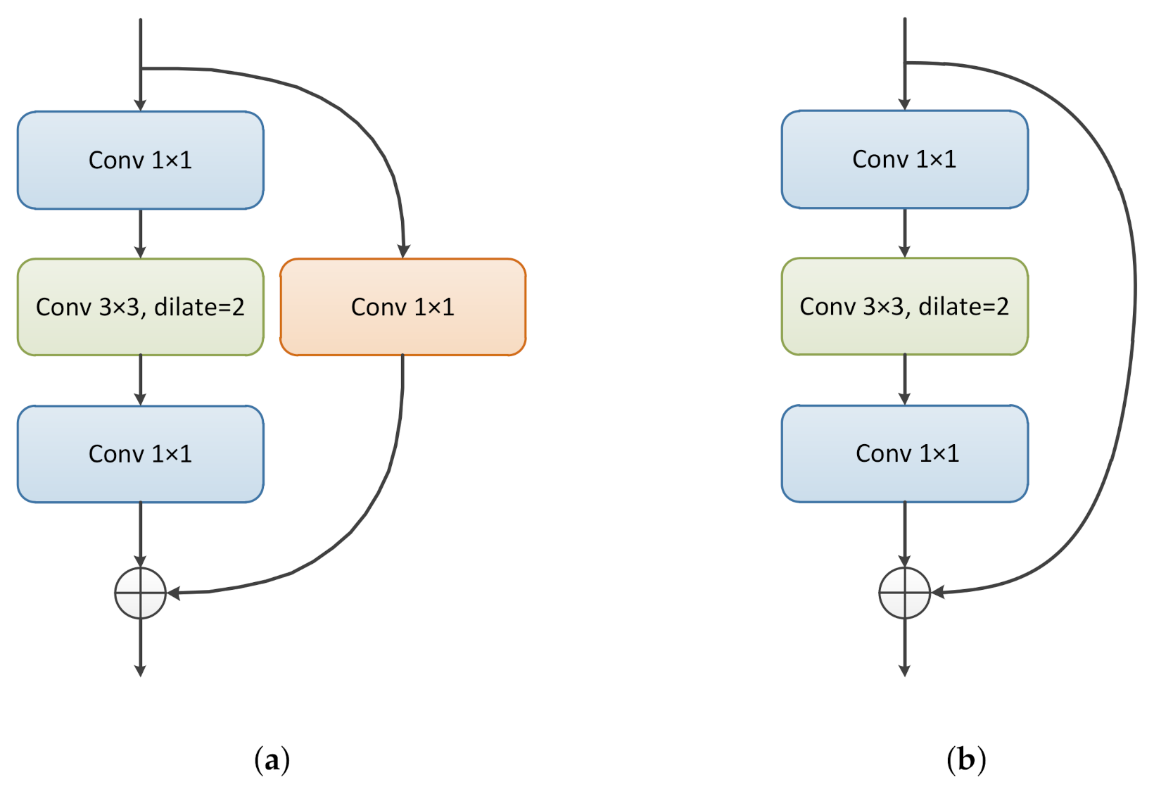
Conventional backbone networks mainly expand the receptive field through the pooling operation [42]. However, pooling is actually a down-sampling process. The loss of the spatial information blurs the boundary of objects, which compromises the object location ability. Therefore, we adopt the dilated convolution to expand the receptive field without down-sampling [43]. Specifically, as shown in Figure 2 and Figure 3, we add the dilated convolution layer to two different types of residual modules, and combine them repeatedly to obtain new feature maps with a larger receptive field [44]. Then, these feature maps should be integrated together to contain multiple pieces of receptive field information. The most common way to merge different feature maps is directly splicing them along the channel. However, due to the semantic gap between different features, this rough combination approach is not conducive to feature learning. Therefore, we gradually integrate the two adjacent feature maps with different receptive fields via a novel attention-based feature fusion module to alleviate the negative impact of the semantic gap (see Figure 2).
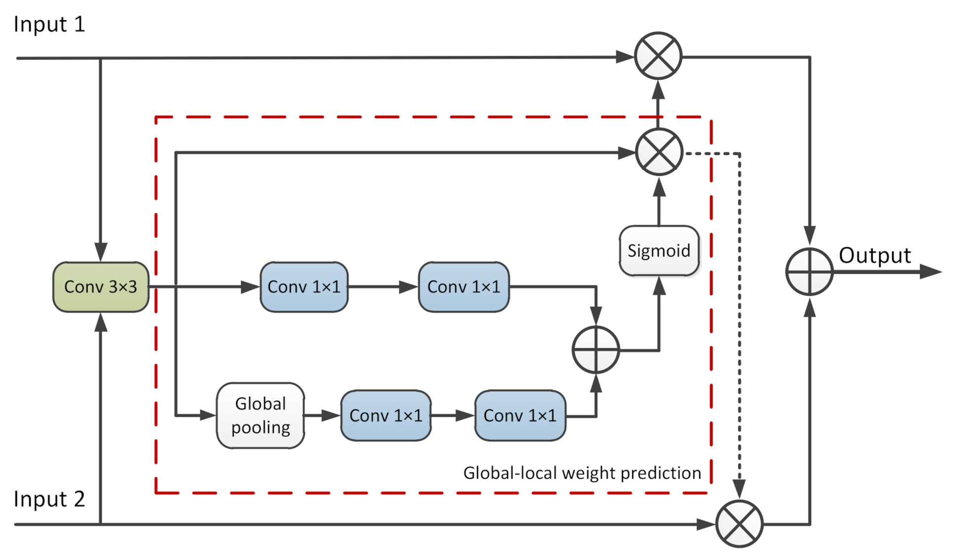
Inspired by [45], the attention-based feature fusion module combines global and local information to predict the weight of the integration. The structure of the attention-based feature fusion is shown in Figure 4, where ⊗ and ⊗ denote element-wise add and multiplication, respectively. Denoting the output of the connected ⊗ as P, then the dotted arrow indicates the operation . The two inputs are first merged together by a convolutional layer after splicing. Then, two parallel convolution branches are used to extract global and local information, respectively. The upper branch is directly calculated on the input feature map to obtain local information, while the lower branch first obtains global information by the global pooling operation. Finally, the outputs of the two branches are element-wise added and passed through the sigmoid activation function to obtain the final fusion weight. Using ⊎ and to represent the convolution operation and global–local weight prediction (the dashed box in Figure 4), respectively, the attention-based feature fusion module can be represented by the following formula:
where and Z represents the two inputs and output, respectively. With the help of the attention-based feature fusion, features with different receptive fields are reasonably integrated to adapt to ship targets of different sizes.
3.1.2. Channel Domain Attention
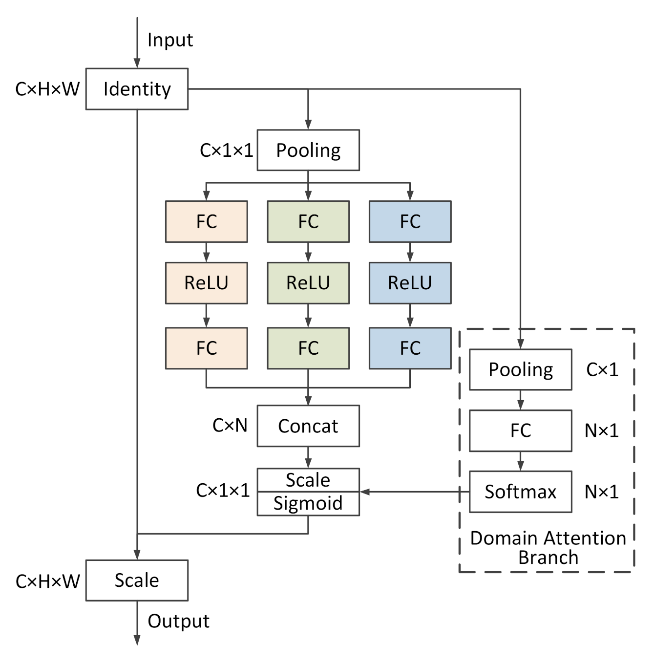
The multiple receptive field feature integration introduced in Section 3.1.1 enables the integrated features to better adapt to the scale changes of ships. However, such location-related optimization is unable to cope with the domain shift caused by environmental and weather changes since these differences are encoded into different feature channels via convolutional layers. One possible solution is to optimize the feature channels to better emphasize the important features of the two domains, while suppressing those that are useless for the feature alignment. Therefore, inspired by the wildly used SE mechanism, we attach the channel domain attention module to multiple receptive field feature integration. The channel domain attention module extends the SE mechanism to different domains, aiming at achieving more effective feature extraction by focusing on individual domains.
The structure of the channel domain attention module is shown in Figure 5, which consists of multiple SE adapters and an attention assignment branch. For a channel domain attention module, the input feature map is first pooled by a global pooling layer to aggregate the spatial information. Then, following the SE mechanism, N SE adapters produce independent channel weights for the C channels of input feature map, selectively emphasising informative features and suppress less useful ones [46]. Next, the attention assignment branch generates domain-specific activations for each SE adapter to obtain the final channel weights. Finally, the input feature map is scaled by the final channel weights through channel-wise multiplication.
The benefit of this module is two-fold: first, the channel-related information is encoded into the output of multiple SE adapters, making the model more sensitive to input changes and easier to capture useful information; second, the attention assignment branch further dynamically integrate these channel-related information for different domains, facilitating the efficacy to obtain robust features suitable for both of the two domains.
3.1.3. Dual Supervision Adaption Approach
Besides the multiple receptive field feature integration and channel domain attention for feature optimization, the domain classifier is also required to achieve cross-domain feature alignment. During training, the domain classifier adjusts its weights to discriminate the domain label of the input features produced by the feature extraction network, while the feature extraction network tries to generate domain-invariant features that can deceive the domain classifier. Therefore, if the classification error is high even for the well-trained domain classifier, it means that the features of the two domains are close to each other. So they are already aligned.
In theory, the image-level adaption should take the output feature map of the feature extraction network as a whole for global feature alignment. However, during training, each activation on the feature map (which represents a fixed-size image patch) is regarded as an independent sample as the input of the domain classifier. The benefits of using image patches instead of the entire image for domain classification are two-fold:
(1) Limited by the computing power, the batch size is usually set to a small value during training. Classifying image patches instead of the whole image can generate more training samples (e.g., 128 per image in our implementation).
(2) Since the classifier requires fixed-size input while the size of the image is changeable, this patch-based classification strategy can avoid the scaling or sampling operation, which will inevitably cause the information distortion.
However, despite of the effectiveness of this patch-based approach, the training samples are dominated by the background since the ship region in remote sensing images only occupies a small part. Therefore, the ship samples will not be fully trained, which is not conducive to obtaining a proper feature representation for the ships between the two domains.
To solve this problem and obtain more effective aligned features, we set two independent domain classifiers of the foreground domain classifier and the background domain classifier to identify the ship samples and background samples from the two domains, respectively (see Figure 1). During training, the classification scores predicted by RPN determine whether current location on the feature map is a ship sample. Specifically, locations with a classification score larger than 0.5 are ship regions, and those with classification scores less than 0.2 are background regions. It is worth noting that to cover different scales and aspect ratios, multiple anchors with different sizes are centred on each location of the feature map. Since each anchor has a corresponding classification score, we take the maximum value as the score of current location.
Specifically, the image-level adaption loss is the sum of the foreground domain classifier and background domain classifier :
We train the domain classifier on each activation located at of the feature map. Denoting the output probability of the domain classifier as p, and is defined as follows:
where denotes the domain label of the i-th training image ( = 0 for the first domain and = 1 for the second domain). for ship samples, or . for background samples, or .
3.2. Instance-Level Adaption
Section 3.1 minimizes the impact of domain shift in terms of the image-level global feature representations. However, images in different domains may also show significant differences in local regions that may contain ships. The feature of these regions also affect the localization accuracy of the detection. Therefore, to achieve local region feature alignment, we design a novel boundary regression module to correct the size and location of the proposals, as well as align the corrected ROI features between different domains via the domain classifier.
Due to the existence of the domain shift, more robust features are required to achieve accurate regression. Although the features in the inside part of the region proposal are helpful for the classification task, they are redundant for the boundary regression and will make the regressor easily affected by the background inference. Therefore, to reduce the interference as much as possible, we only utilize the features closest to the boundary of the proposal for the regression. Such features are the extreme point features with a maximum response value on the boundary of the ROI features.
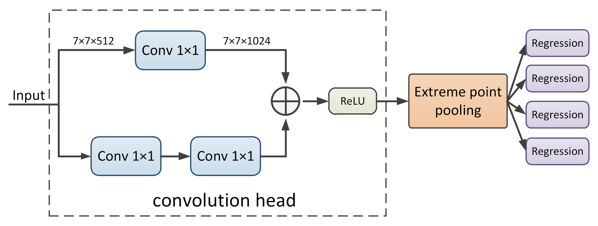
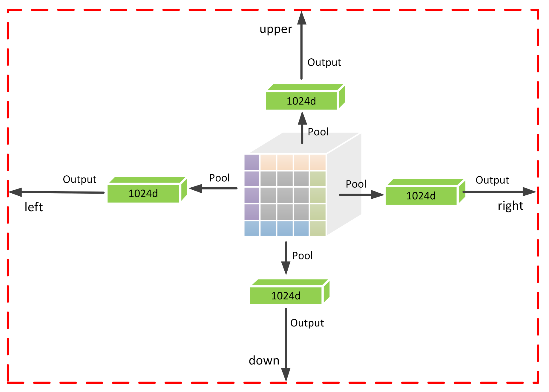
Specifically, as shown in Figure 6, the boundary regression module takes a size feature map produced by the ROI Align [10] layer for each proposal as input. Then, since the convolution operation applies shared transformations which are more robust to regress the ship boundary, the number of channels is increased through two convolution branches to obtain a size feature map. Finally, four 1024-d vectors are obtained via the extreme point pooling to regress the offset of the proposal, respectively. The structure of extreme point pooling is shown in Figure 7. Features of the outermost circle are first divided into four parts, which are upper, lower, left and right (identified by different colors). Then, max pooling is performed to convert these four parts of features into 1024-d vectors, each of which is responsible for regressing the corresponding offset.
In object detection algorithms, a proposal is usually described by ( represents the center point, while w and h represent the width and height). However, in the boundary regression module, we adopt another approach to predict the offset of each side (represented by for the left, right, upper and down side, respectively) of the proposal via the corresponding feature vectors. In this way, the feature and the predicted value are well linked to avoid the interference from irrelevant information, and thus improves the adaptability to the domain shift. Given a proposal represented by , the normalized offsets is expressed as follows:
in which x, are for the original proposal and the corrected proposal, respectively (likewise for ). Given the ground-truth offset , we employ the smooth- loss [1] for the regression:
where
in which , , , and denote the corresponding ground-truth values.
Given the predicted offsets, the corrected proposal can be calculated from Equation (5), and then the second ROI pooling process is performed to obtain the corrected ROI feature for further identification. To eliminate the domain shift on instance level, a domain classifier is attached to the second ROI Align layer to discriminate the corrected ROI features. Similar to Equations (3) and (4), the loss of the region-level domain classifier is as follows:
where j represents the j-th corrected region proposal.
In summary, the instance-level adaption loss is composed of the loss of the domain classifier and the loss of offsets regression:
Moreover, the proposed method is also applicable to the unsupervised domain adaption scenario, where only one of the two domains has bounding box annotations during training (see Section 3.4 for detail). In this situation, is only for the proposals of the annotated domain.
3.3. Training
Since the proposed method is constructed on the typical object detection model, the final training loss L includes the original detection loss in addition to the domain adaption loss introduced above, which can be written as:
where is the detection loss. It is worth noting that the optimization goals of the proposed model are contradictory. During training, the detection network tries to generate similar features to deceive the domain classifiers, thus maximizing and . In contrast, to obtain a powerful domain discriminator, the optimization goal of the domain classifier is to minimize and .
Therefore, it is natural to perform the two-stage adversarial training. In the first stage, all loss items are minimized to optimize the detection network and the discriminative ability of the domain classifiers. The second stage keeps the parameters of the domain classifiers fixed, continues to minimize while maximizing and . At this time, the detection network tends to generate domain-invariant features to deceive the domain classifier. The above two stages are alternately performed until the network parameters are optimized.
3.4. Unsupervised Domain Adaption
Since annotating the training samples is quite labor-expensive and energy-consuming, it is also meaningful to consider the case of unsupervised domain adaption. In unsupervised domain adaption scenario, no bounding box annotations are available for the target domain during training. Therefore, the detection loss and offset regression loss of the target training data must be ignored at this time. However, due to the existence of domain shift and lack of bounding box annotations, proposals of the target domain usually have poor localization accuracy even if the features are well aligned. Such inaccurate proposals will directly lead to poor detection results.
This problem can be alleviated by the proposed boundary regression module and instance-level domain classifier. Since the accuracy of the proposal is faithfully reflected on their ROI features via the ROI pooling process, the domain classifier can also be used to supervise the update of offset by implementing the feature alignment. That is, when the corrected ROI features are close enough to each other, the localization accuracy of the proposals corrected by is also almost the same. Therefore, even if no bounding box annotations are available for the target domain, the effective offset can still be predicted via the feature alignment to reduce the localization deviation between the proposals of the two domains.
The boundary regression together with other structures improves the generalization ability of the model to different domains, making the proposed method achieve leading results in the unsupervised domain adaption task. The comparative experiments with other methods are shown in Section 4.3.3.
4. Experiments
4.1. Datasets and Implementation Details
HRSC2016 and Airbus ship detection dataset. The proposed method is trained and tested on a collection of the HRSC2016 [47] dataset and the dataset for the Kaggle Airbus ship detection challenge (https://www.kaggle.com/c/airbus-ship-detection, date accessed: 9 August 2021). The HRSC2016 dataset contains 1055 ship images, while the Airbus dataset has a total of 3000 images. As shown in Figure 8, the two datasets have obvious differences. Images in HRSC2016 are mainly taken from the port environment and contain a large number of military ships. In contrast, most of the ships in the Airbus dataset are civil ships in the sea environment.
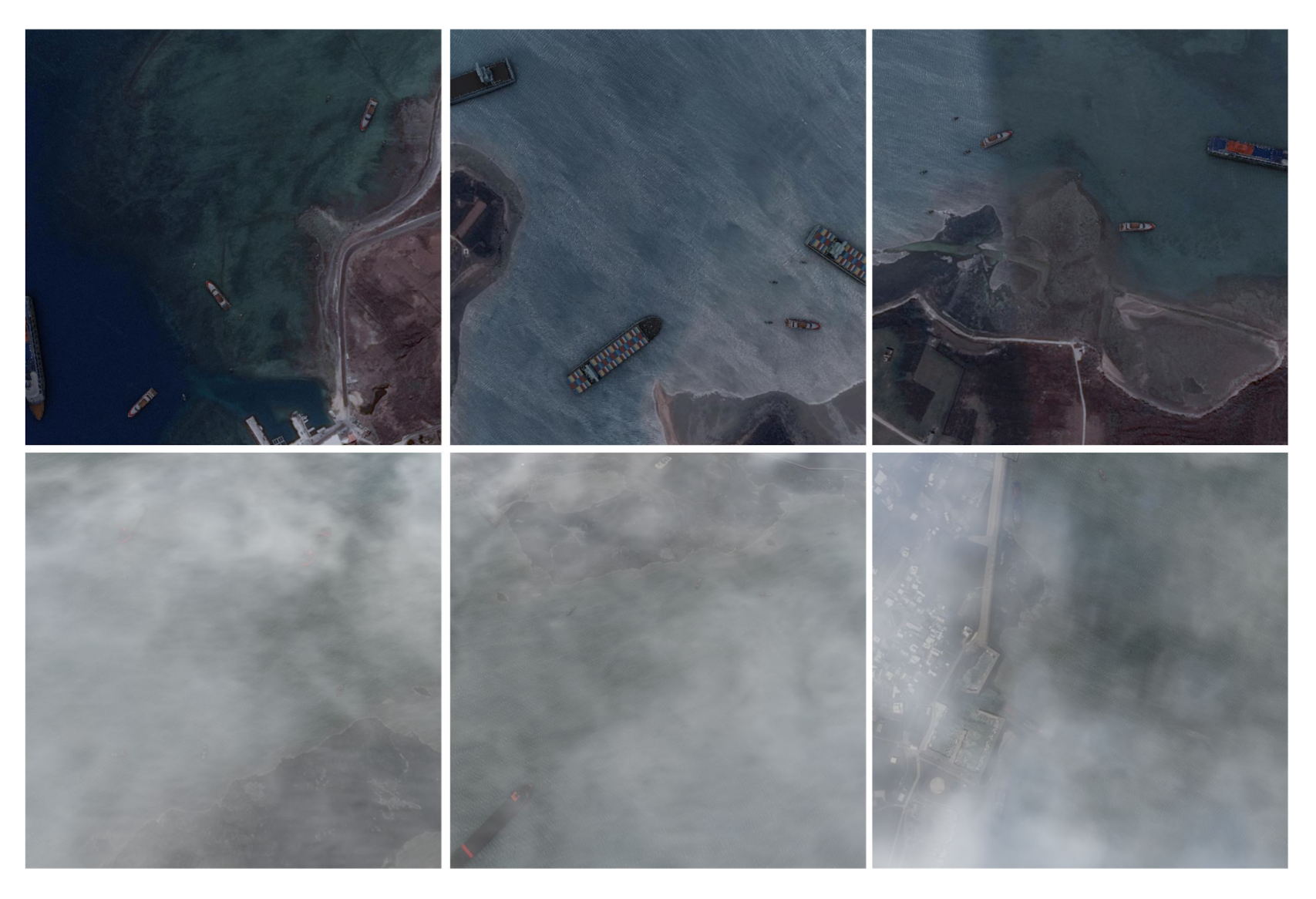
Synthetic remote sensing ship datasets. To verify the superiority of the proposed method in more demanding domain adaption scenarios, we also adopt the synthetic remote sensing image data from the maritime ship detection competition (https://www.datafountain.cn/competitions/275/, date accessed: 9 August 2021) held by the China Computer Federation in the comparison experiments. As shown in the Figure 9, the data are divided into two independent datasets (each of which contains 1500 images) according to different weather conditions, including normal weather (Normal) and cloudy weather (Cloudy).
The network is trained with an Adam optimizer on GTX1080ti GPU with 2 images from different datasets per mini-batch. The input image is resized such that its shorter side has 600 pixels. The backbone network is ResNet-50 [25]. During training, we use a momentum of 0.9 and a weight decay of 0.0005 for optimization. The collection of the two datasets is randomly divided into three parts (training set, validation set, and test set) with a ratio of 6:1:3. We flip each image in horizontal reflections to double the images for data augmentation. The other parameter settings are consistent with those in paper [5]. We use the average precision (AP) calculated in accordance with the PASCAL visual object classes challenge 2007 (VOC2007) [48] as the evaluation metric.
4.2. Experimental Analysis
4.2.1. Evaluation of the Proposed Modules
To verify the superiority of the proposed structures, we conduct several comparisons in Table 1 with a baseline model in which any proposed technology is abandoned. For a fair comparison, any other parameter settings of the baseline model are consistent with the proposed method. In Table 1, MRFI and CDA indicate the multiple receptive field feature integration and the channel domain attention module in image-level adaption, respectively. BR indicates the boundary regression in instance-level adaption.
From Table 1, we can see that the multiple receptive field feature integration can effectively improve the performance of the baseline model on the test set. By combining with the domain attention module, the AP finally achieves a 1.8-point improvement. In addition, the extreme point regression also brings an AP increase of 2.0 points independently. Experimental results show that the instance-level adaption has achieved a higher improvement than the image-level adaption. The reasons may be as follows: (1) for the two datasets, the difference between ship objects is more significant than the background region. (2) The instance-based adaption includes the process of proposal correction. More precise object localization can directly improve the performance of the detection. Finally, by further assembling all these structures together, the proposed model improves the Baseline model by +3.6%, which achieves 89.0% in terms of AP.
4.2.2. Evaluation of the Multiple Receptive Field Feature Integration
The key of multiple receptive field feature integration is the fusion strategy of the feature maps with different receptive fields. Since there are semantic gaps between different feature maps, a simple fusion strategy may not achieve good results. Therefore, we gradually fuse adjacent feature maps, and obtain appropriate fusion weights based on the attention mechanism. As shown in Table 2, we evaluate the performance of the proposed approach with different fusion strategies.
In Table 2, direct means directly splicing the feature maps with different receptive fields along the channel, while gradual means fusing the adjacent feature maps in sequence. The attention-based feature fusion proposed in this paper is indicated by *. Experimental results show that gradual fusion is better than direct fusion, and the weight obtained by the attention-based feature fusion further improves the performance of multiple receptive field feature integration.
4.2.3. Evaluation of the Domain Attention Module
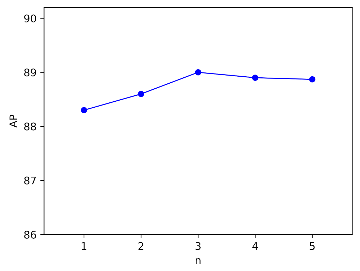
In this section, we will study the influence of the number of SE adapters in the channel domain attention module. As shown in Figure 10, we set a different number of SE adapters (denoted by n) for the channel domain attention module to evaluate their performance. It is worth noting that when , the channel domain attention module degenerates to the standard SE module.
It can be seen from the experimental results that a single SE adapter has the worst performance, since only the channel attention works at this time. When sufficient SE adapters are used ( in our experiment), involving more SE adapters will not bring further performance improvement. This can probably be explained as the following. Although a larger n provides a larger parameter space which helps to sensitively distribute the activation between both of the two domains, more parameters also increase the risk of over-fitting, thus resulting in a performance decrease.
4.2.4. Evaluation of the Boundary Regression Module
The boundary regression module consists of two major components: a convolution head for feature preprocessing, and the extreme point pooling to obtain the features of extreme points for the regression. In this section, we will study the performance of these two components separately.
The experimental results are shown in Table 3, where normal means that the feature obtained from the previous ROI pooling process is used as the pooling input, and conv indicates that the structure shown in Figure 6 is used to process the feature map. For the pooling method, traditional represents the conventional way to divide the proposal into bins for pooling (a feature map of size is obtained after pooling), while the point-based score indicates that the extreme point pooling shown in Figure 7 is performed to obtain four 1024-d vectors for regression. To better evaluate the localization performance, the index of mean intersection-over-union (IoU) is also calculated.
Experimental results show that the conv head boosts both AP and IoU, which means that convolution operation is more suitable for bounding box regression. In addition, although the AP indicator of extreme point pooling is almost the same as the traditional pooling method, we can still see a significant improvement in terms of IoU. This shows that extreme point pooling effectively improves the localization accuracy of the detection.
4.3. Comparison
4.3.1. Domain Adaption on Real Remote Sensing Data
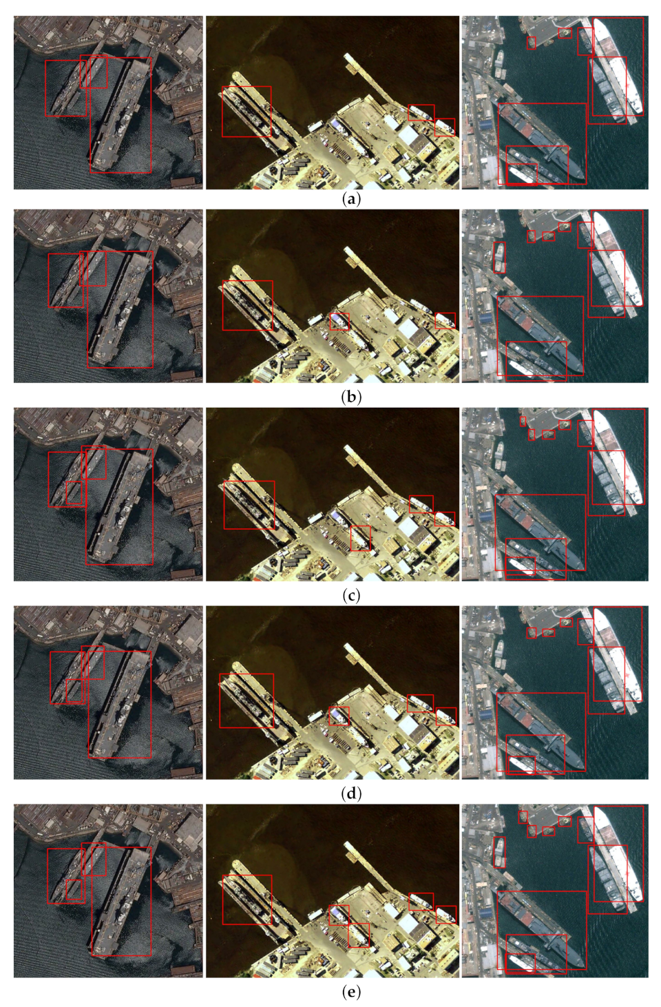
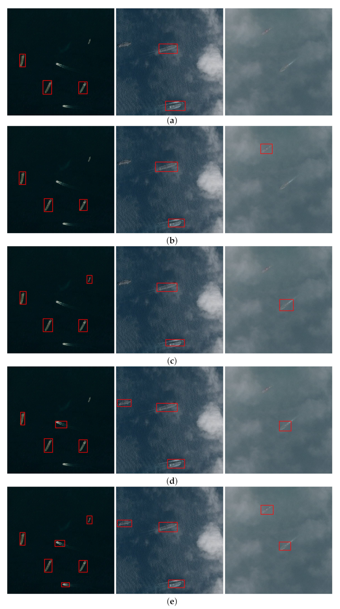
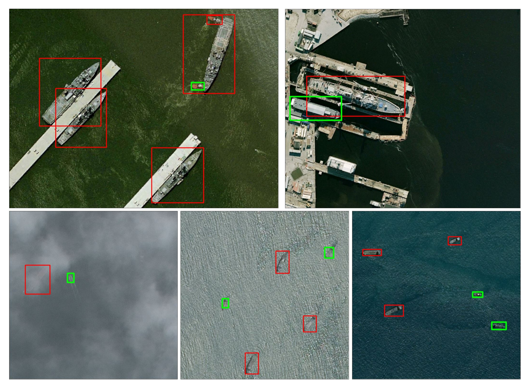
The proposed method is compared with four other representative methods which are Faster R-CNN [5], RetinaNet [8], YOLOv3 [9], and Mask R-CNN [10]. Some examples of the detection results from HRSC2016 and Airbus by different methods are shown in Figure 11 and Figure 12, respectively. Examples of some failed cases are shown in Figure 13.
The three images shown in Figure 11 are all with complex port background interference. It can be seen that the other four methods are all have miss detections to some extent, while the proposed method successfully detects all the ships with various scales. In contrast, images in Figure 12 are all with sea backgrounds. Despite the relatively simple environment compared with the ports, the sea clutter and complicated weather conditions also make it difficult to detect small ships. For example, all the other algorithms fail to detect both of the tiny moving ships in the first image at the same time. Suffering from the bad weather, ships in the other two images are less clear. It can be seen from the results that such blurry ships are easily cause miss detections, while the proposed method successfully detects all these ships. In summary, compared with general detection methods, the proposed method can effectively deal with the domain shift between different datasets, achieving accurate ship detection in both port and sea environments.
4.3.2. Domain Adaption on Synthetic Remote Sensing Data
In addition to adapting between real remote sensing data, synthetic data are also used for the comparison experiments. Specifically, the experiments with synthetic data include HRSC2016 & Normal, HRSC2016 & Cloudy, and Normal & Cloudy. The evaluation results are shown in Table 5.
The experimental results show that, compared with other methods, our proposed method still maintains obvious advantages in all the three adaption scenarios with synthetic data. It should be noted that both the data types and weather conditions between HRSC2016 and Cloudy are different. Therefore, there is a large domain shift between the two datasets, which limits the performance of the detection methods. In contrast, the Normal and Cloudy datasets are both synthetic data. The difference is only in weather conditions, so there is a relatively small domain shift between them. In this case, all methods achieve the best performance compared with the other two sets of experiments.
4.3.3. Unsupervised Domain Adaption
Since it is difficult to acquire and annotate the remote sensing image, we also consider the unsupervised domain adaption scenario and the experimental results are shown in Table 6. We perform the adaption experiments between real remote sensing data and synthetic remote sensing data, respectively. Specifically, we use the HRSC2016 dataset as the source domain for which images and their bounding box annotations are provided, and the Airbus dataset as the target domain for which only unlabeled images are available. All images from the source domain are used for training, while 30% of the images from the target domain are reserved to evaluate the performance of the trained model. In the experiment on synthetic data, the Normal dataset is used as the source domain, while the Cloudy dataset is used as the target domain.
The proposed method is compared with three other representative domain adaption methods which are method [20], method [21] and method [22]. We also present the evaluation results of the baseline model proposed in Section 4.2.1 to verify the effectiveness of the domain adaptation technology. As shown in Table 6, the proposed method outperforms all the other relevant methods on both of the two unsupervised domain scenarios.
5. Conclusions
In this paper, we propose a novel CNN-based domain adaptive ship detection method for cross-domain ship detection in optical remote sensing images. The proposed method alleviates the performance drop caused by domain shift via both image-level adaption and instance-level adaption. In image-level adaption, we utilize multiple receptive field feature integration and channel domain adaption to improve the feature representation ability of the network between the two domains. In instance-level adaption, a novel boundary regression module is proposed to correct the region proposals with the corresponding effective extreme point features. During training, the network learns suitable feature representations for both of the two domains with the help of the domain classifiers, thereby improving the generalization ability of the trained model. In addition, the proposed method is also suitable for the unsupervised domain adaption scenario. Detailed ablation studies and the comparison results with other algorithms verify the superiority of our method.
Author Contributions
Conceptualization, L.L.; methodology, L.L., Z.Z. and B.W.; software, L.L.; validation, L.L., Z.Z., B.W. and L.M.; formal analysis, L.L.; investigation, Z.A. and X.X.; resources, L.M.; data curation, L.L.; writing—original draft preparation, L.L.; writing—review and editing, L.L. and Z.Z.; visualization, Z.A. and X.X.; supervision, L.M.; project administration, L.L. All authors have read and agreed to the published version of the manuscript.
Funding
This research received no external funding.
Institutional Review Board Statement
Not applicable.
Informed Consent Statement
Not applicable.
Data Availability Statement
Not applicable.
Conflicts of Interest
The authors declare no conflict of interest.
References
- Girshick, R. Fast r-cnn. In Proceedings of the IEEE International Conference on Computer Vision, Santiago, Chile, 7–13 December 2015; pp. 1440–1448. [Google Scholar]
- Redmon, J.; Divvala, S.; Girshick, R.; Farhadi, A. You only look once: Unified, real-time object detection. In Proceedings of the IEEE Conference on Computer Vision and Pattern Recognition, Las Vegas, NV, USA, 27–30 June 2016; pp. 779–788. [Google Scholar]
- Liu, W.; Anguelov, D.; Erhan, D.; Szegedy, C.; Reed, S.; Fu, C.Y.; Berg, A.C. Ssd: Single shot multibox detector. In European Conference on Computer Vision; Springer: Berlin, Germany, 2016; pp. 21–37. [Google Scholar]
- Dai, J.; Li, Y.; He, K.; Sun, J. R-fcn: Object detection via region-based fully convolutional networks. In Proceedings of the Advances in Neural Information Processing Systems, Barcelona, Spain, 5–10 December 2016; pp. 379–387. [Google Scholar]
- Ren, S.; He, K.; Girshick, R.; Sun, J. Faster R-CNN: Towards Real-Time Object Detection with Region Proposal Networks. IEEE Trans. Pattern Anal. Mach. Intell. 2017, 39, 1137. [Google Scholar] [CrossRef] [PubMed] [Green Version]
- Redmon, J.; Farhadi, A. YOLO9000: Better, faster, stronger. In Proceedings of the IEEE Conference on Computer Vision and Pattern Recognition, Honolulu, HI, USA, 21–26 July 2017; pp. 7263–7271. [Google Scholar]
- Lin, T.Y.; Dollár, P.; Girshick, R.; He, K.; Hariharan, B.; Belongie, S. Feature pyramid networks for object detection. In Proceedings of the IEEE Conference on Computer Vision and Pattern Recognition, Honolulu, HI, USA, 21–26 July 2017; pp. 2117–2125. [Google Scholar]
- Lin, T.Y.; Goyal, P.; Girshick, R.; He, K.; Dollár, P. Focal loss for dense object detection. In Proceedings of the IEEE International Conference on Computer Vision, Venice, Italy, 22–29 October 2017; pp. 2980–2988. [Google Scholar]
- Redmon, J.; Farhadi, A. Yolov3: An incremental improvement. arXiv 2018, arXiv:1804.02767. [Google Scholar]
- He, K.; Gkioxari, G.; Dollár, P.; Girshick, R. Mask r-cnn. In Proceedings of the IEEE International Conference on Computer Vision, Venice, Italy, 22–29 October 2017; pp. 2961–2969. [Google Scholar]
- Li, Q.; Mou, L.; Liu, Q.; Wang, Y.; Zhu, X.X. HSF-Net: Multiscale deep feature embedding for ship detection in optical remote sensing imagery. IEEE Trans. Geosci. Remote Sens. 2018, 56, 7147–7161. [Google Scholar] [CrossRef]
- Nie, S.; Jiang, Z.; Zhang, H.; Cai, B.; Yao, Y. Inshore ship detection based on mask R-CNN. In Proceedings of the IGARSS 2018–2018 IEEE International Geoscience and Remote Sensing Symposium, Valencia, Spain, 22–27 July 2018; pp. 693–696. [Google Scholar]
- Liu, W.; Ma, L.; Chen, H. Arbitrary-oriented ship detection framework in optical remote-sensing images. IEEE Geosci. Remote Sens. Lett. 2018, 15, 937–941. [Google Scholar] [CrossRef]
- Yang, X.; Sun, H.; Fu, K.; Yang, J.; Sun, X.; Yan, M.; Guo, Z. Automatic ship detection in remote sensing images from google earth of complex scenes based on multiscale rotation dense feature pyramid networks. Remote Sens. 2018, 10, 132. [Google Scholar] [CrossRef] [Green Version]
- Zhang, S.; Wu, R.; Xu, K.; Wang, J.; Sun, W. R-CNN-based ship detection from high resolution remote sensing imagery. Remote Sens. 2019, 11, 631. [Google Scholar] [CrossRef] [Green Version]
- Li, L.; Zhou, Z.; Wang, B.; Miao, L.; Zong, H. A Novel CNN-Based Method for Accurate Ship Detection in HR Optical Remote Sensing Images via Rotated Bounding Box. IEEE Trans. Geosci. Remote Sens. 2020, 59, 686–699. [Google Scholar] [CrossRef]
- Ming, Q.; Zhou, Z.; Miao, L.; Zhang, H.; Li, L. Dynamic Anchor Learning for Arbitrary-Oriented Object Detection. In Proceedings of the AAAI Conference on Artificial Intelligence, Palo Alto, CA, USA, 2–9 February 2021. [Google Scholar]
- Chen, L.; Shi, W.; Deng, D. Improved YOLOv3 Based on Attention Mechanism for Fast and Accurate Ship Detection in Optical Remote Sensing Images. Remote Sens. 2021, 13, 660. [Google Scholar] [CrossRef]
- Gopalan, R.; Li, R.; Chellappa, R. Domain adaptation for object recognition: An unsupervised approach. In Proceedings of the 2011 International Conference on Computer Vision, Barcelona, Spain, 6–13 November 2011; pp. 999–1006. [Google Scholar]
- Chen, Y.; Li, W.; Sakaridis, C.; Dai, D.; Van Gool, L. Domain adaptive faster r-cnn for object detection in the wild. In Proceedings of the IEEE Conference on Computer Vision and Pattern Recognition, Salt Lake City, UT, USA, 18–23 June 2018; pp. 3339–3348. [Google Scholar]
- Saito, K.; Ushiku, Y.; Harada, T.; Saenko, K. Strong-weak distribution alignment for adaptive object detection. In Proceedings of the IEEE Conference on Computer Vision and Pattern Recognition, Long Beach, CA, USA, 16–17 June 2019; pp. 6956–6965. [Google Scholar]
- Xie, R.; Yu, F.; Wang, J.; Wang, Y.; Zhang, L. Multi-Level Domain Adaptive Learning for Cross-Domain Detection. In Proceedings of the IEEE International Conference on Computer Vision Workshops, Seoul, Korea, 27–28 October 2019. [Google Scholar]
- Hu, J.; Shen, L.; Sun, G. Squeeze-and-excitation networks. In Proceedings of the IEEE Conference on Computer Vision and Pattern Recognition, Salt Lake City, UT, USA, 18–23 June 2018; pp. 7132–7141. [Google Scholar]
- Krizhevsky, A.; Sutskever, I.; Hinton, G.E. Imagenet classification with deep convolutional neural networks. Adv. Neural Inf. Process. Syst. 2012, 25, 1097–1105. [Google Scholar] [CrossRef]
- He, K.; Zhang, X.; Ren, S.; Sun, J. Deep residual learning for image recognition. In Proceedings of the IEEE Conference on Computer Vision and Pattern Recognition, Las Vegas, NV, USA, 27–30 June 2016; pp. 770–778. [Google Scholar]
- Huang, G.; Liu, Z.; Van Der Maaten, L.; Weinberger, K.Q. Densely connected convolutional networks. In Proceedings of the IEEE Conference on Computer Vision and Pattern Recognition, Honolulu, HI, USA, 21–26 July 2017; pp. 4700–4708. [Google Scholar]
- Long, J.; Shelhamer, E.; Darrell, T. Fully convolutional networks for semantic segmentation. In Proceedings of the IEEE Conference on Computer Vision and Pattern Recognition, Boston, MA, USA, 7–12 June 2015; pp. 3431–3440. [Google Scholar]
- Badrinarayanan, V.; Kendall, A.; Cipolla, R. Segnet: A deep convolutional encoder-decoder architecture for image segmentation. IEEE Trans. Pattern Anal. Mach. Intell. 2017, 39, 2481–2495. [Google Scholar] [CrossRef] [PubMed]
- Chen, L.C.; Papandreou, G.; Kokkinos, I.; Murphy, K.; Yuille, A.L. Deeplab: Semantic image segmentation with deep convolutional nets, atrous convolution, and fully connected crfs. IEEE Trans. Pattern Anal. Mach. Intell. 2017, 40, 834–848. [Google Scholar] [CrossRef] [PubMed]
- Lei, L.; Su, Y. An inshore ship detection method based on contour matching. Remote Sens. Technol. Appl. 2007, 22, 622–627. [Google Scholar]
- Lin, J.; Yang, X.; Xiao, S.; Yu, Y.; Jia, C. A line segment based inshore ship detection method. In Future Control and Automation; Springer: Berlin, Germany, 2012; pp. 261–269. [Google Scholar]
- Zhu, C.; Zhou, H.; Wang, R.; Guo, J. A novel hierarchical method of ship detection from spaceborne optical image based on shape and texture features. IEEE Trans. Geosci. Remote Sens. 2010, 48, 3446–3456. [Google Scholar] [CrossRef]
- Li, S.; Zhou, Z.; Wang, B.; Wu, F. A novel inshore ship detection via ship head classification and body boundary determination. IEEE Geosci. Remote Sens. Lett. 2016, 13, 1920–1924. [Google Scholar] [CrossRef]
- Liu, G.; Zhang, Y.; Zheng, X.; Sun, X.; Fu, K.; Wang, H. A new method on inshore ship detection in high-resolution satellite images using shape and context information. IEEE Geosci. Remote Sens. Lett. 2013, 11, 617–621. [Google Scholar] [CrossRef]
- Yang, F.; Xu, Q.; Li, B. Ship detection from optical satellite images based on saliency segmentation and structure-LBP feature. IEEE Geosci. Remote Sens. Lett. 2017, 14, 602–606. [Google Scholar] [CrossRef]
- Ganin, Y.; Lempitsky, V. Unsupervised domain adaptation by backpropagation. In Proceedings of the International Conference on Machine Learning, PMLR, Lille, France, 7–9 July 2015; pp. 1180–1189. [Google Scholar]
- Ganin, Y.; Ustinova, E.; Ajakan, H.; Germain, P.; Larochelle, H.; Laviolette, F.; Marchand, M.; Lempitsky, V. Domain-adversarial training of neural networks. J. Mach. Learn. Res. 2016, 17, 2030–2096. [Google Scholar]
- Tzeng, E.; Hoffman, J.; Saenko, K.; Darrell, T. Adversarial discriminative domain adaptation. In Proceedings of the IEEE Conference on Computer Vision and Pattern Recognition, Honolulu, HI, USA, 21–26 July 2017; pp. 7167–7176. [Google Scholar]
- Tsai, Y.H.; Hung, W.C.; Schulter, S.; Sohn, K.; Yang, M.H.; Chandraker, M. Learning to adapt structured output space for semantic segmentation. In Proceedings of the IEEE Conference on Computer Vision and Pattern Recognition, Salt Lake City, UT, USA, 18–23 June 2018; pp. 7472–7481. [Google Scholar]
- Goodfellow, I.J.; Pouget-Abadie, J.; Mirza, M.; Xu, B.; Warde-Farley, D.; Ozair, S.; Courville, A.; Bengio, Y. Generative adversarial nets. In Proceedings of the 27th International Conference on Neural Information Processing Systems-Volume 2, Montreal, QC, Canada, 8–13 December 2014; pp. 2672–2680. [Google Scholar]
- Peng, C.; Zhang, X.; Yu, G.; Luo, G.; Sun, J. Large kernel matters–improve semantic segmentation by global convolutional network. In Proceedings of the IEEE Conference on Computer Vision and Pattern Recognition, Honolulu, HI, USA, 21–26 July 2017; pp. 4353–4361. [Google Scholar]
- Simonyan, K.; Zisserman, A. Very deep convolutional networks for large-scale image recognition. arXiv 2014, arXiv:1409.1556. [Google Scholar]
- Yu, F.; Koltun, V.; Funkhouser, T. Dilated residual networks. In Proceedings of the IEEE Conference on Computer Vision and Pattern Recognition, Honolulu, HI, USA, 21–26 July 2017; pp. 472–480. [Google Scholar]
- Li, Z.; Peng, C.; Yu, G.; Zhang, X.; Deng, Y.; Sun, J. Detnet: A backbone network for object detection. arXiv 2018, arXiv:1804.06215. [Google Scholar]
- Dai, Y.; Gieseke, F.; Oehmcke, S.; Wu, Y.; Barnard, K. Attentional feature fusion. In Proceedings of the IEEE/CVF Winter Conference on Applications of Computer Vision, Waikola, HI, USA, 5–9 January 2021; pp. 3560–3569. [Google Scholar]
- Wang, X.; Cai, Z.; Gao, D.; Vasconcelos, N. Towards universal object detection by domain attention. In Proceedings of the IEEE/CVF Conference on Computer Vision and Pattern Recognition, Long Beach, CA, USA, 15–21 June 2019; pp. 7289–7298. [Google Scholar]
- Liu, Z.; Wang, H.; Weng, L.; Yang, Y. Ship rotated bounding box space for ship extraction from high-resolution optical satellite images with complex backgrounds. IEEE Geosci. Remote Sens. Lett. 2016, 13, 1074–1078. [Google Scholar] [CrossRef]
- Everingham, M.; Van Gool, L.; Williams, C.K.; Winn, J.; Zisserman, A. The pascal visual object classes (voc) challenge. Int. J. Comput. Vis. 2010, 88, 303–338. [Google Scholar] [CrossRef] [Green Version]
Figure 1.
The pipeline of the proposed method.

Figure 2.
Illustration of the multiple receptive field feature integration. A and B represent two different types of residual modules, respectively, while Att represents the attention-based feature fusion.
Figure 2.
Illustration of the multiple receptive field feature integration. A and B represent two different types of residual modules, respectively, while Att represents the attention-based feature fusion.

Figure 3.
Illustration of the residual blocks in multiple receptive field feature integration. (a) Structure A with convolutional mapping. (b) Structure B with identity mapping.
Figure 3.
Illustration of the residual blocks in multiple receptive field feature integration. (a) Structure A with convolutional mapping. (b) Structure B with identity mapping.

Figure 4.
Illustration of the attention-based feature fusion.

Figure 5.
Structure of the channel domain attention module.

Figure 6.
Structure of the boundary regression module.

Figure 7.
Illustration of the extreme point pooling.

Figure 8.
Typical images in HRSC2016 dataset (the first row) and Airbus dataset (the second row).

Figure 9.
Typical images in Normal dataset (the first row) and Cloudy dataset (the second row).

Figure 10.
AP versus the number of SE adapters.

Figure 11.
Comparison of the ship-detection results by different methods on the HRSC2016 dataset. (a) Faster R-CNN [5]. (b) RetinaNet [8]. (c) YOLOv3 [9]. (d) Mask R-CNN [10]. (e) Our method.

Figure 12.
Comparison of the ship-detection results by different methods on the Airbus dataset. (a) Faster R-CNN [5]. (b) RetinaNet [8]. (c)YOLOv3 [9]. (d) Mask R-CNN [10]. (e) Our method.

Figure 13.
Some failed cases of the proposed method. The missed detections are marked by green boxes.
Figure 13.
Some failed cases of the proposed method. The missed detections are marked by green boxes.


Table 1.
Quantitative evaluation of the proposed modules.
| MRFI | CDA | BR | AP | |
|---|---|---|---|---|
| Baseline | 85.4% | |||
| Ours | √ | 86.5% | ||
| √ | √ | 87.2% | ||
| √ | 87.4% | |||
| √ | √ | √ | 89.0% |
Table 2.
Quantitative evaluation of the multiple receptive field feature integration.
| Direct | Gradual | Gradual * | |
|---|---|---|---|
| AP | 88.1% | 88.6% | 89.0% |
* means the attention-based feature fusion proposed in this paper.
Table 3.
Quantitative evaluation of the boundary regression module.
| Pooling Head | Pooling Meathod | AP | IoU |
|---|---|---|---|
| normal | traditional | 88.5% | 0.798 |
| conv | traditional | 88.9% | 0.805 |
| conv | point-based | 89.0% | 0.819 |
Table 4.
Quantitative comparison results on real remote sensing data.
| Faster R-CNN | RetinaNet | YOLOv3 | Mask R-CNN | Our Method | |
|---|---|---|---|---|---|
| AP | |||||
| Recall | |||||
| Precision | |||||
| Running Time | 71 ms | 73 ms | 55 ms | 144 ms | 83 ms |
The best results are marked in bold.
Table 5.
Quantitative comparison results on synthetic remote sensing data.
| Faster R-CNN | RetinaNet | YOLOv3 | Mask R-CNN | Our method | |
|---|---|---|---|---|---|
| HRSC2016 & Normal | 83.0% | 86.4% | 86.9% | 87.7% | 88.7% |
| HRSC2016 & Cloudy | 82.4% | 85.9% | 86.3% | 87.4% | 88.5% |
| Normal & Cloudy | 83.2% | 86.5% | 87.1% | 88.0% | 88.8% |
The best results are marked in bold.
Publisher’s Note: MDPI stays neutral with regard to jurisdictional claims in published maps and institutional affiliations. |
© 2021 by the authors. Licensee MDPI, Basel, Switzerland. This article is an open access article distributed under the terms and conditions of the Creative Commons Attribution (CC BY) license (https://creativecommons.org/licenses/by/4.0/).
Share and Cite
MDPI and ACS Style
Li, L.; Zhou, Z.; Wang, B.; Miao, L.; An, Z.; Xiao, X. Domain Adaptive Ship Detection in Optical Remote Sensing Images. Remote Sens. 2021, 13, 3168. https://0-doi-org.brum.beds.ac.uk/10.3390/rs13163168
AMA Style
Li L, Zhou Z, Wang B, Miao L, An Z, Xiao X. Domain Adaptive Ship Detection in Optical Remote Sensing Images. Remote Sensing. 2021; 13(16):3168. https://0-doi-org.brum.beds.ac.uk/10.3390/rs13163168
Chicago/Turabian StyleLi, Linhao, Zhiqiang Zhou, Bo Wang, Lingjuan Miao, Zhe An, and Xiaowu Xiao. 2021. "Domain Adaptive Ship Detection in Optical Remote Sensing Images" Remote Sensing 13, no. 16: 3168. https://0-doi-org.brum.beds.ac.uk/10.3390/rs13163168
Note that from the first issue of 2016, this journal uses article numbers instead of page numbers. See further details here.