
Self-Attention-Based Conditional Variational Auto-Encoder Generative Adversarial Networks for Hyperspectral Classification

Abstract
:1. Introduction
2. Related Work
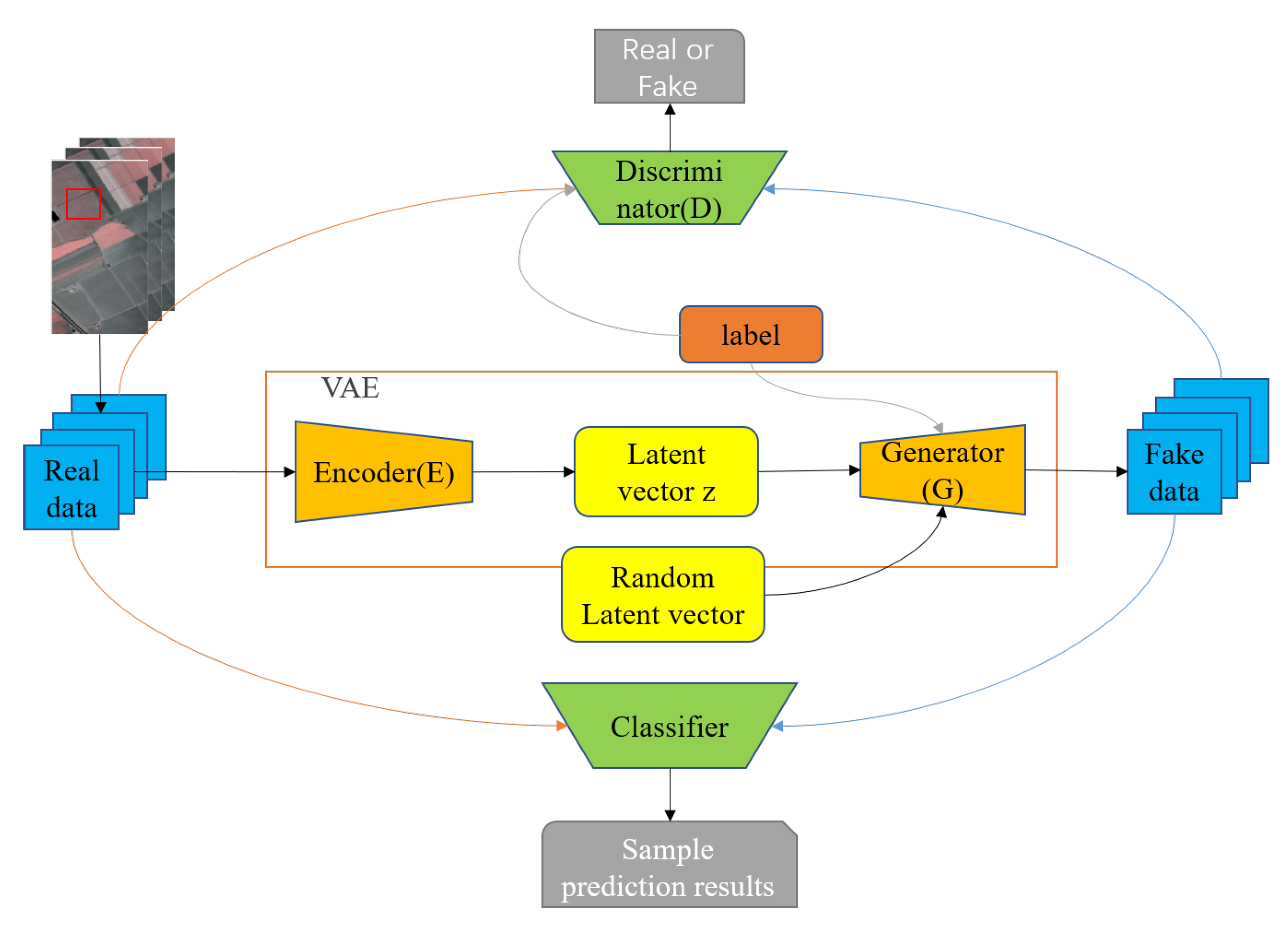
2.1. Conditional Variational Auto-Encoder Generative Adversarial Networks
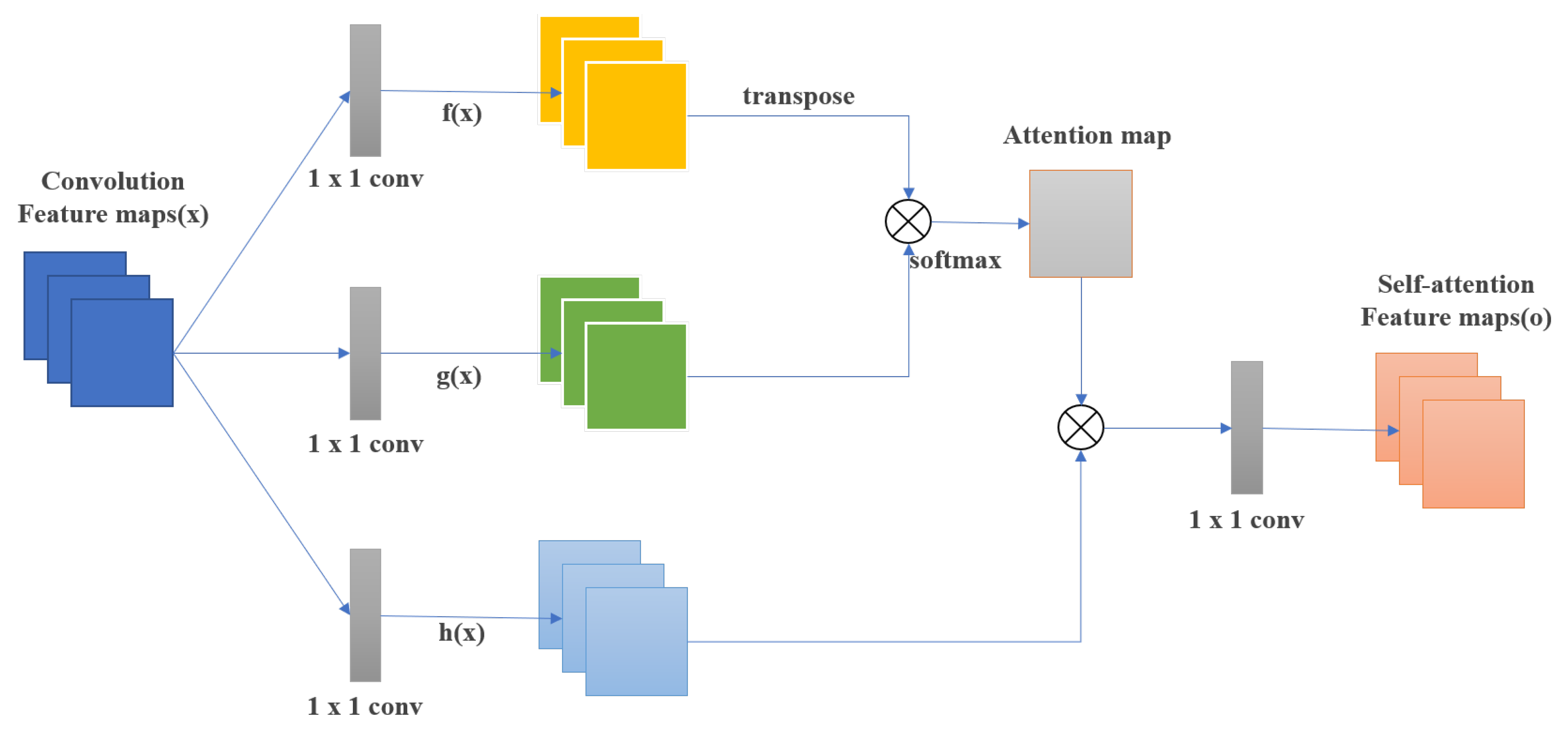
2.2. Self-Attention
3. Methodology
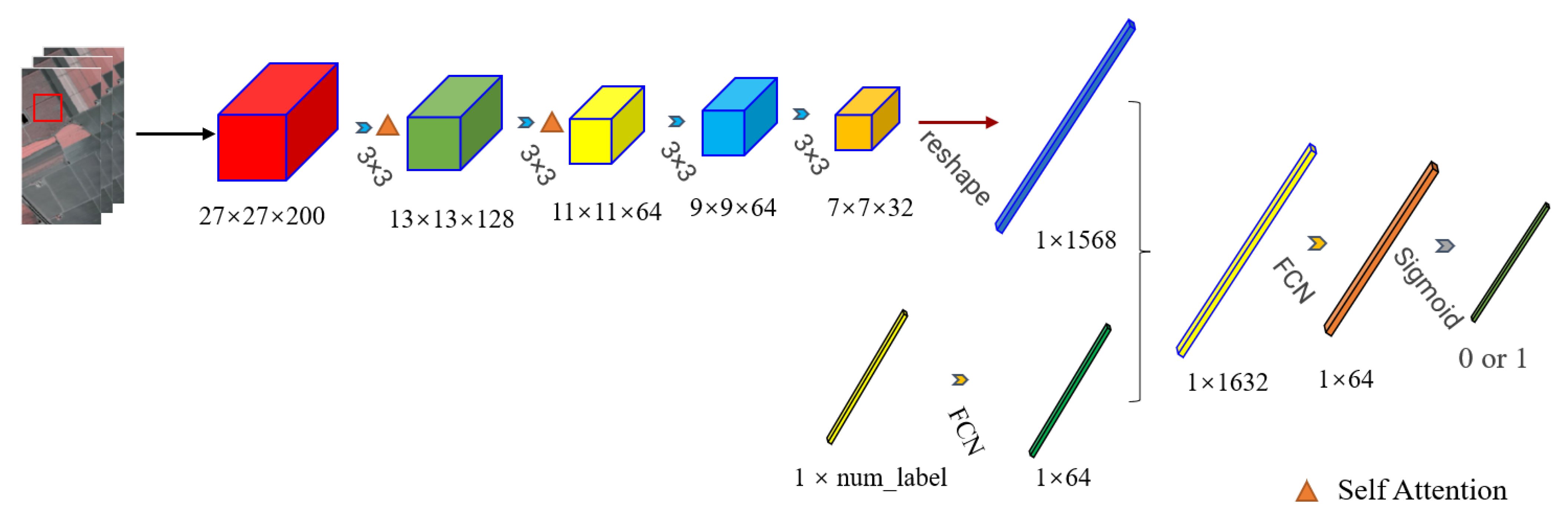
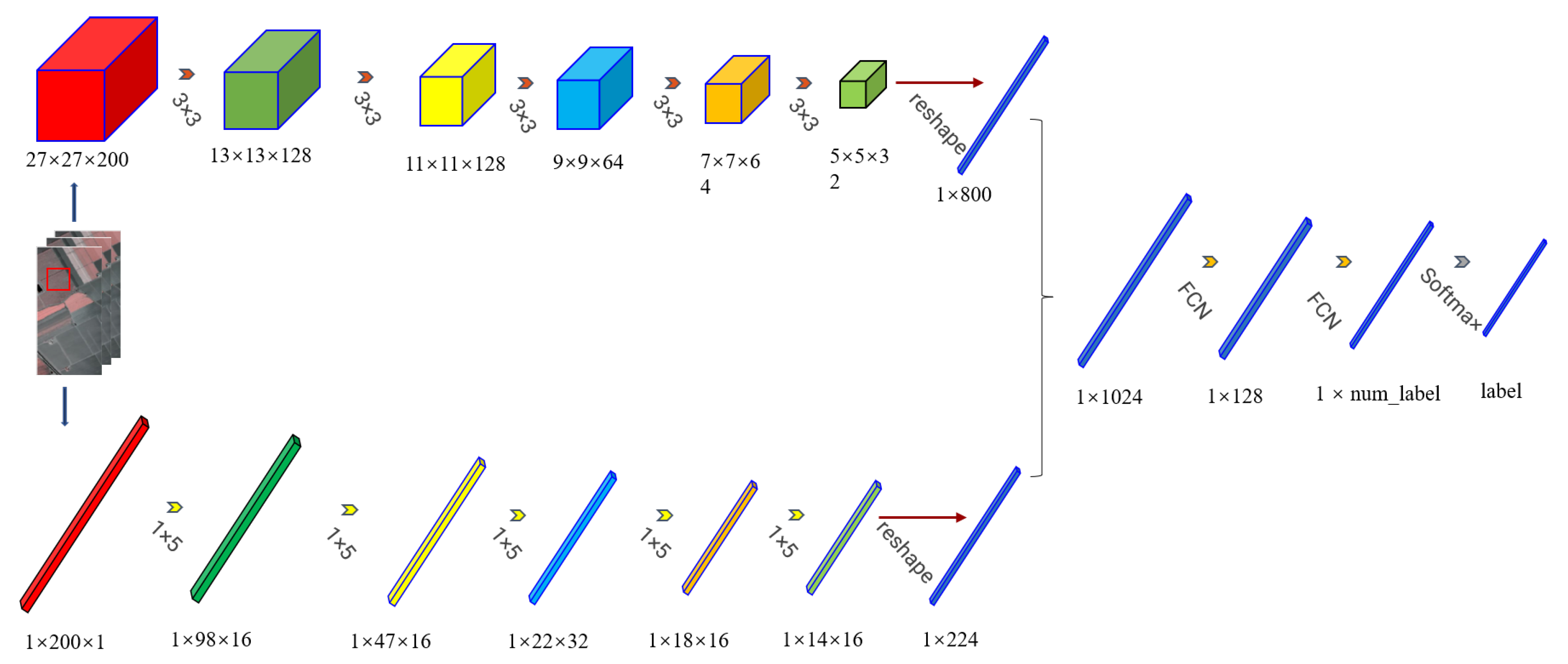
3.1. Discriminator
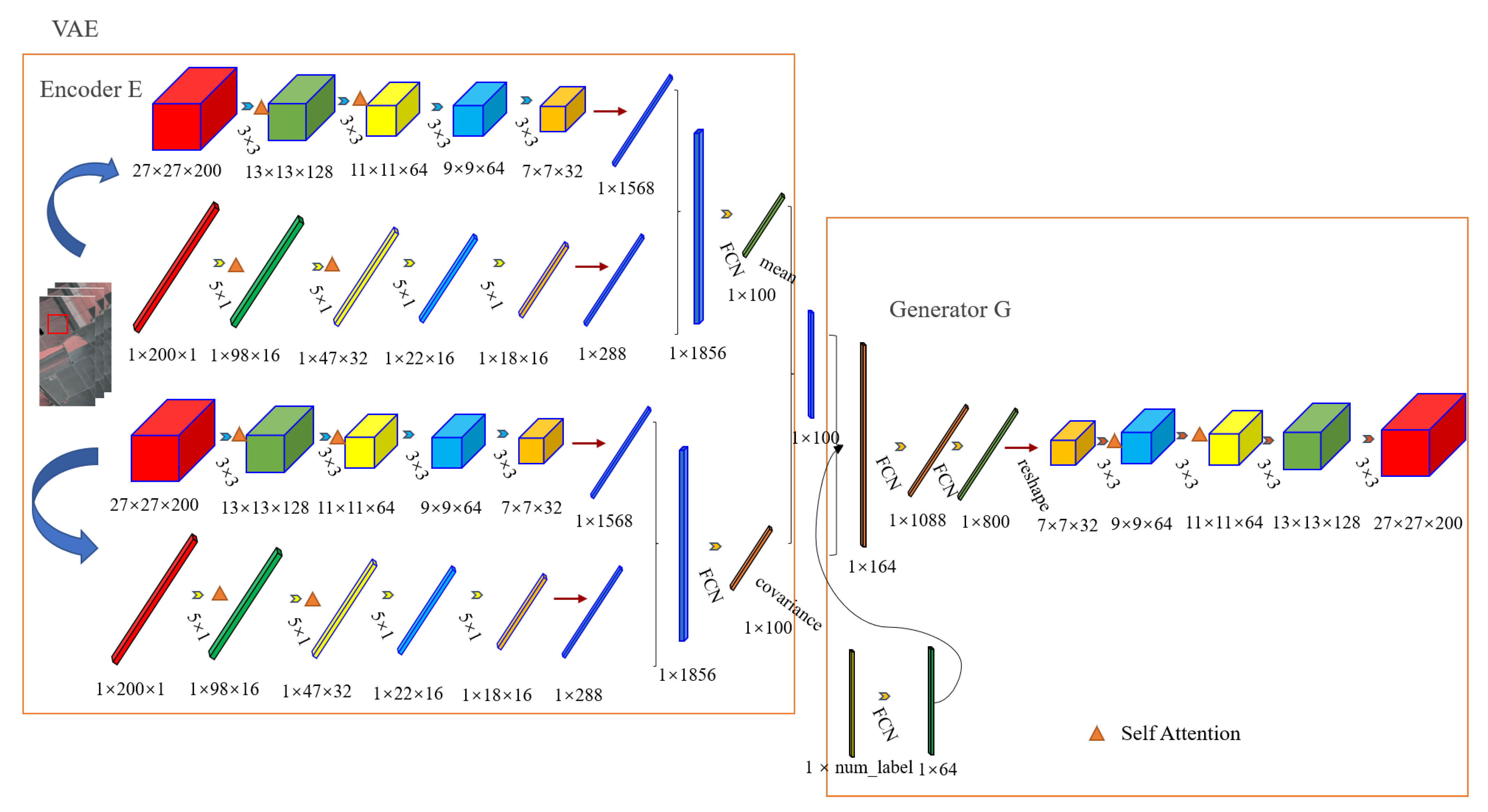
3.2. Variational Auto-Encoder
3.3. Classifier
| Algorithm 1: Optimization procedure of SACVAEGAN. |
| Input: the training samples = and test samples from C classes, the onehot lables of training samples, batch size n, the number of training epochs E, noise dimension d, the updating times k of the discriminator 1 Initialize all the weight matrices and biases 2 while every epoch do 3 sample d dimensional noises = ; 4 generate n latent vectors z = by Encoder E 5 generate n virtual samples through the generator according to the latent vector z; 6 generate n virtual samples through the generator according to the latent vector ; 7 for k steps do 8 updating parameters of the D by minimizing L 9 end 10 updating parameters of the VAE by minimizing L 11 updating parameters of C by minimizing L 12 end Output: the labels of the test samples classified by the trained sample classifier in SACVAEGAN |
4. Experiments
4.1. Hyperspectral Data Sets
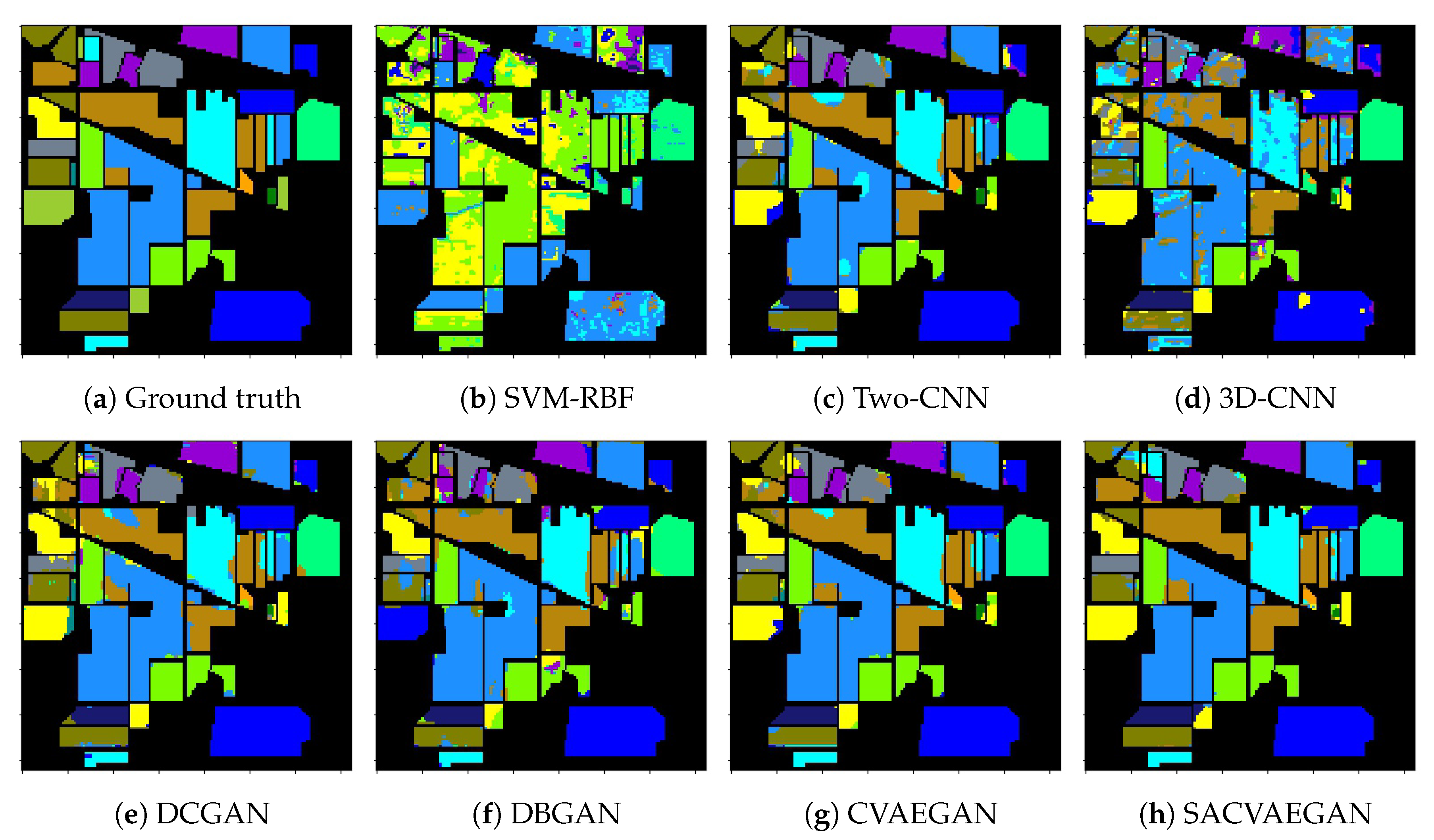
4.1.1. Indian Pines
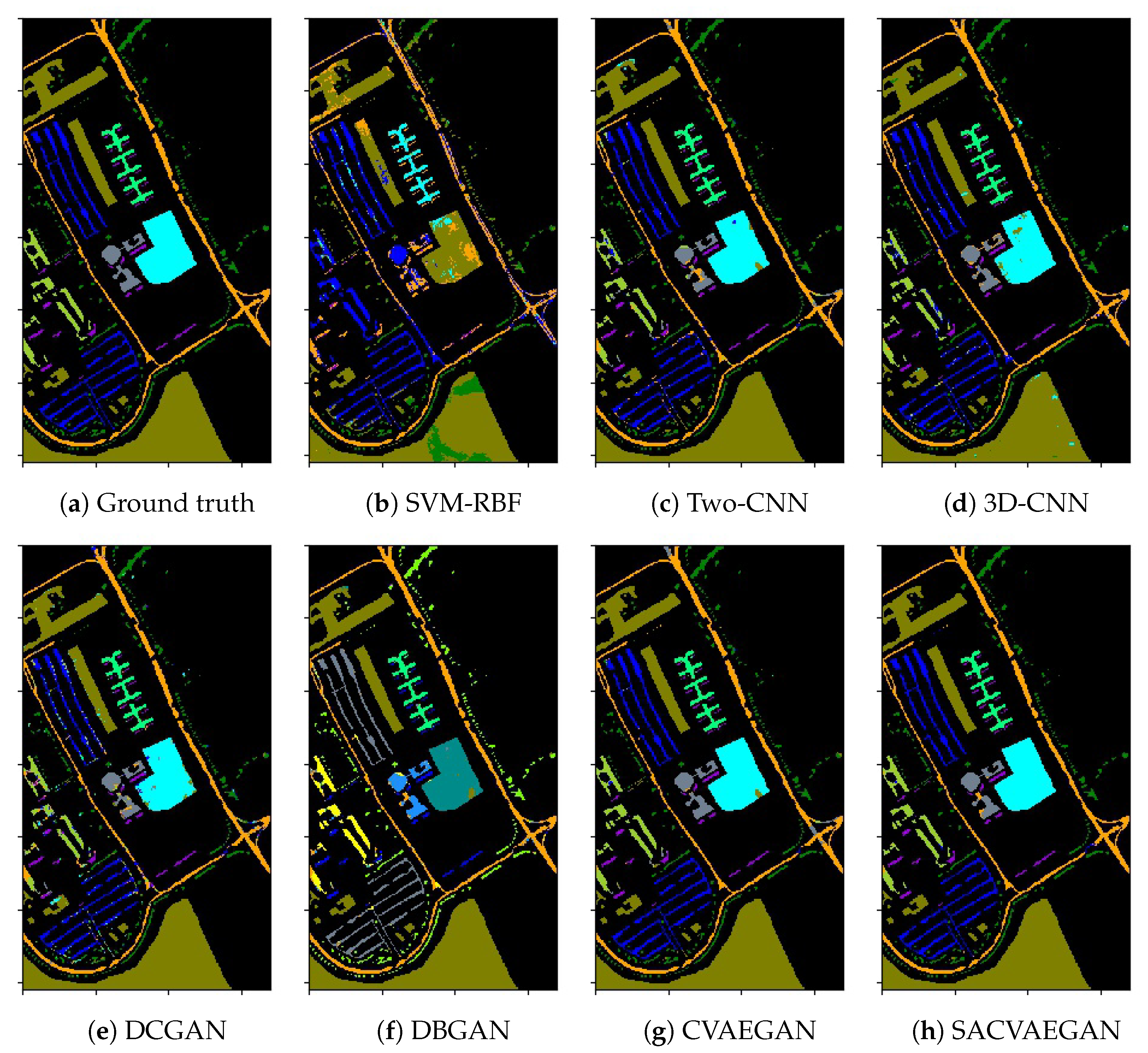
4.1.2. Paviau
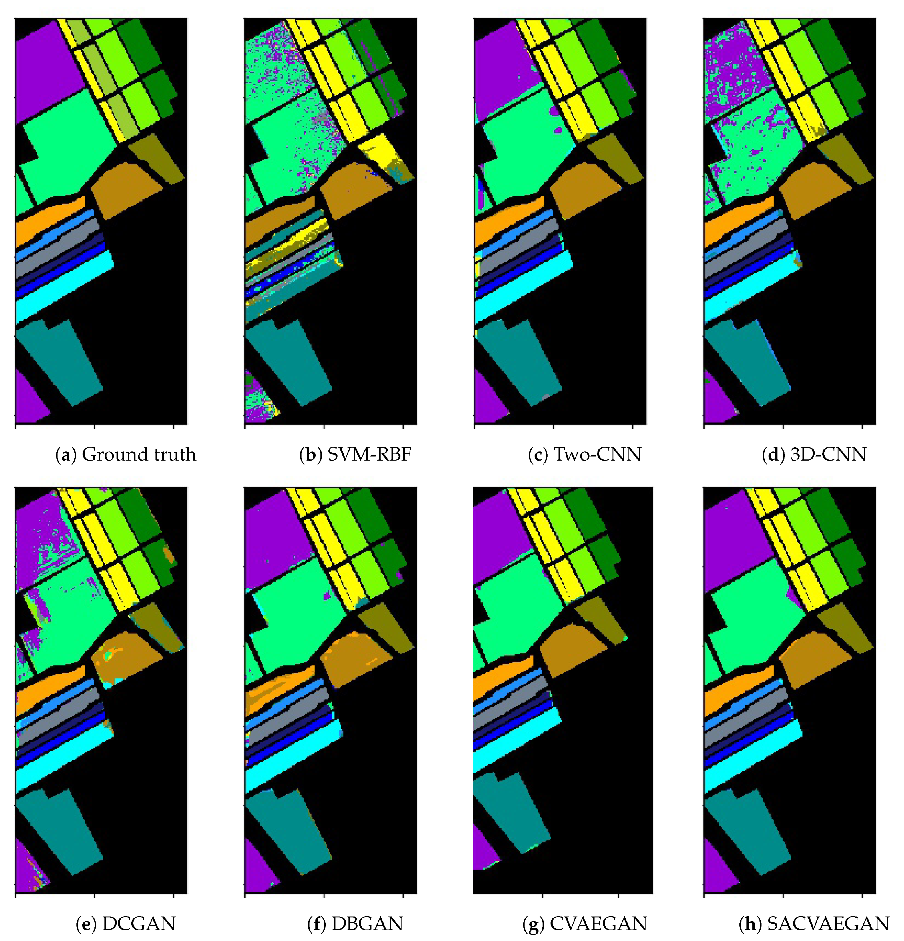
4.1.3. Salinas
4.2. Parameter Analysis
4.2.1. Analysis of the Size of Patches
4.2.2. Analysis of the Network Regularization Method
4.2.3. Analysis of the and in the Classifier Loss Function
4.3. Classification Results
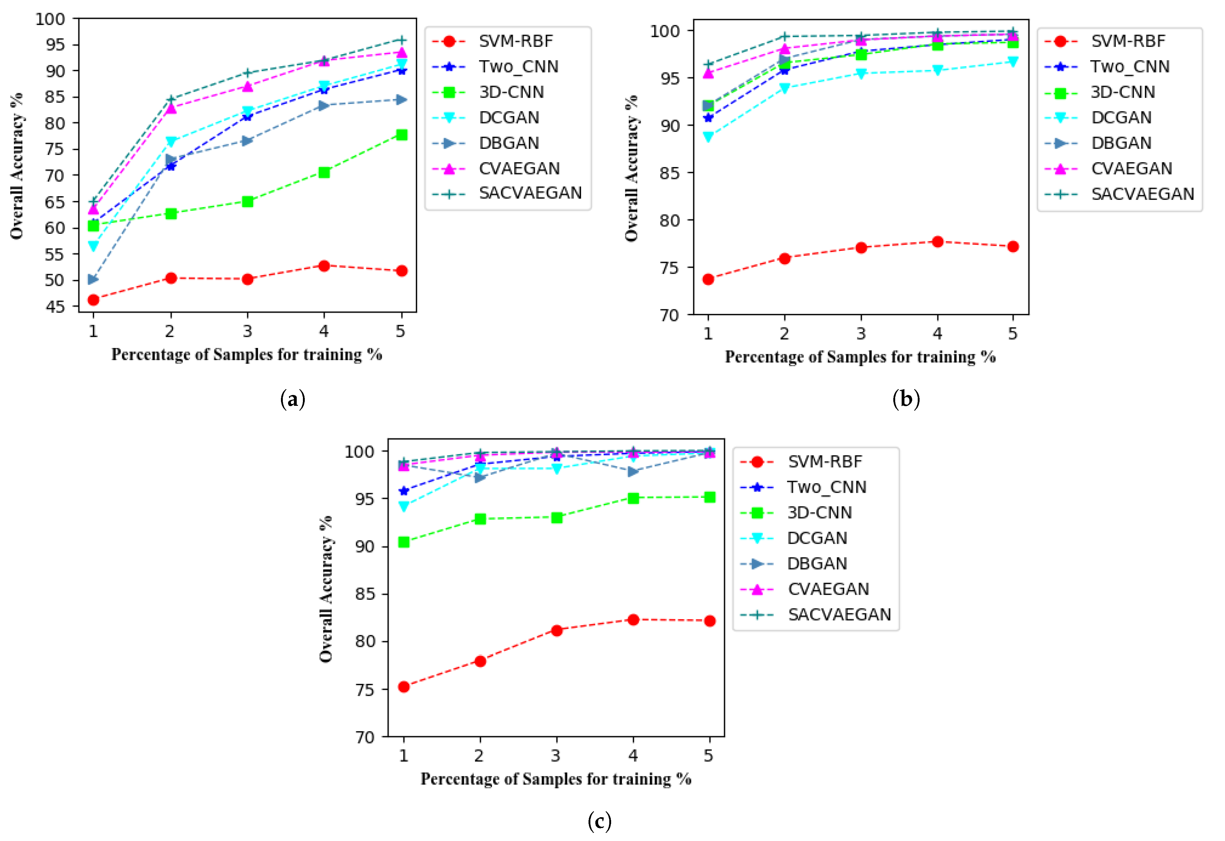
4.4. Analysis of the Size of the Training Set
4.5. Investigation on the Run Time
5. Discussion
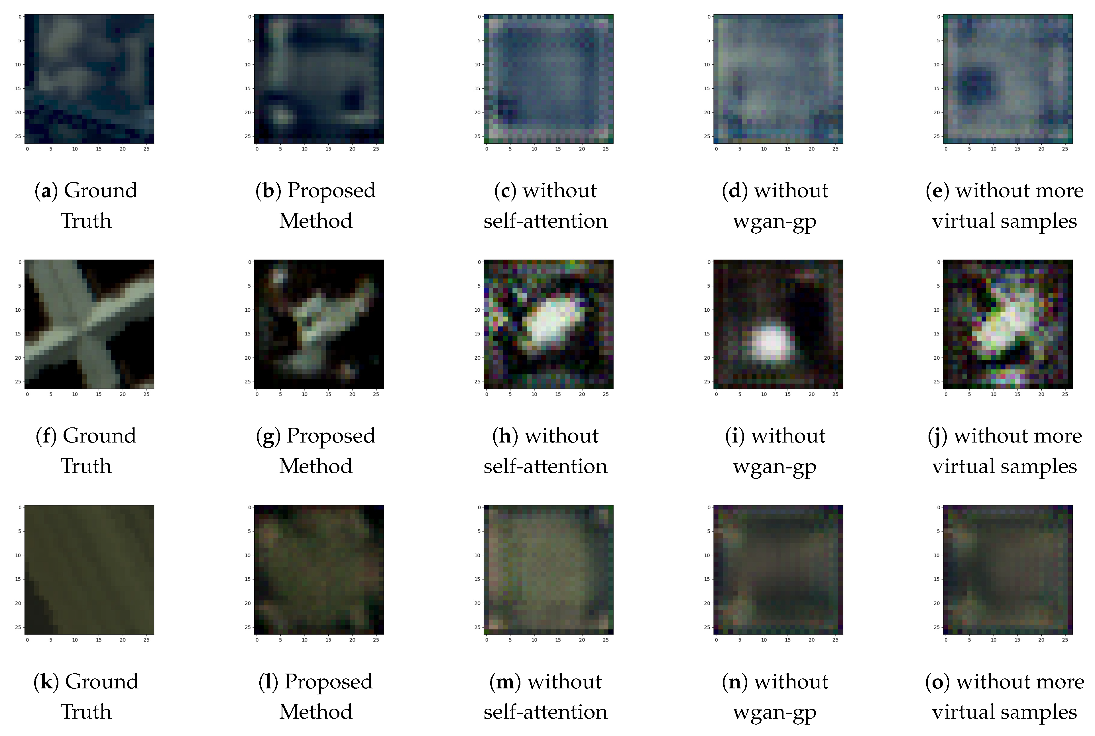
5.1. Spatial Feature Analysis
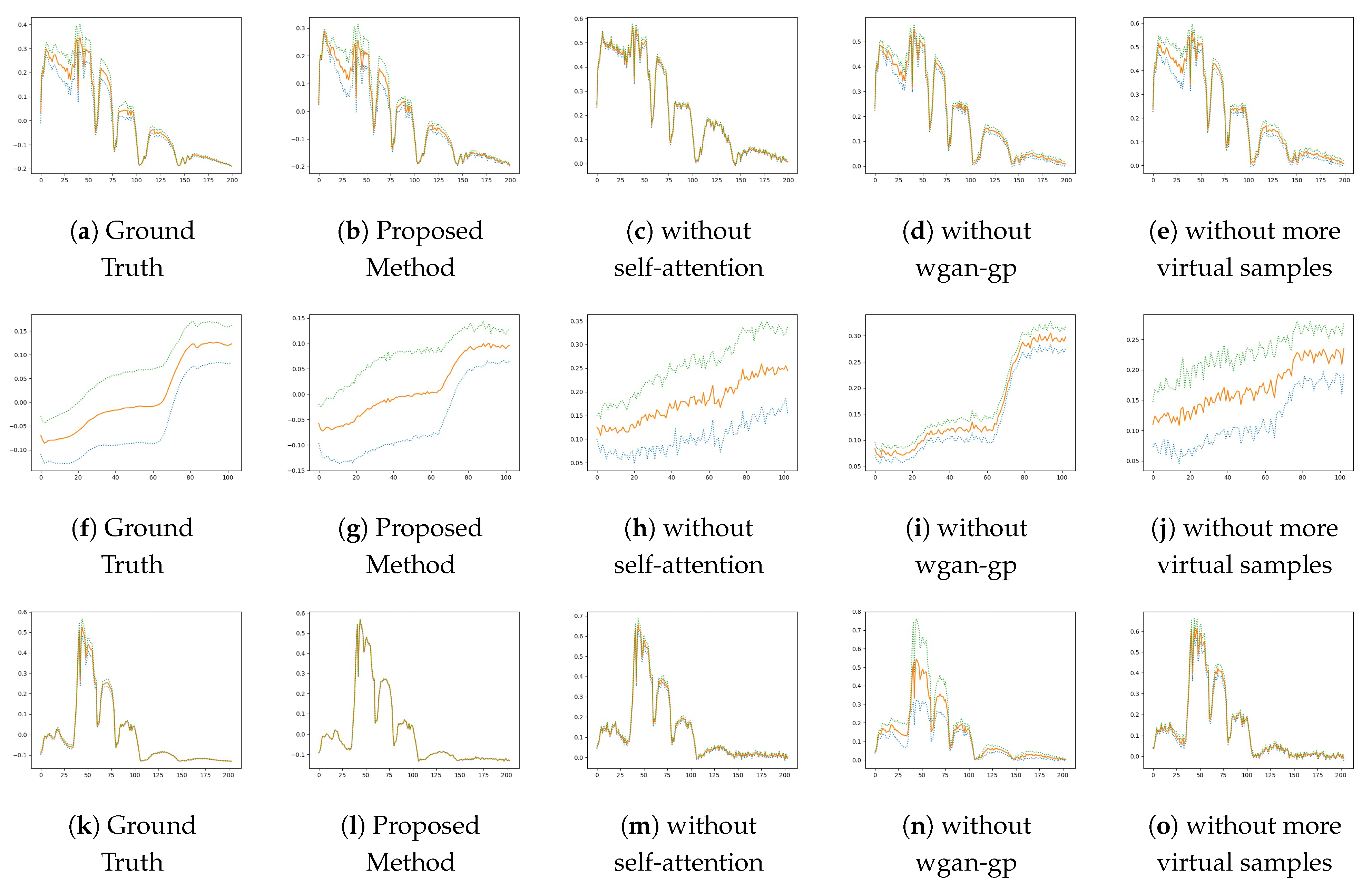
5.2. Spectral Feature Analysis
5.3. Overall Accuracy Analysis
6. Conclusions
Author Contributions
Funding
Conflicts of Interest
References
- Hong, D.; Yokoya, N.; Chanussot, J.; Zhu, X.X. An Augmented Linear Mixing Model to Address Spectral Variability for Hyperspectral Unmixing. IEEE Trans. Image Process. 2019, 28, 1923–1938. [Google Scholar] [CrossRef] [Green Version]
- Gevaert, C.M.; Suomalainen, J.; Tang, J.; Kooistra, L. Generation of Spectral–Temporal Response Surfaces by Combining Multispectral Satellite and Hyperspectral UAV Imagery for Precision Agriculture Applications. IEEE J. Sel. Top. Appl. Earth Obs. Remote Sens. 2015, 8, 3140–3146. [Google Scholar] [CrossRef]
- Hunt, E.R.; Daughtry, C.S.T.; Mirsky, S.B.; Hively, W.D. Remote Sensing With Simulated Unmanned Aircraft Imagery for Precision Agriculture Applications. IEEE J. Sel. Top. Appl. Earth Obs. Remote Sens. 2014, 7, 4566–4571. [Google Scholar] [CrossRef]
- Tao, C.; Wang, Y.J.; Zou, B.; Tu, Y.L.; Jiang, X.L. Assessment and Analysis of Migrations of Heavy Metal Lead and Zinc in Soil with Hyperspectral Inversion Model. Spectrosc. Spectr. Anal. 2018, 38, 1850. [Google Scholar]
- Wang, Q.; Yuan, Z.; Du, Q.; Li, X. GETNET: A General End-to-End 2-D CNN Framework for Hyperspectral Image Change Detection. IEEE Trans. Geosci. Remote Sens. 2019, 57, 3–13. [Google Scholar] [CrossRef] [Green Version]
- Salah Bourennane, C.F. Robust Denoising Method based on Tensor Models Decomposition for Hyperspectral Imagery. WSEAS Trans. Signal Process. 2019, 15, 92–98. [Google Scholar]
- Sawssen, B.; Okba, T.; Noureeddine, L. A Mammographic Images Classification Technique via the Gaussian Radial Basis Kernel ELM and KPCA. Int. J. Appl. Math. Comput. Sci. Syst. Eng. 2020, 2, 92–98. [Google Scholar]
- Vetova, S. A Comparative Study of Image Classification Models using NN and Similarity Distance. Int. J. Electr. Eng. Comput. Sci. (EEACS) 2021, 3, 109–113. [Google Scholar]
- Vetova, S. Covid Image Classification using Wavelet Feature Vectors and NN. Eng. World 2021, 3, 38–42. [Google Scholar]
- Luqman Hakim, M.I.Z. Implementation of Discrete Wavelet Transform on Movement Images and Recognition by Artificial Neural Network Algorithm. WSEAS Trans. Signal Process. 2019, 15, 149–154. [Google Scholar]
- Zhong, S.; Chang, C.I.; Zhang, Y. Iterative Support Vector Machine for Hyperspectral Image Classification. In Proceedings of the 2018 25th IEEE International Conference on Image Processing (ICIP), Athens, Greece, 7–10 October 2018; pp. 3309–3312. [Google Scholar]
- Sun, S.; Zhong, P.; Xiao, H.; Liu, F.; Wang, R. An active learning method based on SVM classifier for hyperspectral images classification. In Proceedings of the 2015 7th Workshop on Hyperspectral Image and Signal Processing: Evolution in Remote Sensing (WHISPERS), Tokyo, Japan, 2–5 June 2015; pp. 1–4. [Google Scholar]
- Melgani, F.; Bruzzone, L. Classification of hyperspectral remote sensing images with support vector machines. IEEE Trans. Geoence Remote Sens. 2004, 42, 1778–1790. [Google Scholar] [CrossRef] [Green Version]
- Song, W.; Li, S.; Kang, X.; Huang, K. Hyperspectral image classification based on KNN sparse representation. In Proceedings of the 2016 IEEE International Geoscience and Remote Sensing Symposium (IGARSS), Beijing, China, 10–15 July 2016; pp. 2411–2414. [Google Scholar]
- Guo, Y.; Cao, H.; Han, S.; Sun, Y.; Bai, Y. Spectral–Spatial HyperspectralImage Classification with K-Nearest Neighbor and Guided Filter. IEEE Access 2018, 6, 18582–18591. [Google Scholar] [CrossRef]
- Jia, X. Block-based maximum likelihood classification for hyperspectral remote sensing data. In Proceedings of the IGARSS’97. 1997 IEEE International Geoscience and Remote Sensing Symposium Proceedings: Remote Sensing—A Scientific Vision for Sustainable Development, Singapore, 3–8 August 1997; Volume 2, pp. 778–780. [Google Scholar]
- Ratle, F.; Camps-Valls, G.; Weston, J. Semisupervised Neural Networks for Efficient Hyperspectral Image Classification. IEEE Trans. Geosci. Remote Sens. 2010, 48, 2271–2282. [Google Scholar] [CrossRef]
- Li, J.; Bioucas-Dias, J.M.; Plaza, A. Semisupervised Hyperspectral Image Classification Using Soft Sparse Multinomial Logistic Regression. IEEE Geosci. Remote Sens. Lett. 2013, 10, 318–322. [Google Scholar]
- Khodadadzadeh, M.; Li, J.; Plaza, A.; Bioucas-Dias, J.M. A Subspace-Based Multinomial Logistic Regression for Hyperspectral Image Classification. IEEE Geosci. Remote Sens. Lett. 2014, 11, 2105–2109. [Google Scholar] [CrossRef]
- Hughes, G. On the mean accuracy of statistical pattern recognizers. IEEE Trans. Inf. Theory 1968, 14, 55–63. [Google Scholar] [CrossRef] [Green Version]
- Chen, Y.; Jiang, H.; Li, C.; Jia, X.; Ghamisi, P. Deep Feature Extraction and Classification of Hyperspectral Images Based on Convolutional Neural Networks. IEEE Trans. Geosci. Remote Sens. 2016, 54, 6232–6251. [Google Scholar] [CrossRef] [Green Version]
- Hamida, A.B.; Benoit, A.; Lambert, P.; Amar, C.B. 3-D Deep Learning Approach for Remote Sensing Image Classification. IEEE Trans. Geoence Remote Sens. 2018, 56, 4420–4434. [Google Scholar] [CrossRef] [Green Version]
- Chen, Y.; Wang, Y.; Gu, Y.; He, X.; Ghamisi, P.; Jia, X. Deep Learning Ensemble for Hyperspectral Image Classification. IEEE J. Sel. Top. Appl. Earth Obs. Remote Sens. 2019, 12, 1882–1897. [Google Scholar] [CrossRef]
- Chen, Y.; Lin, Z.; Zhao, X.; Wang, G.; Gu, Y. Deep Learning-Based Classification of Hyperspectral Data. IEEE J. Sel. Top. Appl. Earth Obs. Remote Sens. 2017, 7, 2094–2107. [Google Scholar] [CrossRef]
- Zhang, M.; Li, W.; Du, Q. Diverse Region-Based CNN for Hyperspectral Image Classification. IEEE Trans. Image Process. 2018, 27, 2623–2634. [Google Scholar] [CrossRef]
- Li, W.; Wu, G.; Zhang, F.; Du, Q. Hyperspectral Image Classification Using Deep Pixel-Pair Features. IEEE Trans. Geosci. Remote Sens. 2017, 55, 844–853. [Google Scholar] [CrossRef]
- Xu, X.; Li, W.; Ran, Q.; Du, Q.; Gao, L.; Zhang, B. Multisource Remote Sensing Data Classification Based on Convolutional Neural Network. IEEE Trans. Geosci. Remote Sens. 2018, 56, 937–949. [Google Scholar] [CrossRef]
- Xie, J.; He, N.; Fang, L.; Ghamisi, P. Multiscale Densely-Connected Fusion Networks for Hyperspectral Images Classification. IEEE Trans. Circuits Syst. Video Technol. 2021, 31, 246–259. [Google Scholar] [CrossRef]
- Ying, L.; Haokui, Z.; Qiang, S. Spectral-Spatial Classification of Hyperspectral Imagery with 3D Convolutional Neural Network. Remote Sens. 2017, 9, 67. [Google Scholar]
- Zhang, X.; Sun, Y.; Jiang, K.; Li, C.; Jiao, L.; Zhou, H. Spatial Sequential Recurrent Neural Network for Hyperspectral Image Classification. IEEE J. Sel. Top. Appl. Earth Obs. Remote Sens. 2018, 11, 4141–4155. [Google Scholar] [CrossRef] [Green Version]
- Yang, J.; Zhao, Y.; Chan, J.C.W.; Yi, C. Hyperspectral image classification using two-channel deep convolutional neural network. In Proceedings of the 2016 IEEE International Geoscience and Remote Sensing Symposium (IGARSS), Beijing, China, 10–15 July 2016; pp. 5079–5082. [Google Scholar]
- Goodfellow, I.; Pouget-Abadie, J.; Mirza, M.; Xu, B.; Warde-Farley, D.; Ozair, S.; Courville, A.; Bengio, Y. Generative Adversarial Networks. Commun. ACM 2020, 63, 139–144. [Google Scholar] [CrossRef]
- Wang, X.; Tan, K.; Du, Q.; Chen, Y.; Du, P. Caps-TripleGAN: GAN-Assisted CapsNet for Hyperspectral Image Classification. IEEE Trans. Geosci. Remote Sens. 2019, 57, 7232–7245. [Google Scholar] [CrossRef]
- Feng, J.; Yu, H.; Wang, L.; Cao, X.; Zhang, X.; Jiao, L. Classification of Hyperspectral Images Based on Multiclass Spatial–Spectral Generative Adversarial Networks. IEEE Trans. Geosci. Remote Sens. 2019, 57, 5329–5343. [Google Scholar] [CrossRef]
- Zhong, Z.; Li, J.; Clausi, D.A.; Wong, A. Generative Adversarial Networks and Conditional Random Fields for Hyperspectral Image Classification. IEEE Trans. Cybern. 2020, 50, 3318–3329. [Google Scholar]
- Zhu, L.; Chen, Y.; Ghamisi, P.; Benediktsson, J.A. Generative Adversarial Networks for Hyperspectral Image Classification. IEEE Trans. Geosci. Remote Sens. 2018, 56, 5046–5063. [Google Scholar] [CrossRef]
- Wang, H.; Tao, C.; Qi, J.; Li, H.; Tang, Y. Semi-Supervised Variational Generative Adversarial Networks for Hyperspectral Image Classification. In Proceedings of the IGARSS 2019—2019 IEEE International Geoscience and Remote Sensing Symposium, Yokohama, Japan, 28 July–2 August 2019; pp. 9792–9794. [Google Scholar]
- Zhang, F.; Bai, J.; Zhang, J.; Xiao, Z.; Pei, C. An Optimized Training Method for GAN-Based Hyperspectral Image Classification. IEEE Geosci. Remote Sens. Lett. 2020, 1–5. [Google Scholar] [CrossRef]
- Wang, W.Y.; Li, H.C.; Deng, Y.J.; Shao, L.Y.; Lu, X.Q.; Du, Q. Generative Adversarial Capsule Network With ConvLSTM for Hyperspectral Image Classification. IEEE Geosci. Remote Sens. Lett. 2021, 18, 523–527. [Google Scholar] [CrossRef]
- Yin, J.; Li, W.; Han, B. Hyperspectral Image Classification Based on Generative Adversarial Network with Dropblock. In Proceedings of the 2019 IEEE International Conference on Image Processing (ICIP), Taipei, Taiwan, 22–25 September 2019; pp. 405–409. [Google Scholar]
- Srivastava, N.; Hinton, G.; Krizhevsky, A.; Sutskever, I.; Salakhutdinov, R. Dropout: A Simple Way to Prevent Neural Networks from Overfitting. J. Mach. Learn. Res. 2014, 15, 1929–1958. [Google Scholar]
- Karras, T.; Aila, T.; Laine, S.; Lehtinen, J. Progressive growing of gans for improved quality, stability, and variation. arXiv 2017, arXiv:1710.10196. [Google Scholar]
- Gulrajani, I.; Ahmed, F.; Arjovsky, M.; Dumoulin, V.; Courville, C.A. Improved Training of Wasserstein GANs. In Proceedings of the Advances in Neural Information Processing Systems 30 (NIPS 2017), Long Beach, CA, USA, 4–9 December 2017; pp. 5767–5777. [Google Scholar]
- Sabour, S.; Frosst, N.; Hinton, G.E. Dynamic Routing Between Capsules. arXiv 2017, arXiv:1710.09829. [Google Scholar]
- Hochreiter, S.; Schmidhuber, J. Long short-term memory. Neural Comput. 1997, 9, 1735–1780. [Google Scholar] [CrossRef]
- Vaswani, A.; Shazeer, N.M.; Parmar, N.; Uszkoreit, J.; Jones, L.; Gomez, A.N.; Kaiser, L.; Polosukhin, I. Attention is All you Need. arXiv 2017, arXiv:1706.03762. [Google Scholar]
- Bao, J.; Chen, D.; Wen, F.; Li, H.; Hua, G. CVAE-GAN: Fine-Grained Image Generation through Asymmetric Training. In Proceedings of the IEEE International Conference on Computer Vision (ICCV), Venice, Italy, 22–29 October 2017; pp. 2764–2773. [Google Scholar]
- Zhang, H.; Goodfellow, I.; Metaxas, D.; Odena, A. Self-attention generative adversarial networks. In Proceedings of the International Conference on Machine Learning (PMLR 2019), Beach, CA, USA, 9–15 June 2019; pp. 7354–7363. [Google Scholar]
- Kingma, D.P.; Welling, M. Auto-Encoding Variational Bayes. arXiv 2014, arXiv:1312.6114. [Google Scholar]
- Mirza, M.; Osindero, S. Conditional Generative Adversarial Nets. arXiv 2014, arXiv:1411.1784. [Google Scholar]


| No. | Class | Training | Test |
|---|---|---|---|
| 1 | Alfalfa | 2 | 44 |
| 2 | Corn-notill | 71 | 1357 |
| 3 | Corn-mintill | 41 | 789 |
| 4 | Corn | 12 | 225 |
| 5 | Grass-pasture | 24 | 459 |
| 6 | Grass-trees | 37 | 693 |
| 7 | Grass-pasture-mowed | 1 | 27 |
| 8 | Hay-windrowed | 24 | 454 |
| 9 | Oats | 1 | 19 |
| 10 | Soybean-notill | 49 | 923 |
| 11 | Soybean-mintill | 123 | 2332 |
| 12 | Soybean-clean | 30 | 563 |
| 13 | Wheat | 10 | 195 |
| 14 | Woods | 63 | 1202 |
| 15 | Buildings-Grass-Trees-Drives | 19 | 367 |
| 16 | Stone-Steel-Towers | 5 | 88 |
| Total | 512 | 9737 |
| No. | Class | Training | Test |
|---|---|---|---|
| 1 | Asphalt | 132 | 6499 |
| 2 | Meadows | 373 | 18,276 |
| 3 | Gravel | 42 | 2057 |
| 4 | Trees | 61 | 3003 |
| 5 | Painted metal sheets | 27 | 1318 |
| 6 | Bare Soil | 100 | 4929 |
| 7 | Bitumen | 27 | 1303 |
| 8 | Self-Blocking Bricks | 74 | 3608 |
| 9 | Shadows | 19 | 928 |
| Total | 855 | 41,921 |
| No. | Class | Training | Test |
|---|---|---|---|
| 1 | Brocoli_green_weeds_1 | 20 | 1989 |
| 2 | Brocoli_green_weeds_2 | 37 | 3689 |
| 3 | Fallow | 20 | 1956 |
| 4 | Fallow_rough_plow | 14 | 1380 |
| 5 | Fallow_smooth | 27 | 2651 |
| 6 | Stubble | 39 | 3920 |
| 7 | Celery | 36 | 3543 |
| 8 | Grapes_untrained | 113 | 11,158 |
| 9 | Soil_vinyard_develop | 62 | 6141 |
| 10 | Corn_senesced_green_weeds | 33 | 3245 |
| 11 | Lettuce_romaine_4wk | 11 | 1057 |
| 12 | Lettuce_romaine_5wk | 19 | 1908 |
| 13 | Lettuce_romaine_6wk | 9 | 907 |
| 14 | Lettuce_romaine_7wk | 11 | 1059 |
| 15 | Vinyard_untrained | 72 | 7196 |
| 16 | Vinyard_vertical_trellis | 18 | 1789 |
| Total | 541 | 53,588 |
| Patch Size | Indian Pines | PaviaU | Salinas |
|---|---|---|---|
| 19 × 19 | 92.78 | 98.91 | 97.05 |
| 23 × 23 | 94.78 | 99.01 | 97.80 |
| 27 × 27 | 95.94 | 99.32 | 98.82 |
| 31 × 31 | 95.02 | 99.10 | 99.19 |
| Proposeed | Indian Pines | PaviaU | Salinas |
|---|---|---|---|
| None | 94.01 | 98.37 | 97.70 |
| Dropout | 95.26 | 98.26 | 98.00 |
| BN | 95.50 | 98.63 | 98.21 |
| Both | 95.94 | 99.32 | 98.82 |
| 0.5 | 0.6 | 0.7 | 0.8 | 0.9 | 1 | ||
|---|---|---|---|---|---|---|---|
| 0 | 94.50 | 94.82 | 95.23 | 95.73 | 95.67 | 95.39 | |
| 0.1 | 94.51 | 94.71 | 95.35 | 95.32 | 95.71 | 95.32 | |
| 0.2 | 93.56 | 94.75 | 95.46 | 95.94 | 95.76 | 95.44 | |
| 0.3 | 93.72 | 93.32 | 94.67 | 95.55 | 95.10 | 95.59 | |
| 0.4 | 93.85 | 94.10 | 94.43 | 94.57 | 94.66 | 94.91 | |
| 0.5 | 93.43 | 93.87 | 94.22 | 94.01 | 94.62 | 94.68 | |
| 0.5 | 0.6 | 0.7 | 0.8 | 0.9 | 1 | ||
|---|---|---|---|---|---|---|---|
| 0 | 98.99 | 99.01 | 99.05 | 99.24 | 99.10 | 98.82 | |
| 0.1 | 98.83 | 98.74 | 99.21 | 99.28 | 99.14 | 99.07 | |
| 0.2 | 98.91 | 99.12 | 99.27 | 99.32 | 99.29 | 99.19 | |
| 0.3 | 98.61 | 98.67 | 99.01 | 99.13 | 99.07 | 98.91 | |
| 0.4 | 98.69 | 98.43 | 98.87 | 98.57 | 98.76 | 98.59 | |
| 0.5 | 98.34 | 98.31 | 97.89 | 98.46 | 98.39 | 98.21 | |
| 0.5 | 0.6 | 0.7 | 0.8 | 0.9 | 1 | ||
|---|---|---|---|---|---|---|---|
| 0 | 98.47 | 98.51 | 98.57 | 98.65 | 98.41 | 98.61 | |
| 0.1 | 98.38 | 98.42 | 98.58 | 98.66 | 98.72 | 98.67 | |
| 0.2 | 98.46 | 98.32 | 98.78 | 98.82 | 98.81 | 98.79 | |
| 0.3 | 98.12 | 98.09 | 98.41 | 98.31 | 98.53 | 98.37 | |
| 0.4 | 97.75 | 98.18 | 98.43 | 98.29 | 98.05 | 98.17 | |
| 0.5 | 97.37 | 97.51 | 98.25 | 97.93 | 98.11 | 98.03 | |
| Class | SVM−RBF | Two−CNN | 3D−CNN | DCGAN | DBGAN | CVAEGAN | Proposed |
|---|---|---|---|---|---|---|---|
| 1 | 0 | 69.78 ± 1.98 | 17.70 ± 1.11 | 75.97 ± 0.04 | 37.83 ± 7.44 | 71.01 ± 2.37 | 66.67 ± 3.29 |
| 2 | 28.07 ± 2.63 | 84.78 ± 0.26 | 68.96 ± 0.84 | 85.60 ± 0.01 | 77.23 ± 1.38 | 90.13 ± 0.27 | 97.15 ± 0.38 |
| 3 | 0.33 ± 0.99 | 88.39 ± 0.59 | 68.11 ± 1.46 | 90.72 ± 0.01 | 81.16 ± 1.26 | 88.76 ± 0.91 | 91.04 ± 1.63 |
| 4 | 1.11 ± 2.90 | 94.68 ± 0.42 | 67.75 ± 3.67 | 95.36 ± 0.01 | 89.37 ± 3.95 | 90.44 ± 2.88 | 92.55 ± 1.80 |
| 5 | 2.11 ± 4.08 | 80.68 ± 0.75 | 87.52 ± 0.84 | 81.78 ± 0.02 | 24.43 ± 5.88 | 84.82 ± 2.06 | 91.58 ± 1.05 |
| 6 | 92.58 ± 2.35 | 95.04 ± 0.32 | 88.26 ± 0.65 | 95.62 ± 0.01 | 91.84 ± 0.97 | 99.45 ± 0.11 | 97.99 ± 0.31 |
| 7 | 0 | 90.00 ± 2.66 | 65.31 ± 6.28 | 81.07 ± 0.05 | 14.29 ± 9.16 | 79.76 ± 1.94 | 42.86 ± 2.92 |
| 8 | 99.21 ± 1.27 | 97.05 ± 0.22 | 99.16 ± 0.21 | 97.47 ± 0.00 | 98.42 ± 0.32 | 100 ± 0 | 98.60 ± 0.82 |
| 9 | 0 | 36.00 ± 0.63 | 60.00 ± 6.06 | 80.00 ± 0.04 | 29.50 ± 6.65 | 45.00 ± 4.08 | 38.33 ± 5.93 |
| 10 | 0.35 ± 1.04 | 84.44 ± 0.47 | 68.90 ± 0.77 | 87.14 ± 0.01 | 83.70 ± 0.69 | 89.27 ± 0.93 | 96.02 ± 1.3 |
| 11 | 94.99 ± 1.76 | 93.18 ± 0.27 | 80.14 ± 0.72 | 96.99 ± 0.00 | 94.12 ± 0.75 | 97.65 ± 0.64 | 98.56 ± 0.31 |
| 12 | 0.23 ± 0.54 | 82.48 ± 0.38 | 54.85 ± 2.36 | 83.98 ± 0.01 | 73.88 ± 2.44 | 85.83 ± 1.33 | 89.71 ± 0.68 |
| 13 | 0.29 ± 30.79 | 94.44 ± 0.46 | 98.47 ± 0.59 | 96.59 ± 0.01 | 95.41 ± 0.48 | 99.02 ± 0.61 | 99.84 ± 0.13 |
| 14 | 98.66 ± 0.38 | 96.17 ± 0.19 | 92.94 ± 0.36 | 98.18 ± 0.01 | 97.53 ± 0.40 | 99.31 ± 0.04 | 98.58 ± 0.78 |
| 15 | 2.70 ± 4.24 | 95.52 ± 0.62 | 69.73 ± 1.18 | 97.93 ± 0.02 | 87.42 ± 2.30 | 92.57 ± 2.20 | 95.51 ± 0.78 |
| 16 | 82.61 ± 4.37 | 84.95 ± 1.84 | 80.49 ± 2.10 | 88.17 ± 0.02 | 50.86 ± 8.51 | 78.49 ± 0.51 | 92.47 ± 2.63 |
| OA (%) | 51.69 ± 0.73 | 90.10 ± 0.21 | 77.80 ± 0.46 | 91.11 ± 0.45 | 84.42 ± 0.37 | 93.47 ± 0.11 | 95.94 ± 0.20 |
| AA (%) | 33.27 ± 1.75 | 85.41 ± 0.35 | 73.02 ± 0.73 | 87.53 ± 0.55 | 67.00 ± 0.29 | 86.97 ± 0.24 | 86.71 ± 0.69 |
| Kappa (%) | 41.46 ± 0.92 | 88.73 ± 0.24 | 74.68 ± 0.52 | 89.87 ± 0.51 | 82.14 ± 0.42 | 82.54 ± 0.13 | 95.36 ± 0.22 |
| Class | SVM−RBF | Two−CNN | 3D−CNN | DCGAN | DBGAN | CVAEGAN | Proposed |
|---|---|---|---|---|---|---|---|
| 1 | 91.49 ± 1.00 | 94.81 ± 0.16 | 96.91 ± 0.18 | 92.70 ± 0.35 | 96.03 ± 0.37 | 96.31 ± 0.53 | 99.60 ± 0.15 |
| 2 | 96.80 ± 2.76 | 99.51 ± 0.07 | 99.15 ± 0.08 | 99.40 ± 0.16 | 99.67 ± 0.09 | 99.98 ± 0.02 | 99.99 ± 0.01 |
| 3 | 1.89 ± 3.50 | 79.15 ± 0.28 | 85.88 ± 0.85 | 72.87 ± 3.10 | 80.98 ± 3.09 | 90.41 ± 0.68 | 97.09 ± 1.01 |
| 4 | 63.57 ± 12.59 | 94.14 ± 0.25 | 94.73 ± 0.45 | 91.33 ± 1.52 | 97.90 ± 0.33 | 95.96 ± 0.22 | 97.96 ± 0.44 |
| 5 | 98.87 ± 0.16 | 98.74 ± 0.34 | 99.72 ± 0.06 | 99.48 ± 0.16 | 98.23 ± 0.64 | 100 ± 0 | 100 ± 0 |
| 6 | 14.84 ± 1.79 | 96.88 ± 0.38 | 95.32 ± 0.49 | 96.34 ± 0.91 | 98.90 ± 0.31 | 99.25 ± 0.37 | 100 ± 0 |
| 7 | 0 | 84.09 ± 0.29 | 86.46 ± 0.99 | 85.41 ± 3.62 | 90.79 ± 1.29 | 94.29 ± 2.94 | 96.54 ± 1.95 |
| 8 | 91.90 ± 2.59 | 92.15 ± 0.24 | 94.41 ± 0.33 | 83.13 ± 0.20 | 93.83 ± 1.04 | 98.75 ± 0.26 | 98.23 ± 0.68 |
| 9 | 99.82 ± 0.08 | 92.73 ± 0.73 | 97.02 ± 0.54 | 86.91 ± 0.37 | 92.67 ± 1.79 | 90.11 ± 1.02 | 97.04 ± 0.85 |
| OA (%) | 76.00 ± 0.49 | 95.80 ± 0.09 | 96.55 ± 0.17 | 93.88 ± 0.39 | 96.99 ± 0.34 | 98.07 ± 0.04 | 99.32 ± 0.06 |
| AA (%) | 62.13 ± 1.16 | 92.47 ± 0.14 | 94.40 ± 0.33 | 89.19 ± 0.23 | 95.33 ± 0.21 | 96.12 ± 0.37 | 98.49 ± 0.14 |
| Kappa (%) | 66.28 ± 0.48 | 94.41 ± 0.12 | 95.42 ± 0.23 | 91.86 ± 0.51 | 96.00 ± 0.45 | 97.43 ± 0.05 | 99.10 ± 0.08 |
| Class | SVM−RBF | Two−CNN | 3D−CNN | DCGAN | DBGAN | CVAEGAN | Proposed |
|---|---|---|---|---|---|---|---|
| 1 | 94.92 ± 1.43 | 93.16 ± 0.61 | 97.58 ± 0.14 | 96.33 ± 1.10 | 23.48 ± 0.19 | 99.93 ± 0.05 | 99.30 ± 0.31 |
| 2 | 95.36 ± 1.43 | 98.79 ± 0.15 | 99.84 ± 0.04 | 92.39 ± 1.65 | 97.82 ± 1.49 | 100 ± 0 | 98.60 ± 0.57 |
| 3 | 60.68 ± 4.33 | 99.65 ± 0.16 | 98.46 ± 0.31 | 92.02 ± 1.36 | 98.50 ± 0.83 | 99.19 ± 0.45 | 99.85 ± 0.10 |
| 4 | 98.44 ± 0.36 | 96.90 ± 0.37 | 98.76 ± 0.24 | 97.20 ± 0.40 | 97.30 ± 0.58 | 97.87 ± 0.59 | 98.02 ± 0.77 |
| 5 | 96.83 ± 0.56 | 96.15 ± 0.20 | 87.56 ± 0.93 | 97.53 ± 0.50 | 96.03 ± 1.25 | 98.32 ± 0.33 | 99.22 ± 0.20 |
| 6 | 98.25 ± 0.79 | 98.65 ± 0.18 | 98.86 ± 0.24 | 91.02 ± 0.20 | 99.78 ± 0.11 | 99.99 ± 0.01 | 99.92 ± 0.03 |
| 7 | 99.05 ± 0.17 | 96.12 ± 0.32 | 98.10 ± 0.31 | 96.68 ± 0.58 | 98.70 ± 0.32 | 100 ± 0 | 99.95 ± 0.03 |
| 8 | 96.77 ± 2.87 | 94.22 ± 0.28 | 83.66 ± 0.69 | 81.53 ± 0.96 | 96.06 ± 0.58 | 97.23 ± 0.89 | 97.79 ± 0.36 |
| 9 | 98.65 ± 0.36 | 98.36 ± 0.13 | 97.29 ± 0.15 | 99.18 ± 0.33 | 98.82 ± 0.50 | 99.80 ± 0.17 | 99.44 ± 0.29 |
| 10 | 61.48 ± 11.90 | 99.78 ± 0.09 | 92.75 ± 0.53 | 97.87 ± 0.46 | 98.45 ± 0.36 | 99.30 ± 0.30 | 99.82 ± 0.13 |
| 11 | 0.11 ± 0.34 | 90.69 ± 0.24 | 89.96 ± 0.97 | 92.08 ± 1.63 | 63.55 ± 0.30 | 93.07 ± 0.54 | 96.47 ± 0.57 |
| 12 | 60.40 ± 7.68 | 91.99 ± 0.14 | 98.71 ± 0.26 | 91.26 ± 0.82 | 95.99 ± 0.80 | 97.61 ± 1.15 | 99.12 ± 0.47 |
| 13 | 38.82 ± 39.97 | 90.97 ± 0.54 | 98.76 ± 0.14 | 95.82 ± 0.92 | 94.07 ± 0.48 | 95.49 ± 1.28 | 96.98 ± 0.49 |
| 14 | 87.97 ± 1.71 | 93.90 ± 0.29 | 94.90 ± 0.35 | 96.50 ± 0.96 | 95.95 ± 0.78 | 97.69 ± 0.45 | 98.57 ± 0.45 |
| 15 | 2.91 ± 5.88 | 92.06 ± 0.19 | 75.98 ± 1.05 | 78.98 ± 1.68 | 97.93 ± 0.28 | 97.67 ± 0.30 | 98.81 ± 0.55 |
| 16 | 53.00 ± 3.16 | 99.23 ± 0.15 | 94.23 ± 1.14 | 81.08 ± 2.10 | 97.34 ± 0.80 | 98.73 ± 0.63 | 97.79 ± 0.47 |
| OA (%) | 75.25 ± 1.23 | 95.79 ± 0.07 | 91.05 ± 0.24 | 90.39 ± 0.35 | 94.13 ± 0.94 | 98.49 ± 0.01 | 98.82 ± 0.11 |
| AA (%) | 71.48 ± 3.01 | 95.66 ± 0.06 | 94.09 ± 0.19 | 92.80 ± 0.30 | 90.61 ± 2.34 | 98.24 ± 0.29 | 98.72 ± 0.08 |
| Kappa (%) | 71.92 ± 1.46 | 95.31 ± 0.07 | 90.04 ± 0.27 | 89.30 ± 0.39 | 93.46 ± 1.04 | 98.69 ± 0.12 | 98.80 ± 0.01 |
| Algorithms | Time | Indian Pines | PaviaU | Salinas |
|---|---|---|---|---|
| SVM−RBF | Train(s) | 0.0098 | 0.0080 | 0.0043 |
| Test(s) | 0.1366 | 0.4065 | 0.5430 | |
| Two−CNN | Train(s) | 2023.64 | 4306.78 | 10,957.61 |
| Test(s) | 22.47 | 48.75 | 140.63 | |
| 3D−CNN | Train(s) | 448.00 | 1565.82 | 2559.34 |
| Test(s) | 5.27 | 15.12 | 21.38 | |
| DCGAN | Train(s) | 7019.69 | 14,053.51 | 10,273.40 |
| Test(s) | 7.28 | 25.63 | 31.62 | |
| DBGAN | Train(s) | 3485.74 | 7922.47 | 6551.87 |
| Test(s) | 4.57 | 13.73 | 18.06 | |
| CVAEGAN | Train(s) | 4394.08 | 8514.97 | 6988.92 |
| Test(s) | 3.70 | 16.47 | 19.72 | |
| Proposed | Train(s) | 14,101.28 | 25,665.42 | 17,524.97 |
| Test(s) | 10.26 | 43.10 | 102.79 |
| Algorithms | Indian Pines | PaviaU | Salinas |
|---|---|---|---|
| SACVAEGAN without self-attention | 0.021 | 0.048 | 0.013 |
| SACVAEGAN without wgan-gp | 0.022 | 0.052 | 0.023 |
| SACVAEGAN without additional virtual samples | 0.020 | 0.046 | 0.021 |
| SACVAEGAN | 0.017 | 0.043 | 0.011 |
| Algorithms | Indian Pines | PaviaU | Salinas |
|---|---|---|---|
| SACVAEGAN without self-attention | 0.019 | 0.041 | 0.003 |
| SACVAEGAN without wgan-gp | 0.012 | 0.021 | 0.028 |
| SACVAEGAN without additional virtual samples | 0.011 | 0.035 | 0.011 |
| SACVAEGAN | 0.011 | 0.014 | 0.002 |
| Algorithms | Indian Pines | PaviaU | Salinas |
|---|---|---|---|
| SACVAEGAN without self-attention | 95.37 | 98.52 | 98.38 |
| SACVAEGAN without wgan-gp | 95.61 | 99.01 | 98.67 |
| SACVAEGAN without additional virtual samples | 95.43 | 98.99 | 98.64 |
| SACVAEGAN | 95.94 | 99.32 | 98.82 |
| Algorithms | Indian Pines | PaviaU | Salinas |
|---|---|---|---|
| SACVAEGAN | 10.21 | 1.78 | 2.37 |
| SACVAEGAN without wgan-gp | 12.35 | 12.62 | 11.83 |
Publisher’s Note: MDPI stays neutral with regard to jurisdictional claims in published maps and institutional affiliations. |
© 2021 by the authors. Licensee MDPI, Basel, Switzerland. This article is an open access article distributed under the terms and conditions of the Creative Commons Attribution (CC BY) license (https://creativecommons.org/licenses/by/4.0/).
Share and Cite
Chen, Z.; Tong, L.; Qian, B.; Yu, J.; Xiao, C. Self-Attention-Based Conditional Variational Auto-Encoder Generative Adversarial Networks for Hyperspectral Classification. Remote Sens. 2021, 13, 3316. https://0-doi-org.brum.beds.ac.uk/10.3390/rs13163316
Chen Z, Tong L, Qian B, Yu J, Xiao C. Self-Attention-Based Conditional Variational Auto-Encoder Generative Adversarial Networks for Hyperspectral Classification. Remote Sensing. 2021; 13(16):3316. https://0-doi-org.brum.beds.ac.uk/10.3390/rs13163316
Chicago/Turabian StyleChen, Zhitao, Lei Tong, Bin Qian, Jing Yu, and Chuangbai Xiao. 2021. "Self-Attention-Based Conditional Variational Auto-Encoder Generative Adversarial Networks for Hyperspectral Classification" Remote Sensing 13, no. 16: 3316. https://0-doi-org.brum.beds.ac.uk/10.3390/rs13163316