
Rupture Kinematics and Coseismic Slip Model of the 2021 Mw 7.3 Maduo (China) Earthquake: Implications for the Seismic Hazard of the Kunlun Fault


Abstract
:
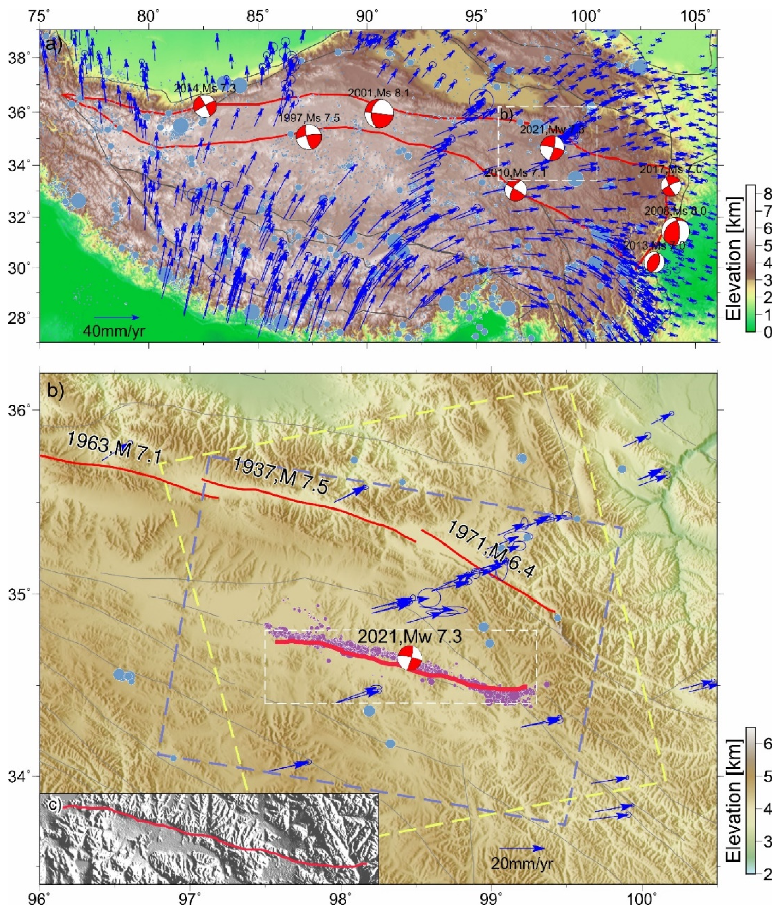
1. Introduction
2. Data and Methods
2.1. InSAR Data and Processing
2.2. Three-Dimensional Displacement Field Decomposing
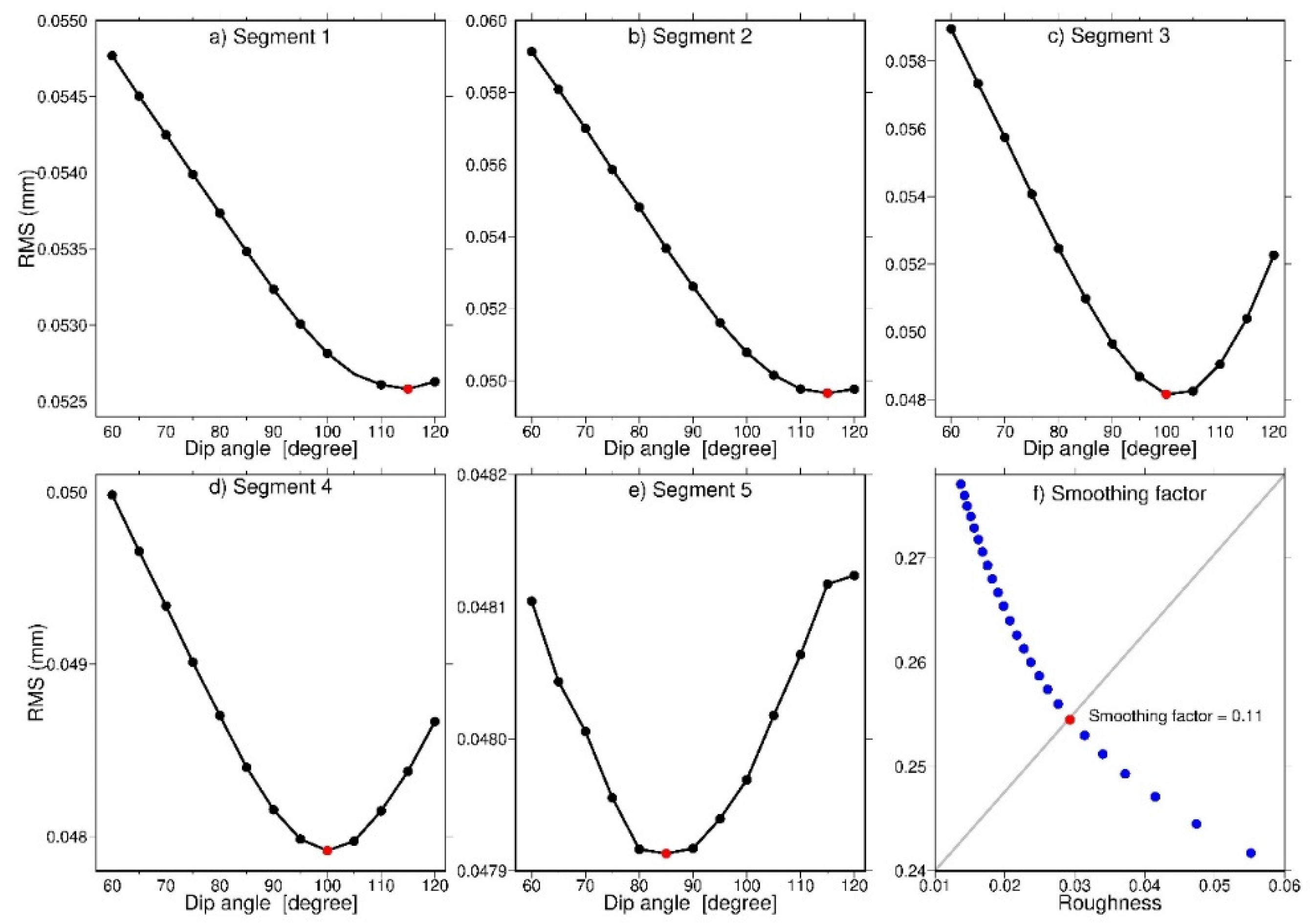
2.3. Slip Distribution Inversion Method
3. Results
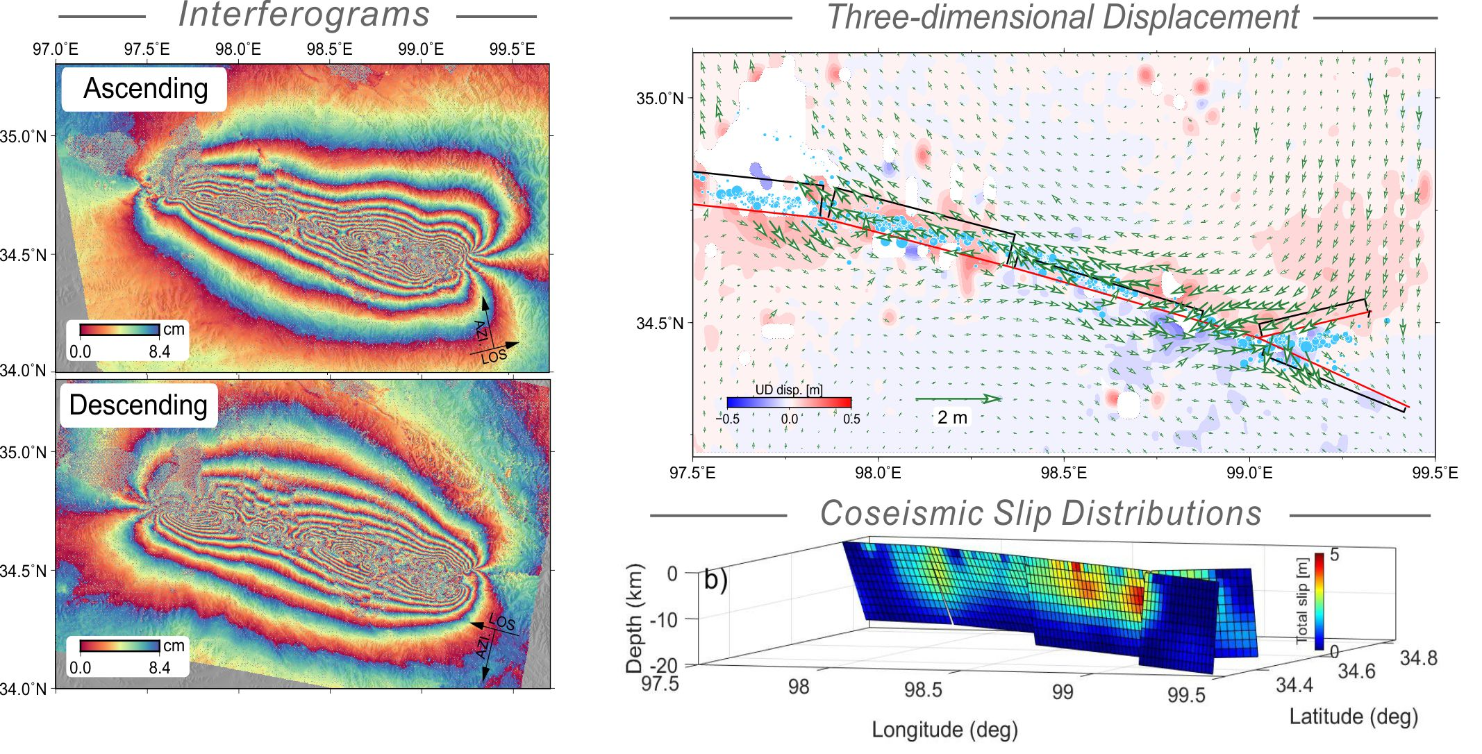
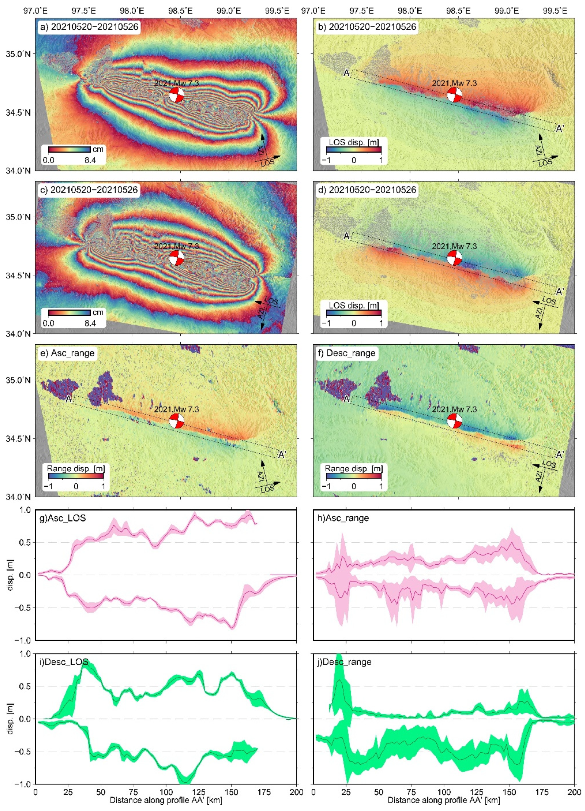
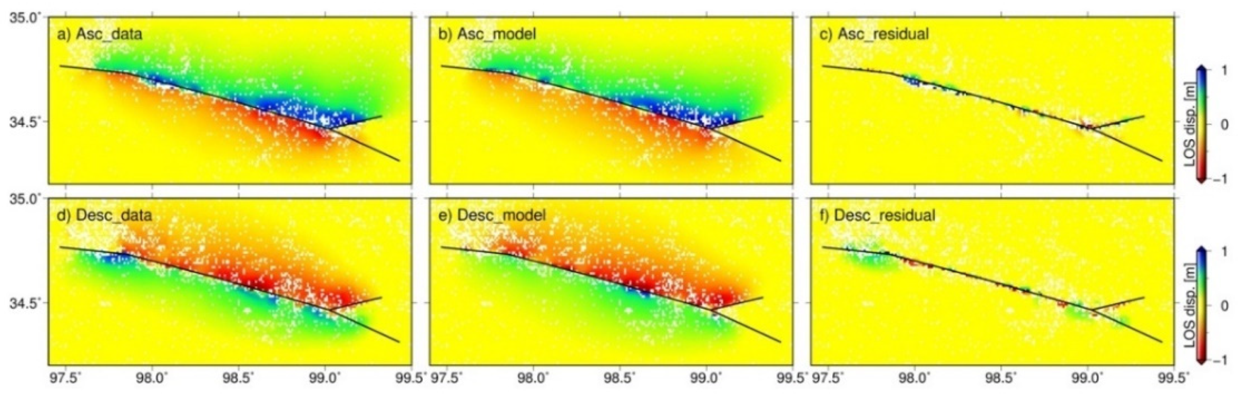
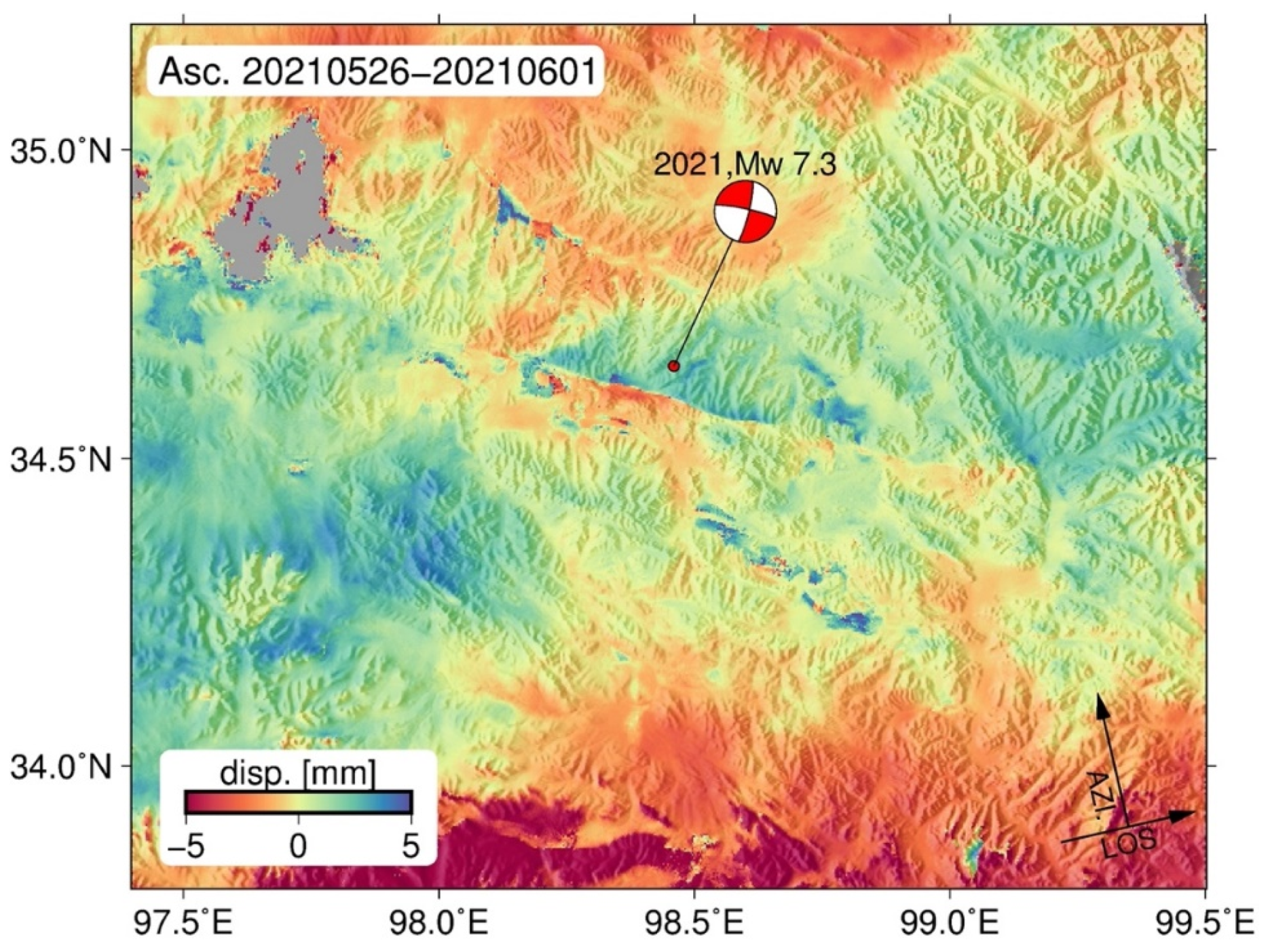
3.1. Coseismic Deformation Fields
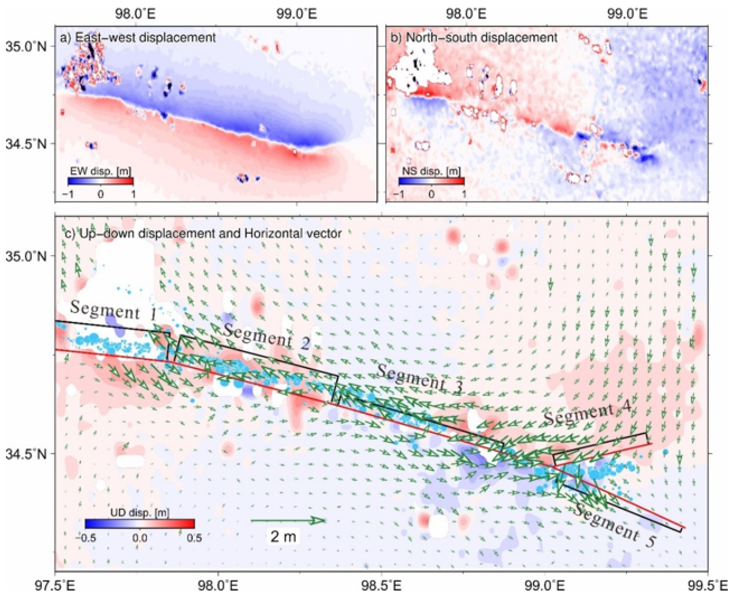
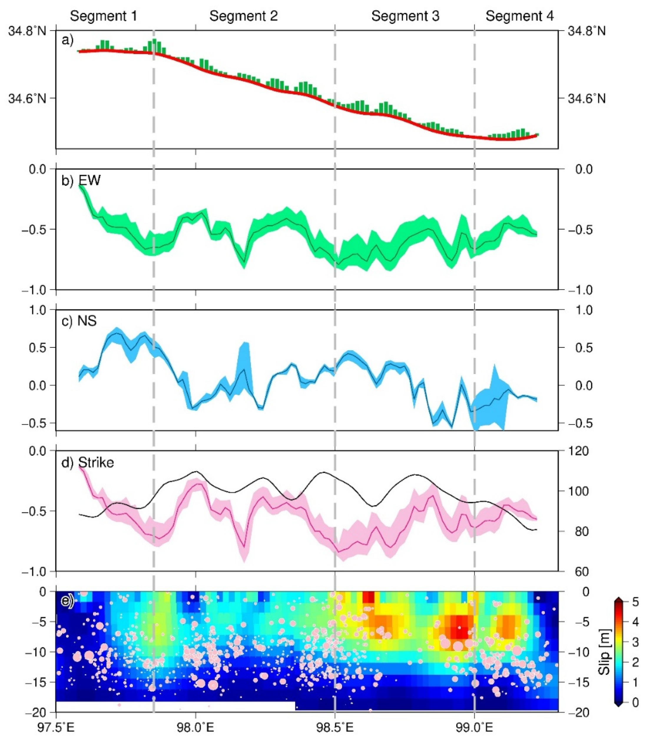
3.2. Complete Three Dimensional Displacement Fields
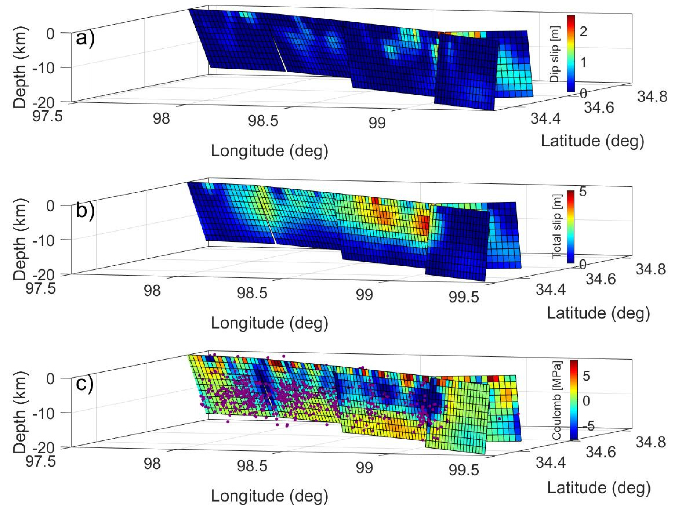
3.3. Fault Geometry and Coseismic Slip Distributions
4. Discussion
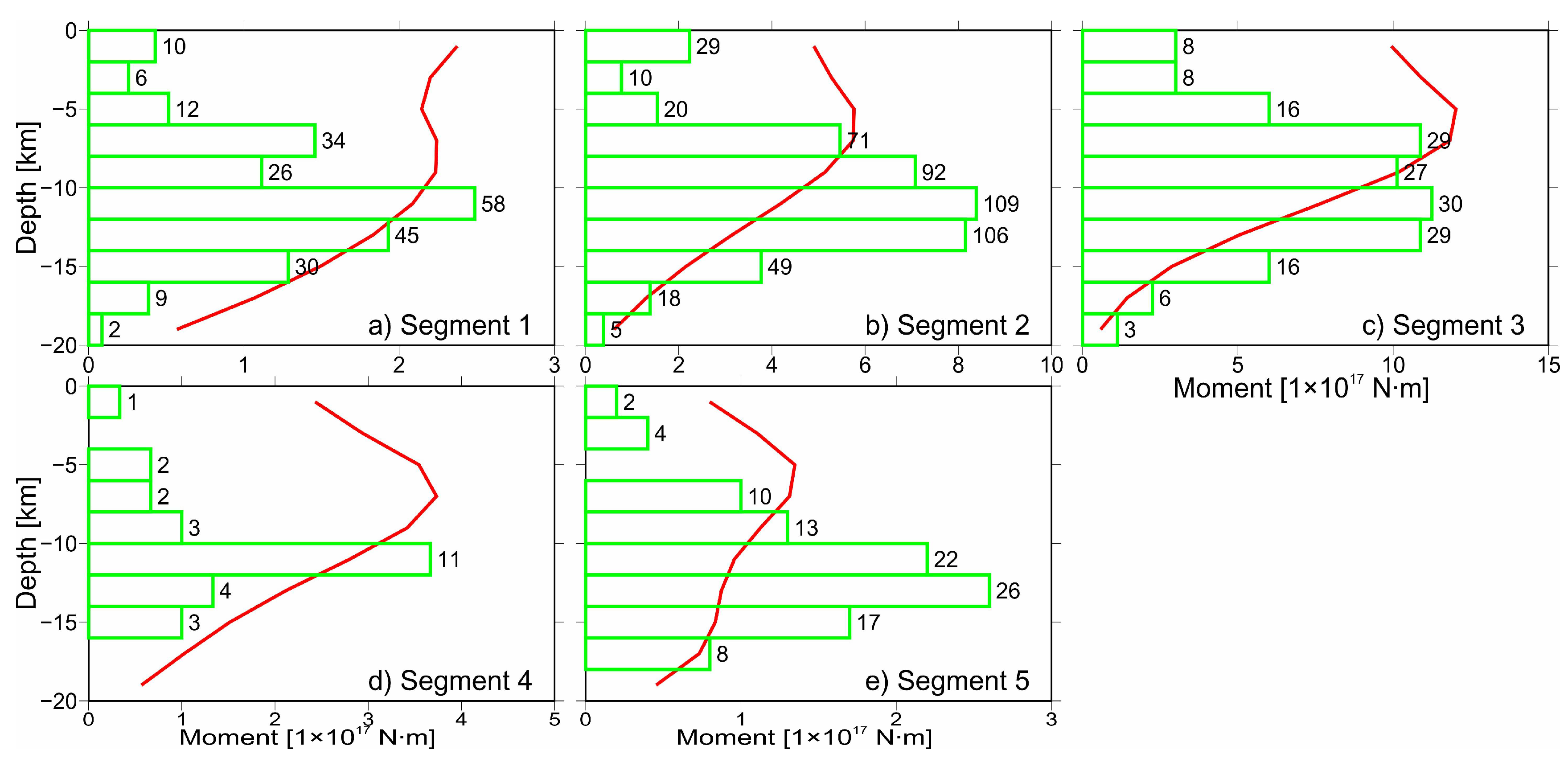
4.1. Depth Distribution of Coseismic Slip and Aftershocks
4.2. Implications on Seismic Hazard Estimate for the Kunlun Fault
5. Conclusions
Author Contributions
Funding
Institutional Review Board Statement
Informed Consent Statement
Data Availability Statement
Acknowledgments
Conflicts of Interest
References
- Xiong, X.; Shan, B.; Zheng, Y.; Wang, R. Stress transfer and its implication for earthquake hazard on the Kunlun Fault, Tibet. Tectonophysics 2010, 482, 216–225. [Google Scholar] [CrossRef] [Green Version]
- Junlong, Z. On fault evidence for a large earthquake in the late fifteenth century, Eastern Kunlun fault, China. J. Seismol. 2017, 21, 1397–1405. [Google Scholar] [CrossRef]
- Zhu, L.; Ji, L.; Jiang, F. Variations in Locking Along the East Kunlun Fault, Tibetan Plateau, China, Using GPS and Leveling Data. Pure Appl. Geophys. 2019, 177, 215–231. [Google Scholar] [CrossRef]
- Zhan, Y.; Liang, M.; Sun, X.; Huang, F.; Zhao, L.; Gong, Y.; Han, J.; Li, C.; Zhang, P.; Zhang, H. Deep structure and seismogenic pattern of the 2021.5.22 Madoi (Qinghai) MS7.4 earthquake. Chin. J. Geophys. 2021, 64, 2232–2252. (In Chinese) [Google Scholar] [CrossRef]
- Qu, W.; Lu, Z.; Zhang, Q.; Hao, M.; Wang, Q.; Qu, F.; Zhu, W. Present-day crustal deformation characteristics of the southeastern Tibetan Plateau and surrounding areas by using GPS analysis. J. Asian Earth Sci. 2018, 163, 22–31. [Google Scholar] [CrossRef]
- Ji, L.; Zhang, W.; Liu, C.; Zhu, L.; Xu, J.; Xu, X. Characterizing interseismic deformation of the Xianshuihe fault, eastern Tibetan Plateau, using Sentinel-1 SAR images. Adv. Space Res. 2020, 66, 378–394. [Google Scholar] [CrossRef]
- Li, H.; Van der Woerd, J.; Tapponnier, P.; Klinger, Y.; Qi, X.; Yang, J.; Zhu, Y. Slip rate on the Kunlun fault at Hongshui Gou, and recurrence time of great events comparable to the 14/11/2001, Mw∼7.9 Kokoxili earthquake. Earth Planet. Sci. Lett. 2005, 237, 285–299. [Google Scholar] [CrossRef]
- Yan, B.; Lin, A. Systematic deflection and offset of the Yangtze River drainage system along the strike-slip Ganzi-Yushu-Xianshuihe Fault Zone, Tibetan Plateau. J. Geodyn. 2015, 87, 13–25. [Google Scholar] [CrossRef]
- Van der Woerd, J.; Ryerson, F.J.; Tapponnier, P.; Gaudemer, Y.; Finkel, R.; Meriaux, A.S.; Caffee, M.; Guoguang, Z.; Qunlu, H. Holocene left-slip rate determined by cosmogenic surface dating on the Xidatan segment of the Kunlun fault (Qinghai, China). Geology 1998, 26, 695–698. [Google Scholar] [CrossRef] [Green Version]
- Van der Woerd, J.; Ryerson, F.J.; Tapponnier, P.; Meriaux, A.S.; Gaudemer, Y.; Meyer, B.; Finkel, R.C.; Caffee, M.W.; Guoguang, Z.; Zhiqin, X. Uniform slip-rate along the Kunlun Fault: Implications for seismic behaviour and large-scale tectonics. Geophys. Res. Lett. 2000, 27, 2353–2356. [Google Scholar] [CrossRef] [Green Version]
- Der Woerd, J.V.; Tapponnier, P.; Ryerson, F.J.; Meriaux, A.-S.; Meyer, B.; Gaudemer, Y.; Finkel, R.C.; Caffee, M.W.; Guoguan, Z.; Zhiqin, X. Uniform postglacial slip-rate along the central 600 km of the Kunlun Fault (Tibet), from 26Al, 10Be, and 14C dating of riser offsets, and climatic origin of the regional morphology. Geophys. J. Int. 2002, 148, 356–388. [Google Scholar] [CrossRef]
- Wang, H.; Wright, T.J.; Biggs, J. Interseismic slip rate of the northwestern Xianshuihe fault from InSAR data. Geophys. Res. Lett. 2009, 36. [Google Scholar] [CrossRef]
- Chevalier, M.-L.; Leloup, P.H.; Replumaz, A.; Pan, J.; Métois, M.; Li, H. Temporally constant slip rate along the Ganzi fault, NW Xianshuihe fault system, eastern Tibet. GSA Bull. 2017, 130, 396–410. [Google Scholar] [CrossRef]
- Zhu, L.; Ji, L.; Liu, C. Interseismic slip rate and locking along the Maqin–Maqu Segment of the East Kunlun Fault, Northern Tibetan Plateau, based on Sentinel-1 images. J. Asian Earth Sci. 2021, 211, 104703. [Google Scholar] [CrossRef]
- Parsons, T.; Toda, S.; Stein, R.S.; Barka, A.; Dieterich, J.H. Heightened odds of large earthquakes near Istanbul: An interaction-based probability calculation. Science 2000, 288, 661–665. [Google Scholar] [CrossRef] [Green Version]
- Zhao, L.; Qu, C.; Shan, X.; Zhao, D.; Gong, W.; Li, Y. Coseismic deformation and multi-fault slip model of the 2019 Mindanao earthquake sequence derived from Sentinel-1 and ALOS-2 data. Tectonophysics 2021, 799, 228707. [Google Scholar] [CrossRef]
- Li, Z.; Li, W.; Li, T.; Xu, Y.; Su, P.; Guo, P.; Sun, Y.; Ha, G.; Chen, G.; Yao, Z.; et al. Seismogenic fault and coseismic surface deformation of the Maduo Ms7.4 earthquake in Qinghai, China: A quick report. Seismol. Geol. 2021, 43, 722–737. (In Chinese) [Google Scholar] [CrossRef]
- Wang, M.; Shen, Z.K. Present-Day Crustal Deformation of Continental China Derived from GPS and Its Tectonic Implications. J. Geophys. Res. Solid Earth 2020, 125, e2019JB018774. [Google Scholar] [CrossRef] [Green Version]
- Diao, F.; Xiong, X.; Wang, R.; Walter, T.R.; Wang, Y.; Wang, K. Slip Rate Variation Along the Kunlun Fault (Tibet): Results from New GPS Observations and a Viscoelastic Earthquake-Cycle Deformation Model. Geophys. Res. Lett. 2019, 46, 2524–2533. [Google Scholar] [CrossRef]
- Wang, W.; Fang, L.; Wu, J.; Tu, H.; Zhang, L. Aftershock sequence relocation of the 2021 Ms7.4 Maduo Earthquake, Qinghai, China. Sci. China Earth Sci. 2021, 64, 1371–1380. [Google Scholar] [CrossRef]
- Werner, C.; Wegmüller, U.; Strozzi, T.; Wiesmann, A. Gamma SAR and interferometric processing software. Proc. Ers-Envisat Symp. Gothenbg. Swed. 2000, 1620, 1620. [Google Scholar]
- Prats-Iraola, P.; Scheiber, R.; Marotti, L.; Wollstadt, S.; Reigber, A. TOPS Interferometry With TerraSAR-X. IEEE Trans. Geosci. Remote Sens. 2012, 50, 3179–3188. [Google Scholar] [CrossRef] [Green Version]
- Goldstein, R.M.; Werner, C.L. Radar interferogram filtering for geophysical applications. Geophys. Res. Lett. 1998, 25, 4035–4038. [Google Scholar] [CrossRef] [Green Version]
- Hu, J.; Li, Z.W.; Ding, X.L.; Zhu, J.J.; Zhang, L.; Sun, Q. Resolving three-dimensional surface displacements from InSAR measurements: A review. Earth-Sci. Rev. 2014, 133, 1–17. [Google Scholar] [CrossRef]
- Liu, J.-H.; Hu, J.; Li, Z.-W.; Zhu, J.-J.; Sun, Q.; Gan, J. A Method for Measuring 3-D Surface Deformations With InSAR Based on Strain Model and Variance Component Estimation. IEEE Trans. Geosci. Remote Sens. 2018, 56, 239–250. [Google Scholar] [CrossRef]
- Wang, R.; Parolai, S.; Ge, M.; Jin, M.; Walter, T.R.; Zschau, J. The 2011 Mw 9.0 Tohoku Earthquake: Comparison of GPS and Strong-Motion Data. Bull. Seismol. Soc. Am. 2013, 103, 1336–1347. [Google Scholar] [CrossRef]
- Feng, W.; Li, Z.; Elliott, J.R.; Fukushima, Y.; Hoey, T.; Singleton, A.; Cook, R.; Xu, Z. The 2011 MW 6.8 Burma earthquake: Fault constraints provided by multiple SAR techniques. Geophys. J. Int. 2013, 195, 650–660. [Google Scholar] [CrossRef] [Green Version]
- Milliner, C.; Donnellan, A.; Aati, S.; Avouac, J.-P.; Zinke, R.; Dolan, J.F.; Wang, K.; Bürgmann, R. Bookshelf Kinematics and the Effect of Dilatation on Fault Zone Inelastic Deformation: Examples From Optical Image Correlation Measurements of the 2019 Ridgecrest Earthquake Sequence. J. Geophys. Res. Solid Earth 2021, 126, e2020JB020551. [Google Scholar] [CrossRef]
- Rice, J.R.; Tse, S.T. Dynamic motion of a single degree of freedom system following a rate and state dependent friction law. J. Geophys. Res. Solid Earth 1986, 91, 521–530. [Google Scholar] [CrossRef]
- Rice, J.R. Spatio-temporal complexity of slip on a fault. J. Geophys. Res. Solid Earth 1993, 98, 9885–9907. [Google Scholar] [CrossRef] [Green Version]
- Kaneko, Y.; Fialko, Y. Shallow slip deficit due to large strike-slip earthquakes in dynamic rupture simulations with elasto-plastic off-fault response. Geophys. J. Int. 2011, 186, 1389–1403. [Google Scholar] [CrossRef] [Green Version]
- Fialko, Y.; Sandwell, D.; Simons, M.; Rosen, P. Three-dimensional deformation caused by the Bam, Iran, earthquake and the origin of shallow slip deficit. Nature 2005, 435, 295–299. [Google Scholar] [CrossRef] [PubMed]
- Fielding, E.J.; Lundgren, P.R.; Burgmann, R.; Funning, G.J. Shallow fault-zone dilatancy recovery after the 2003 Bam earthquake in Iran. Nature 2009, 458, 64–68. [Google Scholar] [CrossRef]
- Marone, C.J.; Scholtz, C.H.; Bilham, R. On the mechanics of earthquake afterslip. J. Geophys. Res. 1991, 96, 8441–8452. [Google Scholar] [CrossRef]
- McCloskey, J.; Nalbant, S.S.; Steacy, S. Earthquake risk from co-seismic stress. Nature 2005, 434, 291. [Google Scholar] [CrossRef]
- Perfettini, H.; Avouac, J.P. Modeling afterslip and aftershocks following the 1992 Landers earthquake. J. Geophys. Res. 2007, 112. [Google Scholar] [CrossRef]
- Wessel, P.; Smith, W.H.F.; Scharroo, R.; Luis, J.; Wobbe, F. Generic Mapping Tools: Improved Version Released. Eos Trans. Am. Geophys. Union 2013, 94, 409–410. [Google Scholar] [CrossRef] [Green Version]


| Orbit | Track | Acquisition Date | Perpendicular Baseline (m) | Incidence Angle (°) | Heading (°) | |
|---|---|---|---|---|---|---|
| Reference Image | Secondary Image | |||||
| Ascending | 106 | 20 May 2021 | 26 May 2021 | −0.36 | 33~43 | −13 |
| Descending | 99 | 20 May 2021 | 26 May 2021 | 3.22 | 33~43 | −144 |
| Source | Mw | Focal Depth (km) | Longitude (°) | Latitude (°) | Strike (°) | Dip (°) | Rake (°) |
|---|---|---|---|---|---|---|---|
| GCMT | 7.4 | 12 | 98.46 | 34.65 | 282 | 83 | −9 |
| USGS | 7.3 | 10 | 98.2458 | 34.6125 | 92 | 67 | −40 |
Publisher’s Note: MDPI stays neutral with regard to jurisdictional claims in published maps and institutional affiliations. |
© 2021 by the authors. Licensee MDPI, Basel, Switzerland. This article is an open access article distributed under the terms and conditions of the Creative Commons Attribution (CC BY) license (https://creativecommons.org/licenses/by/4.0/).
Share and Cite
Chen, H.; Qu, C.; Zhao, D.; Ma, C.; Shan, X. Rupture Kinematics and Coseismic Slip Model of the 2021 Mw 7.3 Maduo (China) Earthquake: Implications for the Seismic Hazard of the Kunlun Fault. Remote Sens. 2021, 13, 3327. https://0-doi-org.brum.beds.ac.uk/10.3390/rs13163327
Chen H, Qu C, Zhao D, Ma C, Shan X. Rupture Kinematics and Coseismic Slip Model of the 2021 Mw 7.3 Maduo (China) Earthquake: Implications for the Seismic Hazard of the Kunlun Fault. Remote Sensing. 2021; 13(16):3327. https://0-doi-org.brum.beds.ac.uk/10.3390/rs13163327
Chicago/Turabian StyleChen, Han, Chunyan Qu, Dezheng Zhao, Chao Ma, and Xinjian Shan. 2021. "Rupture Kinematics and Coseismic Slip Model of the 2021 Mw 7.3 Maduo (China) Earthquake: Implications for the Seismic Hazard of the Kunlun Fault" Remote Sensing 13, no. 16: 3327. https://0-doi-org.brum.beds.ac.uk/10.3390/rs13163327