
Understanding Spatio-Temporal Patterns of Land Use/Land Cover Change under Urbanization in Wuhan, China, 2000–2019


Abstract
:1. Introduction
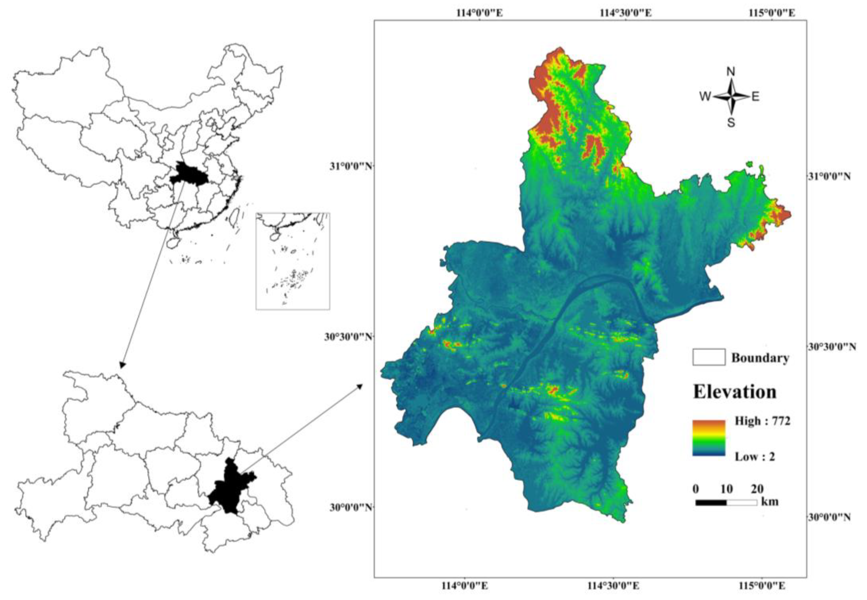
2. Study Area and Data Resources
2.1. Study Area
2.2. Data Resources
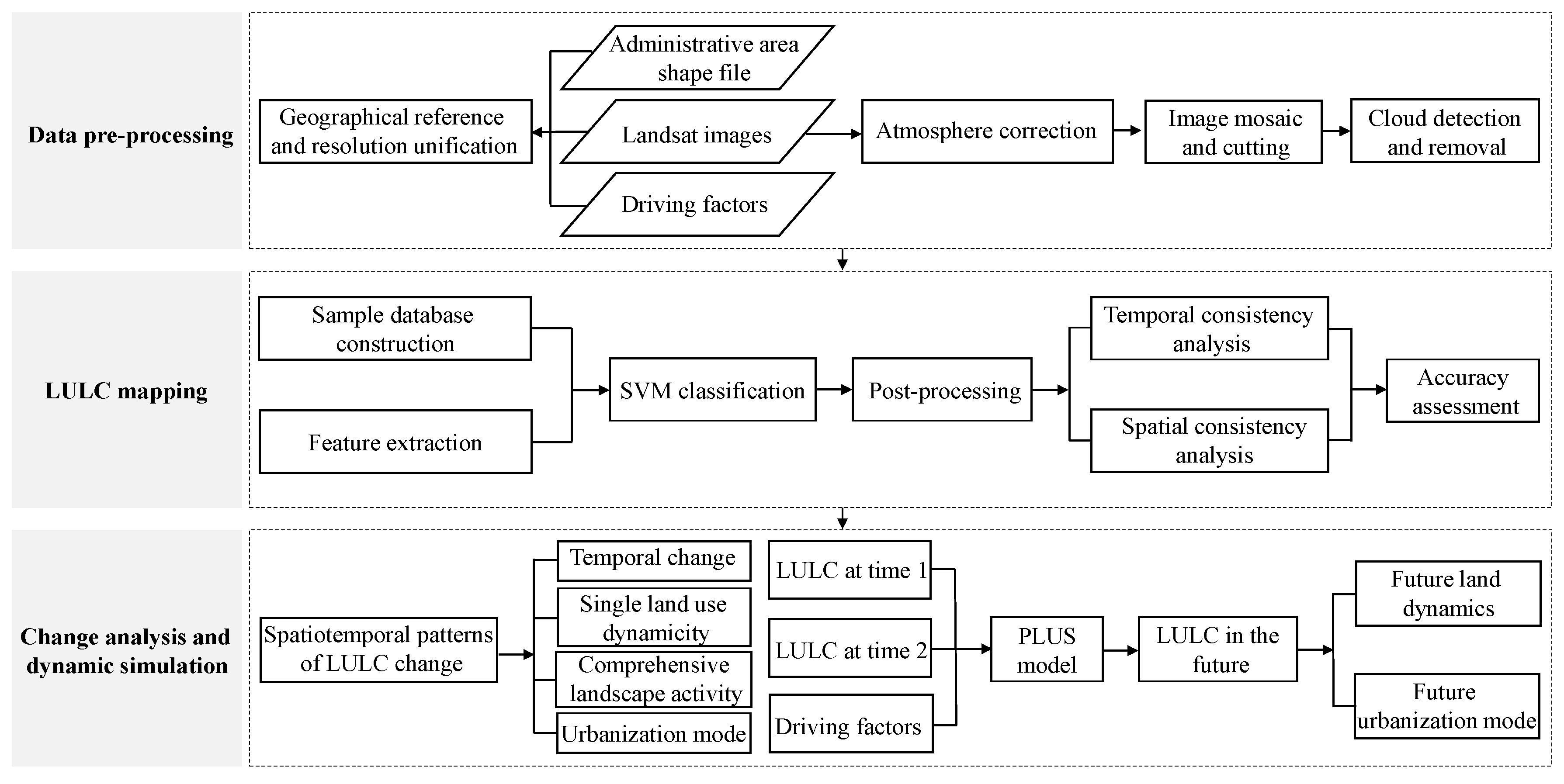
3. Method
3.1. Data Pre-Processing
3.2. LULC Mapping
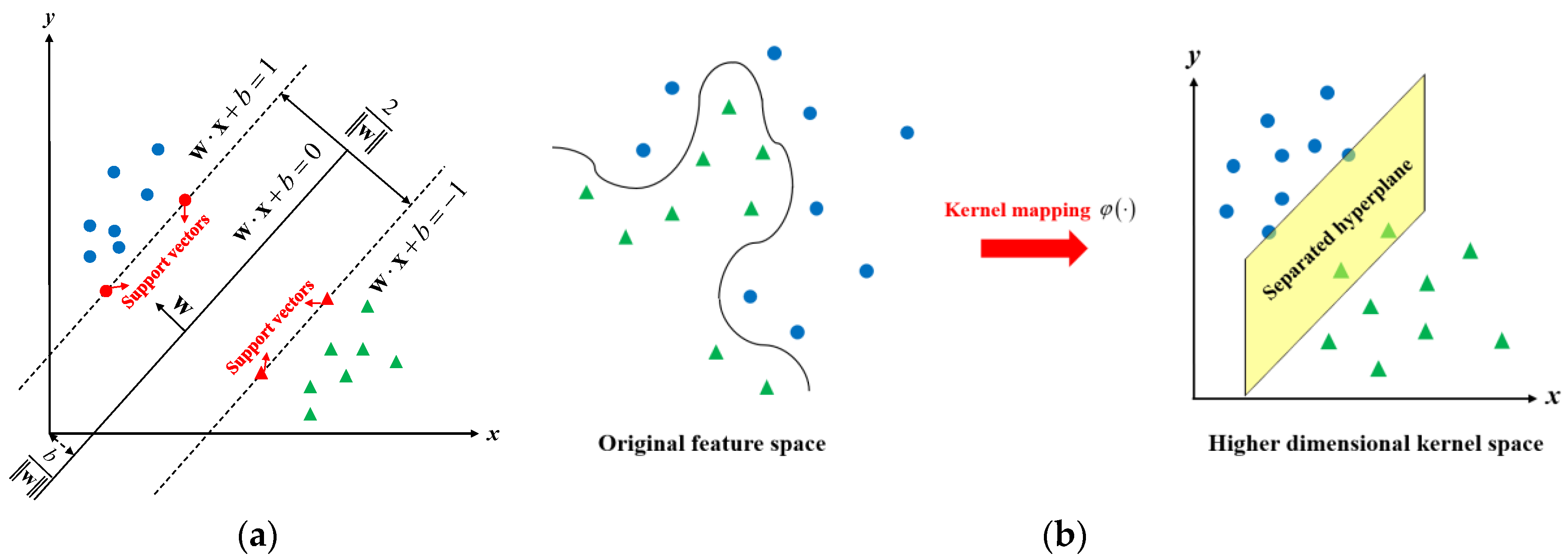
3.2.1. Feature Extraction and Classification
3.2.2. Post-Processing
3.3. LULC Change Analysis and Modeling
3.4. LULC Dynamic Simulation
4. Results
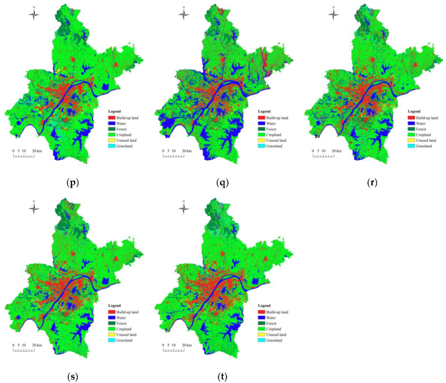
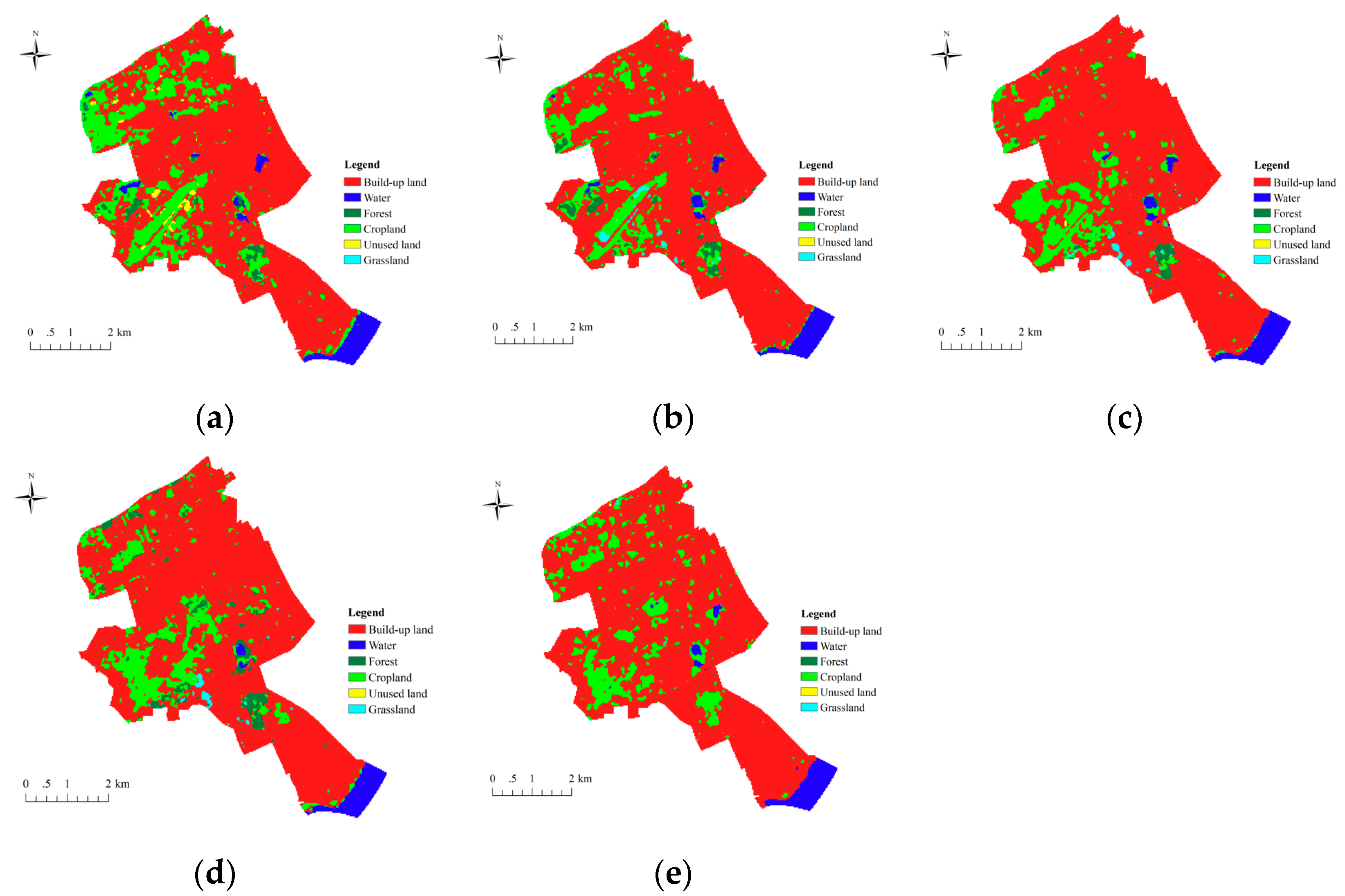
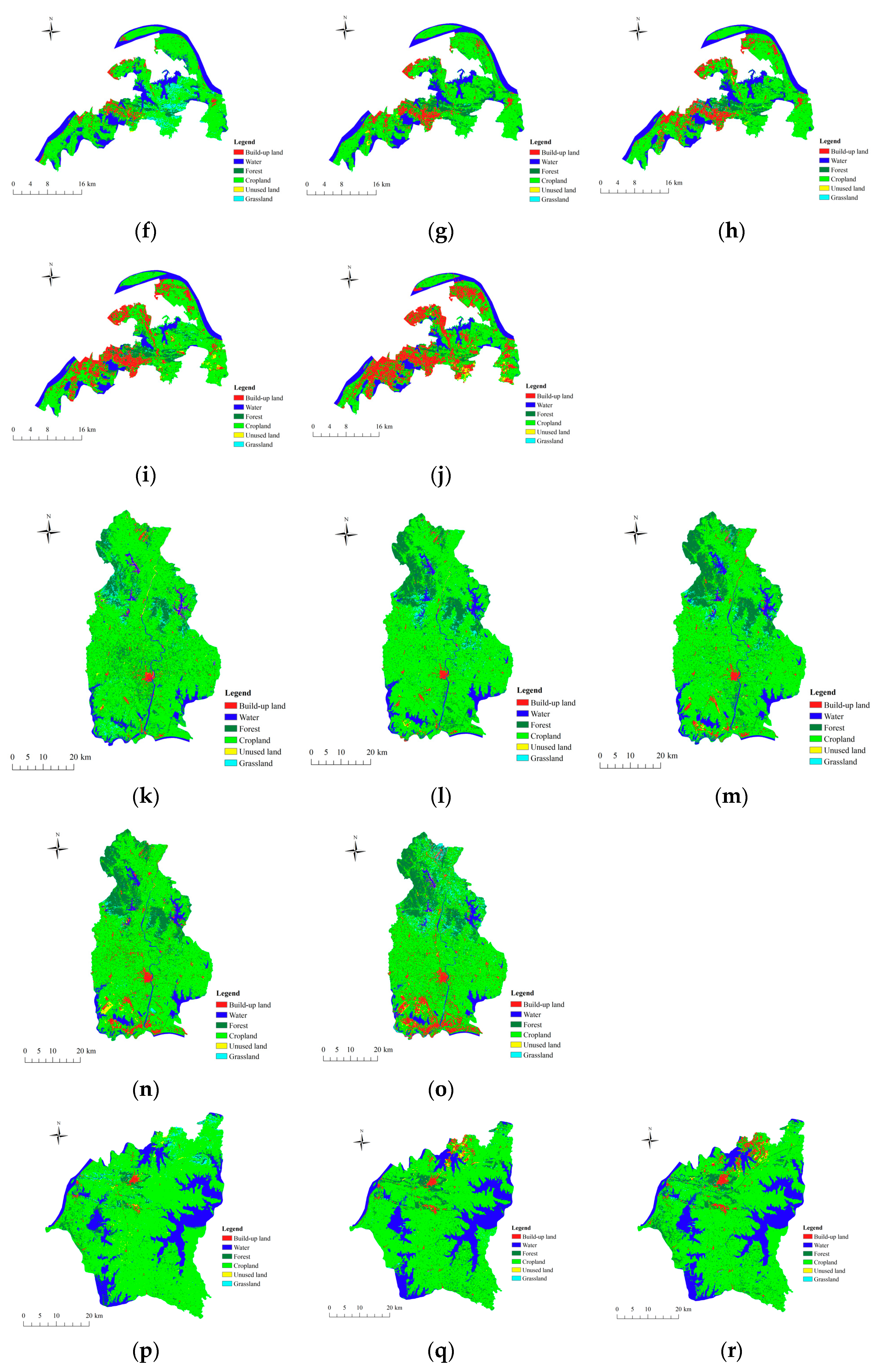
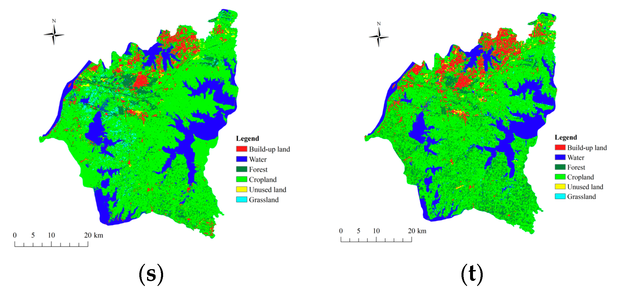
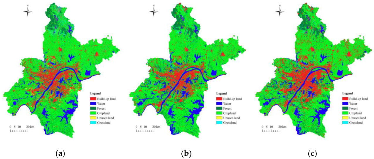
4.1. LULC Maps and Accuracy Assessment
4.2. Temporal Change Analysis by Land Use Theme
4.2.1. Built-Up Land Expansion and Cropland Consumption
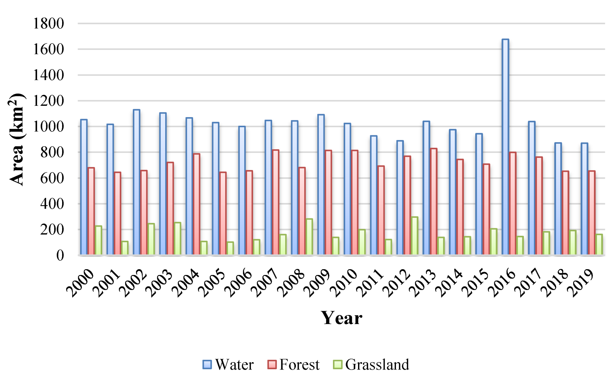
4.2.2. Natural Habitat Dynamics
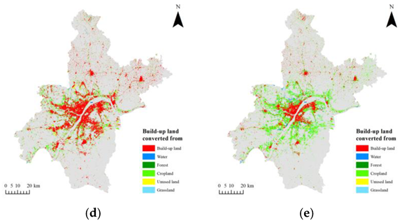
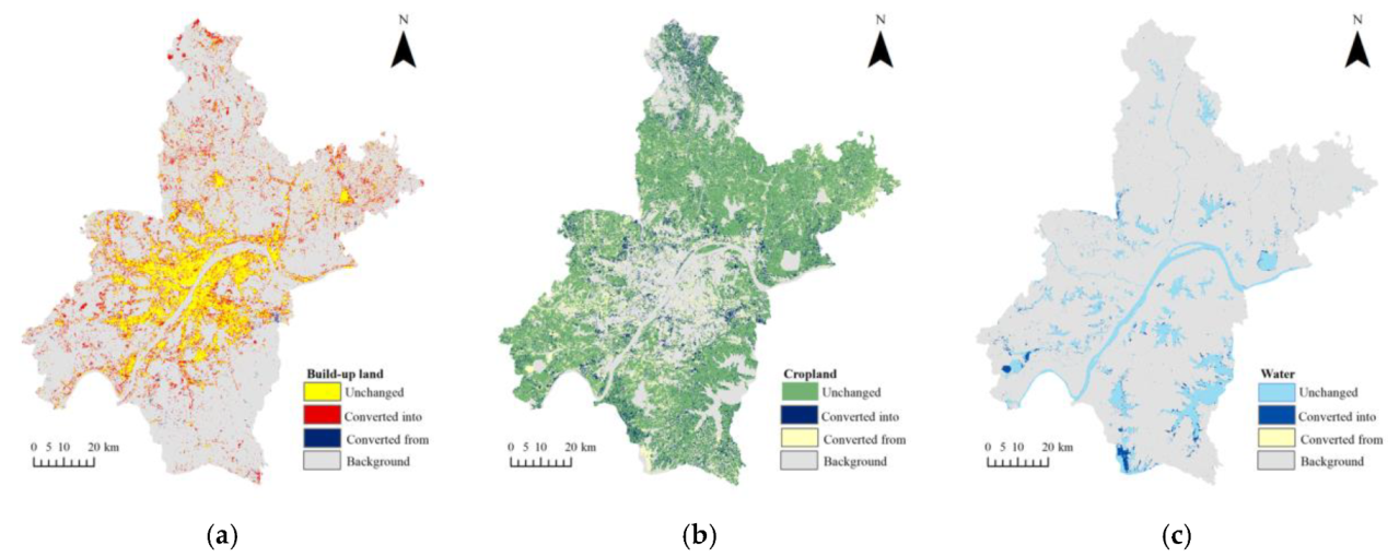
4.2.3. Land Use Conversions
4.3. Spatio-Temporal Pattern Analysis of LULC Change
4.3.1. Single Land Use Dynamicity
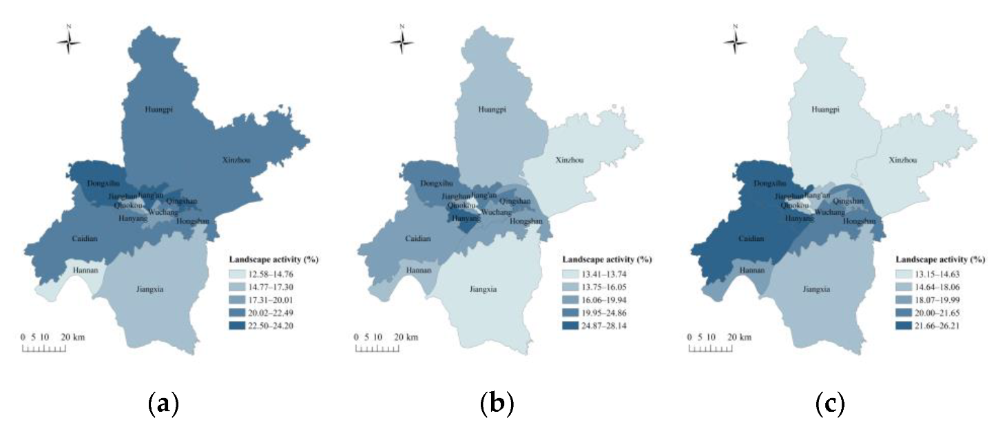
4.3.2. Comprehensive Landscape Activity
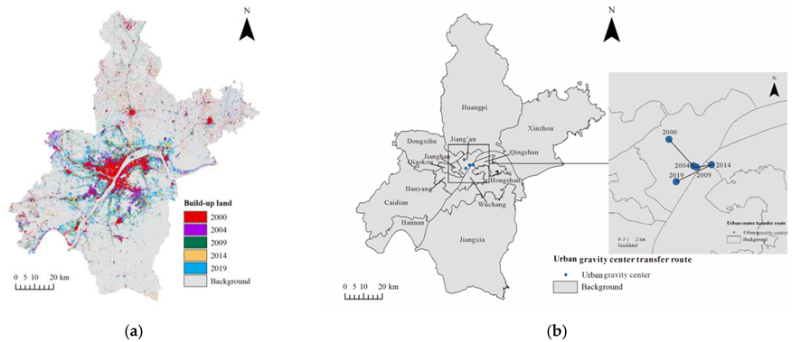
4.3.3. Land Dynamics of Typical Districts
4.3.4. Urbanization Mode and Land Consumption
4.4. Simulated LULC Results
5. Discussion
5.1. Land Use Structure and Dynamicity Analysis
5.1.1. Land Use Structure Characteristics
5.1.2. Land Dynamic Characteristics
5.2. Urbanization Mode Analysis
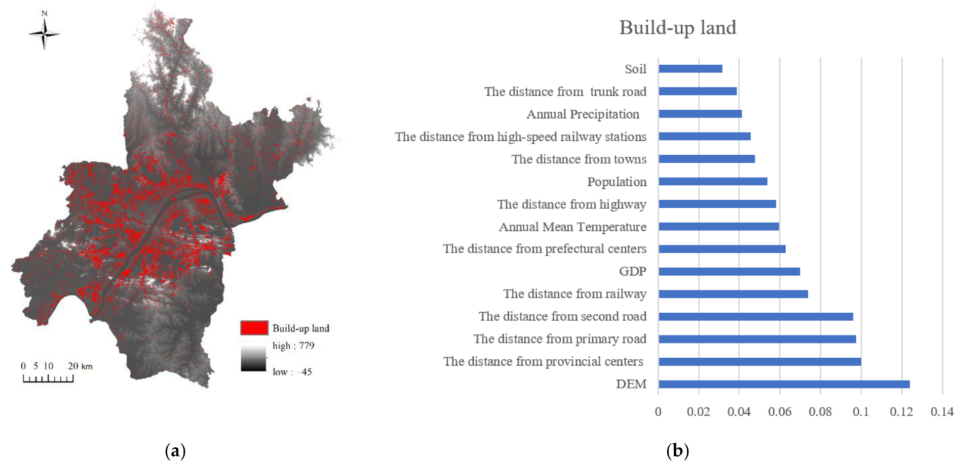
5.2.1. Analysis of Urban Land Crowding out Other Land Uses
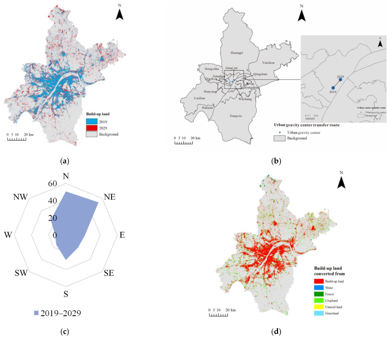
5.2.2. Urban Sprawl Pattern and Gravity Center Transition
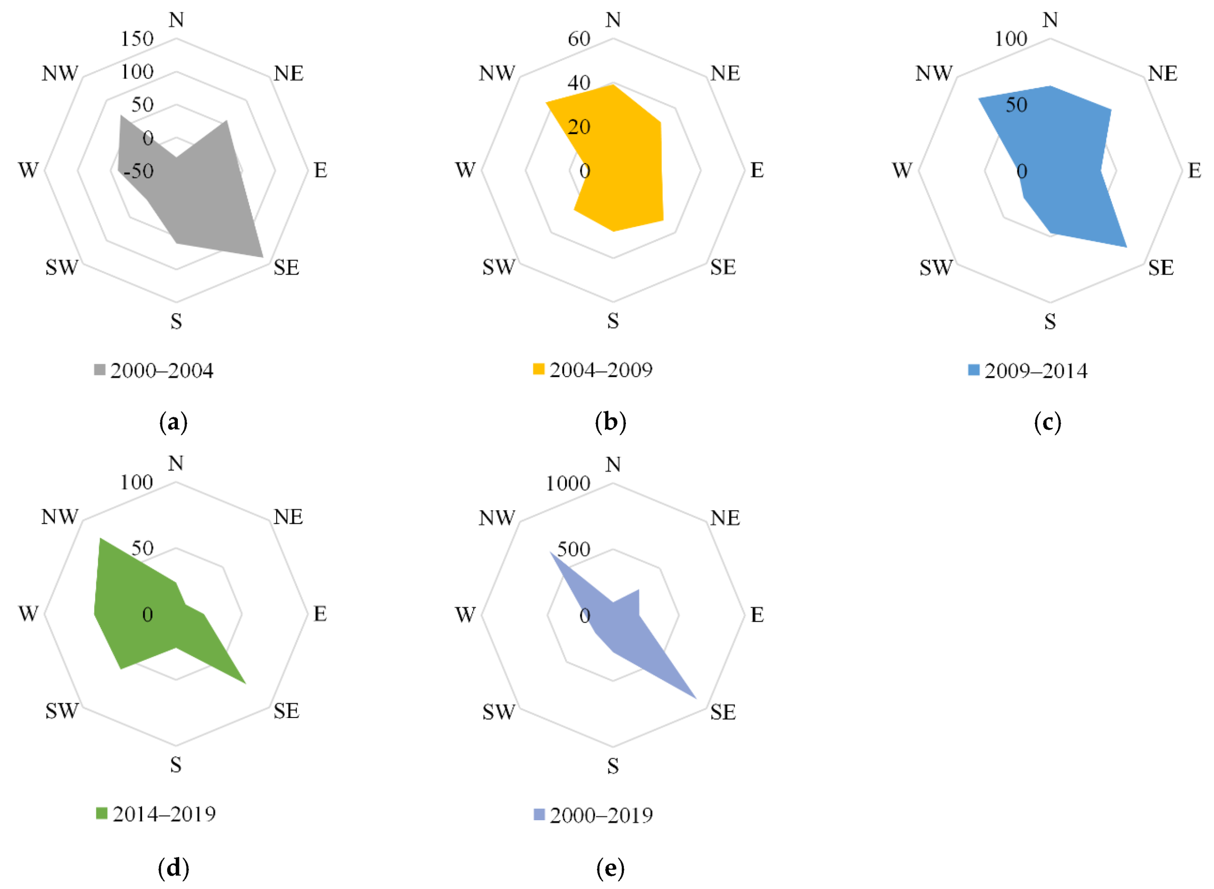
5.2.3. Urban Development Direction
5.3. Future Land Use Dynamic Pattern Analysis
5.3.1. Future Land Use Dynamics
5.3.2. Future Urbanization Mode
6. Conclusions
Author Contributions
Funding
Institutional Review Board Statement
Informed Consent Statement
Data Availability Statement
Acknowledgments
Conflicts of Interest
References
- Sleeter, B.M.; Wilson, T.S.; Sharygin, E.; Sherba, J.T. Future scenarios of land change based on empirical data and demographic trends. Earth’s Future 2017, 5, 1068–1083. [Google Scholar] [CrossRef] [Green Version]
- Homer, C.; Dewitz, J.; Jin, S.; Xian, G.; Costello, C.; Danielson, P.; Gass, L.; Funk, M.; Wickham, J.; Stehman, S.; et al. Conterminous United States land cover change patterns 2001–2016 from the 2016 national land cover database. ISPRS J. Photogramm. Remote Sens. 2020, 162, 184–199. [Google Scholar] [CrossRef]
- Yee, S.H.; Paulukonis, E.; Simmons, C.; Russell, M.; Fulford, R.; Harwell, L.; Smith, L.M. Projecting effects of land use change on human well-being through changes in ecosystem services. Ecol. Model. 2021, 440, 109358. [Google Scholar] [CrossRef] [PubMed]
- Lee, R.J. Vacant land, flood exposure, and urbanization: Examining land cover change in the Dallas-Fort Worth metro area. Landsc. Urban Plan. 2021, 209, 104047. [Google Scholar] [CrossRef]
- Thonfeld, F.; Steinbach, S.; Muro, J.; Hentze, K.; Games, I.; Näschen, K.; Kauzeni, P.F. The impact of anthropogenic land use change on the protected areas of the Kilombero catchment, Tanzania. ISPRS J. Photogramm. Remote Sens. 2020, 168, 41–55. [Google Scholar] [CrossRef]
- Foley, J.A.; DeFries, R.; Asner, G.P.; Barford, C.; Bonan, G.; Carpenter, S.R.; Chapin, F.S.; Coe, M.T.; Daily, G.C.; Gibbs, H.K.; et al. Global consequences of land use. Science 2005, 309, 570–574. [Google Scholar] [CrossRef] [PubMed] [Green Version]
- Zhang, P.; Kohli, D.; Sun, Q.; Zhang, Y.; Liu, S.; Sun, D. Spatial and temporal dimensions of urban expansion in China. Environ. Sci. Technol. 2020, 49, 9600–9609. [Google Scholar]
- Cao, Y.; Kong, L.; Zhang, L.; Ouyang, Z. The balance between economic development and ecosystem service value in the process of land urbanization: A case study of China’s land urbanization from 2000 to 2015. Land Use Policy 2021, 108, 105536. [Google Scholar] [CrossRef]
- Herold, M.; Goldstein, N.C.; Clarke, K.C. The spatiotemporal form of urban growth: Measurement, analysis, and modeling. Remote Sens. Environ. 2003, 86, 286–302. [Google Scholar] [CrossRef]
- Schneider, A.; Friedl, M.A.; Potere, D. A new map of global urban extent from MODIS satellite data. Environ. Res. Lett. 2009, 4, 044003. [Google Scholar] [CrossRef] [Green Version]
- Mertes, C.M.; Schneider, A.; Sulla-Menashe, D.; Tatem, A.J.; Tan, B. Detecting change in urban areas at continental scales with MODIS data. Remote Sens. Environ. 2015, 158, 331–347. [Google Scholar] [CrossRef]
- Yu, W.; Zhou, W.; Jing, C.; Zhang, Y.; Qian, Y. Quantifying highly dynamic urban landscapes: Integrating object-based image analysis with Landsat time series data. Landsc. Ecol. 2021, 36, 1845–1861. [Google Scholar] [CrossRef]
- He, C.; Gao, B.; Huang, Q.; Ma, Q.; Dou, Y. Environmental degradation in the urban areas of China: Evidence from multi-source remote sensing data. Remote Sens. Environ. 2017, 193, 65–75. [Google Scholar] [CrossRef]
- Li, B.; Shi, X.; Lian, L.; Chen, Y.; Chen, Z.; Sun, X. Quantifying the effects of climate variability, direct and indirect land use change, and human activities on runoff. J. Hydrol. 2020, 584, 124684. [Google Scholar] [CrossRef]
- Avashia, V.; Garg, A.; Dholakia, H. Understanding temperature related health risk in context of urban land use changes. Landsc. Urban Plan. 2021, 212, 104107. [Google Scholar] [CrossRef]
- Mwambo, F.M.; Fürst, C.; Nyarko, B.K.; Borgemeister, C.; Martius, C. Maize production and environmental costs: Resource evaluation and strategic land use planning for food security in northern Ghana by means of coupled energy and data envelopment analysis. Land Use Policy 2020, 95, 104490. [Google Scholar] [CrossRef]
- Wan, H.; Shao, Y.; Campbell, J.B.; Deng, X. Mapping annual urban change using time series Landsat and NLCD. Photogramm. Eng. Remote Sens. 2019, 85, 715–724. [Google Scholar] [CrossRef]
- Gala, T.S.; Boakye, L. Spatiotemporal analysis of remotely sensed Landsat time series data for monitoring 32 years of urbanization. J. Hum. Cap. 2020, 5, 85–98. [Google Scholar]
- Seto, K.C.; Fragkias, M. Quantifying spatiotemporal patterns of urban land-use change in four cities of China with time series landscape metrics. Landsc. Ecol. 2005, 20, 871–888. [Google Scholar] [CrossRef]
- Li, X.; Zhou, Y.; Zhu, Z.; Liang, L.; Yu, B.; Cao, W. Mapping annual urban dynamics (1985–2015) using time series of Landsat data. Remote Sens. Environ. 2018, 216, 674–683. [Google Scholar] [CrossRef]
- Zheng, Q.; Weng, Q.; Wang, K. Characterizing urban land changes of 30 global megacities using nighttime light time series stacks. ISPRS J. Photogramm. Remote Sens. 2021, 173, 10–23. [Google Scholar] [CrossRef]
- Bai, X.; Shi, P.; Liu, Y. Realizing China’s urban dream. Nature 2014, 509, 158–160. [Google Scholar] [CrossRef] [Green Version]
- Zhu, S.; Kong, X.; Jiang, P. Identification of the human-land relationship involved in the urbanization of rural settlements in Wuhan city circle, China. J. Rural Stud. 2020, 77, 75–83. [Google Scholar] [CrossRef]
- Huang, X.; Wen, D.; Li, J.; Qin, R. Multi-level monitoring of subtle changes of the megacities of China using high-resolution multi-view satellite imagery. Remote Sens. Environ. 2017, 196, 56–75. [Google Scholar] [CrossRef]
- Zhao, S.; Zhou, D.; Zhu, C.; Sun, Y.; Wu, W.; Liu, S. Remote sensing modeling of urban density dynamics across 36 major cities in China: Fresh insights from hierarchical urbanized space. Landsc. Urban Plan. 2015, 203, 103896. [Google Scholar]
- Gong, P.; Li, X.; Zhang, W. 40-Year (1978–2017) human settlement changes in China reflected by impervious surfaces from satellite remote sensing. Sci. Bull. 2019, 64, 756–763. [Google Scholar] [CrossRef] [Green Version]
- Weng, Q. Land use change analysis in the Zhujiang Delta of China using satellite remote sensing, GIS and stochastic modeling. J. Environ. Manag. 2002, 64, 273–284. [Google Scholar] [CrossRef] [Green Version]
- Yang, C.; Zhang, C.; Li, Q.; Liu, H.; Wu, G. Rapid urbanization and policy variation greatly drive ecological quality evolution in Guangdong-Hong Kong-Macau Greater Bay Area of China: A remote sensing perspective. Ecol. Indic. 2020, 115, 106373. [Google Scholar] [CrossRef]
- Du, J.; Thill, J.C.; Peiser, R.B.; Feng, C. Urban land market and land-use changes in post-reform China: A case study of Beijing. Landsc. Urban Plan. 2014, 124, 118–128. [Google Scholar] [CrossRef]
- Yin, J.; Yin, Z.; Zhong, H.; Xu, S.; Hu, X.; Wang, J.; Wu, J. Monitoring urban expansion and land use/land cover changes of Shanghai metropolitan area during the transitional economy (1979–2009) in China. Environ. Monit. Assess. 2011, 177, 609–621. [Google Scholar] [CrossRef] [PubMed]
- Xiao, J.; Shen, Y.; Ge, J.; Tateishi, R.; Tang, C.; Liang, Y.; Huang, Z. Evaluating urban expansion and land use change in Shijiazhuang, China, by using GIS and remote sensing. Landsc. Urban Plan. 2006, 75, 69–80. [Google Scholar] [CrossRef]
- Kabba, V.; Li, J. Analysis of land use and land cover changes, and their ecological implications in Wuhan, China. J. Geogr. Geol. 2011, 3, 104. [Google Scholar] [CrossRef]
- Li, X.; Ying, W.; Li, J.; Lei, B. Physical and socioeconomic driving forces of land-use and land-cover changes: A case study of Wuhan City, China. Discret. Dyn. Nat. Soc. 2016, 2016, 8061069. [Google Scholar] [CrossRef] [Green Version]
- Liu, Y.; Luo, T.; Liu, Z.; Kong, X.; Li, J.; Tan, R. A comparative analysis of urban and rural construction land use change and driving forces: Implications for urban-rural coordination development in Wuhan, Central China. Habitat Int. 2015, 47, 125–133. [Google Scholar] [CrossRef]
- Ji, C.; Wang, Z.; Zhang, H. Integrated evaluation of coupling coordination for land use change and ecological security: A case study in Wuhan City of Hubei Province, China. Int. J. Environ. Res. Public Health 2017, 62, 236–248. [Google Scholar]
- Liang, X.; Guan, Q.; Clarke, K.C.; Liu, S.; Wang, B.; Yao, Y. Understanding the drivers of sustainable land expansion using a patch-generating land use simulation (PLUS) model: A case study in Wuhan, China. Comput. Environ. Urban Syst. 2021, 85, 101569. [Google Scholar] [CrossRef]
- Che, X.; Zhang, H.; Liu, J. Making Landsat 5, 7 and 8 reflectance consistent using MODIS nadir-BRDF adjusted reflectance as reference. Remote Sens. Environ. 2021, 262, 112517. [Google Scholar] [CrossRef]
- Zhai, H.; Zhang, H.; Zhang, L.; Li, P. Cloud/shadow detection based on spectral indices for multi/hyperspectral optical remote sensing imagery. ISPRS J. Photogramm. Remote Sens. 2018, 144, 235–253. [Google Scholar] [CrossRef]
- Mirchooli, F.; Sadeghi, S.H.; Darvishan, A.K. Analyzing spatial variations of relationships between Land Surface Temperature and some remotely sensed indices in different land uses. Remote Sens. Appl. Soc. Environ. 2020, 19, 100359. [Google Scholar] [CrossRef]
- Feng, Y.; Li, H.; Tong, X.; Chen, L.; Liu, Y. Projection of land surface temperature considering the effects of future land change in the Taihu Lake Basin of China. Glob. Planet. Chang. 2018, 167, 24–34. [Google Scholar] [CrossRef]
- Burges, C.J. A tutorial on support vector machines for pattern recognition. Data Min. Knowl. Discov. 1998, 2, 121–167. [Google Scholar] [CrossRef]
- Oommen, T.; Misra, D.; Twarakavi, N.K.; Prakash, A.; Sahoo, B.; Bandopadhyay, S. An objective analysis of support vector machine based classification for remote sensing. Math. Geosci. 2008, 40, 409–424. [Google Scholar] [CrossRef]
- Pal, M.; Mather, P.M. Support vector machines for classification in remote sensing. Int. J. Remote Sens. 2005, 26, 1007–1011. [Google Scholar] [CrossRef]
- Inglada, J. Automatic recognition of man-made objects in high resolution optical remote sensing images by SVM classification of geometric image features. ISPRS J. Photogramm. Remote Sens. 2007, 62, 236–248. [Google Scholar] [CrossRef]
- Mathur, A.; Foody, G.M. Multiclass and binary SVM classification: Implications for training and classification users. IEEE Geosci. Remote Sens. Lett. 2008, 5, 241–245. [Google Scholar] [CrossRef]
- Liu, S.; Su, H.; Cao, G.; Wang, S.; Guan, Q. Learning from data: A post classification method for annual land cover analysis in urban areas. ISPRS J. Photogramm. Remote Sens. 2019, 154, 202–215. [Google Scholar] [CrossRef]
- Gibson, R.; Danaher, T.; Hehir, W.; Collins, L. A remote sensing approach to mapping fire severity in south-eastern Australia using sentinel 2 and random forest. Remote Sens. Environ. 2020, 240, 111702. [Google Scholar] [CrossRef]
- Bayad, M.; Chau, H.W.; Trolove, S.; Müller, K.; Condron, L.; Moir, J.; Li, Y. Time series of remote sensing and water deficit to predict the occurrence of soil water repellency in New Zealand pastures. ISPRS J. Photogramm. Remote Sens. 2020, 169, 292–300. [Google Scholar] [CrossRef]
- Wu, Q.; Zhang, S.; Zhao, Z. Research on multi-level urban development trend based on spatio-temporal analysis. Geospat. Inf. 2021, 19, 14–16. [Google Scholar]
- Chen, Y.; Li, X.; Liu, X.; Ai, B. Modeling urban land-use dynamics in a fast developing city using the modified logistic cellular automaton with a patch-based simulation strategy. Int. J. Geogr. Inf. Sci. 2013, 28, 234–255. [Google Scholar] [CrossRef]
- Gounaridis, D.; Chorianopoulos, I.; Symeonakis, E.; Koukoulas, S. A random Forest-cellular automata modelling approach to explore future land use/cover change in Attica (Greece), under different socio-economic realities and scales. Sci. Total Environ. 2019, 646, 320–335. [Google Scholar] [CrossRef] [PubMed]
- Lucas, I.F.; Frans, J.M.; Wel, V.D. Accuracy assessment of satellite derived land-cover data: A review. Photogramm. Eng. Remote Sens. 1994, 60, 410–432. [Google Scholar]


| Year | Sensor | Acquisition Date (/Month-Day/) (Path/Row: 122/39, 123/38, 123/39) | Utilized Bands |
|---|---|---|---|
| 2000 | Landsat 5 TM | 9-22/9-13/9-13 | B/G/R/NIR/SWIR-I/SWIR-II |
| 2001 | Landsat5 TM | 7-10/9-3/9-3 | B/G/R/NIR/SWIR-I/SWIR-II |
| 2002 | Landsat5 TM | 5-26/5-1/5-1 | B/G/R/NIR/SWIR-I/SWIR-II |
| 2003 | Landsat5 TM | 9-17/9-24/9-24 | B/G/R/NIR/SWIR-I/SWIR-II |
| 2004 | Landsat 5 TM | 7-18/9-11/9-11 | B/G/R/NIR/SWIR-I/SWIR-II |
| 2005 | Landsat5 TM | 6-19/4-7/4-7 | B/G/R/NIR/SWIR-I/SWIR-II |
| 2006 | Landsat5 TM | 7-8/7-31/7-31 | B/G/R/NIR/SWIR-I/SWIR-II |
| 2007 | Landsat5 TM | 3-4/4-28/4-28 | B/G/R/NIR/SWIR-I/SWIR-II |
| 2008 | Landsat5 TM | 7-13/9-6/9-6 | B/G/R/NIR/SWIR-I/SWIR-II |
| 2009 | Landsat5 TM | 11-5/11-12/11-12 | B/G/R/NIR/SWIR-I/SWIR-II |
| 2010 | Landsat5 TM | 8-20/6-8/6-8 | B/G/R/NIR/SWIR-I/SWIR-II |
| 2011 | Landsat5 TM | 5-10/5-17/5-17 | B/G/R/NIR/SWIR-I/SWIR-II |
| 2012 | Landsat7 ETM+ | 8-9/9-17/9-17 | B/G/R/NIR/SWIR-I/SWIR-II |
| 2013 | Landsat8 OLI | 10-15/10-6/10-6 | C/B/G/R/NIR/SWIR-I/SWIR-II |
| 2014 | Landsat8 OLI | 9-22/9-13/9-13 | C/B/G/R/NIR/SWIR-I/SWIR-II |
| 2015 | Landsat8 OLI | 10-18/10-25/10-25 | C/B/G/R/NIR/SWIR-I/SWIR-II |
| 2016 | Landsat8 OLI | 8-1/7-23/7-23 | C/B/G/R/NIR/SWIR-I/SWIR-II |
| 2017 | Landsat8 OLI | 4-30/7-26/8-27 | C/B/G/R/NIR/SWIR-I/SWIR-II |
| 2018 | Landsat8 OLI | 4-17/4-8/4-8 | C/B/G/R/NIR/SWIR-I/SWIR-II |
| 2019 | Landsat5 TM | 8-18/8-25/8-25 | C/B/G/R/NIR/SWIR-I/SWIR-II |
| Category | Data | Original Resolution | Data Resource |
|---|---|---|---|
| Socioeconomic driving factors | Population | 1000 m | http://www.geodoi.ac.cn/WebCn/Default.aspx (accessed on 3 March 2021) |
| GDP | |||
| The distance from highway | 30 m | OpenStreetMap (https://www.openstreetmap.org/) (accessed on 3 March 2021) | |
| The distance from railway | |||
| The distance from trunk road | |||
| The distance from primary road | |||
| The distance from second road | |||
| The distance from high-speed railway stations | |||
| The distance from provincial centers | |||
| The distance from prefectural centers | |||
| The distance from towns | |||
| Natural driving factors | Soil | 1000 m | HWSD v1.2 (http://westdc.westgis.ac.cn/data/844010ba-d359-4020-bf76-2b58806f9205) (accessed on 4 March 2021) |
| DEM | 30 m | NASA SRTM1 v3.0 | |
| Annual mean temperature | 1000 m | WorldClim v2.0 (http://www.worldclim.org/) (accessed on 4 March 2021) | |
| Annual precipitation |
| Year | Original Classification | Temporal Consistency | Spatial Coherence | |||
|---|---|---|---|---|---|---|
| OA (%) | Kappa | OA (%) | Kappa | OA (%) | Kappa | |
| 2000 | 86.17% | 0.8218 | 86.17% | 0.8218 | 88.31% | 0.8490 |
| 2001 | 79.94% | 0.7415 | 82.97% | 0.7789 | 84.86% | 0.8032 |
| 2002 | 86.96% | 0.8318 | 88.19% | 0.8469 | 89.54% | 0.8641 |
| 2003 | 85.25% | 0.8142 | 86.19% | 0.8250 | 87.86% | 0.8459 |
| 2004 | 84.31% | 0.7938 | 86.85% | 0.8250 | 89.04% | 0.8539 |
| 2005 | 90.36% | 0.8687 | 91.27% | 0.8806 | 92.87% | 0.9022 |
| 2006 | 87.61% | 0.8368 | 89.89% | 0.8663 | 91.58% | 0.8885 |
| 2007 | 89.11% | 0.8561 | 90.46% | 0.8731 | 91.91% | 0.8923 |
| 2008 | 87.44% | 0.8354 | 88.76% | 0.8520 | 90.49% | 0.8744 |
| 2009 | 87.66% | 0.8369 | 88.23% | 0.8438 | 89.66% | 0.8626 |
| 2010 | 82.88% | 0.7763 | 82.88% | 0.7763 | 85.52% | 0.8098 |
| 2011 | 84.09% | 0.7943 | 83.61% | 0.7877 | 85.77% | 0.8153 |
| 2012 | 88.56% | 0.8530 | 88.56% | 0.8530 | 89.44% | 0.8638 |
| 2013 | 85.58% | 0.8122 | 86.50% | 0.8229 | 88.04% | 0.8427 |
| 2014 | 89.27% | 0.8611 | 90.21% | 0.8727 | 91.66% | 0.8913 |
| 2015 | 88.40% | 0.8510 | 87.54% | 0.8384 | 89.27% | 0.8606 |
| 2016 | 87.02% | 0.8261 | 87.02% | 0.8261 | 88.46% | 0.8449 |
| 2017 | 84.67% | 0.8001 | 84.67% | 0.8001 | 86.56% | 0.8244 |
| 2018 | 87.09% | 0.8247 | 86.73% | 0.8194 | 88.45% | 0.8425 |
| 2019 | 89.60% | 0.8632 | 89.60% | 0.8632 | 91.09% | 0.8826 |
| 2019 | Built-Up Land | Water | Forest | Cropland | Unused Land | Grassland | |
|---|---|---|---|---|---|---|---|
| 2000 | |||||||
| Built-up land | 305.08 | 7.73 | 5.46 | 99.05 | 4.83 | 8.40 | |
| Water | 55.13 | 707.46 | 20.92 | 248.92 | 1.92 | 17.94 | |
| Forest | 42.13 | 42.75 | 229.46 | 348.52 | 4.61 | 10.74 | |
| Cropland | 947.37 | 103.45 | 349.69 | 4463.39 | 100.04 | 113.86 | |
| Unused land | 34.77 | 7.64 | 4.24 | 61.10 | 5.42 | 2.54 | |
| Grassland | 28.72 | 0.97 | 44.57 | 139.74 | 4.82 | 7.14 | |
| Land Use Dynamicity (%) | 2000–2004 | 2004–2009 | 2009–2014 | 2014–2019 | 2000–2019 |
|---|---|---|---|---|---|
| Built-up land | 7.01 | 5.15 | 9.09 | 8.03 | 12.01 |
| Cropland | −0.28 | −0.71 | −0.66 | −0.87 | −0.62 |
| Water | 0.34 | 0.44 | −2.12 | −2.16 | −0.91 |
| Forest | 4.03 | 0.66 | −1.70 | −2.42 | −0.19 |
| Grassland | −13.20 | 5.84 | 0.81 | 2.45 | −1.51 |
| Unused land | −12.12 | −2.83 | 21.29 | 3.02 | 0.27 |
| Period | 2000–2004 | 2004–2009 | 2009–2014 | 2014–2019 |
|---|---|---|---|---|
| Transition distance (km) | 4.10 | 0.38 | 1.73 | 4.46 |
Publisher’s Note: MDPI stays neutral with regard to jurisdictional claims in published maps and institutional affiliations. |
© 2021 by the authors. Licensee MDPI, Basel, Switzerland. This article is an open access article distributed under the terms and conditions of the Creative Commons Attribution (CC BY) license (https://creativecommons.org/licenses/by/4.0/).
Share and Cite
Zhai, H.; Lv, C.; Liu, W.; Yang, C.; Fan, D.; Wang, Z.; Guan, Q. Understanding Spatio-Temporal Patterns of Land Use/Land Cover Change under Urbanization in Wuhan, China, 2000–2019. Remote Sens. 2021, 13, 3331. https://0-doi-org.brum.beds.ac.uk/10.3390/rs13163331
Zhai H, Lv C, Liu W, Yang C, Fan D, Wang Z, Guan Q. Understanding Spatio-Temporal Patterns of Land Use/Land Cover Change under Urbanization in Wuhan, China, 2000–2019. Remote Sensing. 2021; 13(16):3331. https://0-doi-org.brum.beds.ac.uk/10.3390/rs13163331
Chicago/Turabian StyleZhai, Han, Chaoqun Lv, Wanzeng Liu, Chao Yang, Dasheng Fan, Zikun Wang, and Qingfeng Guan. 2021. "Understanding Spatio-Temporal Patterns of Land Use/Land Cover Change under Urbanization in Wuhan, China, 2000–2019" Remote Sensing 13, no. 16: 3331. https://0-doi-org.brum.beds.ac.uk/10.3390/rs13163331