
Interseismic Slip and Coupling along the Haiyuan Fault Zone Constrained by InSAR and GPS Measurements


1
State Key Laboratory of Earthquake Dynamics, Institute of Geology, China Earthquake Administration, Beijing 100029, China
2
Guangdong Provincial Key Laboratory of Geodynamics and Geohazards, School of Earth Sciences and Engineering, Sun Yat-Sen University, Zhuhai 519000, China
*
Author to whom correspondence should be addressed.
Remote Sens. 2021, 13(16), 3333; https://0-doi-org.brum.beds.ac.uk/10.3390/rs13163333
Submission received: 29 June 2021
/
Revised: 12 August 2021
/
Accepted: 18 August 2021
/
Published: 23 August 2021
Abstract
:The Haiyuan fault zone is an important tectonic boundary and strong seismic activity belt in northeastern Tibet, but no major earthquake has occurred in the past ∼100 years, since the Haiyuan M8.5 event in 1920. The current state of strain accumulation and seismic potential along the fault zone have attracted significant attention. In this study, we obtained the interseismic deformation field along the Haiyuan fault zone using Envisat/ASAR data in the period 2003–2010, and inverted fault kinematic parameters including the long-term slip rate, locking degree and slip deficit distribution based on InSAR and GPS individually and jointly. The results show that there is near-surface creep in the Laohushan segment of about 19 km. The locking degree changes significantly along the strike with the western part reaching 17 km and the eastern part of 3–7 km. The long-term slip rate gradually decreases from west 4.7 mm/yr to east 2.0 mm/yr. As such, there is large strain accumulation along the western part of the fault and shallow creep along the Laohushan segment; while in the eastern section, the degree of strain accumulation is low, which suggests the rupture segments of the 1920 earthquake may have been not completely relocked.
1. Introduction
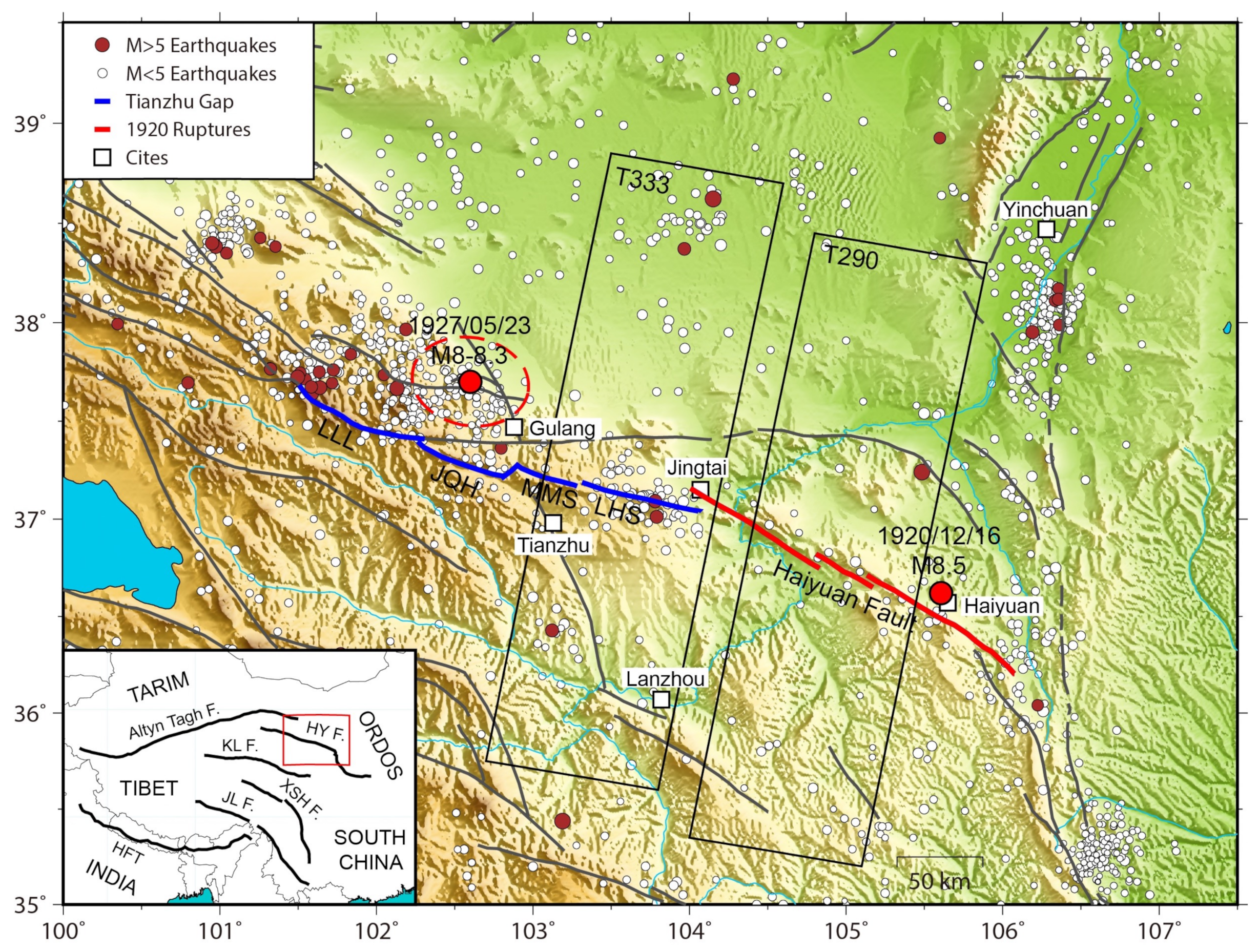
Located on the northeastern margin of the Qinghai-Tibet Plateau, the Haiyuan fault zone is a boundary fault of the stable Alaxan block, the stable Ordos block, and active Tibet (Figure 1); it is the most significant regional fault zone for tectonic deformation and strong earthquake activity. The fault zone is characterised by large left-lateral strike-slip and is bounded by the Liupanshan fault to the east and the northern margin fault of the Qilian Mountains to the west. It consists of several segments, including (from west to east) the Lenglongling (LLL), Jinqianghe (JQH), Maomaoshan (MMS), Laohushan (LHS) segments and the segment of 1920 Haiyuan earthquake rupture. The 1920 M8.5 Haiyuan earthquake resulted in a surface rupture zone of ∼240 km in length, with a maximum left-lateral coseismic displacement of 10 m [1,2]. Since 1920, there have been no destructive earthquakes of M6 or above along the Haiyuan fault; however, it remains unclear whether the fault is in a locked state with accumulating interseismic strain, or in the postseismic adjustment stage. Resolving this uncertainty is important for assessing future seismic hazard along the fault zone.
To investigate the locking degree and future seismic hazard of the Haiyuan fault zone, numerous studies have employed geological and GPS geodetic techniques. The slip rate obtained based on fault geomorphic features and geological dating gradually decreases from west to east. The slip rate of the LLL segment is 19 ± 5 mm/yr during the Postglacial period [3], and that of the LHS and MMS segments is 12 ± 4 mm/yr and just 3.5–10 mm/yr at the 1920 rupture segment (4.5 ± 1.0 mm/yr (Late Quaternary) [4]; 8 ± 2 mm/yr (Holocene epoch) [5]; 5–10 mm/yr (After the end of the Pliocene time) [6]). However, Ref. [7] derived a late Quaternary slip rate of only 4–5 mm/yr from the LLL segment to the middle of the 1920 rupture, and 1–3 mm/yr or lower along the easternmost end of the fault zone. The geological approach is traditionally used for fault activity research; however, dislocation measurements can only be performed on good local fault outcrops. In the Haiyuan fault zone, there are a limited number of field measurement points and observations are not equally distributed owing to the sampling locations and sampling method. To address this issue, GPS geodetic technology can be used to investigate the deformation of active blocks and fault zones.
Many studies have used GPS data to obtain the strike-slip rate of the Haiyuan fault zone, with values ranging from 0.0 to 8.6 mm/yr based on the block model or dislocation model (e.g., 8.6 mm/yr [8]; 5–6 mm/yr [9]; 0.0–4.5 mm/yr [10]; 3.5–6.5 mm/yr [11]. Although there may be a certain difference between the geodetic rate and the long-term geological rate in some areas [12,13], as far as Haiyuan is concerned, they show a good agreement. This may indicate that the interseismic slip rate of Haiyuan has remained relatively stable over a long time scale. This relatively stable rate has also appeared in other areas of the Qinghai-Tibet Plateau, such as the Altyn Tagh fault and the Xianshuihe fault [14,15]. Based on the block model, Refs. [16,17] obtained the locking degree and slip rate deficit distribution of the Haiyuan fault zone; however, the GPS station distribution in the region is sparse, especially near the fault where there is almost no GPS data. Therefore, the spatial resolutions of the locking degree and slip rate deficit estimates obtained using GPS are low and cannot reflect fine-scale variations along the fault.
In recent years, the application of InSAR technology for the observation of interseismic deformation has rapidly developed [18,19,20]. Owing to its high resolution, InSAR can distinguish subtle deformation differences in near-field fault regions or along strike directions; this allows us to perform fine quantitative analyses of slip rate and activity states for different segments. Owing to their complementary advantages, the combination of high-density InSAR data and large-scale sparse GPS can provide good constraints on the active states of far- and near-field regions of an entire fault zone; from this, it is possible to obtain continuous distributions of kinematic parameters along the strike.
At present, a few studies have used InSAR to investigate the Haiyuan fault zone. However, there are few studies on inversion of Haiyuan fault motion parameters by combining high-density InSAR and large-scale GPS data with complementary advantages. Using European remote sensing (ERS) radar data for 1993–1998, Ref. [21] obtained a slip rate of 4.2–8.0 mm/yr along the MMS-LHS segment and found that the eastern LHS segment is in a state of creep, but there is no article pointing out fieldwork evidence of surface creeping until now. Based on 2003–2009 Envisat radar data, Refs. [22,23] estimated an average creep rate of 5.0 mm/yr, which is consistent with the long-term deep loading rate; the local maximum rate was found to be 8.0 mm/yr, which is a transient accelerated creep event and may be triggered by the 2000 5.6 earthquake. Therefore, it is considered that there is no strain accumulation along this segment. The inversion results obtained by [22] based on the Okada model show that there is creep along the LHS segment, while both the Tianzhu seismic gap and the 1920 rupture segment are locked. A left-lateral strike-slip rate of 6.9–10.0 mm/yr along the JQH segment and 4.5–6.9 mm/yr along the MMS segment was estimated by [24] from Envisat data. However, these studies only use InSAR observations and lack constraints of GPS data.
To address the lack of in-depth quantitative research on the activities and coupling states of different segments of the Haiyuan fault zone, we used a combination of InSAR and GPS data to construct an optimized model that considers the fault geometry. In this study, we used Envisat advanced synthetic aperture radar (ASAR) long-strip data from two descending tracks to obtain the average deformation rate field of the Haiyuan fault zone in 2003–2010. We then transformed the deformation rate from the line-of-sight (LOS) direction to the fault parallel direction. A screw dislocation model was used to fit the cross-fault deformation rate profiles, and parameters, such as the fault slip rate and locking depth along the profiles were obtained. We then used a three-dimensional block model to invert the distribution characteristics of the fault locking degree and slip rate deficit in the Haiyuan fault zone. We comparatively analysed the inversion results and differences when using large-scale sparse GPS data alone and in combination with high-density InSAR deformation field, and we obtained a continuous distribution of the strain accumulation state along the fault. The results of this study provide constraints for the prediction of potential earthquake risk along the Haiyuan fault zone and contribute to our understanding of the deformation mechanism of the Qinghai-Tibet Plateau.
2. Interseismic Deformation
2.1. Data and Processing Method
Differential InSAR (DInSAR) technology has been widely used in monitoring deformation fields, such as coseismic deformation, landslides, and glacial movement. However, owing to the influence of orbital error, atmospheric delay, temporal-spatial incoherence, and external digital elevation model (DEM) error, there are certain limitations in measuring small-scale deformation of the Earth’s surface. Time series InSAR analysis addresses the various precision constraints of traditional DInSAR technology processing. By analysing the time series of a large number of SAR images accumulated in a deformation region over many years, the method can effectively separate the micro-deformation phase from the error phases of the orbit and atmosphere, so as to achieve high-precision measurements of crustal deformation. Time series InSAR technologies mainly include the stacking method, persistent scatterers (PS), and small baseline subset algorithm [18,25].
The PSInSAR technique is based on PS and was first proposed by [19,25]. PS are targets with relatively stable scattering characteristics such as artificial buildings and bare rocks. They can generate strong radar echo signals with high signal-to-noise ratios and high phase stability in SAR images over a long period of time. Stanford Method for Persistent Scatterers (StaMPS) is a software package that integrates the PS method into the SBAS method [26,27]; it combines amplitude and phase information to identify PS points and does not require prior knowledge of surface deformation. The StaMPS method takes into account both temporal and spatial baselines, constructs an interference pair network according to the short baseline principle, generates interferograms by registration, removes the flat Earth effect, and uses a DEM to eliminate the influence of the terrain phase. Based on the phase stability characteristics of the PS point, the PS candidate point is selected using the amplitude dispersion threshold; the amplitude deviation value is represented by:
where and are the standard deviation and mean of a series of amplitude values, respectively. For an interferogram that removes the flat Earth effect and the terrain phase, the wrapped phase can be expressed by
where is the phase change caused by the motion of the pixel in the satellite LOS direction, is the atmospheric delay phase difference, is the orbital error, is the look angle error, and is noise. After acquiring PS candidate points, the phase residual of each point is iteratively calculated as:
where N is the number of interferograms, , is the estimate of the spatially correlated part of , and is the estimate of spatially uncorrelated look angle error. The root mean square (RMS) of all candidate points is calculated after each iteration, and points that fluctuate significantly are removed. Iterative convergence is considered when the change in phase residual is less than a certain threshold. When PS points are sufficiently dense, the absolute phase difference of most adjacent points is less than , and phase unwrapping is performed. The unwrapped phase contains spatially correlated errors and non-spatial related errors; the latter can be treated as noise in subsequent processing, while the former can be divided into time-correlated and uncorrelated parts. For the time-correlated part, time domain low pass filtering is used for removal. The spatially correlated and time-uncorrelated part is first processed by time-domain high-pass filtering, and then spatially low-pass filtered for each interferogram [27].
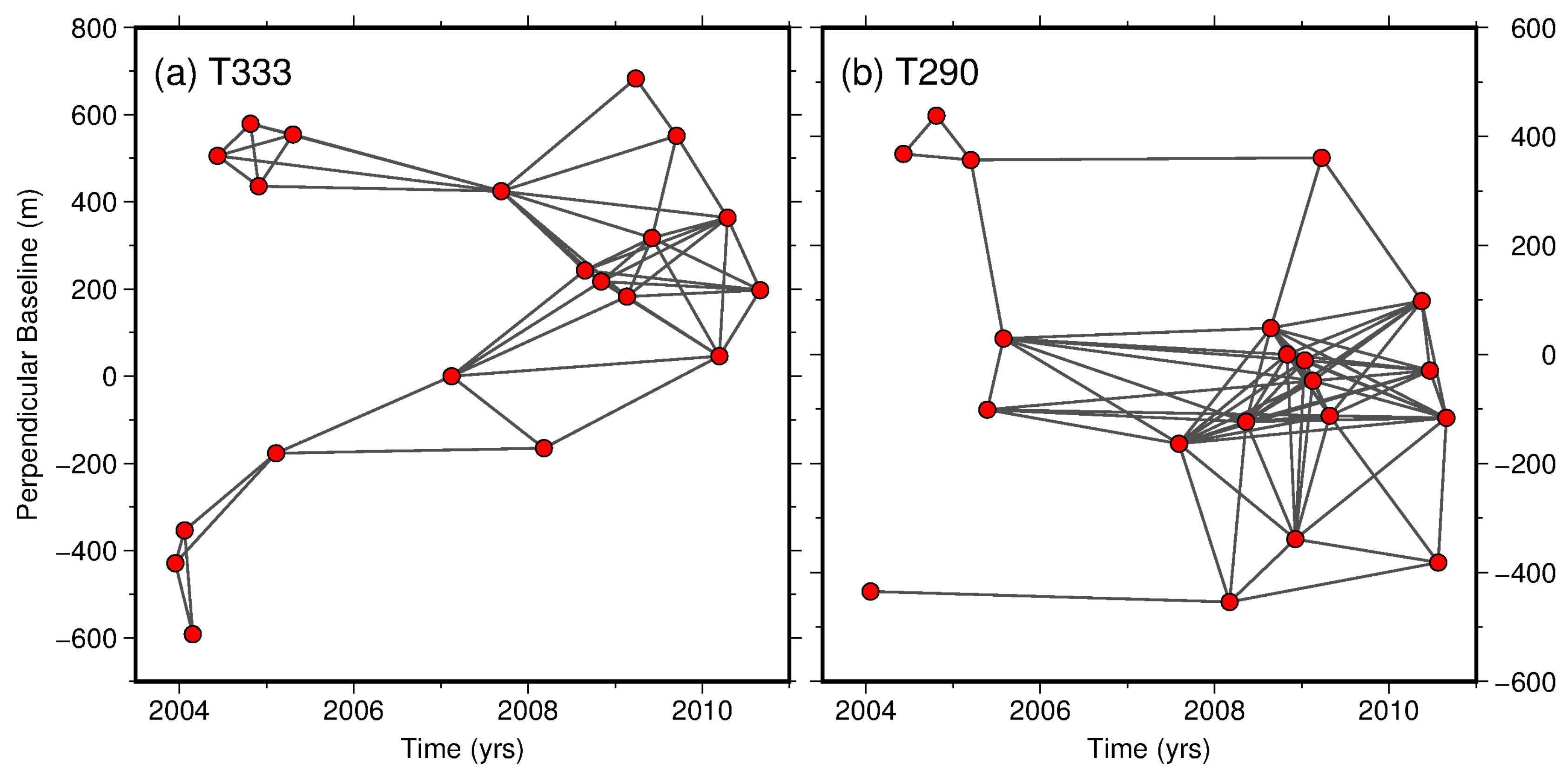
To obtain the interseismic deformation rate field of the Haiyuan fault zone, we processed the Envisat satellite data from two descending tracks. This dataset covers the MMS segment to the middle part of the 1920 rupture for the 2003–2010 period. The temporal-spatial baseline networks of both tracks are shown in Figure 2. To ensure the coherence of the interferograms, the spatial perpendicular baseline of each selected image pair is less than 350 m.
Based on the StaMPS algorithm flow, we used the ROI_PAC software to convert the raw data from RAW format to SLC format. We used the DORIS software to achieve image registration and generate interferograms by image resampling. To remove the effects of the terrain phase we used shuttle radar topography mission (SRTM) 90 m resolution DEM data. Stable PS points were selected based on the amplitude and phase information of pixels; the amplitude deviation was set to 0.4 and the spatially uncorrelated look angle error was estimated and removed. Phase unwrapping was performed using the SNAPHU software. Finally, low-pass filtering was performed spatially, and then high-pass filtering was performed in the time dimension to remove residual atmospheric and orbit errors. When the StaMPS software corrects the orbital ramp, it assumes that there is no bilinear deformation in analysis area. However, the Haiyuan fault is dominated by left-lateral strike-slip and has obvious bilinear deformation in the north and south plates. To address this problem, when correcting the orbital ramp we only used the south plate of the Haiyuan fault zone [15], which had good overall coherence, to fit the orbital ramp and remove it from the whole area.
2.2. InSAR Deformation Rate Field Analysis
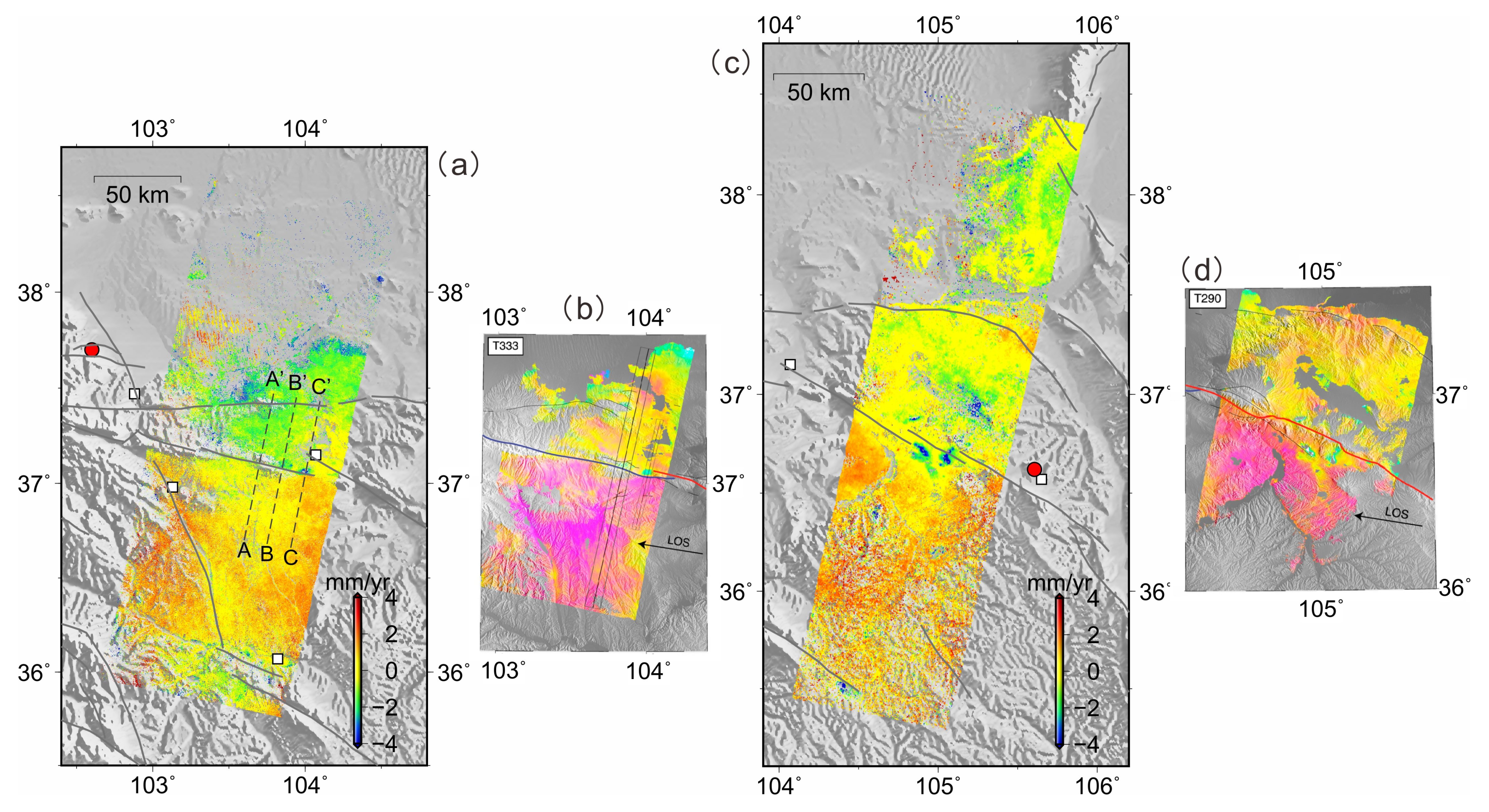
Figure 3 shows the average deformation rate field of the Haiyuan fault zone obtained by each track and covering the area from the MMS segment to the middle of the 1920 rupture; the field also includes the Gulang fault to the north, the Xiangshan–Tianjingshan fault, and other areas. The overall image coherence is good and most of the region has a continuous deformation point distribution. Only the coherence of the north desert area is poor; in this area, there are fewer deformation points and the error is larger. Both tracks show obvious deformation rate differences near the Haiyuan fault. The velocities are positive on the south wall of the fault as a whole, indicating that the south wall moved toward the satellite; on the north side the velocities are 0 or negative, indicating movement away from the satellite. This distribution state is consistent with the left-lateral strike-slip motion of the Haiyuan fault zone. At the same time, we also identified several significant local deformation regions in the velocity field, which was caused by coal mining proved in our field investigation.
2.3. Deformation Profile Fitting Using the Screw Dislocation Model
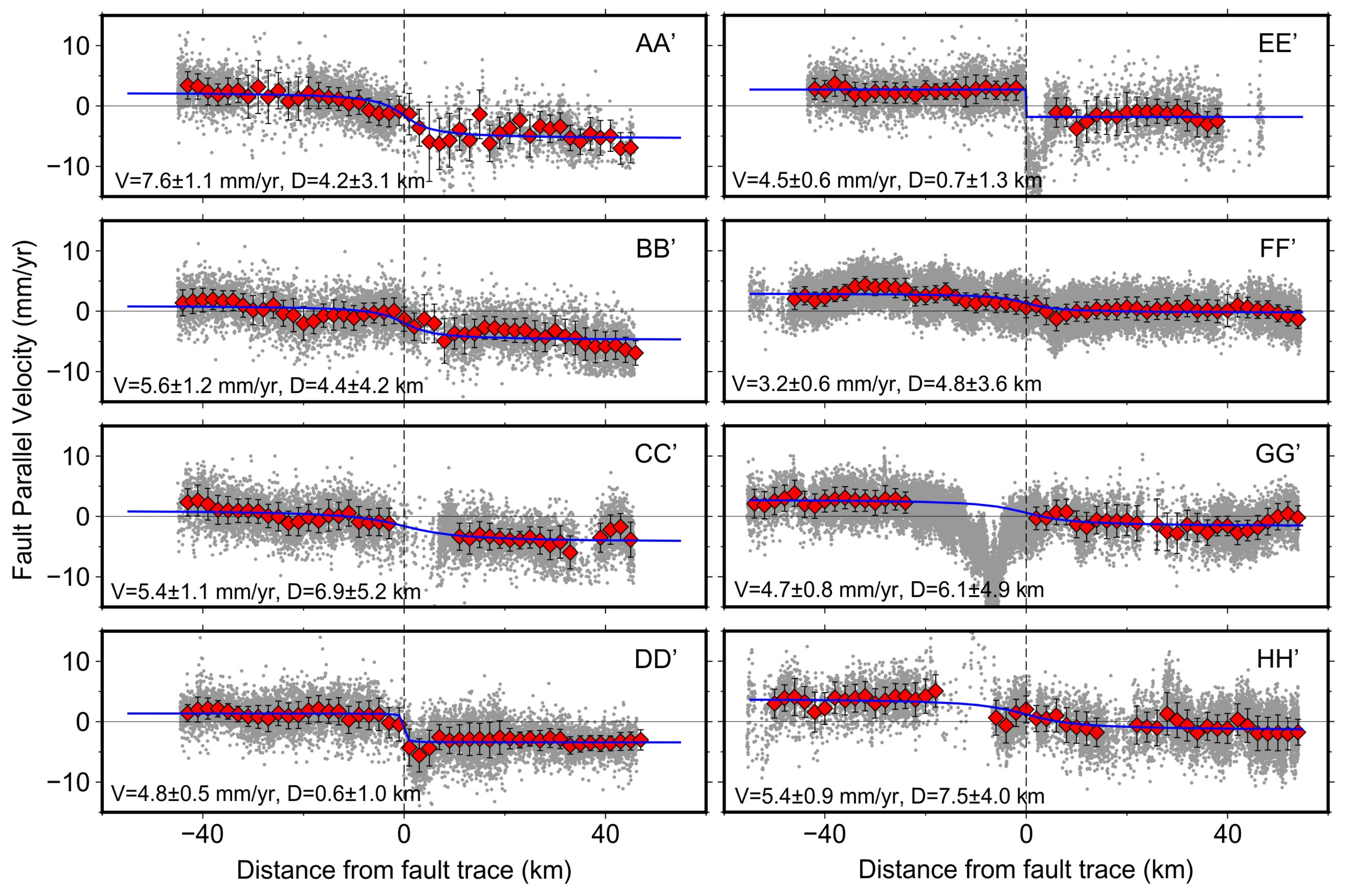
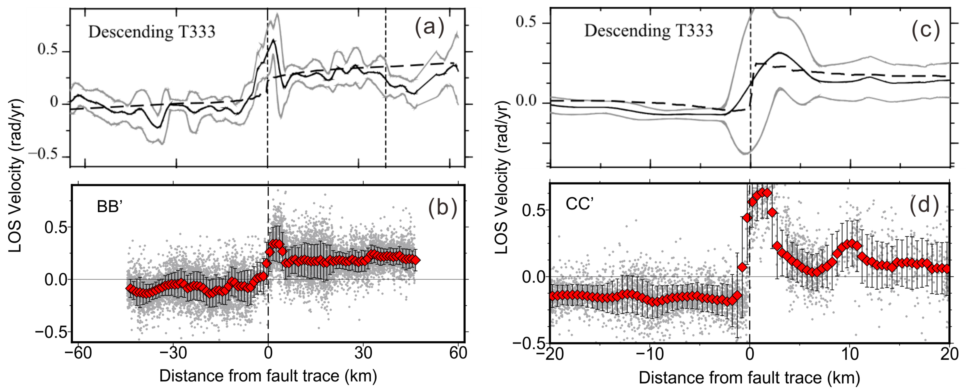
A total of eight rate profiles perpendicular to the fault strike (AA’–HH’ in Figure 3) were drawn across the two tracks, each with a width of 2 km. Existing geological studies [1,6] and GPS observations [8,28] indicate that the Haiyuan fault exhibits left-lateral strike-slip movement. Its motion is dominated by horizontal displacement along the fault; vertical deformation is minor. At the same time, the Haiyuan fault is oriented in a near east–west direction, and the angle between the projection of the satellite observation direction on the horizontal plane and the fault strike is small. Therefore, InSAR is sensitive to strike-slip deformation along the Haiyuan fault. On this basis, we ignored the vertical deformation and assumed that the observed LOS deformation is caused by horizontal deformation along the fault. Then, based on the geometric relationship between the LOS deformation observed by InSAR and the three components of the surface movement, the LOS rate of deformation was translated directly into the horizontal rate along the fault (Figure 4). Considering the stability of the crustal deformation of the fault zone and avoiding the influence of the local velocity steep point on the fitting results, we smoothed the deformation rate profile and calculated the deformation rate average and 1- value according to the 2-km length windows along the profiles. Obvious settlement area along the profiles were masked, and the result are shown by red diamonds in Figure 4. Based on the screw dislocation model [29], we estimated the slip rate and locking depth of different segments of Haiyuan fault; the model expression is as follows:
where is the fault-parallel velocity of the fault with a distance of x to it, is the deep slip rate, x is the distance between the ground observation point and the fault, D is the fault locking depth, and is the rate offset constant. To solve the uncertainty of the average values, we used the Monte Carlo method in the fitting process. In each Monte Carlo simulation, each fault-parallel rate was chosen to be a random value within a 1- error range obeying a normal distribution.
The best fitting results (blue curve in Figure 4) indicate that the slip rate and locking depth of the LHS segment (AA’–EE’) change significantly from west to east; the slip rate decreases from 7.6 mm/yr in the west to 4.5 mm/yr in the east. The western (AA’, BB’) and middle (CC’) parts of the LHS segment are in a locked state. The western part has a locking depth of 4.2–4.4 km, and the middle part has a locking depth of 6.9 km. The locking depth for the eastern part (DD’, EE’) is <1 km and the shallow surface is creeping at 4.5–4.8 mm/yr. The 1920 rupture segment (FF’, GG’, HH’) is in a locked state, and the slip rate and locking depth gradually increase from west to east. The slip rate increases from 3.2 mm/yr at the western end to 5.4 mm/yr at the eastern end, while the locking depth increases from 4.8 km at the western end to 7.5 km at the eastern end.
3. Inversion Based on the Three-Dimensional Elastic Block Model
3.1. Inversion Method and Block Model Establishment
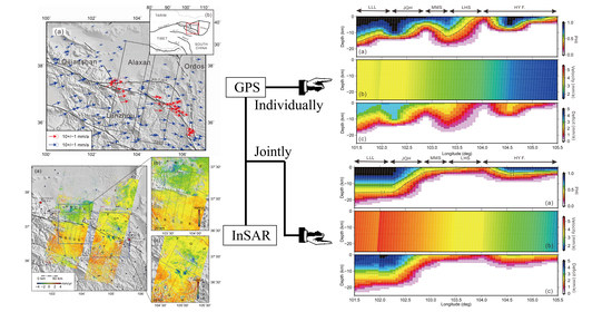
Elastic strain accumulated in the brittle seismogenic layer of the upper crust is the basis of earthquake occurrence, although activity in the deep ductile layer of the lower crust and upper mantle is also closely related to earthquake gestation [30]. The elastic rebound theory holds that the ductile lower crust and upper mantle are in a long-term stable slipping state, while the brittle layer in the upper crust experiences elastic strain accumulation due to fault coupling. When coseismic rupture occurs, elastic strain is released, and the relative motion between the brittle upper layer and the deep ductile layer tends to be uniform [30]. On this basis, the back-slip theory considers that the interseismic surface deformation rate of the boundary fault is relative movement rate of blocks on both sides of the fault minus the slip rate deficits due to fault coupling [29,31]. TDefnode is an inversion procedure based on the back-slip theory; it can be used to study the rotational motion of elastic lithosphere blocks, the fault locking degree of block boundaries, slip rate deficits, and other related parameters [32,33]. Based on the elastic half-space model [34], the grid search method and simulated annealing method can be used to determine the Euler pole of the block rotation motion, the fault locking degree, and the slip rate deficit of the block boundary. The fault locking degree is expressed by a pure dynamic scalar (hereafter referred to as PHI). When PHI is 1, the fault plane is completely locked; when it is 0, the fault plane is completely creeping; values between 0 and 1 mean that the fault plane is partially coupled. The slip rate deficit on the fault plane is the product of the long-term slip rate and the fault locking degree.
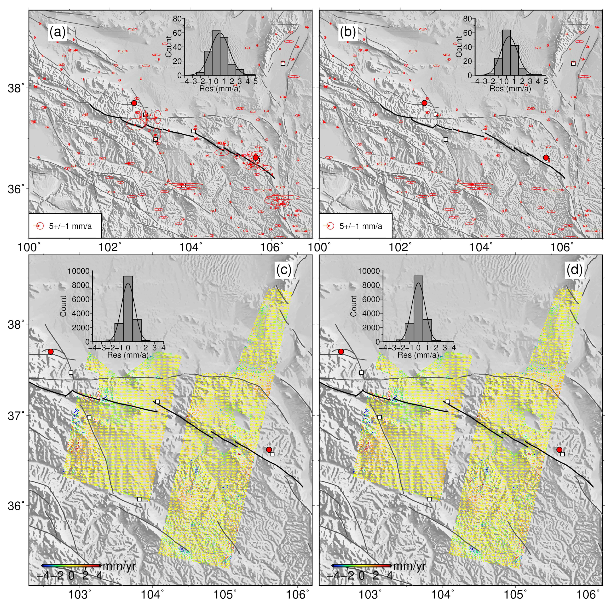
Based on previous GPS and geological studies of the active blocks [16,35], the area surrounding the Haiyuan fault zone is divided into four blocks: Ordos, Alaxan, Qilian, and Lanzhou (Figure 5b). The nodes of the fault plane refer to the surface traces of the Haiyuan fault zone drawn by [36] and correspond to the boundary of the blocks. The fault dip was set to 65° (dips to south) [16,37] and the fault depth range was set to 0–25 km. We controlled the 3D geometry of the fault by setting the nodes on the fault plane. The positions of the nodes were determined by the latitude, longitude, and depth. After the fault plane was determined, we divided it into a grid area of 5 km × 1 km and set the PHI value to monotonically decrease with depth [32]. We calculated the PHI value at each node using the TDefnode program and performed bilinear interpolation to obtain the PHI value of each grid region. The data fitting degree can be expressed by:
where n is the number of observations, m is the number of unknown parameters, r is the residual, and is the observation data error. The fault slip rate can be calculated from the relative angular velocity of motion of adjacent blocks. After acquiring the locking degree and slip rate on the fault plane, the slip rate deficit for each grid region can be found from the product of the two.
3.2. Inversion Constrainted by GPS and InSAR Alone and Jointly
3.2.1. Individual Inversion from GPS Data Only
Based on the back-slip block model, most previous inversions of the fault kinematic parameters have been constrainted by GPS alone [32,33]. However, the spatial distribution of GPS data in this region is sparse, and the resulting spatial resolution of the fault parameters is low. To obtain high-resolution kinematic parameters of the Haiyuan fault zone and verify the spatial constraint ability of GPS data to invert the fault kinematic parameters, we inverted the Haiyuan fault zone based on GPS and InSAR data.
We first used the GPS horizontal velocity field to invert the kinematic parameters of the Haiyuan fault zone. The distribution of the GPS data is shown in Figure 5. Most of the GPS data are 1999–2016 Crustal Movement Observation Network Of China (CMONOC) station observation data (blue arrows in Figure 5); the observation frequency is biennial. The dense GPS data near the Haiyuan fault zone (red arrows in Figure 5) are from near-field encryption stations deployed by our research group. We carried out annual campaign observations from 2013–2016, and obtained observation data for four consecutive years. In total, this study used data from 178 CMONOC GPS stations and 34 encrypted GPS stations. These GPS data were processed using GAMIT 10.40 software [38]. Together with data from 21 international GPS service (IGS) stations, raw pseudo-range and phase observations were first used to estimate satellite orbits parameters and daily loosely constrained station coordinates [37]. Then the daily solutions and the loosely constrained global solutions produced by the Scripps Orbital and Position Analysis Center (SOPAC) were combined to estimate seven parameters transformation under the ITRF2008 framework by using 34 globally distributed IGS stations. Therefore, the daily time series of each station in the ITRF2008 could be obtained. The positions and velocities were estimated based on the time series. Finally, the velocities were transformed into a Eurasia frame according to the Euler vector for Eurasia with respect to the ITRF2008 [39]. The velocities used in this study were listed in the Supplementary Materials.
The locking degree, slip rate, and slip rate deficit of the Haiyuan fault zone obtained based on GPS data inversion are shown in Figure 6. The inversion results show that the slip rate decreases gradually from west to east along the entire Haiyuan fault zone; the locking degree and locking depth show undulating local fluctuations, but generally exhibit a weakening trend from west to east. In the middle part of the LHS segment and to its west, the fault locking depth is 5–17 km; the eastern part of the LHS segment and the western and eastern parts of the 1920 Haiyuan rupture segments have shallower locking depths (1–5 km). That of the middle part of the 1920 Haiyuan rupture segments is in the range of 4 to 8 km. The long-term left-lateral strike-slip rate of the Haiyuan fault zone gradually decreases from west (4 mm/yr along the LLL segment) to east (1.9 mm/yr along the eastern part of the 1920 Haiyuan rupture segment). The slip rate deficit is mainly concentrated on the middle part of the LHS segment and its west sections; there is also some deficit on the middle part of the 1920 earthquake rupture zone.
3.2.2. Joint Inversion of GPS and InSAR Data
The amount of InSAR observation data is very large; the number of points is in the order of 100,000. Large volumes of redundant data seriously affect calculation efficiency. At the same time, there were also some non-tectonic deformation zones and noise points with lower coherence in the InSAR rate field. Therefore, it was necessary to pre-process and downsample the InSAR data before inversion. We first masked the obvious non-tectonic deformation area (funnel settlement area) and uncoherent area with the unwrapping error, and then divided the deformation field into 1’ × 1’ (longitude × latitude) grid cells. The average of the rate of each grid cell was obtained as the deformation rate of the cell, and the average value of the latitude and longitude of the region was calculated to represent the cell position. After downsampling, we obtained 9190 data points for track 290 and 6426 points for track 333.
We then used the pre-processed InSAR rate field data and the GPS data for a joint inversion (Figure 7). The variation in the locking degree along the entire Haiyuan fault zone is generally smooth, and fault locking mainly occurs in the west and east, and the west section is deeper than the east section. In the west, the locking depth gradually decreases from ∼17 km along the western LLL to the near surface along the middle part of the LHS. The eastern locking area mainly appears along the middle and eastern parts of the 1920 rupture segment, but the locking depth is only about 3–7 km. The western end of the 1920 rupture segment and the eastern end of the LHS are almost unlocked. The long-term left-lateral strike-slip rate of the Haiyuan fault zone gradually decreases from west (4.7 mm/yr on the LLL) to east (2.0 mm/yr on the eastern end of the 1920 rupture segment). The slip rate deficit is mainly concentrated on the sections to the west of MMS; however, there is also some slip rate deficit along the middle and eastern sections of the 1920 earthquake rupture segment (Figure 7a). The slip rate deficit of the LHS is very weak, especially in its east end where there is basically no slip rate deficit.
3.3. Comparison of Inversion Results of Different Data Combinations
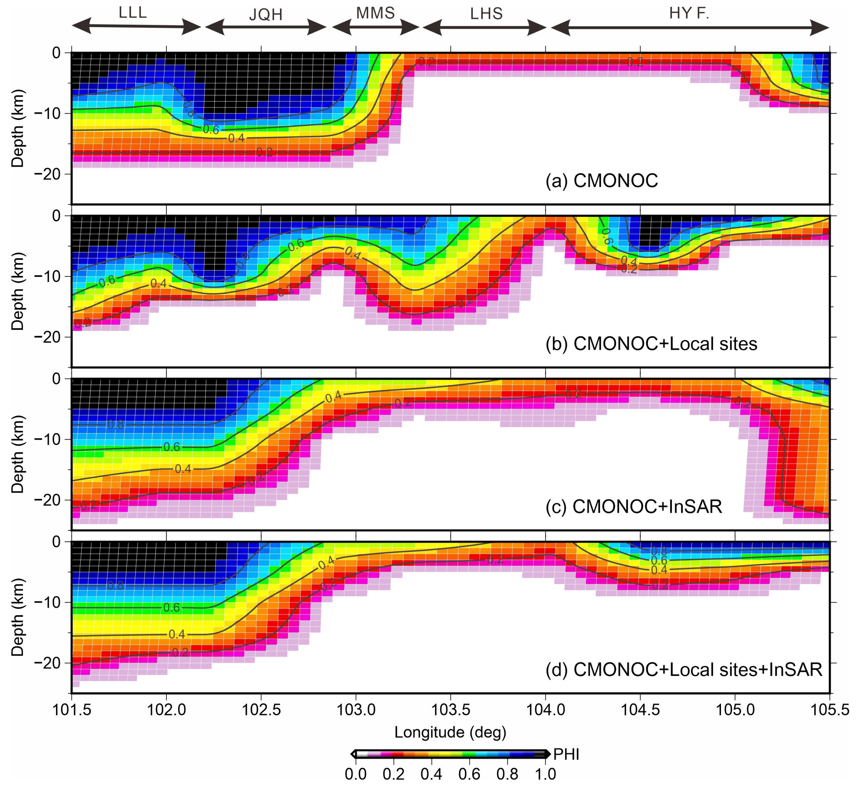
The GPS data used in the inversion consist of two parts. Data from the CMONOC are from sites more than 30 km apart and were collected over an 18-year period (1999–2016). In contrast, the encryption sites are densely distributed near the fault; the site spacing is mostly within 10 km and the observation time is only 4 years. To analyse the influence of different spatial densities of GPS data on the inversion results, we removed the encrypted site data and used only the sparse regional GPS data (Figure 5a). By comparing the results from the two inversions, we found significant differences in the locking degree (Figure 8a,b); after the encrypted observation data was removed, fluctuations along the fault were no longer evident.
The locking degree inverted from InSAR rate field data and GPS data after removing the encrypted stations are shown Figure 8c. The results are generally consistent with the combined inversion results using all of the GPS and InSAR data (Figure 8d). The entire fault zone can be separated into three regions with different locking degrees, but with a smooth transition across western, central, and eastern regions; the extent and depth of the strong western locking zone are basically the same as Figure 8a. Only the extent of the shallow weakly closed zone extends eastward, while the extent of the eastern locked zone decreases correspondingly and the locking depth increases to a depth of approximately 20 km.
The results of the two joint inversions (Figure 8c,d) are in good agreement, indicating that the dense, near continuous distribution of InSAR data plays a significant role and to some extent masks the influence of different GPS data densities. The InSAR data had a spatial resolution of 1.5 km even after downsampling, while the near-field encrypted GPS data point spacing was only ∼10 km. Therefore, the InSAR data strongly constrain the inversion results. At the same time, the consistency of the two joint inversion results shows that the selected fault model and inversion algorithm are stable and reliable. The central and eastern parts of Haiyuan Fault, which show some differences between the two inversions, are within the area of densely distributed GPS encryption stations; the results along this stretch of the fault confirm the constraining effect of near-field encrypted GPS stations.
The fault locking degree distribution characteristics obtained by different data combinations are similar in general, but also contain significant differences (Figure 8). The inversions of the four different datasets all show strong locking along the western MMS, with the locking depth mostly distributed from 5 to 17 km; along the eastern MMS to the 1920 rupture zone, the locking depth is very shallow (within a few kilometres of the surface). However, the addition of near-field encrypted GPS data causes local fluctuations of locking depth along the fault, and local deepening of the locking depth in the MMS–LHS segments and in the middle and eastern parts of the 1920 rupture segment (Figure 8b). Secondly, the joint inversion results using the high spatial resolution dense InSAR data (Figure 8c,d) show that the locking depth of the entire Haiyuan fault zone is relatively smooth; the local fluctuations caused by near-field encrypted GPS stations are no longer so obvious. Overall, the results are more consistent with those using just the sparse GPS data (Figure 8a). Our analysis indicates that the inversion results are closely related to the distribution and uniformity of the data points. The near-field encrypted GPS data are not evenly distributed along the fault zone, but are mainly concentrated along the MMS–LHS segments and along the middle and eastern parts of the 1920 rupture segment (Figure 5); this may be the cause of the wave-like fluctuations in the inversion results and the increased locking depths in these areas. The spatial resolution of InSAR data is high, data points are evenly distributed, and the data coverage is relatively large; this provides good constraints on the motion of the entire fault zone and that of different segments, making the inversion results more reliable.
The residuals and their 1- error (70% confidence level) between the GPS or InSAR data and the synthetic values obtained from two joint inversions are shown in Figure 9. The fitting results of GPS data are generally better (Figure 9a,b). The encrypted site fitting residuals and their 1- error are relatively large, which is due to the shorter observation period of encrypted sites (four years) compared to CMONOC sites. From the histogram, the GPS data fitting residuals for the two joint inversion results are concentrated around ±1.5 mm/yr, which indicates that the GPS simulation values can reflect the distribution characteristics of the GPS horizontal velocity field as a whole. The fitting residuals of InSAR data for the two joint inversions were basically the same and were concentrated around ±1.5 mm/yr. The data fitting results were good.
4. Discussion
4.1. Comparison with Existing InSAR Results
Our InSAR rate map of Haiyuan fault zone is in good agreement with the previous results [22]. We compared the deformation pattern in fault near field and profiles at the same locations and found that they are highly similar in shape and values (Figure 10 and Figure 11), indicating the reliability of our observations and further supporting the existence of creep in the Tianzhu seismic gap. Compared with the observations of [22], the long strip Envisat data used in this study cover a larger range in the north–south direction; furthermore, we used the StaMPS method to ensure a relatively stable PS point in the partially poor coherent region. Therefore, the deformation information revealed is more abundant.
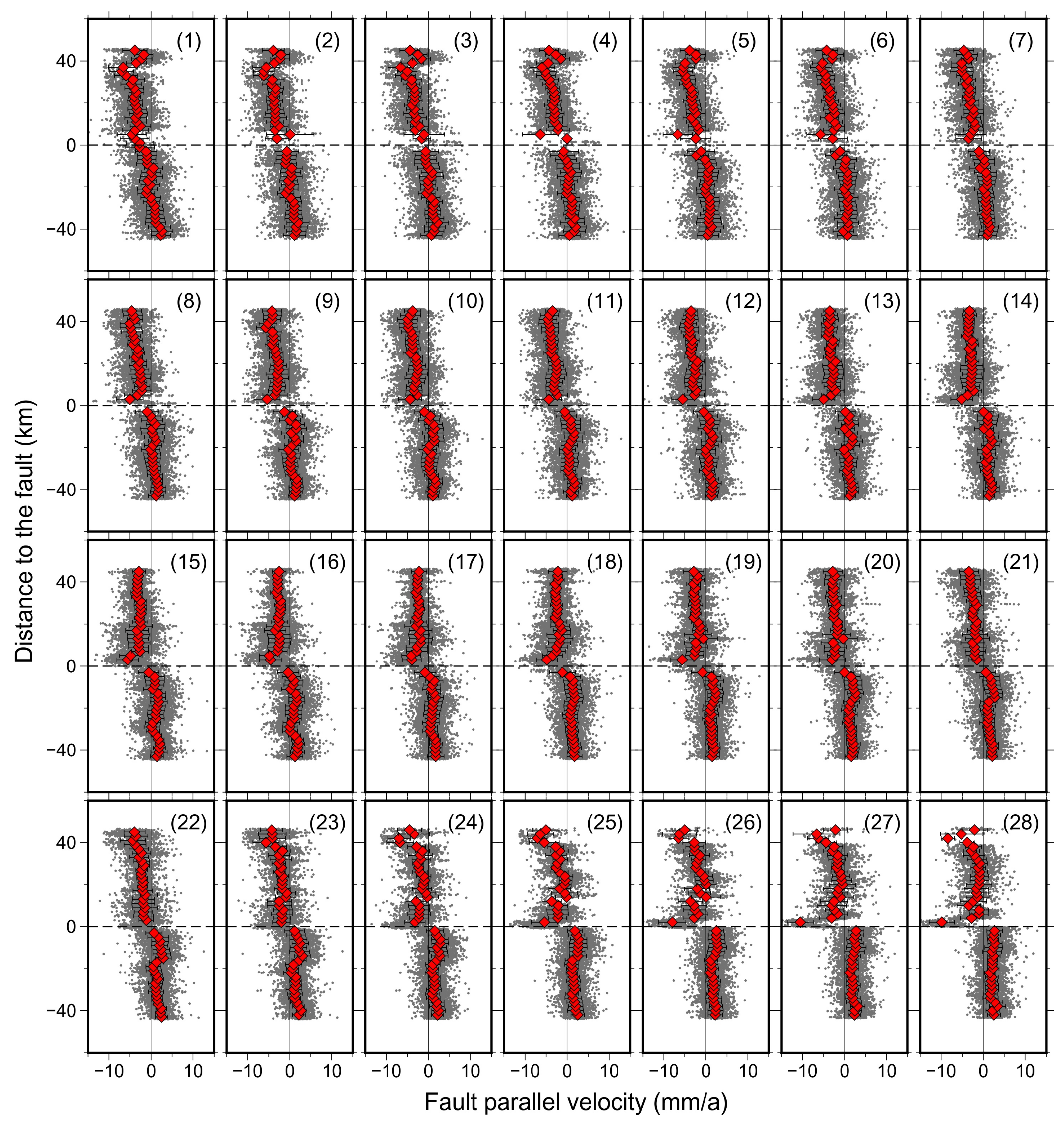
To accurately determine the length of the creep section, we built 28 velocity profiles perpendicular to the fault in the LHS segment based on observations of track 333. Each profile is 27 km in length including the middle and eastern segments of the LHS, covering CC’–EE’ in Figure 3. Profiles were spaced 1 km apart and their width was 2 km. We converted the LOS deformation rate into a horizontal strike-slip rate along the fault and calculated the average and 1- values (Figure 12). From Figure 12, velocity profiles at different locations are generally the same, but the deformation gradients across the fault from west to east show obvious changes. Profiles (1)–(6) show smooth cross-fault deformation, which is consistent with the near-field deformation characteristics of the interseismic coupling. Profiles (7)–(25) show a steep change in the rate of deformation across the fault over a distance of 19 km; this is consistent with near-field deformation of the interseismic creep. Profiles (26)–(28) show that the rate value on the north side is significantly larger in the near field than in the far field, suggesting that these profiles are related to the subsidence of the Jingtai Basin. Therefore, we suggest that the creeping part of the LHS is contained within a ∼19-km section west of the Jingtai Basin; this is less than the 35-km creep length obtained by [22]. Using the StaMPS method can retain a more complete short-wavelength signal, so the length of the creep segment obtained should be longer. However, the length of the creeping section we obtained is shorter than that of [22]. One possible reason is that the method of defining the creeping section is different. We use the cross-fault profile of the surface deformation to define the creep section, while [22] obtains the creep range by inverting the slip of the fault plane. However, due to the limitation of the Envisat data’s own longer spatio-temporal baseline, the acquired deformation field may have more uncoherence areas and other errors. The use of recent Sentinel-1 data can more accurately define the creeping extent.
4.2. Comparison with Previous Geological and GPS Results
To verify the accuracy and reliability of the obtained deformation rate field, the GPS horizontal deformation rate field of the area surrounding the Haiyuan fault zone was introduced for comparison. The GPS velocity field data were derived from [37]. Firstly, according to the geometric relationship between the GPS horizontal rate and the InSAR LOS deformation rate, GPS data were converted to the LOS direction, and the error was obtained according to the error propagation law. Secondly, the average LOS rate of InSAR data points within 2 km of GPS sites was calculated; the average value was taken as the InSAR observation value of the point and the 1- value was obtained (Figure 13). The difference between the InSAR observation results and the converted GPS results is basically distributed within the range of ±1 mm/yr. For the current range of InSAR measurement accuracy (∼1 mm/yr), the two agree well, indicating that the InSAR deformation rate field is reliable.
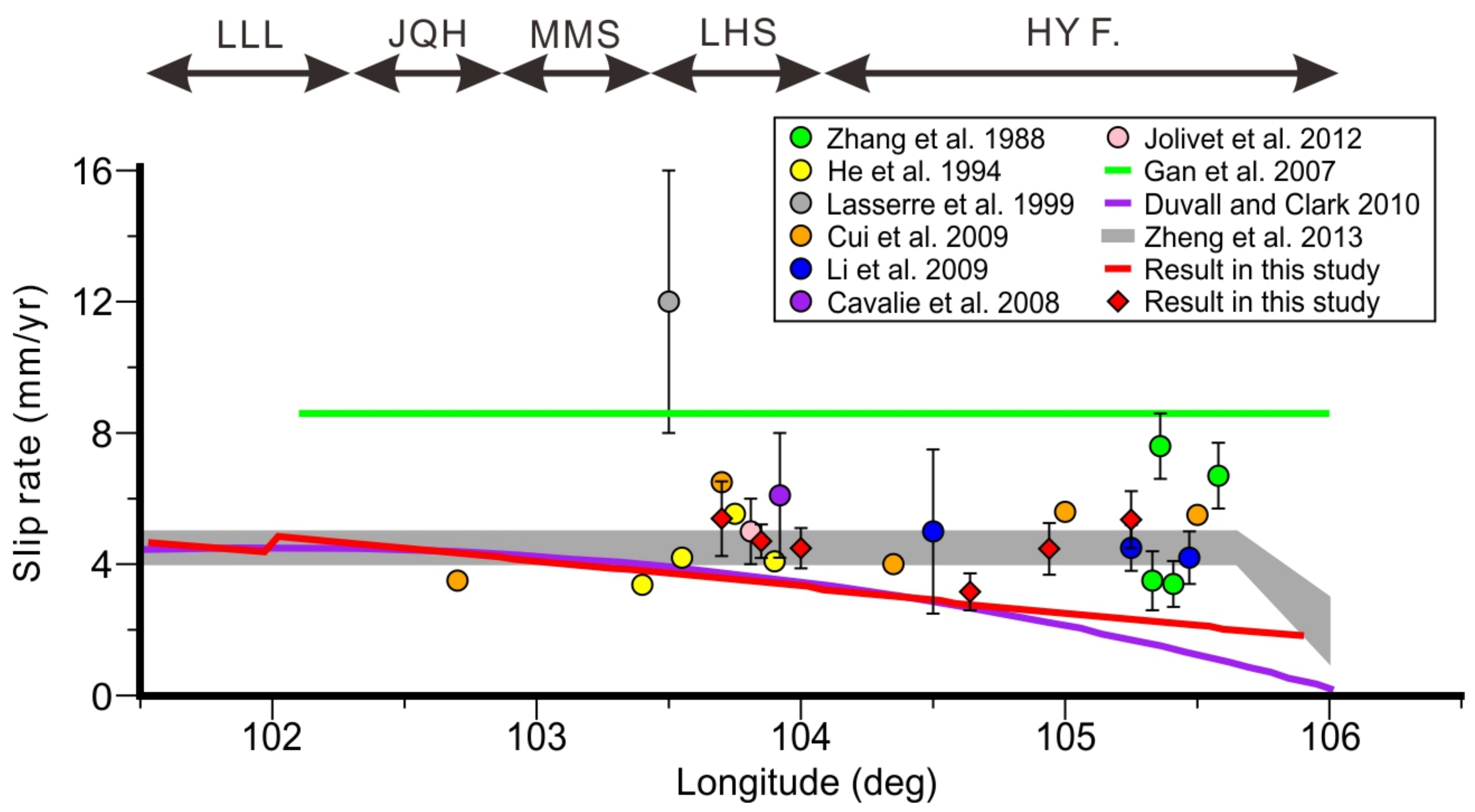
We also compared our results with earlier studies of geology and geodesy (Figure 14; [3,4,5,7,8,10,11,21,22,40]). The long-term slip rate obtained by our three-dimensional model based on block dislocations gradually decreases from west (4.7 mm/yr along the LLL) to east (2.0 mm/yr along the eastern part of the 1920 rupture segment; solid red line in Figure 14). This result is highly consistent with those of [10] using GPS data based on the elastic dislocation model (solid purple line in Figure 14). Along the western part of the 1920 rupture, the slip rates of both are almost completely coincident; for the middle and eastern parts of the 1920 rupture, our slip rate is slightly larger, but are closer to the results of most other studies. Based on the screw dislocation model, the deep slip rate (red diamonds in Figure 14) from LHS to the 1920 rupture segment fluctuates within the range of 3.2 to 7.6 mm/yr, which is consistent with the results of previous studies. At the same time, previous studies on the slip rate of the Haiyuan fault mainly focused on the LHS and on the eastern end of the fault zone; few studies have considered the fault to the west of LHS. In this study, the variation characteristics of the activity rate distribution for the entire Haiyuan fault zone were obtained; this compensates for the scarcity of observation points in the west.
Reference [11] used the Smith 3D model with GPS stations observation data from 1999 to 2007 near the Haiyuan fault zone as constraints, and obtained a locking depth of 22 km on the MMS and 10.3 km on the LHS. Ref. [16] used 1999–2013 GPS data based on the block model and obtained a locking depth of 9–23 km. When we used GPS and InSAR data for a joint inversion based on the back-slip block model, the locking depth obtained from the MMS to the middle of the LHS was significantly lower than that of previous estimates (1–4 km). However, when we used the same model but with only GPS as the data source, the obtained locking depth was 5–12 km, which is close to the results of previous studies. Therefore, we suggest that when GPS is used as the only data source, especially the GPS sites are sparse in the near-fault region, the constraint capability for local variations of fault slip rate and locking depth are limited. High spatial resolution InSAR data can supplement the lack of GPS sparse density, and this is beneficial for obtaining more reliable fault locking distributions. For the 1920 earthquake rupture segment, we obtained a locking depth of 3–7 km, which is consistent with the 3–6 km locking depth range obtained by [41]. The focal depth of 1920 Haiyuan earthquake is generally considered to be 17–20 km, suggesting that fault locking is likely to be in the depth range of 17 to 20 km. Our results are much shallower than this, which indicates that the middle–lower parts of the seismogenic upcrust layer of the 1920 rupture zone may not have fully recoupled. If this section is still in the postseismic stress adjustment stage, it explains why there has been no earthquake of magnitude 6.0 or above since 1920.
4.3. Constraint Effects of Different InSAR and GPS Datasets on Interseismic Inversion
By comparing the inversion results obtained under different datasets constrainted, it can be seen that the addition of InSAR data has a significant influence on the inversion results of local fault kinematic parameters. The GPS data cover a wide range with low and non-uniform distribution density, which can give good constraints on the relative motion of the overall block model. However, the movement of Haiyuan fault zone may be variant and complicated along the strike because of the disturbance of Haiyuan earthquake. The addition of InSAR data can address the shortcomings of GPS near-field data scarcity and allows for more reliable fault kinematic parameters. At the same time, a comparison of CMONOC GPS data and all GPS data inversions shows that the addition of encrypted GPS data significantly changes the inversion results, and gives the inversion results a wavy shape. We infer that the constraint effect of GPS data is not only related to the density of the stations, but also to the even distribution of those stations.
5. Conclusions
In this study, we used Envisat radar data from 2003 to 2010 to obtain the InSAR line-of-sight deformation rate field of the Haiyuan fault zone. The fault motion is characterised by left-lateral strike-slip. Analysis of high-density cross-fault deformation rate profiles on the Laohushan segment indicates a creep length of 19 km. Using the InSAR deformation rate from the Maomaoshan segment to the middle part of the 1920 rupture segment, combined with GPS observations, we obtained the fine slip rate and locking degree distribution characteristics of Haiyuan fault zone based on the screw dislocation model and the three-dimensional back-slip model, respectively. The results show that the shallow surface of the eastern LHS segment is in a creep state, while other segments are locked. The locking degree changes significantly along the strike with the western part reaching 17 km and the eastern part of 3–7 km. The long-term slip rate gradually decreases from west 4.7 mm/yr to east 2.0 mm/yr. The results of this study refine our understanding of the slip rates and locking degrees of different segments of the Haiyuan fault zone and provide reference information for regional seismic hazard assessment.
Supplementary Materials
The following are available online at https://0-www-mdpi-com.brum.beds.ac.uk/article/10.3390/rs13163333/s1, Dataset S1: CMONOC GPS velocities, Dataset S2: Encrypted GPS velocities.
Author Contributions
Conceptualization, C.Q. and X.S.; Formal analysis, X.Q. and D.Z.; Methodology, X.Q.; Software, X.Q.; Supervision, C.Q. and X.S.; Validation, X.Q., C.Q., D.Z., and L.L.; Visualization, X.Q.; Writing—original draft, X.Q.; Writing—review and editing, X.Q., C.Q., D.Z., and L.L. All authors have read and agreed to the published version of the manuscript.
Funding
This work was supported jointly by the National Key Laboratory of Earthquake Dynamics (LED2019A02), the Basic Scientific Funding of Institute of Geology, CEA (IGCEA1809, IGCEA2104) and the National Natural Science Foundation of China (41872229).
Institutional Review Board Statement
Not applicable.
Informed Consent Statement
Not applicable.
Data Availability Statement
Envisat/ASAR images can be downloaded from European Space Agency (ESA, http://esar-ds.eo.esa.int/sxcat, accessed on 21 August 2021). The GPS data used in this study can be obtained from supplementary materials.
Acknowledgments
We would like to thank the European Space Agency (ESA) for providing Envisat Advanced Synthetic Aperture Radar (ASAR) long strip data. Some figures were prepared using the public domain Generic Mapping Tools (GMT).
Conflicts of Interest
The authors declare that they have no known competing financial interest or personal relationships that could have appeared to influence the work reported in this paper.
References
- Gaudemer, Y.; Tapponnier, P.; Meyer, B.; Peltzer, G.; Shunmin, G.; Zhitai, C.; Huagung, D.; Cifuentes, I. Partitioning of crustal slip between linked, active faults in the eastern Qilian Shan, and evidence for a major seismic gap, the ‘Tianzhu gap’, on the western Haiyuan Fault, Gansu (China). Geophys. J. Int. 1995, 120, 599–645. [Google Scholar] [CrossRef] [Green Version]
- Jing, L.-Z.; Klinger, Y.; Xu, X.; Lasserre, C.; Chen, G.; Chen, W.; Tapponnier, P.; Zhang, B. Millennial recurrence of large earthquakes on the Haiyuan fault near Songshan, Gansu Province, China. Bull. Seismol. Soc. Am. 2007, 97, 14–34. [Google Scholar]
- Lasserre, C.; Morel, P.H.; Gaudemer, Y.; Tapponnier, P.; Ryerson, F.; King, G.; Métivier, F.; Kasser, M.; Kashgarian, M.; Liu, B.; et al. Postglacial left slip rate and past occurrence of M⩾8 earthquakes on the western Haiyuan fault, Gansu, China. J. Geophys. Res. Solid Earth 1999, 104, 17633–17651. [Google Scholar] [CrossRef] [Green Version]
- Li, C.; Zhang, P.; Yin, J.; Min, W. Late Quaternary left-lateral slip rate of the Haiyuan fault, northeastern margin of the Tibetan Plateau. Tectonics 2009, 28. [Google Scholar] [CrossRef]
- Zhang, P.; Molnar, P.; Burchfiel, B.C.; Royden, L.; Wang, Y.; Deng, Q.; Song, F.; Zhang, W.; Jiao, D. Bounds on the Holocene slip rate of the Haiyuan fault, north-central China. Quat. Res. 1988, 30, 151–164. [Google Scholar]
- Burchfiel, B.; Zhang, P.; Wang, Y.; Zhang, W.; Song, F.; Deng, Q.; Molnar, P.; Royden, L. Geology of the Haiyuan fault zone, Ningxia-Hui Autonomous Region, China, and its relation to the evolution of the northeastern margin of the Tibetan Plateau. Tectonics 1991, 10, 1091–1110. [Google Scholar] [CrossRef]
- Zheng, W.; Zhang, P.; He, W.; Yuan, D.; Shao, Y.; Zheng, D.; Ge, W.; Min, W. Transformation of displacement between strike-slip and crustal shortening in the northern margin of the Tibetan Plateau: Evidence from decadal GPS measurements and late Quaternary slip rates on faults. Tectonophysics 2013, 584, 267–280. [Google Scholar] [CrossRef]
- Gan, W.; Zhang, P.; Shen, Z.K.; Niu, Z.; Wang, M.; Wan, Y.; Zhou, D.; Cheng, J. Present-day crustal motion within the Tibetan Plateau inferred from GPS measurements. J. Geophys. Res. Solid Earth 2007, 112. [Google Scholar] [CrossRef] [Green Version]
- Thatcher, W. Microplate model for the present-day deformation of Tibet. J. Geophys. Res. Solid Earth 2007, 112. [Google Scholar] [CrossRef]
- Duvall, A.R.; Clark, M.K. Dissipation of fast strike-slip faulting within and beyond northeastern Tibet. Geology 2010, 38, 223–226. [Google Scholar] [CrossRef]
- Cui, D.; Wang, Q.; Hu, Y.; Wang, W.; Zhu, G. Inversion of GPS data for slip rates and locking depths of the Haiyuan fault. Acta Seismol. Sin. 2009, 31, 516–525. [Google Scholar]
- Le Béon, M.; Klinger, Y.; Al-Qaryouti, M.; Mériaux, A.S.; Finkel, R.C.; Elias, A.; Mayyas, O.; Ryerson, F.J.; Tapponnier, P. Early Holocene and Late Pleistocene slip rates of the southern Dead Sea Fault determined from 10Be cosmogenic dating of offset alluvial deposits. J. Geophys. Res. Solid Earth 2010, 115. [Google Scholar] [CrossRef]
- Papanikolaou, I.D.; Roberts, G.P.; Michetti, A.M. Fault scarps and deformation rates in Lazio–Abruzzo, Central Italy: Comparison between geological fault slip-rate and GPS data. Tectonophysics 2005, 408, 147–176. [Google Scholar] [CrossRef]
- Cowgill, E.; Gold, R.D.; Chen, X.; Wang, X.-F.; Arrowsmith, J.R.; Southon, J. Low Quaternary slip rate reconciles geodetic and geologic rates along the Altyn Tagh fault, northwestern Tibet. Geology 2009, 37, 647–650. [Google Scholar] [CrossRef]
- Qiao, X.; Zhou, Y. Geodetic imaging of shallow creep along the Xianshuihe fault and its frictional properties. Earth Planet. Sci. Lett. 2021, 567, 117001. [Google Scholar] [CrossRef]
- Li, Y.; Shan, X.; Qu, C.; Wang, Z. Fault locking and slip rate deficit of the Haiyuan-Liupanshan fault zone in the northeastern margin of the Tibetan Plateau. J. Geodyn. 2016, 102, 47–57. [Google Scholar] [CrossRef]
- Hao, M.; Li, Y.; Qin, S. Spatial and temporal distribution of slip rate deficit across Haiyuan-Liupan Shan fault zone constrained by GPS data. Seismol. Geol. 2017, 39, 471–484. [Google Scholar]
- Berardino, P.; Fornaro, G.; Lanari, R.; Sansosti, E. A new algorithm for surface deformation monitoring based on small baseline differential SAR interferograms. IEEE Trans. Geosci. Remote Sens. 2002, 40, 2375–2383. [Google Scholar] [CrossRef] [Green Version]
- Ferretti, A.; Prati, C.; Rocca, F. Nonlinear subsidence rate estimation using permanent scatterers in differential SAR interferometry. IEEE Trans. Geosci. Remote Sens. 2000, 38, 2202–2212. [Google Scholar] [CrossRef] [Green Version]
- Hooper, A. A multi-temporal InSAR method incorporating both persistent scatterer and small baseline approaches. Geophys. Res. Lett. 2008, 35. [Google Scholar] [CrossRef] [Green Version]
- Cavalié, O.; Lasserre, C.; Doin, M.P.; Peltzer, G.; Sun, J.; Xu, X.; Shen, Z.K. Measurement of interseismic strain across the Haiyuan fault (Gansu, China), by InSAR. Earth Planet. Sci. Lett. 2008, 275, 246–257. [Google Scholar] [CrossRef]
- Jolivet, R.; Lasserre, C.; Doin, M.P.; Guillaso, S.; Peltzer, G.; Dailu, R.; Sun, J.; Shen, Z.K.; Xu, X. Shallow creep on the Haiyuan fault (Gansu, China) revealed by SAR interferometry. J. Geophys. Res. Solid Earth 2012, 117. [Google Scholar] [CrossRef] [Green Version]
- Jolivet, R.; Lasserre, C.; Doin, M.P.; Peltzer, G.; Avouac, J.P.; Sun, J.; Dailu, R. Spatio-temporal evolution of aseismic slip along the Haiyuan fault, China: Implications for fault frictional properties. Earth Planet. Sci. Lett. 2013, 377, 23–33. [Google Scholar] [CrossRef]
- Daout, S.; Jolivet, R.; Lasserre, C.; Doin, M.P.; Barbot, S.; Tapponnier, P.; Peltzer, G.; Socquet, A.; Sun, J. Along-strike variations of the partitioning of convergence across the Haiyuan fault system detected by InSAR. Geophys. Suppl. Mon. Not. R. Astron. Soc. 2016, 205, 536–547. [Google Scholar] [CrossRef]
- Ferretti, A.; Prati, C.; Rocca, F. Multibaseline InSAR DEM reconstruction: The wavelet approach. IEEE Trans. Geosci. Remote Sens. 1999, 37, 705–715. [Google Scholar] [CrossRef]
- Hooper, A.; Zebker, H.; Segall, P.; Kampes, B. A new method for measuring deformation on volcanoes and other natural terrains using InSAR persistent scatterers. Geophys. Res. Lett. 2004, 31. [Google Scholar] [CrossRef]
- Hooper, A.J. Persistent Scatter Radar Interferometry for Crustal Deformation Studies and Modeling of Volcanic Deformation; Stanford University: Stanford, CA, USA, 2006. [Google Scholar]
- Zhang, P.Z.; Shen, Z.; Wang, M.; Gan, W.; Bürgmann, R.; Molnar, P.; Wang, Q.; Niu, Z.; Sun, J.; Wu, J.; et al. Continuous deformation of the Tibetan Plateau from global positioning system data. Geology 2004, 32, 809–812. [Google Scholar] [CrossRef]
- Savage, J.C. A dislocation model of strain accumulation and release at a subduction zone. J. Geophys. Res. Solid Earth 1983, 88, 4984–4996. [Google Scholar] [CrossRef]
- Scholz, C.H. Earthquakes and friction laws. Nature 1998, 391, 37–42. [Google Scholar] [CrossRef]
- Matsu’ura, M.; Jackson, D.D.; Cheng, A. Dislocation model for aseismic crustal deformation at Hollister, California. J. Geophys. Res. Solid Earth 1986, 91, 12661–12674. [Google Scholar] [CrossRef]
- McCaffrey, R.; Stein, S.; Freymueller, J. Crustal block rotations and plate coupling. Plate Bound. Zones Geodyn. Ser 2002, 30, 101–122. [Google Scholar]
- McCaffrey, R.; Qamar, A.I.; King, R.W.; Wells, R.; Khazaradze, G.; Williams, C.A.; Stevens, C.W.; Vollick, J.J.; Zwick, P.C. Fault locking, block rotation and crustal deformation in the Pacific Northwest. Geophys. J. Int. 2007, 169, 1315–1340. [Google Scholar] [CrossRef] [Green Version]
- Okada, Y. Surface deformation due to shear and tensile faults in a half-space. Bull. Seismol. Soc. Am. 1985, 75, 1135–1154. [Google Scholar] [CrossRef]
- Wang, W.; Qiao, X.; Yang, S.; Wang, D. Present-day velocity field and block kinematics of Tibetan Plateau from GPS measurements. Geophys. J. Int. 2017, 208, 1088–1102. [Google Scholar] [CrossRef]
- Deng, Q. Chinese Active Tectonic Map; Seismological Press: Beijing, China, 2007. [Google Scholar]
- Li, Y.; Shan, X.; Qu, C.; Zhang, Y.; Song, X.; Jiang, Y.; Zhang, G.; Nocquet, J.M.; Gong, W.; Gan, W.; et al. Elastic block and strain modeling of GPS data around the Haiyuan-Liupanshan fault, northeastern Tibetan Plateau. J. Asian Earth Sci. 2017, 150, 87–97. [Google Scholar] [CrossRef]
- Herring, T.; King, R.; McClusky, S. GAMIT Reference Manual, Release 10.4; Massachusetts Institute of Technology: Cambridge, UK, 2010. [Google Scholar]
- Altamimi, Z.; Collilieux, X.; Métivier, L. ITRF2008: An improved solution of the international terrestrial reference frame. J. Geod. 2011, 85, 457–473. [Google Scholar] [CrossRef] [Green Version]
- He, W.; Liu, B.; Lu, T.; Yuan, D.; Liu, J.; Liu, X. Study on the segmentation of Laohushan fault zone. Northwest. Seismol. J. 1994, 16, 66–72. [Google Scholar]
- Song, X.; Jiang, Y.; Shan, X.; Gong, W.; Qu, C. A fine velocity and strain rate field of present-day crustal motion of the Northeastern Tibetan Plateau inverted jointly by InSAR and GPS. Remote Sens. 2019, 11, 435. [Google Scholar] [CrossRef] [Green Version]
Figure 1.
Tectonic setting of the Haiyuan fault zone. Red dots denote the epicentres of the 1920 M8.5 Haiyuan earthquake and the 1927 M8.0 Gulang earthquake. The red solid line denotes the rupture section of the Haiyuan earthquake, and the red dotted ellipse is the possible rupture area of the Gulang earthquake. The blue line denotes the Tianzhu seismic gap. Brown dots denote earthquakes of M5 or above (1920–2016), and white dots denote earthquakes of <M5 (1970–2016). White squares denote the locations of cities. The black rectangle is the coverage of the InSAR data. LLL: Lenglongling segment; JQH: Jinqianghe segment; MMS: Maomaoshan segment; LHS: Laohushan segment.

Figure 2.
Temporal-spatial baseline networks of (a) T333 and (b) T290.

Figure 3.
(a) Average line-of-sight (LOS) velocity map from tracks 333 and 290. (b,c) are local zoom areas cross the fault. Red dots denote the epicentres of the 1920 M8.5 Haiyuan earthquake and the 1927 M8.0 Gulang earthquake. Grey solid lines denote other fault traces. Black dotted lines denote 2-km wide velocity profiles. Purple triangles represent global positioning system (GPS) stations. White squares denote the locations of cities. HYF.: the 1920 Haiyuan earthquake rupture segment; GL F.: Gulang fault; XS-TJS F.: Xiangshan-Tianjingshan fault; JQH: Jinqianghe segment; MMS: Maomaoshan segment; LHS: Laohushan segment.

Figure 4.
Fault-parallel velocity profiles and screw dislocation model fitting results. (AA’–HH’) Profiles shown in Figure 3. Grey points denote fault-parallel velocities along the fault transformed by InSAR LOS observations. Red diamonds are average values of the data within 2 km along the profile; error bars are the 1- errors. Blue lines are best fit curves, V represents the best fit slip rate in depth, D represents the optimal fit locking depth, and the dashed lines denote the position of the fault surface trace.

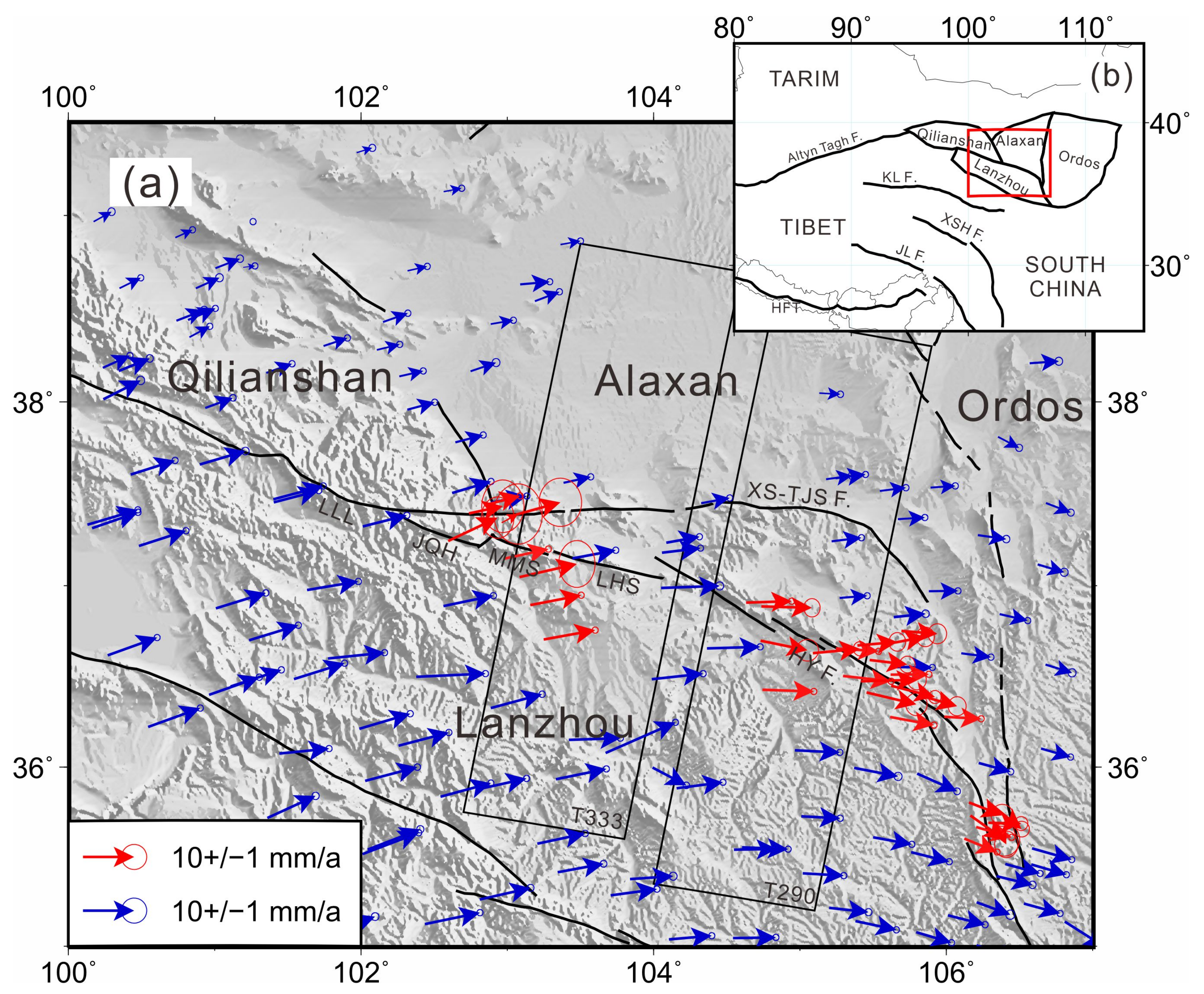
Figure 5.
Global positioning system (GPS) velocity field and block division of the Haiyuan fault zone. (a) GPS velocity field along the Haiyuan fault zone relative to the stable Eurasian plate, and (b) tectonic divisions of the surrounding area (Qilianshan block, Alaxan block, Lanzhou block, and Ordos block). The red box in (b) denotes the area shown in (a). Blue arrows are the results of observations from 1999–2016 recorded at GPS stations of the China Crustal Movement Observation Network (CMONOC); red arrows are the results of 2013–2016 campaign-mode observation from our group [37]. Black rectangles are the coverage of tracks 333 and 290. Error ellipses represent a 95% confidence level.

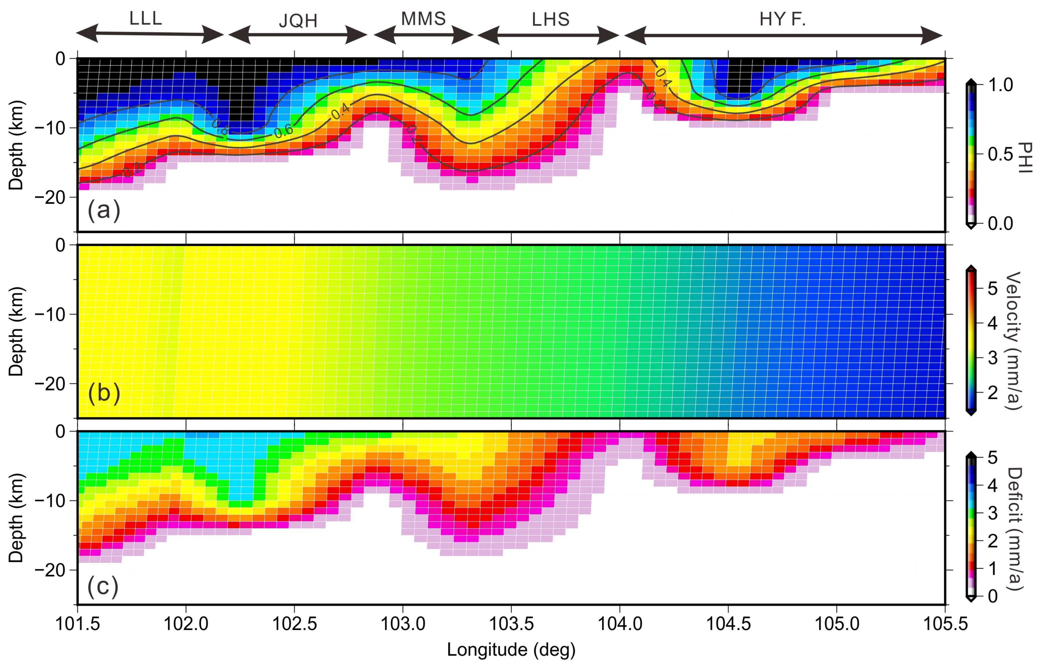
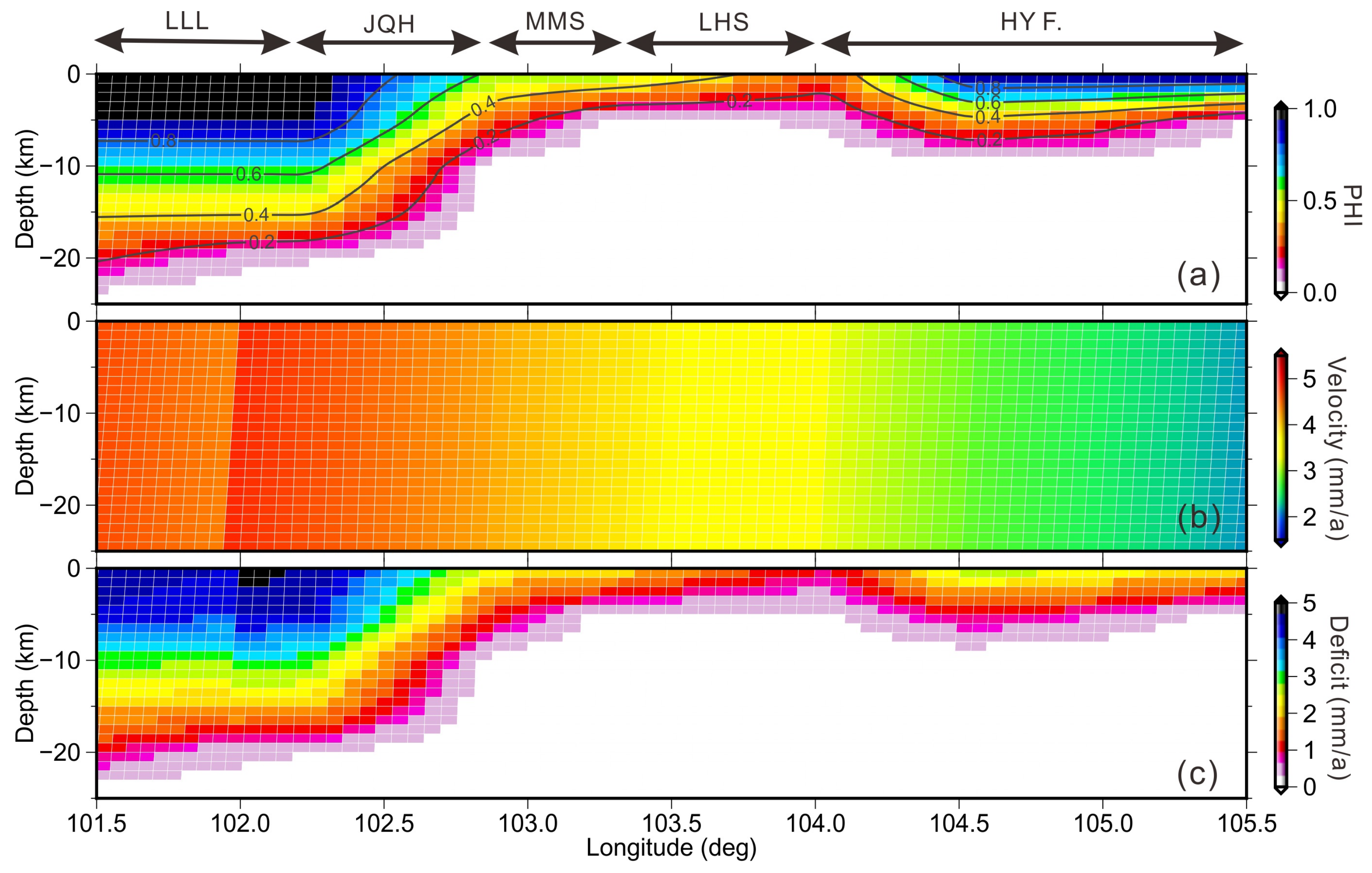
Figure 6.
Inversion results using all global positioning system (GPS) data. (a) Locking degree of the fault, (b) relative slip rate, and (c) slip rate deficit. LLL: Lenglongling segment; JQH: Jinqianghe segment; MMS: Maomaoshan segment; LHS: Laohushan segment; HY F.: the 1920 Haiyuan earthquake rupture segment; PHI: fault locking degree.

Figure 7.
Joint inversion results constrained by all GPS and InSAR. (a) Locking degree along the fault, (b) relative slip rate, and (c) slip rate deficit. LLL: Lenglongling segment; JQH: Jinqianghe segment; MMS: Maomaoshan segment; LHS: Laohushan segment; HY F.: the 1920 Haiyuan earthquake rupture segment; PHI: fault locking degree.

Figure 8.
Fault locking degree distributions inverted from different data combinations. (a) GPS data only from CMONOC, (b) GPS data from CMONOC and local dense sites built by our group, (c) CMONOC GPS data and InSAR data, and (d) all GPS and InSAR data. PHI: fault locking degree.
Figure 8.
Fault locking degree distributions inverted from different data combinations. (a) GPS data only from CMONOC, (b) GPS data from CMONOC and local dense sites built by our group, (c) CMONOC GPS data and InSAR data, and (d) all GPS and InSAR data. PHI: fault locking degree.

Figure 9.
Data fitting residuals of the GPS and InSAR joint inversions. (a,c) represent GPS and InSAR residuals of the joint inversion using all GPS and InSAR data, respectively. (b,d) represent GPS and InSAR residuals of the joint inversion using CMONOC sites and InSAR data, respectively. Black and grey solid lines denote fault traces. Red dots denote the epicentres of the 1920 M8.5 Haiyuan earthquake and the 1927 M8.0 Gulang earthquake. White squares denote the locations of cities.

Figure 10.
Comparison of deformation rate map across Haiyuan fault with previous research results. (a,c) Results from this study, and (b,d) deformation fields obtained by [22].
Figure 10.
Comparison of deformation rate map across Haiyuan fault with previous research results. (a,c) Results from this study, and (b,d) deformation fields obtained by [22].

Figure 11.
Comparison of InSAR LOS velocity results along cross fault profiles. (a,c) are results of [22]. (b,d) are results of this study. Profile locations are shown in Figure 10a. Red diamond denotes average values within 1 km along the profiles and error bar is their standard deviation.

Figure 12.
Fault-perpendicular velocity profiles evolution along the Laohushan (LHS) segment based on observations of track 333. The 28 profiles go from west to east; profiles (1) and (28) are the CC’ and EE’ profiles in Figure 3, respectively. Grey points are fault-parallel velocities along the fault transformed using interferometric synthetic aperture radar (InSAR) line-of-sight (LOS) velocities. Red diamonds denote the average values of the data within 2 km along the profile; error bars are the 1- error. Black dashed lines denote the fault location.

Figure 13.
Comparison of InSAR LOS observations and converted GPS values. (a) Track 333 and (b) track 290. Shaded areas denote error within ±1 mm/yr.
Figure 13.
Comparison of InSAR LOS observations and converted GPS values. (a) Track 333 and (b) track 290. Shaded areas denote error within ±1 mm/yr.

Figure 14.
Summary of the slip rate along the Haiyuan fault zone. The red solid line is the long-term slip rate of the Haiyuan fault zone obtained using the back-slip model; red diamonds are the slip rate of the fault obtained using the screw dislocation model. Other symbols and lines denote the results of previous studies (see figure legend for details). LLL: Lenglongling segment; JQH: Jinqianghe segment; MMS: Maomaoshan segment; LHS: Laohushan segment; HY F.: 1920 Haiyuan earthquake rupture segment.

Publisher’s Note: MDPI stays neutral with regard to jurisdictional claims in published maps and institutional affiliations. |
© 2021 by the authors. Licensee MDPI, Basel, Switzerland. This article is an open access article distributed under the terms and conditions of the Creative Commons Attribution (CC BY) license (https://creativecommons.org/licenses/by/4.0/).
Share and Cite
MDPI and ACS Style
Qiao, X.; Qu, C.; Shan, X.; Zhao, D.; Liu, L. Interseismic Slip and Coupling along the Haiyuan Fault Zone Constrained by InSAR and GPS Measurements. Remote Sens. 2021, 13, 3333. https://0-doi-org.brum.beds.ac.uk/10.3390/rs13163333
AMA Style
Qiao X, Qu C, Shan X, Zhao D, Liu L. Interseismic Slip and Coupling along the Haiyuan Fault Zone Constrained by InSAR and GPS Measurements. Remote Sensing. 2021; 13(16):3333. https://0-doi-org.brum.beds.ac.uk/10.3390/rs13163333
Chicago/Turabian StyleQiao, Xin, Chunyan Qu, Xinjian Shan, Dezheng Zhao, and Lian Liu. 2021. "Interseismic Slip and Coupling along the Haiyuan Fault Zone Constrained by InSAR and GPS Measurements" Remote Sensing 13, no. 16: 3333. https://0-doi-org.brum.beds.ac.uk/10.3390/rs13163333
Note that from the first issue of 2016, this journal uses article numbers instead of page numbers. See further details here.