
Hybrid Spatial–Temporal Graph Convolutional Networks for On-Street Parking Availability Prediction


1
School of Telecommunications Engineering, Xidian University, Xi’an 710071, China
2
The State Key Laboratory of Integrated Services Networks, Xidian University, Xi’an 710071, China
3
School of Computer Science and Technology, Xidian University, Xi’an 710071, China
4
School of Computing Technologies, RMIT University, Melbourne, VIC 3000, Australia
*
Author to whom correspondence should be addressed.
Remote Sens. 2021, 13(16), 3338; https://0-doi-org.brum.beds.ac.uk/10.3390/rs13163338
Submission received: 29 June 2021
/
Revised: 15 August 2021
/
Accepted: 18 August 2021
/
Published: 23 August 2021
(This article belongs to the Special Issue Data Mining and Machine Learning in Urban Applications)
Abstract
:With the development of sensors and of the Internet of Things (IoT), smart cities can provide people with a variety of information for a more convenient life. Effective on-street parking availability prediction can improve parking efficiency and, at times, alleviate city congestion. Conventional methods of parking availability prediction often do not consider the spatial–temporal features of parking duration distributions. To this end, we propose a parking space prediction scheme called the hybrid spatial–temporal graph convolution networks (HST-GCNs). We use graph convolutional networks and gated linear units (GLUs) with a 1D convolutional neural network to obtain the spatial features and the temporal features, respectively. Then, we construct a spatial–temporal convolutional block to obtain the instantaneous spatial–temporal correlations. Based on the similarity of the parking duration distributions, we propose an attention mechanism called to measure the similarity of parking duration distributions. Through the mechanism, we add the long-term spatial–temporal correlations to our spatial–temporal convolutional block, and thus, we can capture complex hybrid spatial–temporal correlations to achieve a higher accuracy of parking availability prediction. Based on real-world datasets, we compare the proposed scheme with the benchmark models. The experimental results show that the proposed scheme has the best performance in predicting the parking occupancy rate.
1. Introduction
With the rapid growth of the population and the economy in today’s cities, the number of vehicles in cities is rising and, with it, the demand for parking spaces. On-street parking is often a more cost-effective choice than parking facilities, such as garages and off-street parking bays. However, the number of on-street parking bays cannot keep up with the rising demand of the rapid growth of vehicles. Therefore, it is even harder to find available parking spaces, which makes parking an important issue that cannot be ignored today. On average, parking coverage takes 31% of land use in big cities [1]. Moreover, for some big cities, such as Los Angeles and Melbourne, the rates are up to 81% and 76%, respectively [2]. In many cities, smart parking is always an important issue to work on in both the research field and in economic developments. On-street parking is often a cost-effective choice compared to parking facilities, such as garages and off-street parking bays. However, with the rapid development of the urban economy, the problem of finding suitable parking bays has become more and more serious. First, the increasing number of motor vehicles has increased the demand for parking spaces. Second, some on-street parking information is not made public, and such information cannot be fully utilized, thus increasing the scarcity of parking spaces. Finally, the efficiency of on-street parking management is not high enough, which further reduces the utilization efficiency of urban parking spaces. There is a study showing that in big cities, on average, it takes nearly 20 min to find a free parking space [3]. The above issues have caused on-street parking to a be problem in recent years. To be specific, the difficulty in finding available parking spaces reduces the efficiency of urban operations and causes much pollution. It is also one of the most important causes of urban congestion [4]. It is reported that more than one-third of the traffic congestion in urban areas is caused by looking for free parking spaces [5].
On-street parking availability prediction results can provide drivers with useful and timely information and can help improve the utilization efficiency of urban parking spaces. So, it is of great significance to make stable and effective predictions. In general, parking availability prediction is one of the foundations of urban traffic control and guidance, which is also one of the main functions of an Intelligent Transportation System (ITS).
Historical data are required in order to predict parking availability. In the past, due to networks, equipment, and technical reasons, parking information was not completely recorded. In recent years, with the rapid development of Internet-of-Things (IoT) technologies, many cities have built or are building monitoring systems to record real-time on-street parking events. Such monitoring systems are networks of numerous in-ground sensors [6,7]. With such monitoring systems, plenty of historical data from on-street parking events are available to predict future parking availability.
Previous studies of prediction methods can be divided into two categories, which are knowledge-driven methods and data-driven methods. Knowledge-driven methods require suitable systematic programming and are suitable for some simple problems. However, parking prediction is a complex problem. Firstly, parking data change rapidly; thus, it is hard to model the parking prediction problem in big cities. Secondly, parking data are affected by many factors. For example, the parking occupancy rate (POR) on weekdays differs from that on weekends. Population distribution, schools, hospitals, etc. can also affect parking.
For data-driven methods, there are two common kinds of approaches, i.e., the conventional statistical approaches and machine learning approaches. The conventional statistical approaches, e.g., the autoregressive integrated moving average model (ARIMA) [8], have performed well in short-term prediction. However, due to the complexity of geographical locations, there is a high complexity and too much uncertainty in parking prediction. Therefore, for long-term prediction, conventional statistical approaches often fail to obtain a high prediction accuracy. Moreover, higher prediction accuracy and more complex modeling can be achieved by using machine learning methods, such as support vector regression (SVR) [9] and the k-nearest neighbors algorithm (KNN) [10]. However, most machine learning studies do not pay attention to the impact of contextual features of on-street parking bays, which play an important role in predicting the POR.
In recent years, deep learning methods have achieved great success in parking availability prediction. For example, long short-term memory (LSTM) [11,12], a variant of the recurrent neural network (RNN), is good at processing time-series data, such as POR data. However, parking availability prediction is not only a time-series problem, but it also shows a strong spatial correlation. Specifically, the parking conditions of parking areas are influenced by those of other parking areas. When many vehicles are parking in one parking area, other vehicles tend to park in another more available parking areas. It is hard for RNN-based methods to take advantage of spatial features. Instead, the combination of LSTM and convolutional neural networks (CNNs) [13] can be used to take advantage of temporal features and extract spatial features for predictions [14]. These methods can only be used for Euclidean data, such as images and voice signals; however, like traffic networks and social networks, on-street parking areas are distributed in a non-Euclidean space. Therefore, the above-mentioned methods still do not predict the POR of parking areas very well.
Recently, some prediction approaches based on the graph theory that can be used for non-Euclidean structures, such as traffic flow data, have been proposed [15,16,17]. However, these methods treat spatial correlations and temporal correlations separately. Therefore, the spatial–temporal correlations still need to be solved. In addition, these methods involve high computational complexity and, thus, require too much time for training. Spatio-temporal graph convolutional networks (STGCNs) [18] can jointly extract spatial and temporal features from the input and reduce the computational complexity with the first-order approximation of the Laplacian [19]. However, these traffic flow predictions only focus on instantaneous spatial–temporal correlations. For POR prediction tasks, they involve long-term spatial–temporal correlations, which means that spatial features are closely related to the periods of parking durations. For example, in rural areas, the parking durations may be longer, whereas in an urban area or the central business district (CBD) of a city, drivers often tend to spend less time in parking.
In this paper, we propose a hybrid spatial–temporal scheme that combines the instantaneous spatial–temporal correlations and the long-term spatial–temporal correlations. Specifically, we propose a novel deep learning architecture, the hybrid spatial–temporal graph convolutional networks (HST-GCNs). In this architecture, we first construct a temporal gated convolutional block (TGCB), which contains gated linear units (GLUs) and a 1D CNN, to capture the temporal features. Then, we construct a graph convolutional block by using graph convolution networks (GCNs) to capture the global spatial contextual features. In order to extract the instantaneous spatial–temporal correlations, we construct a spatial–temporal convolutional block, which contains two temporal gated convolutional blocks and one graph convolutional block in the middle, to control the inputs and outputs of the graph. Additionally, an attention mechanism called is added to the graph to model the spatial correlations. The attention mechanism can measure the similarity of parking duration distributions and add long-term spatial–temporal correlations to the HST-GCN architecture. To test the scheme, we collected real parking datasets from Melbourne in 2017. The datasets were affected by many factors, such as schools, hospitals, weather, and residential areas. Since it is difficult to consider single factors while keeping other factors constant, we considered these variables as an indivisible whole. Our experiments and our evaluation of the datasets show that the proposed HST-GCN framework outperforms state-of-the-art baselines when predicting the POR of areas with different time horizons. In summary, this paper makes the following contributions:
- We propose the hybrid spatial–temporal graph convolutional network (HST-GCN) framework for parking availability prediction. In the HST-GCNs, we adopt a 1D convolution and gated linear units (GLUs) to model instantaneous temporal features and use graph convolutional networks (GCNs) to capture the global spatial features. Then, we use the spatial–temporal convolutional block to capture the instantaneous spatial–temporal correlations.
- We propose a graph attention network and integrate into the spatial–temporal convolutional block, which also adds long-term spatial–temporal correlations into the HST-GCN architecture and helps obtain a stable prediction result.
- We conducted extensive experiments on a large-scale real-world dataset, and the experimental results demonstrated that the proposed framework outperformed state-of-the-art baselines when predicting the POR of areas with different time horizons.
The remainder of the paper is organized as follows. In Section 2, we introduce some baseline and graph-based prediction methods. In Section 3, we introduce the preliminaries of the study, including the definition of POR, graph construction, parking duration distributions, and problem definition. In Section 4, we introduce the designed scheme for predicting the POR. In Section 5, based on the real-world datasets, we carry out experiments to evaluate the performance of the proposed scheme. Finally, in Section 6, we present our conclusions and future work.
2. Related Work
2.1. Parking Availability Prediction
Parking availability prediction issues have been studied for years. The statistical models used for parking availability prediction include the historical average (HA), ARIMA [20], and linear regression (LR) [21]. These methods perform well in short-term predictions. However, there is too much uncertainty and complexity in parking events, thus making it unsuitable for these methods to perform long-term prediction tasks.
Machine learning methods can solve more complex problems. Therefore, they are also used for parking availability prediction. Bock et al. [22] used a two-step approach to predict parking space availability by using SVR methods, which showed a better performance than that of the one-step SVR model. Vlahogianni et al. [23] proposed a neural network (NN)-based model—called multi-layer perception (MLP)—to predict the occupancy rate of parking spaces. This model captured the temporal evolution of parking occupancy and accurately predicted occupancy up to half an hour ahead. Zheng et al. [24] performed a comparative analysis of the regression tree, NN, and SVR methods for the prediction of the POR and found that the regression tree method outperformed the other two algorithms that they evaluated. However, these machine learning methods did not jointly consider spatial–temporal patterns.
In recent years, deep learning methods have been widely used for parking availability prediction. Arjona et al. adopted the gated recurrent unit (GRU), a recurrent neural network method, for parking availability prediction according to a real scenario in the city of Riyadh. Shao et al. [12] proposed an LSTM model to predict parking multiple steps ahead and used the historical on-street POR in a specific region and the probability of car leaving to predict the parking availability in the future. However, the spatial correlations in the above studies were ignored.
2.2. Graph-Based Methods for Predictions
Graph-based methods can convert non-Euclidean data, which cannot be directly processed by classical CNN methods, into graph structure data, and then use the data for prediction. Therefore, graph-based methods have recently attracted much attention in the traffic prediction domain. Yang et al. [25] proposed a model that leveraged graph-convolutional neural networks (GCNNs) to extract the spatial relations of traffic flow in large-scale networks and utilized LSTM to capture the temporal features. Their model showed a better performance than that of the baselines, including the multi-layer LSTM and least absolute shrinkage and selection operator (LASSO). However, their model still could not extract the spatial and temporal correlations jointly. Li et al. [17] proposed a model named the diffusion convolutional recurrent neural network (DCRNN), which modeled the traffic flow as a diffusion process to predict the traffic flow. This model could incorporate both spatial and temporal dependency to enhance prediction performance. Zhao et al. [15] proposed a temporal graph convolutional network (T-GCN) for traffic prediction. They combined a GCN with a gated recurrent unit (GRU) to capture spatial and temporal correlations. Yu et al. [18] proposed a framework, the spatio-temporal graph convolutional networks (STGCNs), for forecasting traffic flow. The framework effectively captured comprehensive spatio-temporal correlations jointly by modeling multi-scale traffic networks and improved the training efficiency by using Chebyshev polynomial approximation and first-order approximation [19].
2.3. Attention Mechanisms on Graphs
Attention mechanisms have many benefits on graphs, including efficient computation and parallelization across all nodes in the graph. They also do not require knowledge of the entire graph structure up front [26]. Therefore, they have been widely used in recent prediction studies. Guo et al. [27] proposed the attention-based spatial–temporal graph convolutional network (ASTGCN) model, which adopted a spatial–temporal attention mechanism to capture dynamic spatial–temporal correlations and solve traffic flow forecasting problems. Zheng et al. [28] then proposed the graph multi-attention network (GMAN) for traffic condition prediction. The model adapted an encoder–decoder architecture, which consisted of multiple spatio-temporal attention blocks. This structure could model the impact of the spatio-temporal factors on traffic conditions. Huang et al. [29] proposed a long short-term graph convolutional network (LSGCN) model for traffic prediction. In this model, a new graph attention network called was proposed. Unlike traditional graph attention networks (GATs) [26], which need to learn the similarity value by using the attention function, the LSGCN used a stable similarity value in the mechanism, which could help obtain a more stable result.
However, differently from traffic flow, which changes in real time, parking events sometimes do not change much with the passing of time. Like the parking occupancy rate (POR) of an area at any time, which is related to the location and is influenced by the adjacent area, the duration of a parking event is also related to the locations. Therefore, in parking availability prediction problems, the long-term spatial–temporal correlations need to be considered. Motivated by the studies mentioned above, we propose a hybrid spatial–temporal graph convolutional network for modeling the instantaneous spatial–temporal correlations, as well as the long-term spatial–temporal correlations.
3. Preliminaries
In this section, we first define the parking occupancy rate (POR), graph construction, the parking duration distribution, and the attention on graphs, after which we will define the problem.
3.1. Parking Occupancy Rate
In general, drivers are not very familiar with specific parking bays in cities. In other words, it is difficult for a driver to choose and find a single available parking bay out of all bays in a large city. Therefore, after obtaining the predicted POR of a single parking bay, we are supposed to pay more attention to the POR of areas and further assess their parking availability.
Predicting parking availability requires a certain amount of historical sensor data [12,23,30]. Sensor data at different times can be constructed as time-series data; i.e., the future parking availability is predicted based on the sensor data collected from several previous time steps. Considering the computational complexity and practical effects of this process, we sampled the timeline into 5-min intervals. In previous studies [25,31], the POR of a parking bay was defined over a period of time. However, the POR is an instantaneous value, so each time corresponds to a POR value. Thus, the above methods may not obtain accurate prediction results. In this paper, we used the instantaneous parking status captured by sensors to describe the POR. Let be the set of the areas in a city, where A is the number of areas. Then, for an area , let be the set of the bays in this area, where B is regarded as the number of bays in area a. For a single parking bay, we denote its occupied status or unoccupied status as simply 1 or 0, respectively. At time t, the status of a parking bay can be denoted as . The POR of an area a at time t is computed as follows:
3.2. Graph Construction
There are strong spatial correlations and complex contextual relationships in parking occupancy availability. Specifically, the POR of an area is affected by another nearby area. This influence will decline as the distance between the two areas increases.
To accurately predict the POR of an area, there are two problems that need to be studied: (i) For each area, how the contextual information is extracted; (ii) how the POR is predicted based on historical data. To solve these problems, we first constructed an unconnected graph by using the POR of each area. Specifically, the POR of each area is regarded as the vertices of the graph. The relationship of two different areas, which can be described by their distance, can be regarded as the edges of the graph.
Let be the graph at sample time t. It can be expressed as , where is the set of vertices of the graph at sample time t, is the set of edges of the graph, and is the weight matrix of the graph. Based on , the weight of the edge that links the i-th and j-th vertices is expressed as
where is the distance between the geometric centers of the i-th area and the j-th area, is the gate for deciding on the density of W, and is used to control the distribution of W.
3.3. Parking Duration Distribution
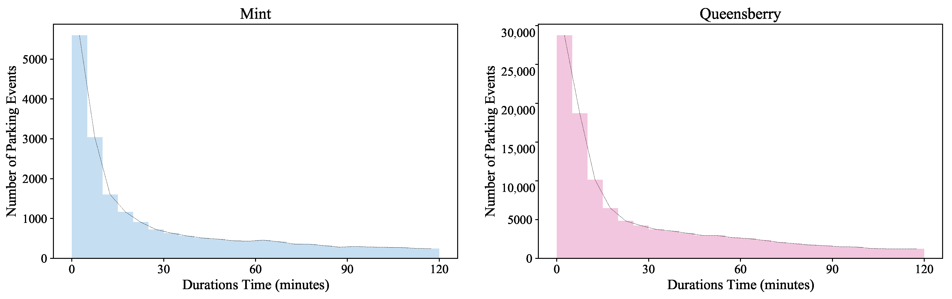
For a parking event, the parking duration can be short or long. However, for an area, the distribution of the parking durations is often exponential [6]. Figure 1 shows the distributions of parking durations in two different areas in Melbourne in July 2017, and Figure 2 shows the distributions of the parking durations in the Queensberry area in different months. We can observe that there are tiny differences in the distributions of parking durations in different areas, and there are also different distributions in different months. However, no matter how the location and time change, the distributions are all basically exponential. Therefore, we can use the probability density function of the exponential distribution, which is defined as
to approximate the distributions of the parking durations in different areas, where is a parameter of the function. The distributions of the parking durations in different areas include a long-term spatial–temporal correlation. Specifically, similarly to the POR of an area at a different sample time, the duration distributions are also temporal, and are affected by contextual spatial features, such as the distances between the two areas.
The size of parameter of the function can be used to measure the closeness of the relationship between two areas. The absolute value of the difference in two parameters is denoted as . We call this difference the “distribution distance”. Similarly to the weight matrix in Section 3.2, we can obtain another weight matrix based on the “distribution distance”. The weight based on the “distribution distance” of the i-th and j-th areas is expressed as
where is a parameter used for controlling the distribution of .
3.4. Problem Definition
Based on the definition of the graph of the POR of the areas, we predict the POR of areas in the next H time steps based on the observations in the previous M time steps. The problem can be formulated as
where and are the observation vector and the prediction vector of all of the areas at sample time t, respectively. is the conditional probability function.
4. Methodology
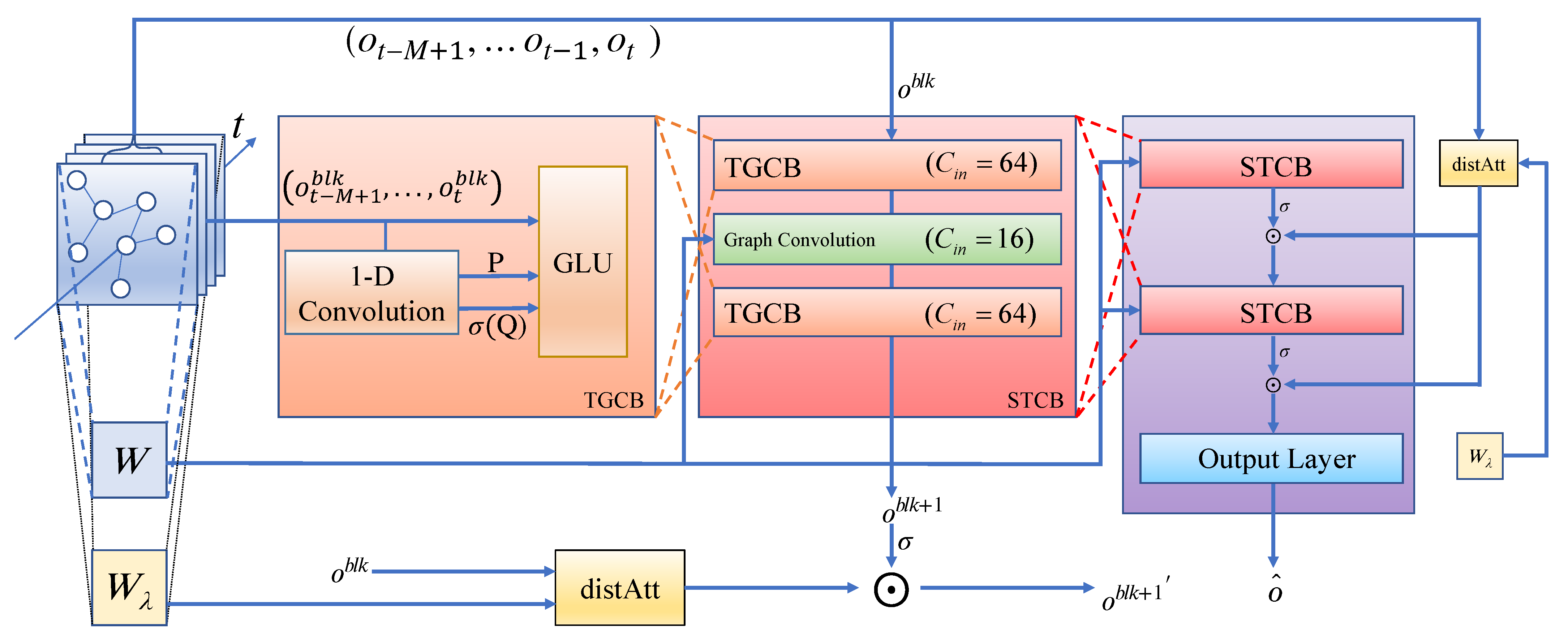
In this section, we introduce the HST-GCNs that are designed in our paper to predict the POR. As shown in Figure 3, the HST-GCN model includes three main blocks: the graph convolutional block, the temporal gated convolutional block (TGCB), and the spatial–temporal convolutional block (STCB). Each STCB includes two TGCBs together with a graph convolutional block in the middle.
4.1. Graph Convolutional Block
Since the classical CNN method cannot directly process the on-street parking data that exists in a non-Euclidean space, we use the graph constructed in Section 3.2 to extract the global contextual information of parking areas.
There are two approaches to generalizing CNNs to structured data forms. One is the spatial approach, and the other is the spectral approach. The spatial approach can be adopted on the graph by construction, which faces a great challenge when matching local neighborhoods [32]. It expands the spatial definition of convolution on the graph [33]. The latter defines a convolutional theorem based on the Fourier transform to apply the convolutions in spectral domains [32]. Moreover, we adopt an enhanced spectral method proposed by Defferrard et al. [34] to model the relationships of nearby parking areas. This enhanced spectral method reduces the evaluation complexity to linearity from and can also match local neighborhoods.
Using the spectral approach, the symmetric normalized Laplacian matrix is defined as , where is the identity matrix, W is the weight matrix defined in Section 3.2, and is the diagonal degree matrix with . As L is symmetric and positive-semidefinite, it can be expressed as , where is the diagonal matrix of eigenvalues of L, and U is the matrix made up of eigenvectors of L. The graph convolution operator is defined as
where x is the input filtered by kernel , and ⊙ is the element-wise Hadamard product. After filtering x with , the output can be expressed as
where is the kernel of the graph.
Based on Equation (6), we create the graph convolutional block to process the input of a graph. Though graphs can be processed in the spectral domain, the computational complexity is high () [32]. Furthermore, there is no spatial localization in the kernel. In other words, the kernel mentioned in Equation (5) is a global fully connected convolution kernel. In our graph convolutional block, to localize the kernel and reduce the number of parameters, a polynomial filter is applied, which is shown as
where is the coefficient of . K is the kernel size of the graph convolution, and determines the maximum radius of the convolution from the central nodes. After applying the polynomial filter, the number of parameters of the kernel is reduced from A (A is the number of areas) to K, due to which the learning complexity is also reduced from to linearity. Based on [35], the kernel can be replaced by the Chebyshev polynomials. The Chebyshev polynomials are shown as
Replacing the kernel with the Chebyshev polynomials, the kernel can be rewritten as
where is the coefficient of , is the Chebyshev polynomial of order k, and is the reshaped diagonal matrix of eigenvalues, which is expressed as . Here, is the largest eigenvalue of L. Let ; then, Equation (10) can be rewritten as
where y is the output.
Though the output can be obtained using the Chebyshev polynomials, there are still K items in Equation (11). Therefore, to further decrease the complexity, we use the 1st-order approximation [19] in our proposed model. Specifically, on the condition that the convolutional filter functions can be recovered [19], the order of the layer-wise convolution operation in Equation (10) can be limited to ; i.e., all nodes exploit the information from the (K-1)-order (1-order) neighborhoods. In this way, a linear function on the graph Laplacian spectrum can be obtained. Based on this, Equation (11) is thus approximated as
where , are two parameters of the kernel. By further assuming that , Equation (12) is simplified as
To reduce the number of parameters, let . To stabilize the numerical performances and avoid exploding/vanishing gradients, W and D are normalized by and , respectively. The output is rewritten as
By using the 1st-order approximation strategy in our graph convolutional block, the accuracy of the output is slightly reduced. However, the computational complexity has been greatly reduced, which is efficient for large-scale graphs.
4.2. Temporal Gated Convolutional Block
To extract the temporal features and capture the dynamic behavior of POR data, we construct a temporal gated convolutional block (TGCB). As Figure 3 shows, the TGCB contains a 1D CNN with a -width kernel followed by gated linear unit (GLU), which works as follows. For the entire graph, the input contains M historical observations of A nodes. The input is , where is the size of the input of the feature maps ( in this study). We use the convolutional kernels to obtain a single convolutional output result , where is the size of the feature maps generated by the GLU. and are two equal parts of the output through the 1D convolutional layer, serving as the inputs of the gates in the GLU, respectively. The temporal gated convolution is expressed as
where is the kernel of temporal convolution. Y is the input of temporal convolution. is the sigmoid function for controling . As the temporal convolution explores neighbors of input elements, it shortens the length of sequences by each time. When the input dimension is less than the output dimension, the input will be filled with enough zeros to match the length of the output. Finally, based on Equation (15) and the GLU, we create the TGCB. Differently from RNNs, which maintain a hidden state of the entire past and therefore make it difficult to perform parallel computations within a sequence, the convolutional networks in the TGCB do not depend on the computation results of previous time steps, which allows parallelization of computation during training and helps increase the computing speed.
4.3. Spatial–Temporal Convolutional Block
To combine the temporal POR data and spatial-featured graph, as shown in Figure 3 (left), we construct the Spatial–Temporal Convolutional Block (STCB) , which consists of two TGCBs and a graph convolutional block in the middle. The TGCB and the graph convolutional block are used to extract temporal correlations and spatial correlations, respectively. Let be the input of all the historical observations used for prediction; the output , which passes by one STCB , is computed as
where and are the upper and lower temporal kernels with block , is the spectral kernel of graph convolution, and ReLU (·) indicates the rectified linear unit function [36]. Following this, to achieve parallelization over input with fewer parameters and a faster training speed, a temporal convolutional layer and a fully connected layer are added to the two stacked STCBs, where the temporal convolutional layer is used to map the output. Then, we can obtain an output . Thus, the predicted value can be calculated with a linear transform through the fully connected layer.
4.4. Hybrid Spatial–Temporal Correlations
To extract both the instantaneous and the long-term spatial–temporal correlations, we consider the POR data and the distance between the areas as the first spatial–temporal relationship. The similarity of the parking duration distributions serves as the second spatial–temporal relationship. To illustrate this long-term relationship, we use the weight matrix generated by Equation (3). For the purpose of considering the two spatial–temporal correlations together, we add the weight matrix to the STCB block.
There is a long-term spatial–temporal relationship in the graph. Similarly to the distance between the areas, the similarity of parking duration distributions of the areas is also important contextual information. However, the impacts of the similarities of the parking duration distributions on areas are quite different. We adopt the idea of the graph attention networks (GATs) [26] in order to assign different levels of importance of the similarities of the parking duration distributions to different nodes within a neighborhood while dealing with neighborhoods with different distances.
Graph attention networks (GATs), which operate on graph-structured data, leverage masked self-attentional layers and can solve several challenges of spectral-based graph neural networks. The input of a GAT is a set of features of nodes, which can be denoted as , where , and is the number of features of each node. The output is also a set of features of nodes, denoted as , where , and is the number of output features of each node. We denote as the attentional featured weight matrix of all nodes. The attention coefficients are computed as
where is the attention mechanism operation function. Let be the neighbors of node i (that connect with node i directly). Then, we normalize the attention coefficients using the softmax function:
The normalized attention coefficients are used to compute a linear combination of the features corresponding to them in order to serve as the final output features for every node:
where is the activation function [26].
However, the similarity value in the GAT is not very stable, since it is learned from the attentional weight matrix and the attention function shown in Equation (17), rather than a fixed value. Motivated by the cosAtt method proposed by [29], which adopts a global GAT to learn the similar conditions of any two roads of a traffic network instead of neighbors in graph attention networks, we propose a method to measure the similarity of parking duration distributions. The method is based on the “distribution distance” mentioned in Section 3.3, in which is defined as
where is all of the nodes except node i, and is the “distribution distance” weight matrix between node i and j. The sigmoid function is the activation function, which can prevent denominator underflow and crashing of the program when the number of nodes is huge. In addition, by adopting the method, unlike the value of in GAT, the value of becomes relatively stable and is adjusted only by the weight matrix (i.e., ). Combining the output and the , we can obtain the final attentional output .
4.5. Loss Function
In this study, we use loss to measure the performance of the proposed model, which is defined as
where represents all trainable parameters, is the prediction value, and denotes the ground truth.
In this paper, the entire process of the parking occupancy prediction is illustrated by Algorithm 1.
| Algorithm 1: POR Prediction Algorithm |
Input: The arrival and departure events of the sampled parking bays and the vector of sampled time , where n is 8928; Output: The evaluation metric, i.e., the mean absolute error (MAE), root mean square error (RMSE), and mean absolute percentage error (MAPE)
|
5. Experiments
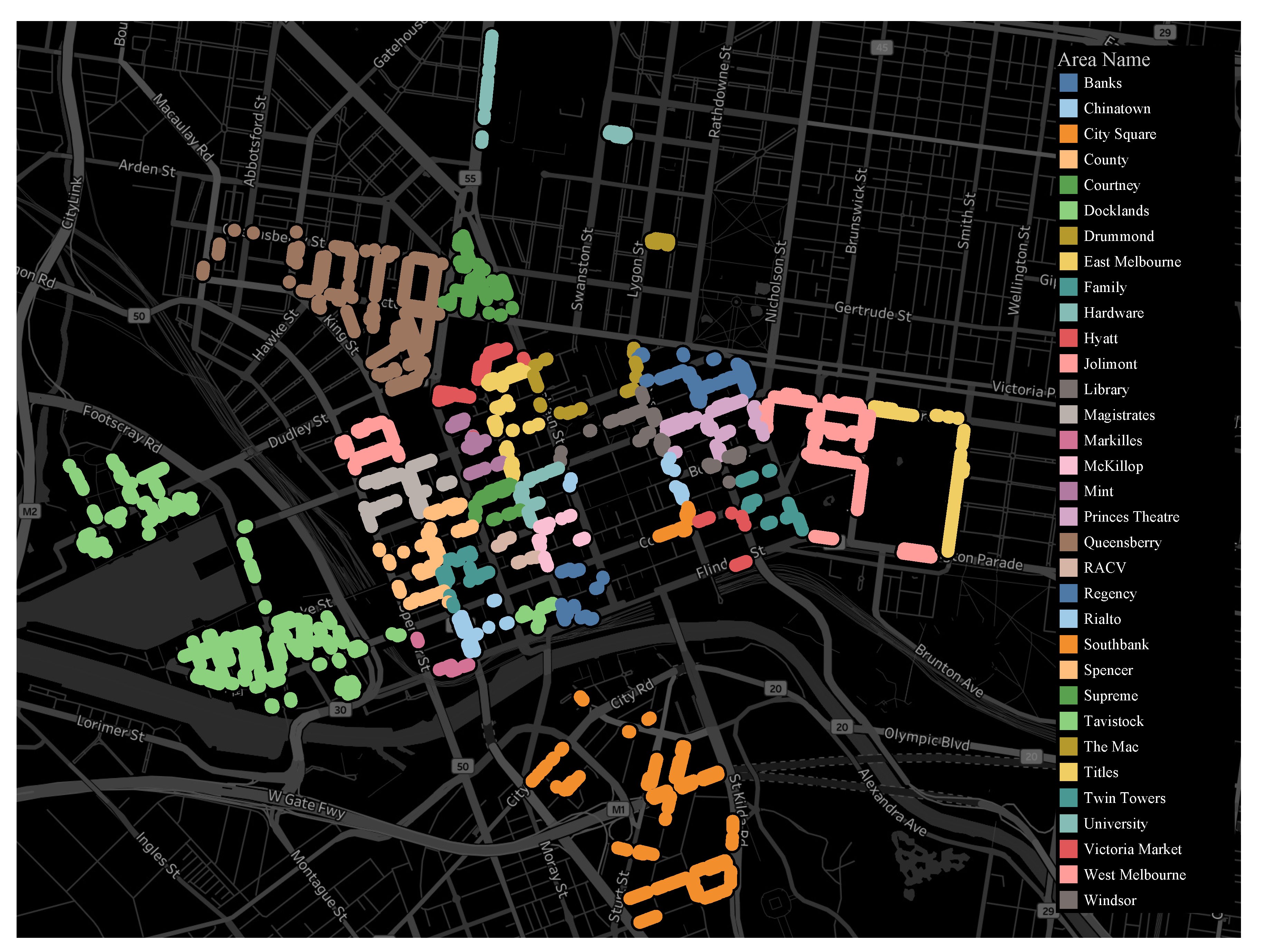
In this section, we conduct experiments to evaluate the proposed parking occupancy prediction scheme by using real-world datasets. The two datasets used in this paper are from the open data platform of Melbourne [6,37]. One dataset (dataset I) is a map indicating the positions of all 4657 parking bays and 33 areas in the city of Melbourne, as shown in Figure 4. The other dataset (dataset II) records all of the parking events of every parking bay in the city of Melbourne in 2017. In dataset II, the parking data were already influenced by many factors, such as schools, hospitals, weather, and residential areas. In other words, the parking data were influenced by the activities of all people in Melbourne. It is difficult to consider a single factor while keeping other factors constant. In addition, parking events are affected by these factors jointly. Modeling the parking events in several areas and using the datasets generated by simulations may verify the effects of a single factor on the experimental results, but they do not represent the true situation. Therefore, we considered these factors as an indivisible whole. The main features of dataset II are shown in Table 1.
5.1. Data Pre-Processing
5.1.1. Data Selection
As Figure 2 shows, the distributions of the parking durations in different months are similar. Therefore, a random selection for one month has little effect on the experimental results. In our experiments, we randomly chose one month from the raw data, which ranged from 1 July 2017 to 31 July 2017. Differently from some studies [12,24], the parking data on weekends and evenings were included.
5.1.2. On-Street Parking Occupancy Rate
According to the arrival time and departure time in each parking bay recorded in dataset II, we can obtain the parking status of each parking bay at each sample time. Then, we calculate the POR (parking occupancy rate) of each area using Equation (1). Dataset II comprises all parking events, including arrivals and departures; thus, we can accurately capture the parking state at any time. Therefore, the POR data that we calculate are always real data.
Dataset II is aggregated for every 5 min; thus, there are 288 (24 × 60 ÷ 5) time slots in every day. Correspondingly, every bay contains 288 parking occupancy rate (POR) values per day. Then, the POR can be expressed by an ordered integer , e.g., t = 00:00 as = 0 and t = 13:30 as = 162 (13 × 12 ÷ 6). All of the POR values are generated as time series.
5.1.3. The Weight Matrix
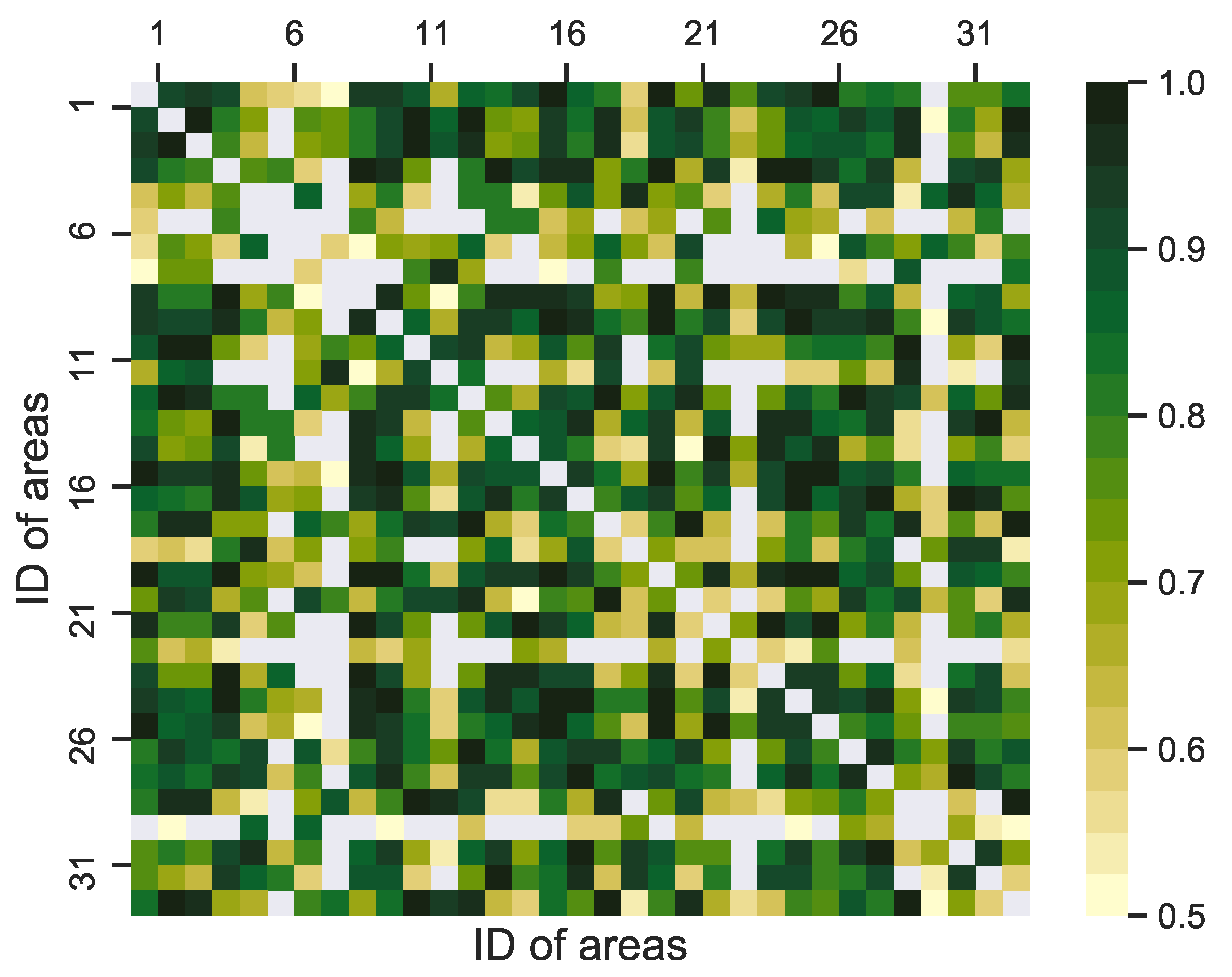
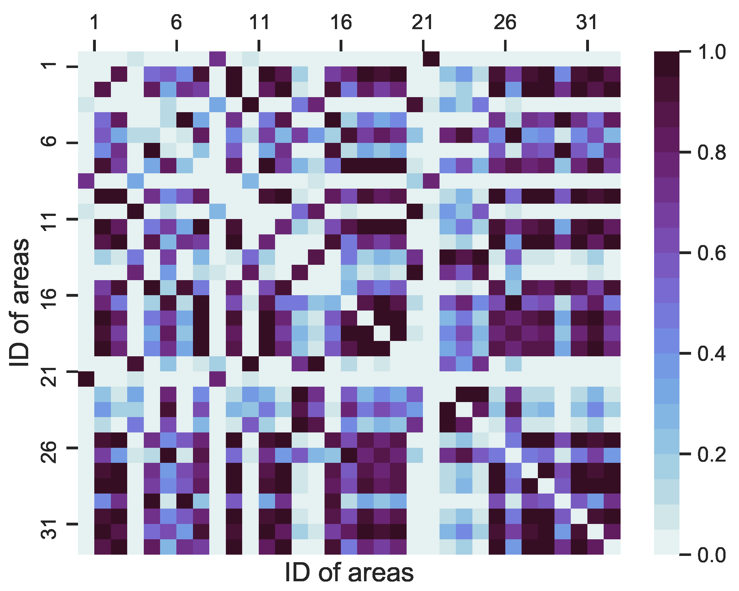
Based on the definitions of in Section 3.2, the distance weight matrix can be calculated by using Equation (2), the parameters of which are detailed as follows. and are assigned to 0.5 and 5, respectively. As for the “distribution distance” weight matrix , the parameter is set to . The visualizations of W and are shown in Figure 5 and Figure 6.
5.2. Experimental Setting
5.2.1. Evaluation Metric
To better illustrate the performance of our scheme, we use the following evaluation metrics for occupancy prediction.
- Mean absolute error (MAE):
- Root mean square error (RMSE):
- Mean absolute percentage error (MAPE):
Here, and are the actual value and the predicted value, respectively, and N is the number of samples.
5.2.2. Prediction Models
The models considered in our paper include linear models and deep learning models.
- HA: The historical average, which models the POR as a seasonal process and uses a weighted average of previous seasons as the prediction. The period used is one week, and the prediction is based on aggregated data from previous weeks. For example, the prediction at 8:00 a.m. for this Monday is the average parking occupancy rate (POR) at 8:00 a.m. on all previous Mondays. Since the historical average method does not depend on short-term data, its performance is invariant for different prediction horizons.
- ARIMA: The autoregressive integrated moving average (ARIMA) [20] model, which is also known as an integrated moving average autoregressive model, is one of the time-series forecasting analysis methods.
- LSTM: In the long short-term memory model [7], the temporal correlations are taken into account. However, the spatial correlations are not captured.
- DCRNN: The diffusion convolution recurrent neural network [17], which uses a bidirectional graph random walk to model spatial dependency and a recurrent neural network to capture the temporal dynamics.
- STGCN: The spatio-temporal graph convolutional network [18], which combines graph convolutional networks and temporal gated networks to capture spatial–temporal correlations.
- ASTGCN: The attention-based spatial–temporal graph convolution network [27], which combines the spatial–temporal attention mechanism and the spatial–temporal convolution to capture the dynamic spatial–temporal correlations.
5.2.3. Details of the Experiment
- All of the experiments were performed on a Windows 10 platform (CPU: AMD Ryzen 7 3700X 8-Core Processor @ 3.60 GHz, GPU: GeForce GTX 1650 SUPER).
- Though parking events have different characteristics between weekdays and weekends, to keep the data uniform, we considered all of July to evaluate the performance of the proposed scheme. At any sample time, all of the models used the previous 60 min (i.e., ) of observed data points to predict parking conditions in the next 15, 30, and 60 min (i.e., ).
- In the HST-GCN model, the channels of the three layers in the STCB were set to 64, 32, and 64, respectively. Furthermore, the graph convolution kernel size K and temporal convolution kernel size were set to 3.
- For the Chebyshev polynomial approximation in the proposed scheme, we trained our models by minimizing the mean square error using RMSProp [38] for 100 epochs with a batch size of 64. The initial learning rate was with a decay rate of 0.5 after every 10 epochs. The proportion of training, validation, and testing parts of the datasets were split to 23:4:4.
- To show the effects of our mechanism, we created a new model named HST-GCN , which replaced the mechanism with a GAT for comparison.
5.3. Experimental Results
The results of the prediction performance of our scheme and the benchmark models are shown in Table 2. They show that, generally speaking, the state-of-the-art deep learning performed better than the classical statistical model, i.e., the ARIMA model. Since the ARIMA and LSTM models could not capture complex spatial–temporal correlations, the two models did not perform well. As for the state-of-the-art deep learning models, they paid attention to both spatial and temporal features. However, the DCRNN model did not capture the spatial and temporal features at the same time; it performed worse than other spatial–temporal models, i.e., the STGCN, ASTGCN, and HST-GCN models.
By adding the attentional mechanism to the proposed model and using the hybrid spatial–temporal correlations, the proposed model performed better in long-term predictions. Specifically, for a 15-min horizon prediction, the RMSE of the proposed HST-GCN was the same as that of the STGCN. For a 30-min horizon prediction, HST-GCN performed 1.11% better than the STGCN model with regard to the RMSE metric. For a 60-min horizon prediction, the HST-GCN performed 2.74% better than the STGCN model with regard to the RMSE metric.
Table 3 shows the comparison of the training times between the proposed model and the state-of-the-art models. Since the STGCN and HST-GCN models use a gated 1D CNN, which supports massive parallel computing to extract temporal features, the training time was much shorter. Specifically, the two models were 4.16 times faster than the ASTGCN model and 41.2 times faster than the DCRNN model.
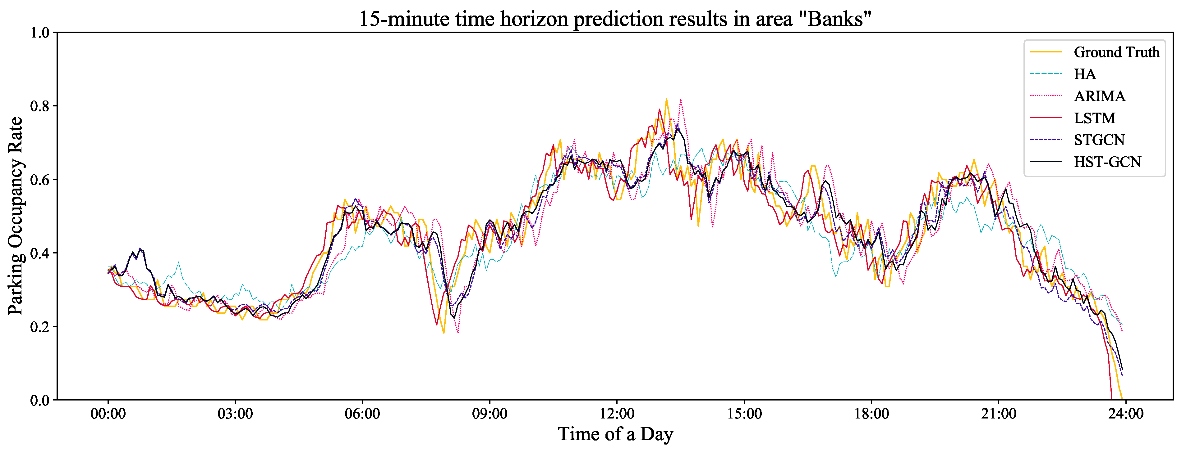
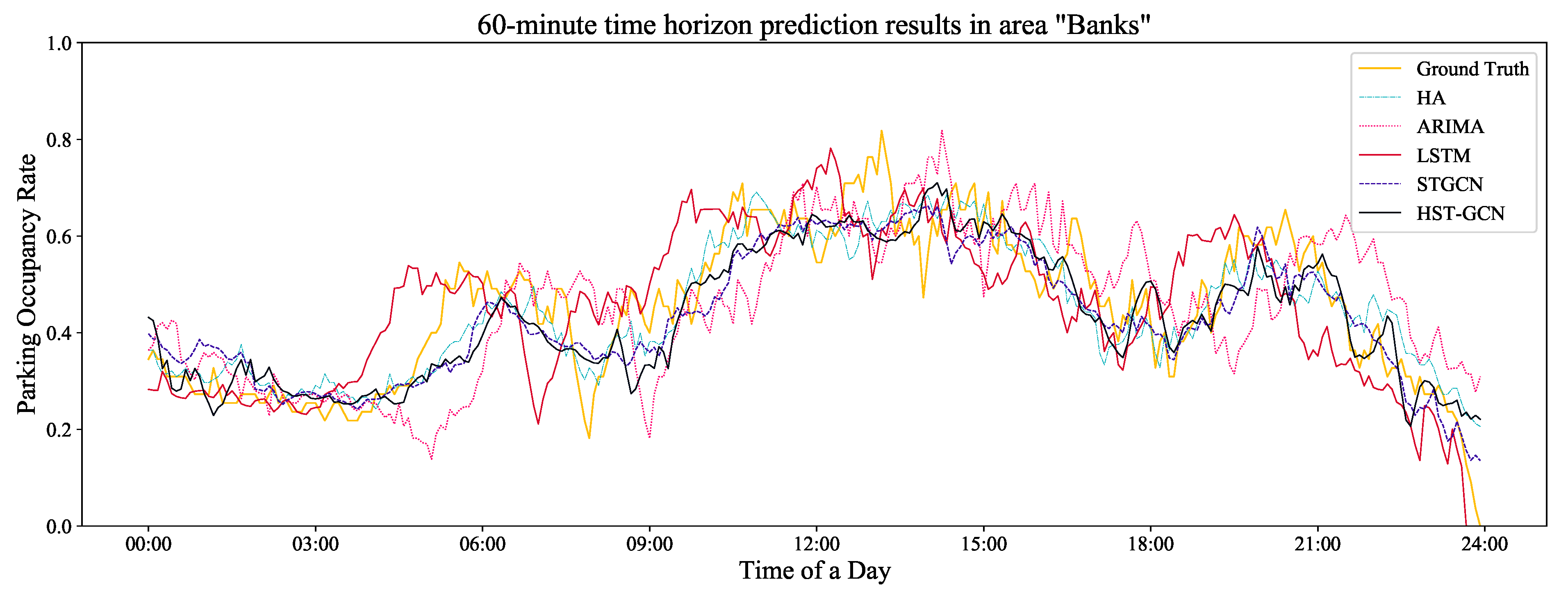
To better illustrate the performance of the benchmark models and the proposed model, we also randomly selected one area (e.g., “Banks”) and used the real observation data (i.e., the ground truth) of this area for a comparison. The comparison results are shown in Figure 7, Figure 8 and Figure 9. Obviously, there were time lags in the ARIMA model. For the STGCN and LSTM models, the prediction results fluctuated greatly over time. In addition, it can be seen from these figures that the prediction results of the three models above were also greatly affected by the lengths of the prediction horizons. The shorter the time horizon was, the better the prediction results were. For the proposed HST-GCN model, the figures show that the prediction results were approximately consistent with the real values.
Table 4 shows the results of the POR predictions of the HST-GCN and HST-GCN* (replace with GAT). Both of the models were trained 10 times with the same hyperparameters. The results show that by using the method, we can obtain a more stable prediction value.
6. Conclusions and Future Work
In this paper, we proposed the hybrid spatial–temporal graph convolutional network (HST-GCN) model for on-street parking space prediction with a large number of real-world datasets. Specifically, we captured instantaneous spatial–temporal correlations by using gated temporal convolution and graph convolution. We also proposed an attention mechanism called together with a spatial–temporal convolutional block to mix the long-term spatial–temporal correlations and instantaneous spatial–temporal correlations. Based on real-world datasets, the experimental results showed that the proposed scheme performed better than the baseline models in predicting the parking occupancy rate (POR). The HST-GCN model can be used for many other scenes of static activities. For example, it may be used to count the number of people in a library, as people may stay for a long time to read in the library. However, this model is not suitable for dynamic activities with rapid location changes, such as for predicting traffic flows. Furthermore, in each area, the inner spatial features of sub-geographies, i.e., the interactions between parking bays within an area, are also points of interest that are worth discussing. In the future, we plan to use our proposed model for other new scenes with more datasets in different places while considering more factors that may influence the prediction results, such as the weather and schools.
Author Contributions
Conceptualization, X.X. and Z.J.; methodology, X.X. and Z.J.; resources, W.S.; experiment, Z.J.; writing—original draft preparation, Z.J.; writing—review and editing, Y.X., Z.J. and X.X.; visualization, Y.H.; supervision, X.X. and W.S. All authors have read and agreed to the published version of the manuscript.
Funding
This work was supported in part by the National Key R&D Program of China under Grant 2019YFB1600100, in part by the NSFC under Grant 61901341, in part by the China Postdoctoral Science Foundation under Grant 2021TQ0260, in part by the XAST under Grant 095920201322, in part by the National Natural Science Foundation of Shaanxi Province under Grant 2020JQ-301, and in part by the Fundamental Research Funds for the Central Universities of Ministry of Education of China under Grant XJS200109.
Data Availability Statement
The datasets used in this study were all downloaded from the Melbourne open data platform. The dataset of on-street parking events in 2017 is available at https://data.melbourne.vic.gov.au/Transport/On-street-Car-Parking-Sensor-Data-2017/u9sa-j86i (accessed on 27 May 2021), and the map data of Melbourne on-street parking bays is available at https://data.melbourne.vic.gov.au/Transport/On-street-Parking-Bays/crvt-b4kt (accessed on 13 December 2020).
Acknowledgments
The authors would like to thank Xinrui Ma for critically reviewing the manuscript. The experiments were performed at the Deep Intelligence Laboratory of Xidian University. The people involved in the laboratory are gratefully acknowledged for their help.
Conflicts of Interest
The authors declare no conflict of interest.
References
- Manville, M.; Shoup, D. People, Parking and Cities. J. Urban Plan. Dev. 2005, 131, 233–245. [Google Scholar] [CrossRef] [Green Version]
- Lin, T.; Rivano, H.; Le Mouël, F. A Survey of Smart Parking Solutions. IEEE Trans. Intell. Transp. Syst. 2017, 18, 3229–3253. [Google Scholar] [CrossRef] [Green Version]
- Gallivan, S. IBM Global Parking Survey: Drivers Share Worldwide Parking Woes; Technical Report; IBM: New York, NY, USA, 2011. [Google Scholar]
- Bock, F.; Di Martino, S.; Origlia, A. Smart Parking: Using a Crowd of Taxis to Sense On-Street Parking Space Availability. IEEE Trans. Intell. Transp. Syst. 2020, 21, 496–508. [Google Scholar] [CrossRef]
- Tilahun, S.L.; Di Marzo Serugendo, G. Cooperative multiagent system for parking availability prediction based on time varying dynamic Markov chains. J. Adv. Transp. 2017, 2017, 1760842. [Google Scholar] [CrossRef]
- Shao, W.; Salim, F.D.; Gu, T.; Dinh, N.T.; Chan, J. Traveling Officer Problem: Managing Car Parking Violations Efficiently Using Sensor Data. IEEE Internet Things J. 2018, 5, 802–810. [Google Scholar] [CrossRef]
- Shao, W.; Tan, S.; Zhao, S.; Qin, K.K.; Hei, X.; Chan, J.; Salim, F.D. Incorporating LSTM Auto-Encoders in Optimizations to Solve Parking Officer Patrolling Problem. ACM Trans. Spat. Algorithms Syst. (TSAS) 2020, 6, 1–21. [Google Scholar] [CrossRef]
- Guo, J.; He, H.; Sun, C. ARIMA-Based Road Gradient and Vehicle Velocity Prediction for Hybrid Electric Vehicle Energy Management. IEEE Trans. Veh. Technol. 2019, 68, 5309–5320. [Google Scholar] [CrossRef]
- Zhang, X.; Zhao, Z.; Zheng, Y.; Li, J. Prediction of Taxi Destinations Using a Novel Data Embedding Method and Ensemble Learning. IEEE Trans. Intell. Transp. Syst. 2020, 21, 68–78. [Google Scholar] [CrossRef]
- Luo, X.; Li, D.; Yang, Y.; Zhang, S. Spatiotemporal traffic flow prediction with KNN and LSTM. J. Adv. Transp. 2019, 2019. [Google Scholar] [CrossRef] [Green Version]
- Du, B.; Peng, H.; Wang, S.; Bhuiyan, M.Z.A.; Wang, L.; Gong, Q.; Liu, L.; Li, J. Deep Irregular Convolutional Residual LSTM for Urban Traffic Passenger Flows Prediction. IEEE Trans. Intell. Transp. Syst. 2020, 21, 972–985. [Google Scholar] [CrossRef]
- Shao, W.; Zhang, Y.; Guo, B.; Qin, K.; Chan, J.; Salim, F.D. Parking Availability Prediction with Long Short Term Memory Model. In Green, Pervasive, and Cloud Computing; Li, S., Ed.; Springer International Publishing: Berlin/Heidelberg, Germany, 2019; pp. 124–137. [Google Scholar]
- Vu, H.T.; Huang, C.C. Parking Space Status Inference Upon a Deep CNN and Multi-Task Contrastive Network with Spatial Transform. IEEE Trans. Circuits Syst. Video Technol. 2019, 29, 1194–1208. [Google Scholar] [CrossRef]
- Chandra, R.; Bhattacharya, U.; Bera, A.; Manocha, D. Traphic: Trajectory Prediction in Dense and Heterogeneous Traffic Using Weighted Interactions. In Proceedings of the IEEE Conference on Computer Vision and Pattern Recognition, Long Beach, CA, USA, 15–20 June 2019; pp. 8483–8492. [Google Scholar]
- Zhao, L.; Song, Y.; Zhang, C.; Liu, Y.; Wang, P.; Lin, T.; Deng, M.; Li, H. T-GCN: A Temporal Graph Convolutional Network for Traffic Prediction. IEEE Trans. Intell. Transp. Syst. 2019, 21, 3848–3858. [Google Scholar] [CrossRef] [Green Version]
- Li, Z.; Xiong, G.; Chen, Y.; Lv, Y.; Hu, B.; Zhu, F.; Wang, F.Y. A Hybrid Deep Learning Approach with GCN and LSTM for Traffic Flow Prediction. In Proceedings of the 2019 IEEE Intelligent Transportation Systems Conference (ITSC), Auckland, New Zealand, 27–30 October 2019; pp. 1929–1933. [Google Scholar]
- Li, Y.; Yu, R.; Shahabi, C.; Liu, Y. Diffusion Convolutional Recurrent Neural Network: Data-Driven Traffic Forecasting. arXiv 2018, arXiv:1707.01926. [Google Scholar]
- Yu, B.; Yin, H.; Zhu, Z. Spatio-Temporal Graph Convolutional Networks: A Deep Learning Framework for Traffic Forecasting. In Proceedings of the 27th International Joint Conference on Artificial Intelligence, Stockholm, Sweden, 13–19 July 2018; pp. 3634–3640. [Google Scholar]
- Kipf, T.N.; Welling, M. Semi-Supervised Classification with Graph Convolutional Networks. arXiv 2016, arXiv:1609.02907. [Google Scholar]
- Yu, F.; Guo, J.; Zhu, X.; Shi, G. Real time prediction of unoccupied parking space using time series model. In Proceedings of the 2015 International Conference on Transportation Information and Safety (ICTIS), Wuhan, China, 25–28 June 2015; pp. 370–374. [Google Scholar] [CrossRef]
- Liu, Y.; Sha, M. Research on Prediction of Traffic Flow at Non-detector Intersections Based on Ridge Trace and Fuzzy Linear Regression Analysis. In Proceedings of the 2009 International Conference on Computational Intelligence and Security, Beijing, China, 11–14 December 2009; Volume 2, pp. 571–575. [Google Scholar]
- Bock, F.; Di Martino, S.; Origlia, A. A 2-step approach to improve data-driven parking availability predictions. In Proceedings of the 10th ACM SIGSPATIAL Workshop on Computational Transportation Science, Redondo Beach, CA, USA, 7–10 November 2017; pp. 13–18. [Google Scholar]
- Vlahogianni, E.I.; Kepaptsoglou, K.; Tsetsos, V.; Karlaftis, M.G. A Real-Time Parking Prediction System for Smart Cities. J. Intell. Transp. Syst. 2016, 20, 192–204. [Google Scholar] [CrossRef]
- Zheng, Y.; Rajasegarar, S.; Leckie, C. Parking Availability Prediction for Sensor-Enabled Car Parks in Smart Cities. In Proceedings of the 2015 IEEE Tenth International Conference on Intelligent Sensors, Sensor Networks and Information Processing (ISSNIP), Singapore, 7–9 April 2015; pp. 1–6. [Google Scholar]
- Yang, S.; Ma, W.; Pi, X.; Qian, S. A Deep Learning Approach to Real-Time Parking Occupancy Prediction in Transportation Networks Incorporating Multiple Spatio-Temporal Data Sources. Transp. Res. Part C Emerg. Technol. 2019, 107, 248–265. [Google Scholar] [CrossRef]
- Veličković, P.; Cucurull, G.; Casanova, A.; Romero, A.; Liò, P.; Bengio, Y. Graph Attention Networks. In Proceedings of the International Conference on Learning Representations, Vancouver, BC, Canada, 30 April–3 May 2018. [Google Scholar]
- Guo, S.; Lin, Y.; Feng, N.; Song, C.; Wan, H. Attention Based Spatial-Temporal Graph Convolutional Networks for Traffic Flow Forecasting. In Proceedings of the AAAI Conference on Artificial Intelligence, Honolulu, HI, USA, 27 January–1 February 2019; Volume 33, pp. 922–929. [Google Scholar] [CrossRef] [Green Version]
- Zheng, C.; Fan, X.; Wang, C.; Qi, J. GMAN: A Graph Multi-Attention Network for Traffic Prediction. In Proceedings of the AAAI Conference on Artificial Intelligence, New York, NY, USA, 7–8 February 2020; Volume 34, pp. 1234–1241. [Google Scholar]
- Huang, R.; Huang, C.; Liu, Y.; Dai, G.; Kong, W. LSGCN: Long Short-Term Traffic Prediction with Graph Convolutional Networks. In Proceedings of the Twenty-Ninth International Joint Conference on Artificial Intelligence (IJCAI-20), Yokohama, Japan, 11–17 July 2020; Bessiere, C., Ed.; International Joint Conferences on Artificial Intelligence Organization, 2020; pp. 2355–2361. [Google Scholar]
- Shao, W.; Zhao, S.; Zhang, Z.; Wang, S.; Rahaman, M.S.; Song, A.; Salim, F.D. FADACS: A Few-Shot Adversarial Domain Adaptation Architecture for Context-Aware Parking Availability Sensing. In Proceedings of the 2021 IEEE International Conference on Pervasive Computing and Communications (PerCom), Pisa, Italy, 21–25 March 2021; pp. 1–10. [Google Scholar] [CrossRef]
- Liu, K.S.; Gao, J.; Wu, X.; Lin, S. On-Street Parking Guidance with Real-Time Sensing Data for Smart Cities. In Proceedings of the 2018 15th Annual IEEE International Conference on Sensing, Communication, and Networking (SECON), Hong Kong, China, 11–13 June 2018; pp. 1–9. [Google Scholar]
- Bruna, J.; Zaremba, W.; Szlam, A.; LeCun, Y. Spectral Networks and Locally Connected Networks on Graphs. arXiv 2013, arXiv:1312.6203. [Google Scholar]
- Niepert, M.; Ahmed, M.; Kutzkov, K. Learning convolutional Neural Networks for Graphs. In Proceedings of the International Conference on Machine Learning (PMLR), New York, NY, USA, 20–22 June 2016; pp. 2014–2023. [Google Scholar]
- Defferrard, M.; Bresson, X.; Vandergheynst, P. Convolutional Neural Networks on Graphs with Fast Localized Spectral Filtering. In Proceedings of the 30th International Conference on Neural Information Processing Systems (NIPS’16), Barcelona, Spain, 4–9 December 2016; Curran Associates Inc.: Red Hook, NY, USA, 2016; pp. 3844–3852. [Google Scholar]
- Chatterjee, S.; Roy, S.; Das, A.K.; Chattopadhyay, S.; Kumar, N.; Vasilakos, A.V. Secure Biometric-Based Authentication Scheme Using Chebyshev Chaotic Map for Multi-Server Environment. IEEE Trans. Dependable Secur. Comput. 2016, 15, 824–839. [Google Scholar] [CrossRef]
- Wang, G.; Giannakis, G.B.; Chen, J. Learning ReLU Networks on Linearly Separable Data: Algorithm, Optimality, and Generalization. IEEE Trans. Signal Process. 2019, 67, 2357–2370. [Google Scholar] [CrossRef] [Green Version]
- Shao, W.; Salim, F.D.; Song, A.; Bouguettaya, A. Clustering Big Spatiotemporal-Interval Data. IEEE Trans. Big Data 2016, 2, 190–203. [Google Scholar] [CrossRef]
- Dubey, S.R.; Chakraborty, S.; Roy, S.K.; Mukherjee, S.; Singh, S.K.; Chaudhuri, B.B. DiffGrad: An Optimization Method for Convolutional Neural Networks. IEEE Trans. Neural Netw. Learn. Syst. 2020, 31, 4500–4511. [Google Scholar] [CrossRef] [PubMed] [Green Version]
Figure 1.
The distributions of the parking durations in two different areas (Mint and Queensberry) in Melbourne in July 2017.
Figure 1.
The distributions of the parking durations in two different areas (Mint and Queensberry) in Melbourne in July 2017.

Figure 2.
The distributions of the parking durations in the Queensberry area in Melbourne in each month of 2017.
Figure 2.
The distributions of the parking durations in the Queensberry area in Melbourne in each month of 2017.

Figure 3.
The framework of the proposed HST-GCN model. ⊙ refers to the element-wise Hadamard product and refers to the sigmoid function.
Figure 3.
The framework of the proposed HST-GCN model. ⊙ refers to the element-wise Hadamard product and refers to the sigmoid function.

Figure 4.
A map of the distribution of parking bays and areas in Melbourne.

Figure 5.
The heat map of the visualization of the weighted matrix W, which is determined by the distance between the two areas. The color of the heat map indicates the weight values of the two parking areas, which can be calculated by using Equation (2).
Figure 5.
The heat map of the visualization of the weighted matrix W, which is determined by the distance between the two areas. The color of the heat map indicates the weight values of the two parking areas, which can be calculated by using Equation (2).

Figure 6.
The heat map of the visualization of the weighted matrix , which is determined by the “distribution distance” between the two areas. The color of the heat map indicates the weight values of the two parking areas, which can be calculated by using Equation (3).
Figure 6.
The heat map of the visualization of the weighted matrix , which is determined by the “distribution distance” between the two areas. The color of the heat map indicates the weight values of the two parking areas, which can be calculated by using Equation (3).

Figure 7.
The prediction of a randomly selected area with a 15-min time horizon.

Figure 8.
The prediction of a randomly selected area with a 30-min time horizon.

Figure 9.
The prediction of a randomly selected area with a 60-min time horizon.


Table 1.
Features of the Melbourne parking bay dataset (dataset II).
| Feature | Description |
|---|---|
| Area | City area—used for administrative purposes. |
| ArriveTime | Date and time that the sensor detected that a vehicle was located over it. |
| DepartureTime | Date and time that the sensor detected that a vehicle was no longer located over it. |
| StreetMarker | The street marker that was located next to the parking bay with a unique ID for the bay. |
| DurationSeconds | Time difference between arrival and departure events (measured in seconds). |
| Vehicle Present | Representing whether there was a vehicle present. |
| Longitude | Geographical information |
| latitude | Geographical information |
Table 2.
Performance comparison of different models.
| Model | Evaluation Metrics (15/30/60 min) | ||
|---|---|---|---|
| MAPE (%) | MAE | RMSE | |
| HA | 15.2083 | 0.0723 | 0.0991 |
| ARIMA | 10.4794/ 13.5052/ 19.1953 | 0.0544/ 0.0696/ 0.0982 | 0.0711/ 0.0906/ 0.1236 |
| LSTM | 10.5566/ 12.9892/ 17.5452 | 0.0644/ 0.0769/ 0.1004 | 0.0886/ 0.1037/ 0.1329 |
| DCRNN | 10.4845/ 14.3646/ 19.4344 | 0.0355/ 0.0471/ 0.0649 | 0.0519/ 0.0666/ 0.0899 |
| STGCN | 7.2983/ 9.7159/ 12.9341 | 0.0355/ 0.0467/ 0.0630 | 0.0494/ 0.0639/ 0.0851 |
| ASTGCN | 9.9607/ 13.3459/ 19.2274 | 0.0351/ 0.0466/ 0.0627 | 0.0518/ 0.0665/ 0.0858 |
| HST-GCN | 7.1222/ 9.3659/ 12.2568 | 0.0345/ 0.0456/ 0.0593 | 0.0487/ 0.0632/ 0.0801 |
Table 3.
Training time consumption.
| Training Time Consumption (s) | |||
|---|---|---|---|
| STGCN | DCRNN | ASTGCN | HST-GCN |
| 151.83 | 6271.34 | 632.77 | 152.05 |
Table 4.
Prediction value changes with the method (“*” indicates that the model did not use the mechanism).
Table 4.
Prediction value changes with the method (“*” indicates that the model did not use the mechanism).
| min | MAE | MAPE (%) | RMSE | |
|---|---|---|---|---|
| HST-GCN * | 15 | 0.03496 ± 0.00031 | 7.1691 ± 0.1130 | 0.04911 ± 0.00041 |
| 30 | 0.04600 ± 0.00077 | 9.4814 ± 0.2830 | 0.06316 ± 0.00098 | |
| 60 | 0.06048 ± 0.00150 | 12.7821 ± 0.3502 | 0.08138 ± 0.00178 | |
| HST-GCN | 15 | 0.03503 ± 0.00020 | 7.1441 ± 0.0789 | 0.04916 ± 0.00033 |
| 30 | 0.04592 ± 0.00083 | 9.4658 ± 0.2778 | 0.06316 ± 0.00090 | |
| 60 | 0.06033 ± 0.00097 | 12.4288 ± 0.2719 | 0.08172 ± 0.00134 |
Publisher’s Note: MDPI stays neutral with regard to jurisdictional claims in published maps and institutional affiliations. |
© 2021 by the authors. Licensee MDPI, Basel, Switzerland. This article is an open access article distributed under the terms and conditions of the Creative Commons Attribution (CC BY) license (https://creativecommons.org/licenses/by/4.0/).
Share and Cite
MDPI and ACS Style
Xiao, X.; Jin, Z.; Hui, Y.; Xu, Y.; Shao, W. Hybrid Spatial–Temporal Graph Convolutional Networks for On-Street Parking Availability Prediction. Remote Sens. 2021, 13, 3338. https://0-doi-org.brum.beds.ac.uk/10.3390/rs13163338
AMA Style
Xiao X, Jin Z, Hui Y, Xu Y, Shao W. Hybrid Spatial–Temporal Graph Convolutional Networks for On-Street Parking Availability Prediction. Remote Sensing. 2021; 13(16):3338. https://0-doi-org.brum.beds.ac.uk/10.3390/rs13163338
Chicago/Turabian StyleXiao, Xiao, Zhiling Jin, Yilong Hui, Yueshen Xu, and Wei Shao. 2021. "Hybrid Spatial–Temporal Graph Convolutional Networks for On-Street Parking Availability Prediction" Remote Sensing 13, no. 16: 3338. https://0-doi-org.brum.beds.ac.uk/10.3390/rs13163338
Note that from the first issue of 2016, this journal uses article numbers instead of page numbers. See further details here.