Urban Growth Derived from Landsat Time Series Using Harmonic Analysis: A Case Study in South England with High Levels of Cloud Cover

Abstract

Accurate detection of spatial patterns of urban growth is crucial to the analysis of urban growth processes. A common practice is to use post-classification change analysis, overlaying multiple independently derived land cover layers. This approach is problematic as propagation of classification errors can lead to overestimation of change by an order of magnitude. This paper contributes to the growing literature on change classification using pixel-based time series analysis. In particular, we have developed a method that identifies change in the urban fabric at the pixel level based on breaks in the seasonal and year-on-year trend of the normalised difference vegetation index (NDVI). The method is applied to a case study area in the south of England that is characterised by high levels of cloud cover. The study uses the Landsat data archive over the period 1984–2018. The performance of the method was assessed using 500 ground truth points. These points were randomly selected and manually assessed for change using high-resolution earth observation imagery. The method identifies pixels where a land cover change occurred with a user’s accuracy of change 45.3 ± 4.45% and outperforms a post-classification analysis of an otherwise more advanced land cover product, which achieved a user’s accuracy of 17.8 ± 3.42%. This method performs better where changes exhibit large differences in NDVI dynamics amongst land cover types, such as the transition from agricultural to suburban, and less so where small differences of NDVI are observed, such as changes in land cover within pixels that are densely built up already. The method proved relatively robust for outliers and missing data, for example, in the case of high levels of cloud cover, but does rely on a period of data availability before and after the change event. Future developments to improve the method are to incorporate spectral information other than NDVI and to consider multiple change events per pixel over the analysed period.

1. Introduction

Global urbanisation and population growth puts pressure on environmental systems, but also provides opportunities for development [1]. The detection, classification, and characterisation of urban growth patterns is crucial to the effective management of urbanisation pressures [2]. Currently, the land cover products that are most readily available for urban analysis are ill-suited for change analysis because of error propagation. Errors in classification of earth observation imagery that are normally expected [3] can propagate and dramatically affect the analysis of change over time [4], aggravating problems of error that already exist in multi-date landscape pattern comparison [5].

A common approach to land cover change is post-classification comparison (PCC). In this approach, land cover classifications are produced independently for the same study area for two or more moments in time. Differences between the layers are then interpreted as change over time [6]. This approach is problematic, because it means that misclassifications are likely to be registered as a change. When a relatively small proportion of the study area changes over time, as is often the case, then even highly accurate classifications can lead to substantial error in the change estimates. Some of this error may be mitigated by a process of temporal filtering. This method is applied at the pixel level and identifies the change trajectory (or life-history) from multi-temporal land cover classifications. Rule-based corrections are then made based on assumptions of transition likelihood (e.g., assuming urban growth is irreversible) [7,8,9]. This process may reduce misclassification error but only for those misclassifications identified by the ruleset; other misclassifications which appear as allowed transition types may be missed. Finally, real transitions can be erroneously removed when they are deemed to be unlikely; therefore, bias may be introduced into the analysis. Pre-classification change detection techniques have been developed in response to the problems of PCC. These approaches use multitemporal, unclassified data to identify where changes take place and the nature of the change that occurred [10]. Pre-classification methods are by their multitemporal nature more complex than post-classification methods: even without land cover change, spectral signatures will vary considerably in space and over time; the challenge, then, is to identify within the highly variable data which variations indicate a land cover change [6]. Numerous pre-classification change detection methods exist, such as NDVI trajectory analysis [11], NDVI differencing [12], time series break-point analysis [13], and continuous change detection analysis [14].

This paper builds on the method introduced by Zhu and Woodcock [14], which applies harmonic analysis to the normalised difference vegetation index (NDVI), a widely used vegetation index calculated from the red and near-infrared spectral bands [15]. A low level or absence of vegetation is a defining characteristic of urban areas which therefore exhibit low NDVI values and intra-annual (seasonal) variation [9]. Rural areas are characterised by higher proportions of vegetation undergoing marked growth cycles, therefore exhibiting either higher NDVI values or larger seasonal variations of NDVI [16]. Sufficiently large deviations from established of NDVI temporal dynamics may be an indication of change [12].

The NDVI of a pixel fluctuates naturally over time both seasonally and through a year-on-year trend. The signal can therefore be modelled using a harmonic analysis, e.g., a sinusoidal function with a period of one year to reflect seasonal variation, and a linear trend to reflect year-on-year growth [14,16]. Harmonic analysis is widely used for the detection of cycles in data [17]. Theoretically, there is no limit to the number of sinusoidal components to model a time series; pragmatically, however, researchers use only a few [18].

Previously, Zhu and Woodcock [14], estimated a harmonic model for each pixel and identified a land cover change where new observations deviated from the estimated model beyond a given tolerance for three consecutive cloud-free observations. Zhu et al. [19] applied a similar method with a lower threshold for identifying change, but a requirement for a longer sustained deviation. In this article, we are concerned with change of land cover due to urbanisation in an area prone to cloud cover and will expand on the methods considering associated assumptions. We are assuming that land cover change is infrequent and irreversible and will therefore not attempt to identify more than one change event per pixel. We also intend to be robust under frequent cloud cover, which means that pixel observations may be obtained at irregular time intervals. The proposed method is therefore based on separately fitted sinusoidal functions for the period before and after a potential change event. A change event is detected when the fit (root mean squared error, RMSE) for the two separate models outperforms that of a single model for the whole period by a given threshold. The timing of change for a pixel is determined by the best fit (lowest RMSE) for the combined before and after models.

This article presents the method and its application to a case study area in southern England using the full time series of Landsat data from 1984 to 2018. Landsat data were selected for this study despite their relatively coarse resolution (30 m pixels), which cannot accurately outline many features in urban landscapes. They are used because of their universal availability and their long historical archive; a long-time record is crucial for analysis of urban change processes that have characteristic temporal scales in the order of decades. The accuracy is assessed using a dense set of ground truth pixels and their performance is compared to a PCC of existing UK land cover products.

2. Study Area

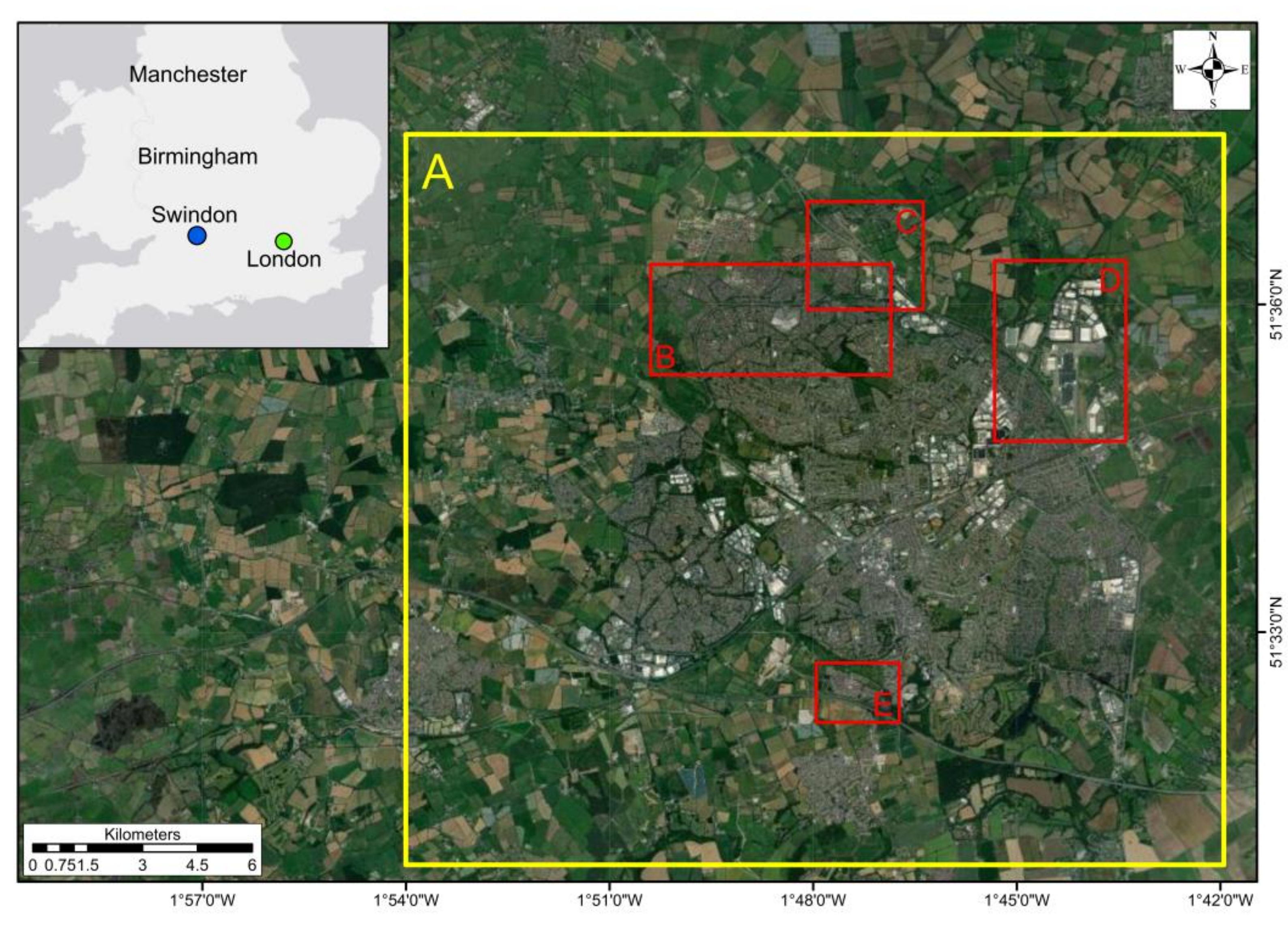
The study area consists of the town of Swindon and its surrounding area (Figure 1). Swindon is in the south-west of England and has undergone substantial urban development in the last century [20,21]. Swindon has a population of approximately 175,000 and has undergone recent, rapid growth and has a history of flooding [22]. During the mid-20th century, Swindon relied on railway-related activities yet by 1986 this was superseded by the automotive, IT, and services sectors [23]. Swindon has received investment from Honda which developed the South Marston industrial complex in 2001 [24]. This new source of employment may have provided the catalyst for further suburban development in the Hayden Wick area and facilitated a total population increase of 4.9% between 2001 and 2007 [23]. The town is surrounded by agricultural land and is not constrained by greenbelt policies. The town has seen substantial impervious surface growth [25].

3. Materials and Methods

3.1. Landsat Data

This study uses the Landsat archive [26], available through Google Earth Engine [27], for the period from 1984 to 2018. This dataset includes images acquired by Landsat Thematic Mapper (Landsat 5), Enhanced Thematic Mapper Plus (Landsat 7), and Operational Land Imager (Landsat 8). This study used tier 1 surface reflectance data which have been atmospherically corrected using the Landsat Ecosystem Disturbance Adaptive Processing System (LEDAPS), and include a cloud, shadow, water, and snow mask identified using the CFMask algorithm [28,29,30,31]. The dataset for the whole study area consists of 760 Landsat images. Over half of all pixels were masked out due to the presence of clouds and shadows as indicated by a pixel quality band generated by the CFMask algorithm [31]. Any pixel in any image which was identified by the CFMask as being contaminated with clouds, shadow, water, or snow, was removed from the analysis; however, corresponding pixels in other images remained in the analysis if they were identified as cloud-free. The red and near-infrared bands, which have a spatial resolution of 30 m, were used to calculate the NDVI [32]. In this study, no harmonisation between Landsat sensors was performed as during preliminary analysis, the NDVI calculated from surface reflectance images was observed to have a negligible impact on long-term average trends (the NDVI linear trend and amplitude, calculated below).

3.2. Ground Truth Data

Five sets of pixels were randomly and independently selected, prior to manual interpretation using high-resolution imagery from Google Earth Pro [33]. Google Earth images represent the highest resolution source of ground truth data available to this study; whilst site visits would likely yield higher quality data, the retrospective nature of this study made this impossible [34]. The availability of images for this area is not uniform, whereby the western half of the study area has a denser coverage. The whole study area is covered by images from 2002, 2003, 2005, 2012 and 2017 (

Table 1. Date of acquisition of high-resolution ground truth data covering Swindon between 1999 and 2017, and their respective coverage.

Area	Date of Acquisition
Whole study area	31 December 2002, 21 October 2003, 12 September 2005, 1 April 2012, 28 May 2012, 18 April 2017
Majority of area	31 December 1999, 13 March 2007
East	31 December 2005, 31 December 2007
West	31 December 2006, 24 March 2009, 16 March 2014, 15 April 2014, 13 March 2017
North	30 June 2003, 2 June 2009
South	9 April 2015, 14 April 2015, 18 April 2015

). The high-resolution images are of varying spatial resolution and quality, resulting in differences in ease of interpretation. Georeferencing errors are generally small (<10 m) between images; however, 12 September 2005 is shifted ~30 m west relative to others, and the images acquired on 21 October 2003 and 24 March 2009 are contaminated by cloud cover. Due to the imprecise match of high-resolution imagery and the time periods of analysis, only images within one year of the individual period of analysis were used, where required, as ground truth data. Therefore, 1999 and 2017 imagery were deemed unsuitable for any analysis.

Each selected pixel was manually classified into five land cover classes: sparsely built-up, densely built-up, bare surface, vegetation, and vegetated with minor structures (

Table 2. Land cover classes used in the study.

Land Cover Class	Abbreviation in Text	Defining Characteristics and Classification Criteria	Major Class	Major Class Abbreviation in Text
Sparsely built-up	SBU	A mix of buildings and vegetation	Urban	U
Densely built-up	DBU	Dominated by buildings, vegetation largely absent	Urban	U
Bare ground	BG	No buildings or vegetation (e.g., car parks, bare soil)	Urban	U
Vegetated	VE	Farmland or grass	Vegetation	V
Vegetated with minor structures	VMS	Vegetated land with presence of small structures, paths, water, shrubs, or trees	Vegetation	V

), and for change over time as change, no-change and partial-change (where less than 50% of pixel underwent change), along with the period within which change occurred (i.e., the dates of the pre-change and post-change images), and a short description of the change occurring. The five land cover classes were chosen to be relevant to urbanisation and readily identifiable in high-resolution images. The two major classes, urban and vegetation, used in the classification of change, are aggregations of sparsely built-up, densely built up, and bare surface; and vegetation, and vegetated with minor structures, respectively. The pixel sets used were:

• Set A consists of 500 randomly selected pixels. They were assessed for change over the period 1 January 2003–31 December 2011 and used for training the change detection stage of the method (Figure 2A).
• Set B consists of 500 randomly selected pixels from the western half of the town only, due to data availability (Table 1). They were assessed for the period 1 January 2006–31 December 2014 and were used for accuracy assessment (validation) of the change detection stage (Figure 2B), and PCC. These pixels were also analysed for their level of cloud contamination.
• Set C consists of 500 pixels, randomly selected from those pixels that were classified as having change by the model. They were assessed for the period 1 January 2006–31 December 2014 and used for training the change classification stage (Figure 2C).
• Set D consists of 300 pixels, randomly selected from those pixels that were classified as change by the model. They were assessed for the period 1 January 2006–31 December 2014 and were used for accuracy assessment of the change classification stage (Figure 2D).
• Set E consists of 100 pixels, randomly selected from the Haydon Wick area. Change was assessed from 1 January 2002–31 December 2014 and were used to test the dating capability of the model (time-of-change) (Figure 2E).
• Point A (Figure 2F) was manually selected from Set B to demonstrate the methodology (Figure 3).

Set A will be used to detect change from 2003 to 2012, sets B, C, and D will detect change from 2006 to 2015. Finally set E will detect change from 2002 to 2015. Sets A and B were randomly selected from across Swindon and are therefore spatially balanced. Sets C and D were randomly selected from those pixels identified as change in the validation map (see below). Set E was oversampled in an area of substantial urban growth to test the method’s dating capability and is therefore not spatially balanced.

Olofsson et al. [34] discuss issues with the manual classification of ground truth pixels. To address these issues, all the classifications, timings, and justifications are included in the Supplementary Data (Points).

3.3. Centre for Ecology and Hydrology Land Cover Products

The PCC used the UK’s Land Cover Map of 2007 and 2015: LCM 2007 and LCM 2015 [35,36]. These datasets are primarily derived from Landsat data, although further knowledge-based enhancements using ancillary data were used in their creation. LCM 2007 uses images ranging from 2 September 2005 to 18 July 2008, and LCM 2015 images from 1 January 2014 to 10 December 2015 [35,37]. An overall accuracy of 83% is reported for LCM 2007 [35]. The maps were produced using a polygon-based classification where homogenous polygons were identified (with a minimum mapping unit of 0.5 ha), then classified by land cover type. It should be noted that the documentation states unambiguously that the maps must not be used for change assessment [35]; however, in practice this is likely the only avenue available for analysts relying on secondary data.

The classes are not uniform between the two maps; therefore, aggregation of certain classes was performed. Several classes were absent from the study area and were disregarded, these were: acid grass, fen and marsh, bog, montane, saltwater, supra-littoral rock, supra-littoral sediment, littoral rock, littoral sediment, and salt marsh. Certain classes, namely broadleaf, conifer, horticultural and arable, inland rock, freshwater, urban, and sub-urban were comparable between LCM products. The heather class was absent in 2007 and present in 2015; therefore, the LCM broad habitat of Dwarf Shrub was used to aggregate heather and heather grassland together (the latter being present in both years). Finally, rough grassland was removed in the production of LCM 2015, and therefore grass landcover classes were aggregated into the broad habitat of “grass”, these being: improved, rough, neutral, and calcareous grassland.

3.4. Methods

3.4.1. Method Outline

NDVI was first calculated for all cloud-free pixels across all images. NDVI was chosen as the single metric for change detection; as a vegetation index it is subject to periodic cycles and is a (counter) indication of urbanisation. Other studies have successfully detected land cover changes using solely NDVI and derived statistics [11,38], particularly sinusoidal function change detection methods [18,39]. The method of change detection and classification has two stages. The first stage is a binary change detection which identifies pixels where a change occurs and predicts the timing of the change event. The second stage uses a random forest to classify the type of change that occurred in the change pixels. The supervised random forest classifier was selected due to its non-parametric nature, potential for high accuracy results [10], and wide use within GEE based studies (e.g., [11,40,41]). The accuracy of the change detection, the type of change, and the time-of-change were assessed separately. The change detection map was then compared to that of a PCC assessment using LCM 2007 and LCM 2015.

3.4.2. Change Detection

The change detection algorithm is applied to each individual pixel in the study area. Two models are fitted to the NDVI time series of the pixel: the change model and the no-change model. The change model is accepted if its fit is better than that of the no-change model by a given threshold factor. The threshold is necessary, because the change model has additional degrees of freedom and will always have a better fit than the no-change model.

The no-change model fits a sinusoidal function with a period of one year, superimposed onto a linear trend, to the NDVI signal [42]:

$$NDV{I}_{no change}\left(t\right)=a\sin \left(2\pi t\right)+b\cos \left(2\pi t\right)+c t+d$$

(1)

where $NDV{I}_{no change}\left(t\right)$ is the predicted value of NDVI if no-change is assumed; t is time in years; and a, b, c, and d are estimated coefficients. c is the slope of the linear trend of mean NDVI and d its intercept. The parameters a and b describe the oscillation around the mean and are more readily interpreted when transformed. Note that $a\sin \left(x\right)+b\cos \left(x\right)=Rcos\left(x-\alpha \right)$, with $R=\sqrt{a^2+b^2}$ and $\tan \left(\alpha \right)=b/a$, and hence the amplitude of the annual oscillation is $R$ and its phase is determined by $\alpha$.

The change model fits the same model to the NDVI signal but allows a structural break and a different set of coefficients before and after the break:

$$NDV{I}_{change} \left(t\right)=\left\{\begin{array}{c}t<\tau : a_0\sin \left(2\pi t\right)+b_0\cos \left(2\pi t\right)+c_0 t+d_0\\ t\ge \tau : a_1\sin \left(2\pi t\right)+b_1\cos \left(2\pi t\right)+c_1 t+d_1\end{array}\right.$$

(2)

where $NDV{I}_{no change}\left(t\right)$ is the predicted value of NDVI if change is assumed; and a₀, b₀, c₀, d₀, a₁, b₁, c₁, and d₁ are estimated coefficients. $\tau$, the time-of-change, is also estimated. The analysis was implemented in Google Earth Engine and made use of a built-in tool for linear regression to estimate the a, b, c and d coefficients for both the change, and no-change model. These coefficients are estimated using the iteratively reweighted ordinary least squares regression using the Google Earth Engine Talwar cost function [43]. This technique is more robust to outliers in the data than ordinary least squares regression and is intended to compensate for missed cloudy pixels. A similar reweighting was performed by Zhu, Woodcock and Olofsson [44]. The time-of-change, $\tau$, in the change model is estimated by iterating over its domain in increments of one year and retaining the value with best fit (RMSE). Five iterations are shown in Figure 3E.

The goodness-of-fit of both the change model and the no-change model is calculated as RMSE and the change model is accepted if it outperforms the no-change model by a given factor:

$$change=\left[RMS{E}_{change}\le h\times RMS{E}_{no-change}\right]$$

(3)

where change is a binary value indicating if change is detected in a pixel Figure 3D. h is a threshold value $\left(0<h\le 1\right)$ that is not known a priori. We use our first ground truth dataset (Set A) to find the optimal value of h based on the weighted kappa statistic [45], attaching partial agreement between the change and partial-change class, and total agreement between partial-change and no-change. We applied the method with all h values between 0.85 and 1 in increments of 0.01.

The model is estimated for Landsat data from 1984 to 2018; for the calibration of the threshold factor (h) only changes over the period 2003–2012 are detected, this threshold is then used to detect changes for the period 2006–2015.

3.4.3. Accuracy Assessment of Change Detection

The threshold parameter h is the only parameter that depends on training with ground truth data (Set A for 2003–2012). For the validation, the model is applied to another period (2006–2015) and assessed against a second sample of ground truth data (Set B) to coincide with the images used to produce the LCM 2007 and 2015, rather than their nominal dates. The ground truth data were classified using the classes change, no change, and partial-change, whereas the model detects just change and no-change. Partial-change defines any noticeable structural reconfiguration covering less than 50% of the area of a pixel takes place. Most comparison methods (overall (OA) and user’s accuracy (UA), kappa statistic (K), and F1 score) require identical classes in the model and ground truth data; for these, partial-change was counted as no-change, and, conversely, producer’s accuracy (PA) was calculated separately for the no-change and partial-change classes, to provide better insight into the nature of disagreements. This results in a 3 × 2 confusion matrix, rather than the more conventional tables 2 × 2 in a binary classification. The weighted kappa (WK) method [45] allows partial agreement between classes, and here we considered the partial-change class as fully in agreement with no-change and 50% in agreement with change. Based on these classifications we calculated the goodness-of-fit measures set out in Congalton and Green [46], including UA and (unbiased) PA, (unbiased) OA, and K. F1 score (or F measure) was calculated to quantify the balance between producer’s and user’s accuracy of the change class [47]. The widespread use of the kappa statistic in remote sensing and land use/cover modelling has attracted substantial criticism [48]; therefore, we present results alongside contingency tables and other accuracy metrics that together provide a fuller assessment of accuracy. Where a single summary measure is required, kappa remains a useful metric as it accounts for the uneven marginal distribution over the classes. In the current case, where there is a very low incidence of change compared to no-change, this is a necessity.

3.4.4. Accuracy Assessment of the Time-of-Change

Of the 500 sampled points of Set B, only a small fraction of pixels changed from rural to urban. Since our primary objective was to detect urban growth, we oversampled a further 100 randomly selected points (Set E) in the Haydon Wick area (Figure 1), where considerable urban growth took place over the study period. This sample was used to gain insight into the temporal accuracy of the change detection. These pixels were manually assessed for change using the high-resolution imagery for the period of 2002–2015. Due to the intermittent availability of high-resolution imagery, the timing of change was determined as the period between the timestamp of the last pre-change and first post-change high-resolution image—typically a period of a few years. Transitionary land covers (most frequently bare ground or an impervious surface worksite) were counted as partial-change if they were the first instance of change in high resolution imagery.

3.4.5. Classification of Transition Types

Change pixels were then classified into the type of transition that occurred. This classification is based on the parameters of the estimated model, i.e., a₀, b₀, c₀, d_0, a₁, b₁, c₁, d₁, and $\tau .$These parameters have limited physical meaning and therefore four more pertinent parameters are derived from the original nine:

$$R_0=\sqrt{a_0^2+b_0^2}$$

(4)

$$R_1=\sqrt{a_1^2+b_1^2}$$

(5)

$$M_0=c_o\tau +d_o$$

(6)

$$M_1=c_1\tau +d_1$$

(7)

where R₀ and R₁ are the amplitude of the estimated NDVI trend before and after the time-of-change, respectively. M₀ and M₁ are the mean of the estimated NDVI trend just before and after the time-of-change, respectively.

A total of 500 pixels were randomly chosen from the change class identified in Section 3.4.2, over a larger area than previous stages to encompass rural change surrounding Swindon rather than focusing solely on the urban environment (Set C). Change was manually classified into four major class transitions: vegetation to vegetation (V–V), vegetation to urban (V–U), urban to urban (U–U), and urban to vegetation (U–V). Vegetation consists of the manual classification of VE or VMS, and urban consists of the manual classification of BG, SBU, and DBU (Table 2). Due to the small proportion of U–V (five pixels), pixels in this class were removed from analysis and only the first three classes were used, as is more commonly carried out [38,39]. A further three pixels were manually classified as water and were removed, leaving 492 pixels as ground truth data for the classifier.

False positives were included in the training data as the aim of this section was to test the accuracy of the pre- and post-change land cover classification, not the change detection capability of the algorithm. Our study is particularly interested in rural to urban transitions; therefore, intra-class transitions are of lesser interest. Once ground truth data were manually classified, box plots for the remaining pixels were calculated to explore the usability of the parameters for classification. This dataset of pixels was used as training data for a random forest classification using all four parameters (Equations (4)–(7)). The random forest was implemented in the Google Earth Engine using its default settings (namely the number of variables per split (√(4)), minimum leaf population (1), and bag Fraction (0.5)). A total of 300 trees were used, as previous work has shown this to offer a reasonable compromise between accuracy and speed in the Google Earth Engine [41].

3.4.6. Accuracy Assessment of Transition Types

The accuracy of the classification was tested using a further 300 randomly selected pixels from within the change class. Similarly, false positive change pixels were included to independently test the classification of from–to classifications. Two examples of urban to vegetation were found, and a single pixel dominated by water. These were removed, leaving 297 pixels for accuracy assessment.

4. Results

4.1. Change Detection

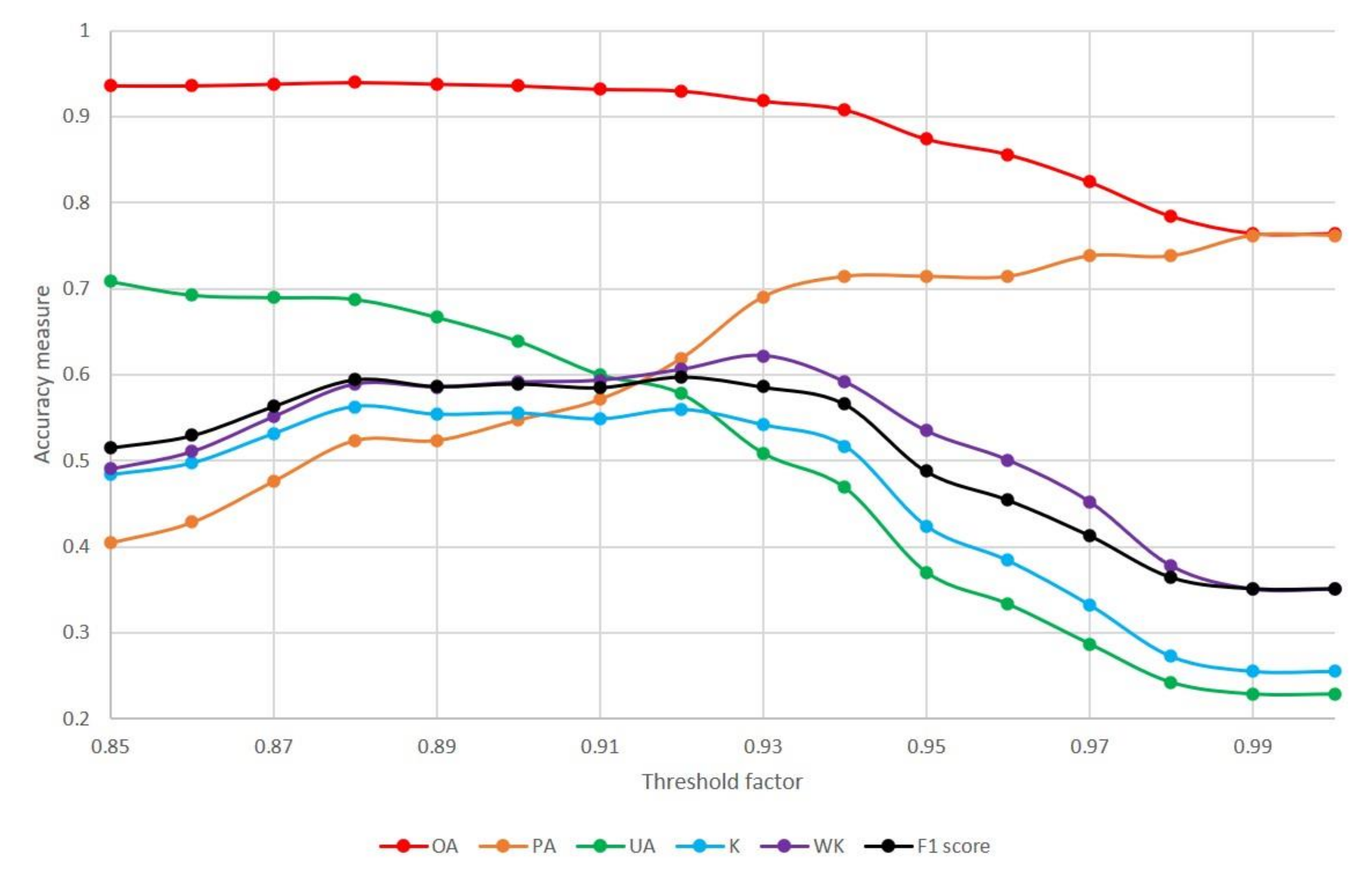
The method estimates for every pixel both a model for change and a model for no-change. The change model is accepted if the RMSE is smaller by a given threshold factor (h) than the no-change model. We tested all values of h between 0.85 and 1 in steps of 0.01. The selection of the appropriate threshold was based on the WK. The impact on the accuracy measures over the training period is shown in Figure 4. The threshold parameter (h) most strongly affects the UA and PA. F1 score is approximately equal for all thresholds between 0.88 and 0.93, with values decreasing outside this range. Increasing h means that more true changes are identified, increasing the PA, but also more no-change pixels are identified as having undergone change, decreasing the UA.

The weighted kappa coefficient (0.622) was used to determine the appropriate threshold value of 0.93. The corresponding overall accuracy is 91.8%, the user’s accuracy is 50.9% and the producer’s accuracy is 69.0%.

The trained model was then applied to the validation period 2006–2015 and assessed against an independent sample of ground truth data (Set B). The results give an assessment of where and when a transition in land cover occurred (Figure 5). The results indicate substantial contiguous areas of land cover change in the four areas where major urban development took place over the study period, these are suburban expansion in the Haydon Wick area and East Wichel, minor expansion of the South Marston industrial complex post initial construction, and construction of the new Blunsdon bypass (initial work began with archaeological excavations in 2006 [49]).

Changes outside of these known areas of urban growth are found within both the urban and rural environments. In the urban environment, identified changes are mainly in small patches (groups of contiguous pixels that change at the same time) or isolated pixels, whereas in the rural areas change occurs in predominantly large patches (Figure 5).

The accuracy of the validation change detection was assessed against 500 manually examined ground truth points (Set B) and the results are cross tabulated in a contingency table (

Table 3. Contingency table of model and ground truth data for the period of 2006–2015.

		Ground Truth			Total
		Change	No-Change
			Partial-Change	No-Change
Model	Change	24	6	23	53
	No-change	15	69	363	447
Total		39	75	386	500

). An overall accuracy of 91.2% for correctly identified change/no-change was found. The kappa index of agreement is 0.475 and weighted kappa is 0.486 (

Table 4. Accuracy measures and associated confidence intervals. The model shows three sets of statistics corresponding to three sets of analysis and three sets of accuracy assessment data (Sets A, B, and E). The training period are the values from the selected 0.93 threshold iteration. The validation model is directly comparable to the PCC as both use the same sample set (Set B). Time-of-change analysis was performed over the oversampled area of Haydon Wick for the increased time period of 2002–2015. Kappa values are presented with estimations of large sample variance using Delta method [46]. Note that for UA, OA, K, and F1 score, partial-change is counted as no-change. For WK, partial-change is in half agreement with change, and full agreement with no-change.

Metric	Model			PCC
	Training Period	Validation Period	Time-of-Change
OA (%)	91.8	91.2	86.0	72.6
K	0.542 ± 0.00835	0.475 ± 0.00678	0.720 ± 0.00616	0.181 ± 0.00177
K significant above 1.96	5.93	5.76	9.17	4.30
WK	0.622	0.486	0.762	0.198
PA of change (%)	69.0	61.5	87.2	69.2
PA of no-change (%)	97.6	94.0	94.7	73.8
UA of change (%)	50.9 ± 4.47	45.3 ± 4.45	83.7 ± 7.39	17.8 ± 3.42
UA of no-change (%)	97.1 ± 1.51	96.6 ± 1.61	88.2 ± 6.44	96.6 ± 16.3
Unbiased PA of change (%)	66.4 ± 13.6	61.7 ± 13.9	88.1 ± 8.31	71.4 ± 13.6
Unbiased OA (%)	92.3 ± 5.46	91.1 ± 4.72	85.9 ± 9.85	70.8 ± 4.31
F1 score of change	58.56	52.2	85.4	28.3

).

Using the method outlined in Congalton and Green [46], confidence intervals of overall, producer’s and user’s accuracy of change, and large sample variance of kappa were calculated. For Congalton and Green [46], confidence intervals require the use of unbiased producer’s and overall accuracy calculated from map marginal proportions not derived from the error matrix; however, this normalisation results in only a small variation of accuracy measure.

4.2. Post-Classification Change Detection

The PCC of the LCM 2007 and LCM 2015 identifies considerably more change than our method (Figure 6). The confusion matrix of the PCC (

Table 5. Confusion matrix of the PCC of LCM2007 and LCM 2015 with 500 ground truth pixels.

		Ground Truth			Total
		Change	No-Change
			Partial-Change	No-Change
PCC	Change	27	24	101	152
	No-change	12	51	285	348
Total		39	75	386	500

) results in an increased producer’s accuracy of change, yet user’s accuracy is greatly decreased compared to our analysis (Table 4). The great disparity between user’s and producer’s accuracy of change is reflected by a low F1 score (Table 4). This is also reflected in a poorer kappa and overall accuracy metrics due to an increased false positive rate.

By comparing the results of Set B between the model and the PCC it is revealed that the methods agree with change in a small proportion of pixels (

Table 6. Agreement between our model and PCC. Kappa statistic = 0.138. Note, these are not necessarily correctly identified, merely agreement between the two methods.

		PCC		Total	Agreement
		Change	No-Change
Model	Change	28	25	53	52.8%
	No-change	124	323	447	72.3%
Total		152	348	500
Agreement		18.4%	92.8%		70.2%

). The kappa statistic between the two methods is 0.138, indicating almost random agreement.

4.3. Type of Change

The type of change observed in the ground truth data for Set B, and the number of true positives and false negatives is shown in

Table 7. Manual classification of pixels identified as change. Columns show final land cover, rows show original land cover. First number indicates correctly identified change (true positives); second value (in brackets) gives the number of false negatives of the change class.

		Final Land Cover
		VE	VMS	SBU	BG	DBU
Starting Land Cover	VE	0 (0)	1 (1)	6 (1)	5 (0)	0 (0)
	VMS	0 (0)	1 (0)	1 (0)	2 (1)	0 (0)
	SBU	0 (0)	0 (1)	0 (2)	0 (1)	1 (0)
	BG	0 (0)	0 (0)	4 (5)	2 (1)	1 (1)
	DBU	0 (0)	0 (0)	0 (0)	0 (0)	0 (1)

. The most numerous changes were conversions of bare ground to sparsely built-up, vegetated to bare ground, and vegetated to sparsely built-up.

4.4. Time-of-Change

A further 100 pixels (Set E) were analysed in an area that saw substantial rural to urban change over the time-period of 2002–2015 to assess the temporal accuracy of our method. Of these, 47 pixels underwent land cover change, with the model correctly identifying 41. In addition, the model identified six pixels in the partial-change category as change; to assess what the model is detecting when it detects partial-change, these were included in the analysis (for a total of 47 pixels). Table 4 shows that the change detection rate in an area where there is considerably more change is vastly improved.

In the time-of-change accuracy assessment ground truth data, the period within which change occurred was between the time of the last image before the change and the first image after the change. For 42 (89.4%) pixels, the estimated time-of-change was within the period identified in the ground truth data (Figure 7). Of the five incorrectly dated pixels, the model determined change occurred more recently in four instances, with a maximum difference of five years. The middle value of the period of potential change is shown by the yellow line in Figure 7. The average time-period of potential change was 2.7 years with a standard deviation of 1.3 years. The model correctly dated all partial-change pixels that it detected as undergoing change.

4.5. Classification of Transition Types

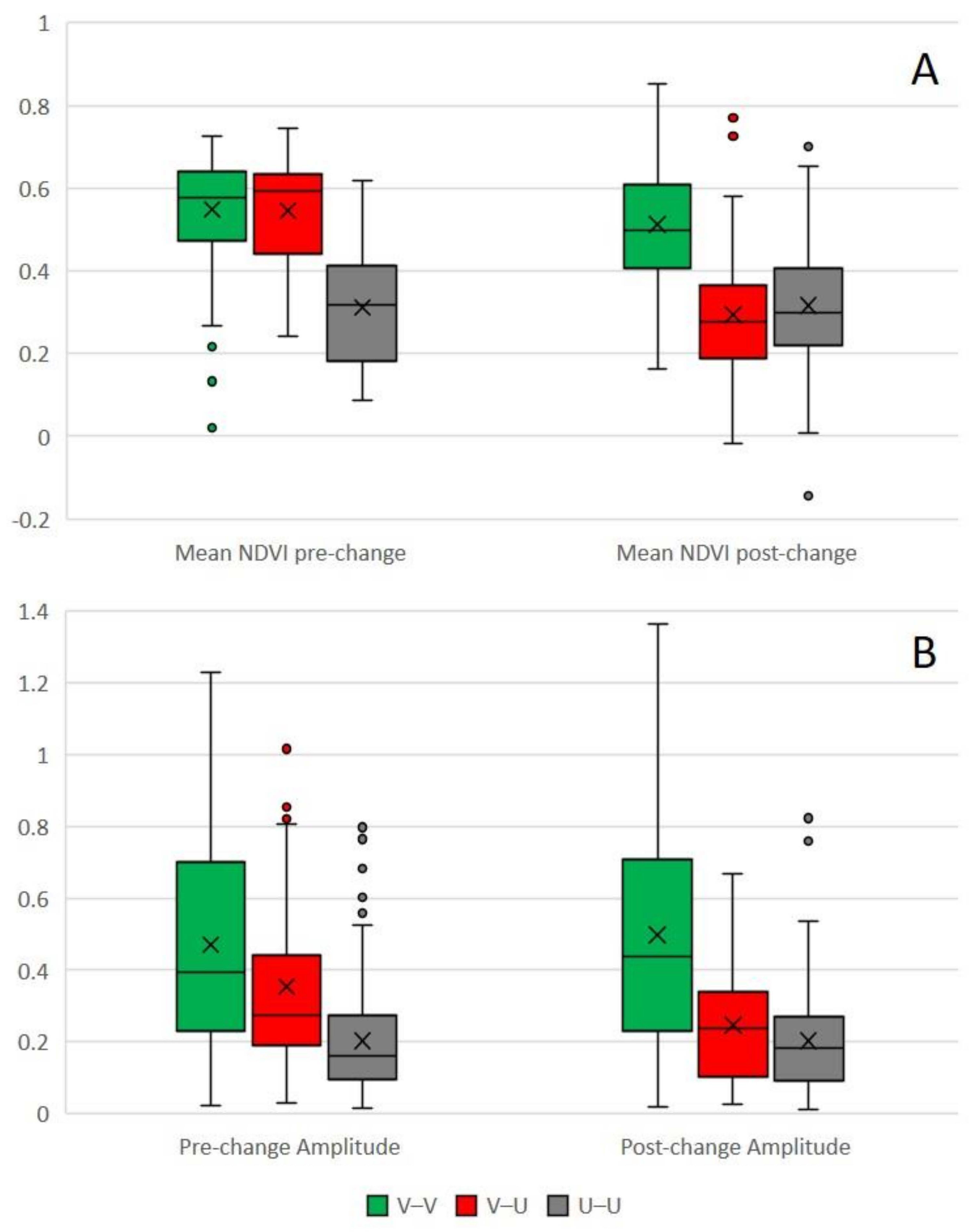
Before applying the random forest classification, we explored the distribution of the parameters over the three transition types to explore the separability based on this input data and classification scheme. The results show reasonable separation and are in line with the normal expectation that rural areas experience greater amplitudes and mean NDVI levels (Figure 8).

The final step of analysis was to classify the resulting change layer to understand rural to urban change, and this follows herein.

Ground truth data were gathered from 500 pixels and manually classified into vegetation to vegetation (222 pixels), vegetation to urban (107 pixels), and urban to urban (163 pixels) change. Five pixels undergoing urban to rural change, and three pixels covering mostly water, were excluded, leaving 492 pixels as training data. A random forest classifier was used to classify the validation map. The resultant layer of transitions (Figure 9) shows a clear urban gradient. The centre is dominated by urban to urban transitions, at the urban periphery rural to urban is the main transition type and in the rural areas, rural to rural transitions are most common. Applying the classification of growth patterns from Xu et al. [50], it appears that there is a degree of infill and leapfrogging, but the major pattern of growth is edge expansion.

For validation a further 300 randomly selected pixels from within the change class of the validation model were chosen Those which underwent urban to vegetation (two pixels) transitions and a single pixel which was dominated by water were removed, leaving 297 pixels for accuracy assessment.

The key statistics based of the confusion matrix (

Table 8. Confusion matrix of transition types for 297 pixels accurately classified as changed.

		Ground Truth			Total	UA
		V–V	V–U	U–U
Classification	V–V	133	17	5	155	85.8
	V–U	13	34	7	54	63.0
	U–U	4	4	80	88	90.9
Total		150	55	92	297
PA		88.7	61.2	87.0		83.2

) have an overall accuracy of 83.2% and a kappa statistic of 0.724. The lowest accuracies (both PA and UA) were observed in the V–U class.

4.6. Number of Clouds per-Pixel

The number of observations per-pixel ranged between 697 and 731, as not all images covered the entire study area. Per-pixel minimum and maximum cloud-free observations were: 72 (a highly mixed SBU pixel) and 343 (a pure VE pixel), respectively. These two pixels were investigated individually and were both correctly identified as undergoing no-change.

The cloud-free coverage for all pixels in Set B was tabulated by both model and ground truth classification (

Table 9. The average percentage of cloud-free pixels in Set B by change classification.

		Ground Truth
		Change	No-Change
			Partial-Change	No-Change
Model	Change	41.0	41.8	43.2
	No-change	41.8	42.0	42.2

). For pixels within this set, the minimum cloud-free coverage for a pixel was 158 (21.9%), and the maximum was 332 (45.8%). There is no obvious correlation between cloud-free coverage and change detection (Table 9).

Out of the 500 pixels of Set B, the 50 pixels with the highest number of cloud-free pixels, and the lowest 50 pixels were inspected to determine any correlation to land cover class. Of the lowest 50 pixels, only 10 involved rural classes (either change to for from V, or stable V); conversely, of the highest 50 pixels, 35 involve the V class. DBU is absent from the top 50 pixels, and VE is absent from the lowest 50 pixels.

5. Discussion

5.1. Detection, PCC, and Type, and Timing of Change

The manually classified class of partial-change is of particular interest. This class mostly coincides with no-change in the automated procedure, but holds 20.7% of the pixels misclassified as change, even though it only contains 16.3% of all no-change pixels (Table 3).

Nominally, a UA of 45.3% may be considered low; however, the model comfortably outperforms the common practice of PCC (UA = 17.3%). The PCC method used information from additional Landsat bands and ancillary data not used in this study. As a proof-of-concept, this demonstrates the viability of our method. Future studies may expand our method to incorporate other available information to improve accuracy and apply the method to a wider scale.

The relatively large confidence intervals on the PA of each model iteration may be attributed to the considerable proportional difference between the area (or total number of pixels) of change vs. no-change (including partial-change) (Table 4). In the threshold and validation time periods, the ratio of change vs. no-change area is approximately 1:11. Similarly, due to the small area of change relative to no-change, the UA will be negatively impacted by a moderate proportion of error in the non-changing land (false positives). In the time-of-change analysis, however, the proportion was approximately 50:50. This run yields the lowest confidence interval on the PA and highest UA of change, suggesting a stratified random sample should be recommended for future change detection research and would likely increase the UA of this study. The drastically improved UA (relative to the training and validation runs) of the time-of-change analysis, however, may be an artefact: as most observed changes were from a rural to an urban land cover, these changes undergo large drops in NDVI (Figure 8A), which our model is optimised to detect. In the time-of-change analysis, a slight majority (51.1%) of correctly identified pixels are above the middle of the date range (Figure 7), suggesting a robust method of dating change.

The disparity between the PA and UA of the PCC is clearly demonstrated via the lowest F1 score of any change detection (Table 4). The greatly increased PA comes at the expense of a reduced UA, which is reflected in other statistics, particularly the K. This is in line with the theoretical expectation that PCC overestimates changes as classification errors in either layer are registered as change [6] and is a known issue with the method. The PCC detects the most change, reflected in Table 6 and Figure 6. In principle, however, PCC analysis should find fewer changed pixels, as it excludes changes within a land cover class. Furthermore, the LCM uses a minimum mappable unit and, hence, fine-grained changes are less likely to be registered.

Table 7 shows that the most commonly detected and occurring changes were BG–SBU, VE–BG, and VE–SBU, clearly demonstrating the large proportion of urban growth occurring in Swindon during the study period. These changes reflect the suburban expansion via the conversion of rural fields to either worksites or constructed housing, or the completion of worksites to housing. The high accuracy of detection of conversions of VE to either BG or SBU likely reflects the dramatic change in NDVI values which would accompany this type of change (Figure 8A). Similarly, the poor detection of BG to SBU may be due to the similarity of NDVI values between these classes.

The model most frequently confuses vegetation to urban with vegetation to vegetation; this may be due to the relative greenness of some urban areas, as indicated by Figure 8, which shows some overlap between these two classes. Figure 8 suggests that the value of the mean NDVI trend before and after change may be a better predictor of transition type than amplitude due to the lack of overlap of the boxes of the plots. To improve change detection and classification accuracy, the inclusion of other vegetation indices is an avenue for further research. This can be achieved by the substitution of NDVI for other indices into Equations (1) and (2).

5.2. Impact of Landsat Archive

This methodology uses the entire Landsat 5, 7, and 8 archive up to 2018 to detect change for the period of 2006–2015. This period of analysis was chosen to facilitate comparison with the LCM products and coincide with the availability of the high-resolution imagery used as ground truth data. This model requires at least one year prior to and after the period of change for this to be detected. Zhu and Woodcock [14] note that this initialisation period can impact the outcome of the change detection algorithm. This may manifest in two ways: firstly, the method is limited to detecting one instance of change per pixel; therefore, change occurring outside of the period of change detection can mask change in the period of analysis. Multiple changes in the same location are unlikely; however, they are entirely possible. Urban growth is typically unidirectional; therefore, multiple changes are unlikely. The purpose of our study was to detect urban growth; therefore, the detection of a single change is a reasonable assumption; however, this may not be universally true. Only a single pixel in all those analysed underwent two land cover changes in the period between 2002 and 2015 (excluding transitionary land cover types such as worksites); however, partial-change was often associated with longer-term incremental changes totalling <50% of the pixel (such as extensions and garden development over several years).

Secondly, the length of lead-in time may yield a poorly fitting model. The model assumes that the best fitting sinusoidal function pair will have resulted from a land cover change. This may not be the case, as the considerable lead-in period allows for large fluctuations in the bounded NDVI value (as NDVI cannot vary outside of −1–1), which may not be accurately quantified by the linear component of a single sinusoidal function. Any non-zero NDVI trend must at some point change, as NDVI cannot increase or decrease ad infinitum. Therefore, the lead-in period may swamp the analysis and cause an incorrect estimation of $\tau$, as the model may find this yields a lower RMSE than the correct time-of-change, leading to an incorrect change detection. Finally, the considerable mismatch between the lead-in and -out length may have impacts on the change detection accuracies that were not explored. The choice of these dates was constrained by the availability of ground truth data, and it is postulated that change detection would be most accurate when these periods were approximately equal. The length of the lead-in and -out period, and the impact on change detection were not investigated and is a subject for future research.

5.3. Computation Time

Computationally, the most time-consuming step was the linear regression, estimation parameters of Equation (2). Note that this step requires multiple linear regressions for each pixel. This was performed on GEE cloud servers and took approximately 24 h. The implementation of Equation (3) and the random forest classification took less than 10 min. As a pixel-based algorithm, the computation time is expected to vary proportionally with the number of pixels.

5.4. Impact of Changing Spatial Resolution

The 30 m resolution of Landsat is well suited to the detection of housing unit construction but fails to adequately capture finer resolution changes, such as small increases in paved surface in gardens. Increasing the spatial resolution of the sensor (such as by using Sentinel 2) should not impact the accuracy of change detection in areas where the change is larger than the Landsat pixel size, but will aid the detection of smaller changes, that would be classified as partial-change at the Landsat resolution but complete change at the Sentinel 2 resolution.

Theoretically, this method requires only a single year of time series data before and after the change detection period. However, it is expected to be more accurate and advantageous than conventional pair date comparisons for longer periods, such as those of the Landsat archive. However, the ideal time series length is subject to further research.

5.5. Impact of the Number of Clouds on Change Detection Accuracy

The percentage of cloud-free pixels appears to be independent of classification accuracy (Table 9). We therefore find that in the current study, sufficient cloud-free images were available to not impede or bias the detection of change using this method. No testing was undertaken to relate the accuracy of the method to the number and temporal distribution of cloud-free observations. This can be addressed in the future by randomly deleting observations and applying the method.

6. Conclusions

This study investigated the use of structural break detection in harmonic analysis to detect and classify land cover change in the context of urban growth. An advantage of the method is that it is based on the detection of a change of trend that is manifested over a period. Hence, it is less sensitive to noisy and missing data, for instance due to cloud cover and shadows, as is prevalent in the case study area. To detect change in any year, the model requires a lead-in and -out period, therefore limiting usability in creating current maps. Further work may assess the feasibility of smaller time units, such as six months. The case study considered changes occurring between 2006 and 2015 but used the full archive from 1984 to 2018.

The method clearly outperforms PCC, even for a land cover product that is in many senses superior to our approach; unlike the LCMs, we only considered temporal variation in NDVI and did not make use of ancillary data. We therefore consider the application a successful proof of concept. In particular, the proposed method does not suffer from the considerable bias toward detecting change of PCC and provides an accurate estimation of the time-of-change. Notwithstanding, there is substantial scope for improvement: the detection of changed pixels has a user’s accuracy of 45.3 ± 4.45%, and a classification user’s accuracy of rural to urban of 63.0%.

Further refinements to improve the accuracy, aside from incorporating data from other sources, are possible. One avenue is to make fuller use of the spectral information in the Landsat archives, beyond NDVI. Other options are to expand the model to allow for multiple change events per pixel over time, particularly to detect transitional land cover classes, and to integrate changes in the fit between model and data in the identification of structural breaks. Finally, the method may be applied to other image collections with the capability of calculating NDVI such as Sentinel 2.