
DV-LOAM: Direct Visual LiDAR Odometry and Mapping


State Key Laboratory for Information Engineering in Surveying, Mapping and Remote Sensing, Wuhan University, 129 Luoyu Road, Wuhan 430079, China
*
Author to whom correspondence should be addressed.
Remote Sens. 2021, 13(16), 3340; https://0-doi-org.brum.beds.ac.uk/10.3390/rs13163340
Submission received: 4 July 2021
/
Revised: 16 August 2021
/
Accepted: 18 August 2021
/
Published: 23 August 2021
Abstract
:Self-driving cars have experienced rapid development in the past few years, and Simultaneous Localization and Mapping (SLAM) is considered to be their basic capabilities. In this article, we propose a direct vision LiDAR fusion SLAM framework that consists of three modules. Firstly, a two-staged direct visual odometry module, which consists of a frame-to-frame tracking step, and an improved sliding window based thinning step, is proposed to estimate the accurate pose of the camera while maintaining efficiency. Secondly, every time a keyframe is generated, a dynamic objects considered LiDAR mapping module is utilized to refine the pose of the keyframe to obtain higher positioning accuracy and better robustness. Finally, a Parallel Global and Local Search Loop Closure Detection (PGLS-LCD) module that combines visual Bag of Words (BoW) and LiDAR-Iris feature is applied for place recognition to correct the accumulated drift and maintain a globally consistent map. We conducted a large number of experiments on the public dataset and our mobile robot dataset to verify the effectiveness of each module in our framework. Experimental results show that the proposed algorithm achieves more accurate pose estimation than the state-of-the-art methods.

1. Introduction
The latest activity in the field of self-driving car navigation is considered to be the next revolutionary technology that will change people’s lives in many ways [1]. It triggered a series of reactions that aroused the automotive industry, and SLAM plays a key role in autonomous vehicles, especially in solving positioning problems in unfamiliar environments.Traditionally, the localization of autonomous vehicles rely on Global Navigation Satellite System, Inertial Navigation System (GNSS/INS) [2,3]. Yet, GNSS position information is prone to jump due to signal blocking, multipath effects, and magnetic noise [4,5], and INS may experience cumulative errors, especially in GNSS challenging environments, such as urban canyons, boulevards, and indoor environments. Therefore, studying the use of SLAM technology to solve the positioning problem in the GNSS-denied environment is of great significance to the realization of autonomous driving. In particular, the fusion method of camera and LiDAR is receiving more and more attention from scholars.
In recent years, great progress has been made in the field of visual SLAM using monocular cameras, including direct methods and feature-based indirect methods. The classical visual feature-based methods have matured, resulting in a stable visual SLAM method. Among them, the most popular are PTAM [6,7], ORB-SLAM [8,9]. However, the disadvantage of these feature-based methods is that it is difficult to finding the corresponding feature association when the environment is a simple repetitive pattern or a featureless condition. In Contrast to feature-based methods, direct methods have the potential to utilize complete image information, such as LSD-SLAM [10], DSO [11], SVO [12,13]. Since they only used a certain number of patches, or areas of image gradient magnitude above a threshold, to reduce computation complexity, so as to ensure that the direct method runs in real-time on the CPU and shows remarkable motion estimation performance despite not using the correspondence of visual features. However, monocular images are not sufficient to estimate the ego-motion, because movement along the optical axis of camera can only cause little motion of visual features, so the estimation problem may be degraded.
LiDAR-based SLAM systems have gained popularity over vision-based systems due to their robustness to changes in the environment and resistance to light illumination. Many of them are based on the Iterative Closest Point (ICP) method [14] or its variants [15,16]. At present, many Lidar SLAM methods [17,18,19,20,21,22,23,24] have been proposed, and all of them have achieved impressive results. Among them, the more representative one is LOAM [17,18], which is considered state-of-the-art in 6-DOF LiDAR SLAM. Afterward, Qin and Cao [25] simplified the feature extraction process and improved the efficiency of LOAM scan-to-map matching. However, pure LiDAR based systems have their shortcomings. Due to the limited number of laser beams in laser scanners, in the environment of repeated structures such as tunnels or corridors, the distance measurement in the vertical direction is quite sparse, they are prone to failure [26].
Since images provide rich visual texture information, and LiDAR has sparse but precise distance measurement and 360-degree field of view, the combination of vision sensors and lidar sensors may complement each other in motion estimation tasks. Similar work in visual lidar odometry can be found in references [27,28,29,30,31,32,33,34,35,36]. For example, the work of Shin et al. [30,31], namely DVL-SLAM, attempted to solve the visual laser SLAM problem within the DSO framework. They used projected laser points as feature points instead of using the salient gradient points extracted from the images. With the depth values of the feature points known and fixed, they performed the same multi-frame photometric optimization as DSO to estimate the poses of the keyframes. Since there is no need to extract and match features, and benefit from the precise distance measurements of the laser, it shows robust, efficient and accurate SLAM results even with extremely sparse depth measurements in a large-scale environment. However, DVL-SLAM [30,31] only used the laser points in the camera’s field of view, and most of the range measurements will be discarded because laser sensors like Velodyne LiDAR can provide 360-degree scanning. This setting makes the system less accurate and vulnerable to untextured scenes. For V-LOAM [32], it combined the visual odometry method DEMO [28,29], and the lidar odometry method LOAM [17,18]. The visual odometry handles rapid motion, while the lidar odometry guarantees low drift and robustness under poor lighting conditions, so it can handle aggressive motion including translation and rotation, as well as the lack of optical texture in complete whiteout or blackout imagery. Since odometry integrates small incremental motions over time, drift is bound to occur during long traversals. Therefore V-LOAM is not suitable for large-scale environments.
To alleviate this issue, loop closure is applied as a trigger to invoke pose-graph optimization by recognizing the revisited sites using either visual or LiDAR methods. Visual methods involve using Bag-of-Words (BoW) [37,38,39] to recognize the place and Perspective-n-Point (PnP) algorithm to estimate the posture correction. In LiDAR methods, the places are recognized using segment-based algorithms like SegMatch [40,41], or global descriptors based methods [42,43,44], and of course deep learning based methods [45,46], and pose correction is estimated using ICP algorithm. However, a revisited place usually varies from light illumination, weather, or viewing angle, which is difficult to be solved in vision-based place recognition. Although LiDAR is less affected by such environmental change. It lacks the fast and versatility of the BoW based methods, so it cannot perform global search. A local radius search based strategy is often needed to narrow the scope of the search to improve the efficiency of loop closure detection. However, this strategy may result in a reduction of recall rates when the accumulated drift larger than the search radius.
In this article, we introduce a novel Direct Visual LiDAR Odometry and Mapping (DV-LOAM) approach that combines the sparse depth measurement of LiDAR with a monocular camera. The system consists of three main parts as follows: Firstly, in the visual odometry part, we first use the depth-enhanced frame-to-frame direct visual odometry with a constant velocity motion model to estimate the initial motion of adjacent frames. As it directly uses the projected laser points as feature points instead of using the salient feature points extracted from the images, the efficiency is very impressive. Then, an optimization based on a sliding window is applied to refine the motion, which not only ensures real-time performance but also maintains the local accuracy of motion estimation. Secondly, in the LiDAR mapping part, each time a keyframe is generated, we apply a scan-to-map based LiDAR mapping process, which uses geometric features, such as lines and planes, to refine motion estimation and eliminate point cloud distortion caused by visual odometry drift. Finally, in the loop closure detection part, a Parallel Global and Local Search (PGLS) loop closure detection (LCD) algorithm is proposed to eliminate drift errors and obtain a globally consistent map. It first uses Bag of-Words (BoW) and LiDAR-Iris [44] technology in parallel to find loop closure candidates, then calculates a rough estimate of the pose correction using Truncated least squares Estimation And SEmidefinite Relaxation (TEASER) [47] algorithm, and finally refines the rough estimate using V-GICP [48]. In summary, the main contributions of this research are as follows:
- We proposed DV-LOAM, which is the first framework that combines a depth-enhanced direct visual odometry module and the LiDAR mapping module into location and mapping. It takes advantage of the efficiency of the direct VO module and the accuracy of LiDAR scan-to-map matching method, thereby further improving the performance compared to existing technologies.
- In the front end, we proposed a two-stage direct tracking strategy to ensure real-time performance while maintaining the local accuracy of motion estimation. Firstly, the direct frame-to-frame visual odometry is used to estimate the pose of camera, which is more efficient than ICP-based odometry. Secondly, a thinning module based on a sliding window is used to reduce accumulated drift. Since there is no need to extract and match features, this method is quite fast and can work even in low-texture environments.
- In the back end, a PGLS-LCD module was presented, by fusing the BoW and LiDAR-Iris techniques, our approach can not only greatly compensate for the insufficiency of vision-based LCD capabilities, especially in the case of reverse visit, but also alleviate the problem of not being able to find the correct loop closure when the accumulated drift exceeds the search radius of LiDAR-methods. In addition, using TEASER’s estimate as an initial guess, and applying V-GICP to refine the transform of pose correction between loop pairs, more robust and accurate results can be obtained even in the case of large drift.
- Extensive experiments have been conducted to test and verify the effectiveness of the system in detail from both quantitative evaluation and visualization clues, and analyze the accuracy improvement brought by each module at different positions of the baseline.
The rest of this paper is organized as follows. In Section 2, we gives a brief review of the related works. Section 3 introduces the proposed DV-LOAM architecture. The details of direct visual odometry, LiDAR mapping, and loop closing are presented in Section 4. Section 5 discusses the accuracy evaluation of the proposed DV-LOAM and the comparison with the state-of-the-art methods. The discussion and future work are presented in Section 6. Finally, the conclusions of this paper are presented in Section 7.
2. Related Works
Because the focus of this article is to study the fusion method of vision and LiDAR, only methods of vision LiDAR fusion are introduced here. The combination of visual sensors and lidar sensors as a visual LiDAR odometry realizes the advantages of the two sensors, so it has been more and more researched, which is of great help to modern SLAM applications. The common work of visual LiDAR odometry can be divided into three groups: visual odometry based approaches, point cloud registration based approaches, and tightly coupled fusion methods.
2.1. Visual Odometry Based Methods
The visual odometry based method attempts to apply a visual odometry pipeline with known pixel depth information from laser scanning. In LIMO [27], LiDAR measurement is used for depth extraction. After projecting the point cloud on the frame, motion estimation and mapping are performed using a visual keyframe based bundle adjustment. The work in DVL-SLAM [30,31] proposed a direct visual-SLAM using a sparse depth point cloud from LiDAR. They use the projected laser points as feature points instead of using the salient gradient points extracted from the images. With the depth values of the feature points known and fixed, they perform a multi frame photometric optimization the same as the DSO to estimate the poses of the keyframes. The work of Zhang et al. [28,29], named depth enhanced monocular odometry (DEMO) is similar. The method associated the visual feature with depth measurement and uses it to estimate the camera motion. Recent of the development of the low cost solid-state LiDAR, there are also emerging in large numbers visual LiDAR fusion approaches using the Field of View (FoV) LiDAR, such as RLIVE [49], and CamVox [50]. Compared with the traditional mechanical LiDAR, although the FoV is smaller, the solid-state LiDAR is relatively cheap and has a higher point cloud density. CamVox [50] was built upon the framework of ORB_SLAM2, and it used Livox as the depth sensor to implement a new “RGBD” SLAM method. Since the accuracy and range of the lidar point cloud is superior compared to other depth cameras, CamVox showed higher efficiency and robustness even in an outdoor strong-sunlight scene. However, those methods did not taking the uncertainty of the fused information into consideration, such as the extrinsic calibration errors. In order to overcome these problems, Voges et al. [51] proposed to use interval analysis to model all errors, and introduced a bounded error model for the camera and LiDAR, so that the depth of feature points and the uncertainty of the depth can be estimated more accurately. However, a common problem of visual odometry based methods is that they do not consider the laser points that are outside the camera’s field of view, and most of the range measurements of LiDAR will be discarded. Such setting renders the system less accurate and vulnerable to texture-less scenes.
2.2. Point-Cloud-Registration Based Methods
Compared with the method based on visual odometry, the point-cloud-registration based approaches try to align the whole point cloud with the help of image information in various aspects. For example, the method in [33] and V-LOAM [32] simply uses the visual odometry result as an initial guess to the ICP process, making the ICP less likely to be trapped in local minima. Those algorithms follow the odometry framework without using SLAM techniques such as bundle adjustment and loop closure. However, the visual odometry used in these methods is a feature-based method, which means that features need to be extracted, but in a low-texture environments, it it difficult to extract enough features. Besides, using LiDAR for feature depth extraction is time-consuming and complicated, especially when the beam of LiDAR is limited, such as VLP-16. Besides, in order to deal with failures of ego-motion estimation, Reinke et al. [52] proposed an integrated visual-LiDAR odometry system that uses multiple odometry algorithms in parallel in frame-to-frame tracking stage. Then it selected the pose that best meets the constraints, including the dynamic and kinematic constraints of the vehicle, the Chamfer distance-based score calculated between the current LiDAR scan and a local point cloud map, thus exploiting the advantages of different existing ego-motion estimating algorithms. It showed great robustness and is resilient to failure cases. It also provided us a new idea to improve the robustness of the front-end odometry. In addition to calculating the pose transformation between adjacent frames, vision can also be used for loop closure detection, such as [53]. The BoW was used to detect loop closure candidates firstly. Then a LiDAR-based geometry certification strategy was conducted to validate the loop closure. Finally, a Pose Graph Optimization (PGO) was applied to obtain the global consistent trajectory. Although this method achieved good results, only relying on visual BoW to detect loop closure cannot solve the problem of reverse visits.
2.3. Tightly Coupled Fusion Methods
The tightly coupled fusion methods attempt to use vision and lidar measurements for more effective odometry estimation. Huang’s work in [35] proposed a lidar-monocular visual odometry approach using point and line features. Line features have conditional benefits, that is, they are less sensitive with problems such as noise [54], wide range of view angle [55], and motion blur [56], which are the main drawbacks for the point-only systems such as LIMO [27]. By leveraging more environmental structure information into pose estimation and a robust method for feature depth extraction, it greatly reduces the features’ 3D ambiguity, thereby improving the accuracy of pose estimation. Since LiDAR point cloud may contain occluded points that will reduce the estimation accuracy. The work in [36] solves this problem by proposing a direct SLAM method with an occlusion point detector and a coplanar point detector. Besides, to achieve high estimation accuracy, a two-stage registration strategy is adopted, which optimizes a joint objective that rewards both tight point cloud alignment as well as consistent image appearance. In order to maximally utilize the measurements from cameras and lidars, TVLO [34] independently operates two mapping pipelines to construct two different maps, namely the lidar voxel map and the visual map. The input lidar points are matched to a lidar voxel map to formulate lidar geometric residuals, and visual features are matched to the visual map to compose stereo projection residuals. By maintaining visual and lidar measurements separately, TVLO is not affected by the potential problems of assigning the depths of lidars to non-corresponding visual features and incorporates more geometric constraints than the existing methods [27,28,32] when to solve odometry residuals. However, each frame in TVLO requires the above-mentioned feature extraction and pose optimization, which is vary time-consuming.
Similar to the proposed method is DVL-SLAM [30,31]. Compared with DVL-SLAM, our method has made the following improvements. Firstly, a frame-to-frame tracking strategy is used to estimate the motion of adjacent frames. In comparison with the frame-to-keyframe approach, it shows better robustness in various complex environments, such as highway and residential areas. In addition, the sliding window optimization module refines the pose of each frame instead of the keyframe in DVL-SLAM to maintain a higher local accuracy. Secondly, beacuse DVL-SLAM only uses the LiDAR points in the camera’s field of view, the system is less accurate and vulnerable to scenes with less texture. In this paper, we use a LiDAR based scan-to-map matching method to reduce the drift accumulated by the VO module, which greatly improves the accuracy and robustness of positioning, in particular an urban environment with rich structural information. Finally, compared with the BoW based place recognition module adopted by DVL-SLAM, our PGLS-LCD method takes both advantages of BoW and LiDAR-Iris, thus acquiring better performance, especially in reverse visit events.
In addition, V-LOAM [32] also shows similarity to our method to some extent. However, there are also several obvious differences as follows. Firstly, we use direct-based visual odometry instead of a feature-based tracking method to estimate rough motion. Since we directly use the projected laser points as feature points instead of using features extracted from the image, and without fitting the depth of features using laser scan like V-LOAM, our method performs better robustness, efficiency, and accuracy in the VO module. Moreover, since most SLAM methods assume the world is static, moving objects in the real environment may reduce the accuracy of scan matching. In order to alleviate the influence of dynamic objects, the LiDAR mapping module of our method adopts two additional strategies. First of all, we use the feature extraction method described in LeGO-LOAM [19], which avoids features extracted from noisy areas such as vegetation and small clusters. The second is a two-stage LiDAR registration strategy used in [57]. We first perform pose optimization using a small number of iterations. Then, the optimization results are used to calculate residuals, and after removing the largest residuals, a complete posture optimization is finally performed to obtain a more accurate posture. Finally, the consistency of the trajectory in a large-scale environment of our method is maintained by incorporating our PGLS-LCD and pose graph optimization module.
3. System Overview
An overview of the proposed method is illustrated in Figure 1. The system consists of a front-end and a back-end module, similar to the general SLAM approaches. The input of the algorithm is time-synchronized sequential image data and sequential LiDAR scans (for example, by using hardware trigger), and their relative transformation on the robot is known. At the front end, there are two main parts, a Visual Odometry (VO) module and a LiDAR mapping module. Firstly, when a new frame, an image with an associated sparse depth, is coming, the direct frame-to-frame tracking module (Section 4.2) is applied to estimate initial motion at first. Once the tracking process is successfully executed, the sliding window optimization module (Section 4.3) will refine the initial pose to maintain local accuracy while ensuring real-time performance. Then, if the criterion for generating the keyframe is met, the pose is further refined through the LiDAR Scan-to-Map Optimization method (Section 4.4). The back-end includes a loop closure detection module and a pose graph optimization module. The proposed PGLS-LCD (Section 4.5) is used for place recognition. When a loop closure is detected, the global pose graph optimization (Section 4.6) will be conducted to maintain global consistency, and the local LiDAR map used by lidar scan-to-map optimization module will be updated simultaneously.
4. Methods
4.1. Notation
A frame contains a gray image and a sparse LiDAR point cloud . Note that the LiDAR point cloud is transformed into camera coordinate. Each point can be projected to image pixel coordinate using a projection function .
We use a transformation matrix to represent the pose of a frame in the world coordinate, where n represent frame index. Thus the relative pose transformation between and can be obtained as:
And it can be applied for coordinate transformation of points between the different coordinates, as shown below:
where and are points in each frame, and are a rotation matrix and translation vector, respectively. Lie algebra , and are angular and linear velocity vector, respectively.
4.2. Direct Frame-to-Frame Tracking
The direct frame-to-frame tracking module performs the tracking process for fast motion estimation without using visual features. Since the use of the entire LiDAR point will reduce the efficiency of frame-by-frame calculation, and the point in the low-texture area has a limited role in motion estimation. While maintaining the accuracy of motion estimation, in order to reduce the computational complexity, it is necessary to first down-sample the laser points effectively. Then a patch-based direct tracking method is being conducted to estimate motion between adjacent frames. Unlike indirect methods, the tracking occurs at a fast rate without requiring corner-like feature extraction and matching. In addition, using only LiDAR-associated points eliminates a triangulation phase to estimate the depth, this simplicity benefits various robotics systems with cameras and LiDAR. Similar to other direct approaches [11,12], image pyramids and constant motion model strategies are also used to speed up the tracking process. The details are shown as follows.
4.2.1. Salient Point Selection
Although the measurements of LiDAR are already sparse, the points we use to estimate motion are even less, thus improving computational efficiency. The detailed process of selecting salient points is described in [30,31]. It is worth mentioning that this similar strategy is widely used in various SLAM methods, including direct [11,12] and indirect methods [8,9]. Figure 2 shows an example of selected salient points.
4.2.2. Patch Pattern Selection
Compared with pixel-by-pixel tracking, the patch-based tracking method [11] guarantees sufficient performance and robustness, while requiring slightly fewer pixels. However, the computational complexity increases with the size of the patch. The patch pattern we used in this paper is shown in Figure 3a.
4.2.3. Frame-to-Frame Tracking
Unlike DVL-SLAM [30,31], in the tracking phase, we use a frame-to-frame tracking strategy instead of frame-to-keyframe tracking for the following reasons: Firstly, the overlapping field of view between adjacent frames is larger, which means that more constraints can be incorporated to solve odometry residuals. Secondly, the shorter the time interval, the smaller the change in environmental illumination, and the more consistent the assumption of luminosity consistency of the direct method is. Finally, the shorter the time interval, the smaller the robot movement changes, and the more it conforms to the constant velocity motion model.
As showed in Figure 3b, the salient point of the last frame is projected to the image of the current frame through a initial transformation obtained by the constant motion model. Then the photometric residual of the corresponding point can be defined as:
In addition, changes in exposure setting, or ambient light of environment may have a large impact on direct-based methods. To address this issue, we add the photometric parameters to the equation, namely a gain and a bias parameters, which can be represented as: . Both and are unknown parameters, and will be estimated during the optimization, the details can be found in [10]. Therefore, the new photometric residuals can be defined as:
Thus, the object function used to estimate motion between the adjacent frames can be defined as below:
where is the sparse pattern patch of the salient point , shown in Figure 3a and the weight function we use is described in [58], which is calculated in each iteration.
Here, the degree of freedom is set to 5, and the variance of residual is obtained in each iteration while performing the Gauss-Newton optimization. The impact of the t-distribution based weighting function can be found in [58]. It should be noted that, for more efficient calculations, an inverse compositional strategy is also adopted here. For more information about the strategy, please refer to [12]. Besides, we also use a coarse-to-fine strategy to avoid optimization from local minimums and to handle large displacements in the optimization as shown in [30]. In this paper, the number of layers of the image pyramid is set to , and the maximum number of iterations for each layer is .
4.3. Sliding Window Optimization
The sliding window maintains a fixed number of keyframes to achieve the constant processing time of the VO module, improve local accuracy, and reduce computational load. Compared with the sliding window optimization in DVL-SLAM [30,31], there are two main differences in this paper are as follows. On the one hand, the sliding window in our approach is used to refine the pose of each frame instead of the keyframe. On the other hand, the poses of the keyframes in the sliding window are fixed, and only the pose of the current frame will be refined during the optimization process. The specific processes are introduced in the following sections.
4.3.1. Window-Based Optimization
This section details the pose refinement through a sliding window-based optimization process. In the previous section, the tracking process estimates 6-DOF relative motion by frame-to-frame. Once the tracking process is successfully performed, the pose of the current frame will be further refined through the sliding window optimization process to reduce drift and improve local accuracy. Like the frame-to-frame tracking module, we also use the photometric error model. The main difference from the frame-to-frame tracking process is that the sliding window optimization is performed on the global map coordinates. And we use the patches of the multiple keyframes in the sliding window to refine the pose of current frame.
As we can see from the Figure 4, each keyframe in the sliding window has its own associated image , salient LiDAR points , and pose . A point in the first keyframe of is projected into the image of current frame through the coordinate transform matrix . Given that the poses of the keyframes are defined in the map coordinate, we can obtain the initial transform through the equation:
where is the pose of current frame obtained from the frame-to-frame tracking, and represents the pose of the first keyframe in . Thus the residual of the point between the current frame and the first keyframe is defined as follows:
Then, for each salient LiDAR point in each keyframe in the sliding window, the photometric residual can be acquired by the above Equation (9).
Eventually, we can update the pose of the current frame using the object function (10) shown as below:
where is the number of keyframes in the window, indicates the salient points of the keyframe shown in Figure 2b, and means the patch of the sparse pattern as shown in Figure 3a. The weight function uses t-distribution, as described in the previous section. The complete two-staged depth-enhanced direct visual odometry algorithm is summarized in Algorithm 1.
| Algorithm 1 Two-stage based Direct Visual-LiDAR odometry. |
|
4.3.2. Keyframe Generation and Sliding Window Management
The number of keyframes in the sliding windown is maintained with a fixed number . The sliding window maintains a fixed number of keyframes to achieve a constant processing time of the VO module. The criteria we use to generate keyframe and manage sliding window is overlap radio and time interval , which is same as DVL-SLAM, and more details can be found in [30,31].
4.4. LiDAR Mapping
Since the LiDAR sensor has the advantages of high measurement accuracy, strong anti-interference ability, and wide sensing range and viewing angle, thus each time a new keyframe is generated, the pose estimated by the visual odometry is further refined by the LiDAR mapping module. The LiDAR mapping module contains two major steps. One is a LiDAR feature extraction and undistortion step, and the other one is a scan-to-map registration step.
4.4.1. Feature Extraction
The feature extraction module is composed of three sub-processes shown in Figure 5. Firstly, a fast line-fitting based ground extraction method [59] is used to segment the original lidar point cloud to ground point cloud and non-ground point cloud. Then, the non-ground is segmented into point clusters by a range-image-based segmentation approach [60]. Finally, after removing those small clusters, the edge features and planar features are extracted from the rest clusters following the process described in LeGO-LOAM [19]. A visualization of the feature extraction processes is shown in Figure 6a–f. It should be noted that, unlike in LeGO-LOAM, our planar feature points do not contain ground points.
4.4.2. LiDAR Feature Undistortion
Since the laser point cloud is not acquired at the same time, some distortion will occur during the movement of the data acquisition platform. In order to reduce the influence of LiDAR distortion on motion estimation, we adopt a Lidar undistortion method based on linear interpolation. The details of linear interpolation can be found in [17,18], and the relative transfrom needed by linear interpolation is obtained by the VO module. Eventually, we can obtain the feature point clouds of current keyframe without distortion, they are ground features , edge features , and planar features , respectively.
4.4.3. Scan-to-Map Matching
So far, we have got the initial pose , and the LiDAR features of the current keyframe . Now, the LiDAR scan-to-map matching module matches the features in , , to a surrounding point cloud map respectively, to further refine the the pose, and then merge the features to local point cloud map using the refined pose. Note that in order to improve efficiency, the feature point cloud and local feature map have already been downsampled with a voxel-based filter implemented in PCL [61], and the resolution of edge features, planar features, and ground features are , , and , respectively. In addition, the KD-Tree [62] method is also used to accelerate the speed of feature association.
The scan-to-map registration consists of two types of residuals, they are residuals of point-to-line, and residuals of point-to-plane, which are shown in Figure 7b,c, respectively. And the details of the registration process used in this paper can be found in Loam_livox [57]. The only difference is that we treat the ground feature points as separate features in the optimization, but the residuals of ground feature points are the same as planar feature points.
4.5. Loop Closure Detection
Loop closure detection is an essential and challenging problem in SLAM to eliminate drifting error. More importantly, it can also prevent the same landmark from being registered multiple times, thereby creating a globally consistent map, which can be used for robot positioning later. This section will focus on the following parts: Firstly, we briefly introduce the existing vision and laser-based loop closure detection methods and their problems in Section 4.5.1. Then, in response to the existing problems, we introduce the ideas and overall process we adopt in Section 4.5.2. Finally, the specific process of our method will be introduced in the following sections from Section 4.5.3–Section 4.5.5.
4.5.1. The Existing Vision and LiDAR Based Loop Closure Detection Methods and Its Problems
Existing works on loop closure detection consist of vision based methods and LiDAR based methods. We evaluated the performance of the BoW and LiDAR-Iris approach on the KITTI dataset, and the results were shown in Figure 8. The ground truth of loop closures was generated according to protocal B strategy in [44]. In KITTI sequence 05, all closed loops occur in the same direction, while in KITTI 08, the vast majority of closed loops occur in the opposite direction. In the Bow affinity matrix, the larger the value in the image, the higher the similarity between the two frames, while in the LiDAR-Iris affinity matrix, the smaller of the value in the image, the higher the similarity between the two frames.
As shown in Figure 8, the BoW method reported high precision on sequence 05 with only loop closures in the same direction. However, when the sequence only contains loop closures in the opposite direction, such as the KITTI sequence 08, it could not detect any loop closures, while the LiDAR-Iris method achieved promising results in both same-direction and opposite-direction loop closure events. However, LiDAR-Iris still had some shortcomings. On the one hand, many negative match pairs also exhibited low matching values, which would greatly increase the burden of verification. On the other hand, in the experiments we evaluated in the KITTI sequence 05 and KITTI sequence 08, the average computation time for extracting binary features from LiDAR-Iris image and matching two binary feature maps was about 0.021s. Therefore, a radius search strategy needed to be applied to ensure efficiency in the SLAM system. However, when the accumulated drift was larger than the searching radius, this strategy may lead to missed detection.
4.5.2. Parallel Globala and Local Serach Loop Closure Detection Approach
The flowchart of proposed PGLS-LCD approach is shown in Figure 9. For each newly added keyframe, the features will be extracted firstly, including ORB features used for BoW and the global feature LiDAR-Iris. Then, the loop closure candidates will be extracted using BoW and LiDAR-Iris technologies parallelly. Once loop closure candidates are successfully extracted, a consistency verification process is used to check whether there is a true-positive loop closure. After that, the correct transform will be estimated using the TEASER [47] firstly, and then refined by V-GICP [48]. Finally, the accurate transformation is added as a constraint to the pose graph. And when the pose graph optimization is completed, the loop database and point cloud map will be updated according to the newest pose of keyframes. The specific process is introduced in the following chapters.
4.5.3. BoW Vector Extraction and LiDAR-Iris Descriptor Extraction
Each time a new keyframe is inserted in the back-end, the ORB features shown in Figure 10c and LiDAR-Iris feature shown in Figure 10b are first extracted. Then, the ORB features will be transformed into BoW vectors through a vocabulary generated offline. Besides, a binary feature map is extracted with four LoG-Gabor filters from the LiDAR-Iris image Simultaneously. Therefore, a keyframe can be represented with and .
4.5.4. Loop Candidates Extraction
To prevent false positives, we use a dynamic similarity threshold as criteria for allowing loop candidates, and the threshold is calculated using the current keyframe and its adjacent keyframes. It is worth mentioning that ORB-SLAM2 also uses this method to improve the performance of loop closure detection. The complete loop closure candidates extraction process is summarized in the Algorithm 2.
| Algorithm 2 Loop closure candidates extraction. |
|
4.5.5. Consistency Verification
Given a new query keyframe and a candidate keyframe . As discussed in previous section, the global descriptor LiDAR-Iris is a highly simplified representation of original point cloud. Hence it is inevitable to have some features ignored, which can lead to false positive. And similarly, if there are analogous or repeated scenes, false-positive will easily occur when using BoW based method. Therefore it is necessary to check the consistency before closing the loop. In this paper, we use the following two consistency verification:
- Temporal consistency check:In a SLAM system, it is observed that the occurrence of single loop closure often implies high similarity on the neighbour since the sensor feedback is continuous in time [63]. We can verify the loop closure by measuring the BoW temporal consistency and LiDAR-Iris temporal consistency :where is the number of frames included for temporal consistency verification, and represent the similarity of BoW and LiDAR Iris, and the specific calculation method can be found in [37,44] respectively. Note that if the difference of viewing angle between and is larger than 90 degrees, and become and accordingly. The loop candidate can be accepted by taking threshold on the final temporal consistency score.
- Geometry consistency check:The geometry consistency check procedure is shown in Figure 11 below. The Fast Point Feature Histogram (FPFH) [64] features are extracted from the local point cloud map constructed from the neighbors of query and candidate keyframe respectively, and then being matched to find feature correspondences. Afterwords, TEASER [47] is used to get an initial guess of the rigid transform matrix through the feature correspondences. Finally, starting from this initial estimate, V-GICP [48] is applied to find minimal distance error between the local point cloud maps generated from the query keyframe and the candidate keyframe . If the fitness score is lower than a threshold , then a loop closure is detected successfully, and the relative pose transform is added to the pose-graph as a loop constraint.Note that, when using ICP based approach, or a direct tracking method (such as in DVL-SLAM), an initial transform is required to calculate the relative pose transformation. However, the initial guess is often unknown in the loop closing module. Therefore, those methods are easy to fall into the local extremum. In this paper, we use TEASER to get an initial guess of the rigid transform matrix. TEASER is a global registration method, which is invariant to initial transform, thus making our approach more robust.
4.6. Pose Graph Optimization
When the relative pose transform is obtained between the query keyframe and candidate keyframe, we add it to the pose-graph as a loop constraint, and a global pose-graph optimization implemented with CeresSolver will be conducted to reduce drift. Note that the local point cloud map used by LiDAR mapping will be updated after pose-graph optimization. Besides, each time we complete a pose-graph optimization, the loop closure detection process will pause for a period of time to ensure efficiency.
5. Results
To evaluate the performance of our method, the KITTI dataset [65], NuScenes dataset [66] and field test experiments are carried out where the monocular camera and the LiDAR sensor can be used simultaneously, respectively. The proposed method is implemented with C++ under Ubuntu 16.04 and robot operating system (ROS) [67]. A consumer-level laptop with an Intel Core i7-7700 and 32 GB RAM is used for all experiments. The main parameters applied for the algorithm are introduced in Table 1. Note that the other parameters used in our system is same as references. The experiments of our approach are organized as follows. Section 5.1 first introduces the results on the KITTI dataset to verify the performance of our method in large scenarios. In Section 5.2, we evaluated our method on the NuScenes dataset to verify the robustness in various scenarios, such as rain or dark night environments. Section 5.3 shows that our method performs better in the real environment compared to the state-of-art LiDAR-based methods. In Section 5.4, we analyze in detail the role of each module in our algorithm, including the depth-enhanced direct frame-to-frame odometry, the sliding-window-based optimization module, and the dynamic object-aware LiDAR scan-to-map registration module. Section 5.5 shows the loop closure detection results of our approach. Finally, Section 5.6 introduces the time efficiency of each module.
5.1. Validation on the KITTI Odometry Dataset
We use the KITTI sequences 00-10 with ground truth trajectories to evaluate the performance of our approach. And the results of these sequences without loop closure (-) and with loop closure (*) are reported in Table 2 for comparison, including the state-of-the-art LiDAR-based frameworks: LOAM, A-LOAM, LeGO-LOAM, and the state-of-art visual-LiDAR fusion based methods, such as DEMO, LIMO, DVL-SLAM, and the work of Huang et al. [35]. It should be pointed out that the results of LOAM, DEMO, LIMO, DVL-SLAM and Huang et al. [35] are directly quoted from articles, and no rotation error data is provided.
The evaluation result of our method in the KITTI odometry training dataset is using the KITTI evaluation odometry tool (www.cvlibs.net/datasets/kitti/evalodometry.php, accessed on 2 July 2021). The relevant trajectory error length is the mean value of 100–800 m length: relative translational error in %/relative rotational error in degrees per 100 m. Note that all trajectory are transformed into camera 0 coordinate and the comparison with the ground truth is shown in Figure 12.
5.1.1. Accuracy Comparison with Existing Methods without Loop Closure
To verify the performance of odometry, the proposed algorithm was applied on the KITTI odometry benchmark dataset by excluding loop-closure. As we can see from the Table 2, we have obtained an average relative translation error of 0.80% and a relative rotation error of 0.0038 deg/m in the entire KITTI odometry training dataset, which is outperforming than those state-of-art visual LiDAR odometry fusion approaches, such as DEMO, LIMO, the work of Huang et al. [35], and DVL-SLAM. DEMO and LIMO are visual odometry based fusion approach, the depths of features in DEMO are acquired simply by using triangulation meshes, while in LIMO, a more complicated feature depth extraction strategy of fitting local planes is applied. Besides, keyframe selection and landmark selection are employed in the procedure of Bundle Adjustment. Therefore, LIMO obtains better accuracy than DEMO. Compared with LIMO, although the rotation error of our approach was larger, we achieved a higher position accuracy, the relative translation error dropped from 0.93% to 0.80%. The reasons are as follows. On the one hand, the extraction accuracy of visual features can reach sub-pixel level, feature matching is relatively stable, and is not easily affected by factors such as illumination. Therefore, feature-based methods generally have more accurate rotation accuracy than direct-based methods. On the other hand, compared with monocular cameras, LiDAR sensors have high-precision ranging measurements, resulting in higher translation accuracy, especially in urban areas with rich structural information, such as sequence 00, 05, 06, and 07 shown in Table 2. Besides, semantic segmentation is required in LIMO to distinguish dynamic objects, such as cars and people in the environment, thus improving the robustness, accuracy, and avoiding the influence of moving objects. However, semantic information requires GPU computational resources and is usually time-consuming. Huang et al. [35] improved LIMO by leveraging points and lines for tracking and local mapping, and achieved almost the same translation accuracy compared with LIMO without using semantic information. Compared with Huang’s work [35], although our average rotation error was slightly higher, our translation error was significantly reduced from 0.94% to 0.80%. Our approach was developed from DVL-SLAM, and we achieved more accurate results by fusing the proposed two-staged direct VO module and a LiDAR mapping module, especially for the relative translation accuracy, which was improved considerably, and the translation error dropped from 0.98% to 0.80%.
Besides, compared with those LiDAR based methods, our approach also showed better performance than LOAM (translation error 0.84% in the paper), A-LOAM (translation error 1.49%, rotation error 0.0053 deg/m), and LeGO-LOAM. In addition, LeGO-LOAM failed in sequence 01, which is a highway scene where the vehicle is driving at high speed most of the time. The reason is that the scan matching module cannot extract sufficient features(edge features, and planar features except for ground points) for tracking.
Furthermore, we presented the rotation and translation error analysis according to path length and vehicle speed on the whole KITTI training dataset without using loop closing, and the comparison curves between DEMO, DVL-SLAM, LIMO, A-LOAM, the work of Huang [35], and ours were shown in Figure 13. As the speed increases, the accuracy of our method decreased slowly and then gradually increased, especially at higher speeds, the accuracy decreased very rapidly as shown in Figure 13a,b. This is the reason why our method performs relatively poorly on sequence 01, which is a highway environment with many dynamic cars, and the experiment platform moves very fast. The Figure 13c,d show the error according to the length of the vehicle’s moving path. As the cumulative path length increases, the relative translation error is decreases steadily as shown in Figure 13c, and the relative rotational error is also reduced as shown in Figure 13d.
The position and orientation of the proposed method changes on the KITTI odometry sequence 00 are shown in Figure 14. Our approach has significantly reduced the localization error of translation and orientation. Especially for the 2D pose components (x, z, yaw), which are approachable to the precision of ground truth. It should be noted that the position and orientation error of DV-LOAM mainly comes from the convergence accuracy of altitude, roll, and pitch, which have little impact on the navigation mission on flat terrain.
5.1.2. Accuracy Analysis and Global Maps Displaying with Loop Closure
Loop closure detection can help to correct the drift and maintain a global consistent map. In addition, these maps can be used for vehicle localization in GPS denied environments. As we can seen from Table 2, the average translation error and rotation error of our approach are 0.78% and 0.38 respectively. The globally consistent maps are built with keyframes, and more details can be seen from the LiDAR feature maps, as shown in Figure 15 bellow. It should be noted that to ameliorate the display effect, the ground LiDAR features are not shown in Figure 15.
5.2. Evaluation on NuScenes Dataset
We also evaluate our approach on the nuScenes dataset, which is a public large-scale dataset with many dynamic objects in the scene, such as cars and people. The results shown in Table 3 are obtained using nuScenes full dataset (v1.0) part 1. There are a total of 85 scenes, and none of those scenes have a loop closure. Besides, the trajectory length of each scene is shorter than 200 m, thus we calculate the average rotation and translation errors by dividing the trajectory into segments using 5 m, 10 m, 50 m, 100 m, 150 m, 200 m as did in [35]. In summary, we achieved an average translation error of 3.03% and an average rotation error of 0.0399 . The maps shown in Figure 16 are constructed using the poses estimated by our approach.
5.3. Evaluation on Our Campus Dataset
To verify our algorithm’s accuracy in the real world, an on-site experiment using our mobile robot camera-LiDAR platform shown in Figure 17b was conducted. The BUNKER (https://www.agilex.ai/product/1?lang=en-us, accessed on 2 July 2021) mobile robot platform was mainly equipped with an Nvidia Jetson Xavier, a ZED2 stereo camera, and a VLP-16 3D LiDAR. The robot accumulated almost 4500 frames after 7.5 min of driving at an average speed of 1.0 m/s. It’s worth mentioning that the data was recorded around two o’clock in the afternoon at Wuhan University, so there were many pedestrians and vehicles on the road.
5.3.1. Camera LiDAR Extrinsic Calibration
Ours previous work CoMask [68] was used to calibrate the extrinsic parameters between a monocular and a 3D LiDAR sensor. A matlab tool based on CoMask was developed and open sourced to the community, and the URL was https://github.com/ccyinlu/, accessed on 2 July 2021. Besides, since the camera internal parameters of the ZED2 was very accurate, we directly used the internal parameters of the ZED2. The internal parameters of left camera was as follows:
Eventually, the extrinsic parameters of the left camera to LiDAR calibrated by CoMask were as follows:
We projected the LiDAR points to the image using the extrinsic parameters and the results were shown in Figure 17c,d, where the laser points were color-coded by their depth value.
5.3.2. Experiments on the Campus Dataset
The trajectories of our approach and the existing state of art LiDAR based methods, including A-LOAM and LeGO-LOAM, were shown in Figure 18. It can be seen from Figure 18a that our method and LeGO-LOAM achieve relatively high global accuracy in the 2-D plane with the help of loop closing. Since A-LOAM does not have loop detection module, the cumulative drift cannot be corrected, resulting in a large deviation. Besides, to obtain higher accuracy of trajectory, LeGO-LOAM needs the Inertial Measurement Unit (IMU) to provide initial transform between adjacent frames. However, in this paper, we only used a LiDAR sensor and a monocular camera. Therefore, the drift of LeGO-LOAM gradually increases with time, especially in altitude, as shown in Figure 18b.
Figure 19 shows the mapping results of our approach and LeGO-LOAM on our campus dataset, and the color of point clouds are coded according to elevation in Rviz (http://wiki.ros.org/rviz, accessed on 2 July 2021). It can be seen more clearly from the side view that our method has higher accuracy in altitude. The rightmost column of Figure 19 is an enlarged schematic diagram of the red box shown in the top view. It can be seen that our method has almost no cumulative error, while Lego-LOAM has a certain cumulative error even if loop closure detection is used.
And the more detailed view of the final map of campus obtained from our algorithm is illustrated in Figure 20 as follows. It can be seen from Figure 20 that our method also has high accuracy in the details of the mapping, such as the roadside in A, the pillars in B, the building, the trees in D, the cars in E, etc.
5.4. Accuracy Analysis of Each Modules in DV-LOAM
To further analyze the effect of each module on the accuracy of the odometry, we evaluated each module separately on the training set of KITTI data, including direct frame-to-frame visual LiDAR odometry (Ours FF), direct frame-to-keyframe visual LiDAR odometry and frame-to-frame visual LiDAR odometry with slide window optimization module (Ours FF_SW). Since the strategy of creating a keyframe is different in each SLAM system, we divide the frame-to-keyframe visual LiDAR odometry into three types. The first one is generating a keyframe every 3 frames (Ours FK_3), while the second is generating a keyframe every 5 frames (Ours FK_5), and the last one (Ours FK_*) is generating a keyframe according to the strategy used in DVL-SLAM. Besides, the LiDAR scan matching based frame-to-frame odometry (A-LOAM FF) is also included for comparison. The quantitative evaluation result on the whole KITTI training dataset is shown in Table 4.
In addition, there are also several representative motion tracking trajectories by our system with different modules and the LiDAR frame-to-frame odometry on KITTI training dataset sequences are shown in Figure 21.
5.4.1. Frame-to-Frame vs. Frame-to-Keyframe Direct Visual LiDAR Odometry
We first evaluated the performance of direct frame-to-frame visual LiDAR odometry versus direct frame-to-keyframe visual LiDAR odometry. As we can see from the Table 4, although the average translation accuracy of Ours FF (1.16%) is slightly worse than Ours FF_* (1.12%), but Ours FF has better accuracy in terms of rotation error than Ours FF_*, they are 0.51 and 0.57 respectively. Besides, Ours FF_3 and Ours FF_5 failed to localize themselves in the KITTI sequence 01, which is a highway environment and the vehicle moves at a high speed. To further quantify the impact of speed and distance on the accuracy of the visual LiDAR odometry, an error analysis according to path length and vehicle speed on the whole KITTI training dataset is shown in Figure 22.
Firstly, we analyzed the influence of distance on the accuracy of the odometry. It can be seen from Figure 22a that although the overall translation error of the frame-to-keyframe is better than the frame-to-frame, in a shorter distance, such as 200 m, the frame-to-frame-based odometry has a lower translation error. Besides, frame-to-frame visual LiDAR odometry always achieves better rotation error as path length increasing from 100 m to 800 m which can be seen from Figure 22b.
In terms of the impact of vehicle speed on the accuracy of the odometry. From Figure 22c we can see that the translation error of the frame-to-frame method is more stable than the frame-to-keyframe method in different speeds, especially in high-speed situations, such as highway environments. As we can see from Table 4, in sequence 01, Ours FF achieve the translation error and rotation errors are 1.39% and 0.41, respectively, which are more accurate than Ours FK_* in both translation and rotation, while the other two frame-to-keyframe approaches are both failed. Moreover, as we can see from Figure 22d, the frame-to-frame odometry has higher rotation accuracy than the frame-to-keyframe approach no matter at high speed or low speed.
Therefore, we can claim that the direct frame-to-frame visual LiDAR odometry can achieve better performance both in translation and rotation than frame-to-keyframe visual LiDAR odometry in a shorter path, which is more suitable for odometry to obtain robust and accurate initial transform.
5.4.2. Direct Frame-to-Frame Visual LiDAR Odometry vs. LiDAR Scan Matching Odometry
We also evaluated our approach on the performance of frame-to-frame tracking (Ours FF) with LiDAR scan matching based frame-to-frame tracking approach (A-LOAM FF). As shown in Table 4, using frame-to-frame visual LiDAR approach achieves significantly lower relative translation error (1.16%) than the LiDAR frame-to-frame scan-matching baseline (4.03%), and relative rotation error (0.51) than (1.68). The reasons that may lead to this situation are as follows. Firstly, the patch-based direct tracking approach, combing with the precise LiDAR range measurements, has the abitility to obtain accurate motion estimation even with image degradation. What’ more, compared with those scan-to-scan registration based LiDAR odometry, like A-LOAM, and LeGO-LOAM, Ours FF does not need feature matching between adjacent frames. This is very important, especially in degraded scenes, such as highways. Because the lidar measurements are relatively sparse and the surrounding environment is very open, it is difficult to detect enough obvious features, which brings great challenges to feature association, thus leading to a significant drift or failure of motion estimation.
5.4.3. The Effect of Sliding Window Optimizaiton
We also performed an evaluation on the sliding window optimization module (Section 4.2) by comparing the accuracy with our direct frame-to-frame visual LiDAR odometry (Section 4.1) as shown in the Table 4. The comparison results show that the sliding window optimization module plays an important role to obviously reduce the translation error, with about 18.9% relative translation error reduced (from 1.16% down to 0.94%), and rotation error, with about 15.7% relative rotation error reduced from 0.51 down to 0.43. Therefore, we can conclude that the sliding window optimization module can significantly reduce the pose estimation error in our system.
5.4.4. The Effect of LiDAR Scan-to-Map Optimization
The scan-to-map matching strategy is used widely in LiDAR-based SLAM systems [17,18,19,25,32] to improve the quality of points and compensate the loss of accuracy caused by frame sparsity. To maintain local accuracy while keeping efficiency, the scan-to-map optimization module (Section 4.4) is only applied when a new keyframe is generated in our system. One can see from Table 4, the LiDAR mapping module dramatically reduced the translation error and rotation error, and the average relative translational error reduced from 0.94% to 0.80% while the average relative rotation error reduced from 0.43 to 0.38 . The reasons can be categorized into the following aspects. On the one hand, LiDAR sensor is insensitive to light illumination, weather or viewing angle, and more importantly, benefiting from the high-precision ranging accuracy and the wide range measurement, our approach achieves impressive robustness and low-drift in various environments, especially in urban regions that consist of plenty edge features, planar features, and ground features, such as the sequences 00, 05, 06, and 07 of KITTI dataset. On the other hand, the two-stage registration of scan-to-map matching also largely eliminates the influence of dynamic objects on motion estimation. For example, in KITTI sequence 04, there are many moving vehicles in the road, compared with LOAM, ours relative translational error dropped from 0.71% to 0.39%.
5.5. Loop Closure Results
To further demonstrated the performance of the proposed PGLS-LCD method, we evaluated the algorithm on the KITTI dataset which is commonly used for place recognition. The proposed method was tested with multiple recordings such as sequences 00, 02, 05, and 08. Sequence 00 and 05 are commonly used for place recognition since most of loop closure places are forward visited. Sequence 02 contains both forward and reverse visit, and the loop closure in sequence 08 are almost always reverse visit, thus being considered more challenging for place recognition.
The loop closure detection results of our proposed approach on the above sequences are shown in Figure 23. And the results are also compared with existing works such as LeGO-LOAM [19] and stereo ORB-SLAM2 [8,9]. Note that the loop closure detection module of stereo ORB-SLAM2 is based on DBoW2 [37,38] which is the state-of-the-art vision based place recognition method.
In most SLAM approach, the system will suspend the detection for a period of time after detecting a loop closure and optimizing the pose graph successfully. The reasons are as follows. Firstly, the optimization of the pose graph is time-consuming, and frequent pose graph optimization will reduce efficiency. Secondly, in practice, it is not that the more loop closures and the more times the pose graph are optimized, the higher the accuracy of trajectory. On the contrary, if the wrong loop closure is introduced, the system would broken down immediately. Therefore, the recall rates of different LCD methods can not be quantitatively evaluated.
In order to address this issue, we divide the individual loop pairs to segments according to time. That is those continuous loop closures in time will be regarded as a integral loop closure segment , where is the i-th loop pair. The ground truth result can be seen in Figure 24, each colored box represented a loop closure segment. And the precision and recall rate can be calculated as Algorithm Section 5.5 in this situation:
| Algorithm 3 The precision and recall rate calculation. |
|
The results of precision and recall rate are listed in the Table 5. All these methods achieved competitive precision and recall rate on both sequence 00 and sequence 05, since all loop closures occured were forward visit. On more challenging dataset sequence 08, our approach and LeGO-LOAM achieved much higher recall rate since the LiDAR sensor is less affected from illumination, weather or viewing angle. While vision based approach failed to identify the reverse visit so that the recall rate dorps significantly. As for sequence 02, there are both forward and reverse visit loop events, and the first loop closure segment is occuring after a long journey. Despite the large accumulative error, with the help of BoW’s global search capability, the stereo ORB-SLAM2 detected the first two forward loop closure segments correctly. On the contrary, LeGO-LOAM failed to detect the first loop closure segment because the drift was beyond the searching radius. Although it successfully detected the second loop closure segment, the error calculated corrective transform by ICP lead to a serious error of global trajectory as shown in Figure 23d. Our approach not only successfully detected all three loop closure segments, including the last reverse loop closure segment, but also obtain the right and precise relative transform between the loop pair with the help of TEASER, thus obtaining a global consistency trajectory.
5.6. Time Efficiency Analysis
DV-LOAM showed excellent time efficiency for all the above tests. In the visual odometry module of our scheme, there are two stages, including direct frame-to-frame tracking, and sliding window optimization, without feature extraction and matching. The LiDAR mapping module consists of three steps. Firstly, the linefit-based LiDAR segmentation approach is used to segment original point cloud into ground point cloud and non-ground point cloud. Then, like LeGO-LOAM, the edge features and planar features are extracted from non-ground point cloud. Finally, the pose will be refined by the scan-to-map optimization procedure using three various features. As shown in Figure 25, in order to evaluate the time efficiency of odometry, the average runtime of each processing stage was recorded for representative sequences 00 on the KITTI odometry benchmark [65] (for a visual impression of the complexity, please see Figure 15e. We used ROS nodelet package to save data transmission time between different nodes.
What’s more, we evaluated the efficiency all modules of our system on KITTI, Nuscenes, and our campus dataset with loop closing. The average runtime of each modules are shown in Table 6. The most time-consuming part lies in two parts. The first is the scan-to-map optimization step, which costs about 75 ms each time. The other is loop closing, which takes about 200 ms in total. Since the scan-to-map optimization is only performed when a new keyframe is generated, and one keyframe is selected every 3–4 frames. In addition, loop closing occurs at a low frequency and can be implemented on another thread. Thus our approach achieves a average frequency of 6Hz in KITTI dataset.
6. Discussion
- LiDAR frame-to-frame odometry vs. visual-LiDAR fusion odometry: As shown in Table 4, compared to the LiDAR scan-to-scan based odomtery, the visual-LiDAR fusion based odomtery shows better performance in terms of accuracy. This is mainly due to the following reasons. Firstly, the features (edge points and planar points) extracted in LiDAR odometry are selected based on curvature, the distinction between them is not as distinguishable as visual features, and easily affected by noise, especially in unstructured environments such as country. Secondly, due to the inability to perform feature matching, LiDAR-based odomtery often uses Kd-Tree to search for nearest neighbors and then to associate feature points. This often leads to many incorrect matches, which makes the optimization algorithm fail to converge or converge to wrong position, especially when the initial pose is not good at the time. Thirdly, since the visual image has richer textures, and the LiDAR can provide accurate distance measurement, thus the patch-based depth enhanced direct visual-LiDAR odometry can achieve higher accuracy even if the image is blurred. In addition, due to the application of pyramid strategy, this method also performs better in terms of efficiency.
- The effect of dynamic objects: At present, most SLAM methods work under the assumption that the world is static. However, in most real environments, this assumption is difficult to hold strictly. There will always be moving objects in the surrounding environment, such as walking people and moving cars. Since the field of view of the image is much smaller than that of a LiDAR with a 360-degree scan measurements, moving objects have a greater impact on the visual method, especially when there are large moving objects in the image. As shown in the Figure 26a,b, when a moving car passing, the trajectory estimated based on the direct method has obvious errors, while the LiDAR-based odometry method is basically unaffected. This is mainly due to the large field of view of the lidar and the block processing of the LiDAR during feature extraction, and finally only a small part of the features extracted from the moving object. In order to make the algorithm more robust, especially in a dynamic environment, we plan to use the following ideas for improvement. On the one hand, we consider incorporating our previous work: a geometry-based multi-motion segmentation approach [69] to DV-LOAM, thus eliminating the effect of moving objects and obtaining a static point cloud map. On the other hand, we also plan to introduce deep learning based motion segmentation [70,71] to our framework. By removing those salient points located in dynamic objects, the tracking accuracy and positioning accuracy can be further improved.
- The improvement of salient points selection: Currently, we use the strategy described in DVL-SLAM [30] to extract salient points. It first projected all the laser points of the current scan onto the image, and then selected the points with relatively large gradient for ego-motion estimation. There are two problems here. One is that as mentioned in [36], the explicit occluded points often appeared at the borders of the objects, while the gradients of the pixels laid on the borders of objects are relatively larger, so there were many explicit occluded points being selected, which would decrease the accuracy of tracking. On the other hand, as introduced in [51], we noticed that the depth uncertainty of edge points is larger than planar points, and the edge points are shown in Figure 26c. So when the extrinsic parameters are not accurate, or the time synchronization of camera and LiDAR sensors is not precise, the selected salient points which appear at the boundary may bring more uncertainties in the tracking process. As shown in Table 7, we compared the tracking accuracy using different salient points selection strategies, and FF(-) represented the tracking results using all LiDAR points in the salient points selection stage, while FF(*) was the tracking results of only using planar LiDAR points and ground LiDAR points. Although the overall accuracy did not improve much, we can see that on the KITTI 06 dataset, the accuracy of FF(*) improved significantly. The reason is that there are many isolated trees in the KITTI 06 dataset, which will lead to many potential occlusion points. In the future work, we plan to add depth uncertainty into the optimization process as a weight function to improve the performance of the direct visual-LiDAR odometry.
7. Conclusions
In this paper, we propose a novel direct visual LiDAR odometry and mapping framework that combines a monocular camera with sparse precise range measurements of LiDAR. The proposed method relies on the following aspects to achieve excellent performance: (1) The two-staged direct VO module applied for motion estimation. Since there is no need to extract and match features, the depth-enhanced patch-based frame-to-frame odometry shows high robustness even in highway or dark night scenes. In addition, the pose optimization based on sliding window-based can prevent local level drift and obtain comparable accuracy with those state-of-art visual LiDAR based methods, such as Huang et al. [35] and DVL-SLAM. (2) Each time a keyframe is generated, the LiDAR mapping module performs pose refinement processing to reduce the accumulated drift. (3) PGLS-LCD approach that combines BoW and LiDAR-Iris features and pose-graph optimizer maintain consistency at the global level.
We evaluated the performance of our approach on the KITTI dataset, NuScenes dataset, and our campus dataset, and compared it with the state-of-art methods, including LiDAR-based methods and visual-LiDAR fusion methods. Experiments show that our approach provides more accurate trajectory and point cloud maps of real-world metrics than the state-of-art techniques by integrating a direct VO module and LiDAR mapping module. In terms of loop closure detection, our approach can not only handle reverse visit events, but also has the ability to search in global with all previous keyframes, thus obtaining higher precision and recall rate in various sequences of KITTI dataset. The code of our method is open-source on GitHub and the URL is https://github.com/kinggreat24/dv-loam, accessed on 2 July 2021.
Author Contributions
B.L. guided the algorithm design. W.W. wrote the manuscript. W.W. designed the whole experiments and framework. C.W. helped organize the paper. C.Z. and J.L. provided advice for the preparation of the paper. B.L. supervised the entire process of the research and polished the manuscript. All authors have read and agreed to the published version of the manuscript.
Funding
This research received no external funding.
Institutional Review Board Statement
Not applicable.
Informed Consent Statement
Not applicable.
Data Availability Statement
We are grateful to KITTI and NuScenes for providing the open benchmarks for SLAM. The data in the paper can be obtained through the following link: http://www.cvlibs.net/datasets/kitti/eval_odometry.php and https://www.nuscenes.org/, accessed on 2 July 2021.
Acknowledgments
The authors would like to express their gratitude to the editors and the reviewers for their constructive and helpful comments for the substantial improvement of this paper.
Conflicts of Interest
The authors declare no conflict of interest.
Abbreviations
The following abbreviations are used in this manuscript:
| SLAM | Simultaneous Localization and Mapping |
| VO | Visual Odometry |
| LiDAR | Light Detection And Ranging |
| GNSS/INS | Global Navigation Satellite System/Inertial Navigation System |
| IMU | Inertial Measurement Unit |
| TEASER | Truncated least squares Estimation And SEmidefinite Relaxation |
| FPFH | Fast Point Feature Histogram |
| ICP | Iterative Closest Point |
| PGLS-LCD | Parallel Global and Local Search - loop closure detection |
| BoW | Bag of Words |
References
- Wen, W.; Hsu, L.; Zhang, G. Performance Analysis of NDT-based Graph SLAM for Autonomous Vehicle in Diverse Typical Driving Scenarios of Hong Kong. Sensors 2018, 18, 3928. [Google Scholar] [CrossRef] [Green Version]
- Carvalho, H.; Del Moral, P.; Monin, A.; Salut, G. Optimal nonlinear filtering in GPS/INS integration. IEEE Trans. Aerosp. Electron. Syst. 1997, 33, 835–850. [Google Scholar] [CrossRef]
- Mohamed, A.H.; Schwarz, K.P. Adaptive Kalman Filtering for INS/GPS. J. Geod. 1999, 73, 193–203. [Google Scholar] [CrossRef]
- Wang, D.; Xu, X.; Zhu, Y. A Novel Hybrid of a Fading Filter and an Extreme Learning Machine for GPS/INS during GPS Outages. Sensors 2018, 18, 3863. [Google Scholar] [CrossRef] [Green Version]
- Liu, H.; Ye, Q.; Wang, H.; Chen, L.; Yang, J. A Precise and Robust Segmentation-Based Lidar Localization System for Automated Urban Driving. Remote Sens. 2019, 11, 1348. [Google Scholar] [CrossRef] [Green Version]
- Klein, G.; Murray, D.W. Parallel Tracking and Mapping for Small AR Workspaces. In Proceedings of the Sixth IEEE/ACM International Symposium on Mixed and Augmented Reality, ISMAR 2007, Nara, Japan, 13–16 November 2007; IEEE Computer Society: IEEE: Piscataway, NJ, USA, 2007; pp. 225–234. [Google Scholar] [CrossRef]
- Klein, G.; Murray, D.W. Parallel Tracking and Mapping on a camera phone. In Proceedings of the 8th IEEE International Symposium on Mixed and Augmented Reality 2009, ISMAR 2009, Orlando, FL, USA, 19–22 October 2009; Klinker, G., Saito, H., Höllerer, T., Eds.; IEEE Computer Society: IEEE: Piscataway, NJ, USA, 2009; pp. 83–86. [Google Scholar] [CrossRef]
- Mur-Artal, R.; Montiel, J.M.M.; Tardós, J.D. ORB-SLAM: A Versatile and Accurate Monocular SLAM System. IEEE Trans. Robot. 2015, 31, 1147–1163. [Google Scholar] [CrossRef] [Green Version]
- Mur-Artal, R.; Tardós, J.D. ORB-SLAM2: An Open-Source SLAM System for Monocular, Stereo, and RGB-D Cameras. IEEE Trans. Robot. 2017, 33, 1255–1262. [Google Scholar] [CrossRef] [Green Version]
- Engel, J.; Schöps, T.; Cremers, D. LSD-SLAM: Large-Scale Direct Monocular SLAM. In Proceedings of the Computer Vision—ECCV 2014—13th European Conference, Zurich, Switzerland, 6–12 September 2014; Fleet, D.J., Pajdla, T., Schiele, B., Tuytelaars, T., Eds.; Proceedings, Part II; Lecture Notes in Computer Science. Springer: Berlin/Heidelberg, Germany, 2014; Volume 8690, pp. 834–849. [Google Scholar] [CrossRef] [Green Version]
- Engel, J.; Koltun, V.; Cremers, D. Direct Sparse Odometry. IEEE Trans. Pattern Anal. Mach. Intell. 2017, 40, 611–625. [Google Scholar] [CrossRef]
- Forster, C.; Pizzoli, M.; Scaramuzza, D. SVO: Fast semi-direct monocular visual odometry. In Proceedings of the 2014 IEEE International Conference on Robotics and Automation, ICRA 2014, Hong Kong, China, 31 May–7 June 2014; pp. 15–22. [Google Scholar] [CrossRef] [Green Version]
- Forster, C.; Zhang, Z.; Gassner, M.; Werlberger, M.; Scaramuzza, D. SVO: Semidirect Visual Odometry for Monocular and Multicamera Systems. IEEE Trans. Robot. 2017, 33, 249–265. [Google Scholar] [CrossRef] [Green Version]
- Besl, P.J.; Mckay, H.D. A method for registration of 3-D shapes. IEEE Trans. Pattern Anal. Mach. Intell. 1992, 14, 239–256. [Google Scholar] [CrossRef]
- Rusinkiewicz, S.; Levoy, M. Efficient Variants of the ICP Algorithm. In Proceedings of the 3rd International Conference on 3D Digital Imaging and Modeling (3DIM 2001), Quebec, QC, Canada, 28 May–1 June 2001; pp. 145–152. [Google Scholar] [CrossRef] [Green Version]
- Segal, A.; Hähnel, D.; Thrun, S. Generalized-ICP. In Proceedings of the Robotics: Science and Systems V, Seattle, WA, USA, 28 June–1 July 2009; Trinkle, J., Matsuoka, Y., Castellanos, J.A., Eds.; The MIT Press: Cambridge, MA, USA, 2009. [Google Scholar] [CrossRef]
- Zhang, J.; Singh, S. LOAM: Lidar Odometry and Mapping in Real-time. In Proceedings of the Robotics: Science and Systems X, Berkeley, CA, USA, 12–16 July 2014; Fox, D., Kavraki, L.E., Kurniawati, H., Eds.; IEEE: Piscataway, NJ, USA, 2014. [Google Scholar] [CrossRef]
- Zhang, J.; Singh, S. Low-drift and real-time lidar odometry and mapping. Auton. Robot. 2017, 41, 401–416. [Google Scholar] [CrossRef]
- Shan, T.; Englot, B.J. LeGO-LOAM: Lightweight and Ground-Optimized Lidar Odometry and Mapping on Variable Terrain. In Proceedings of the 2018 IEEE/RSJ International Conference on Intelligent Robots and Systems, IROS 2018, Madrid, Spain, 1–5 October 2018; pp. 4758–4765. [Google Scholar] [CrossRef]
- Hong, H.; Lee, B.H. Probabilistic normal distributions transform representation for accurate 3D point cloud registration. In Proceedings of the 2017 IEEE/RSJ International Conference on Intelligent Robots and Systems, IROS 2017, Vancouver, BC, Canada, 24–28 September 2017; pp. 3333–3338. [Google Scholar] [CrossRef]
- Magnusson, M.; Lilienthal, A.J.; Duckett, T. Scan registration for autonomous mining vehicles using 3D-NDT. J. Field Robot. 2007, 24, 803–827. [Google Scholar] [CrossRef] [Green Version]
- Deschaud, J. IMLS-SLAM: Scan-to-Model Matching Based on 3D Data. In Proceedings of the 2018 IEEE International Conference on Robotics and Automation, ICRA 2018, Brisbane, Australia, 21–25 May 2018; pp. 2480–2485. [Google Scholar] [CrossRef] [Green Version]
- Chen, X.; Milioto, A.; Palazzolo, E.; Giguère, P.; Behley, J.; Stachniss, C. SuMa++: Efficient LiDAR-based Semantic SLAM. In Proceedings of the 2019 IEEE/RSJ International Conference on Intelligent Robots and Systems, IROS 2019, Macau, China, 3–8 November 2019; pp. 4530–4537. [Google Scholar] [CrossRef]
- Ruan, J.; Li, B.; Wang, Y.; Fang, Z. GP-SLAM+: Real-time 3D lidar SLAM based on improved regionalized Gaussian process map reconstruction. In Proceedings of the IEEE/RSJ International Conference on Intelligent Robots and Systems, IROS 2020, Las Vegas, NV, USA, 24 October–24 January 2020; pp. 5171–5178. [Google Scholar] [CrossRef]
- Qin, T.; Cao, S. A-LOAM. 2018. Available online: https://github.com/HKUST-Aerial-Robotics/A-LOAM (accessed on 2 July 2021).
- Shao, W.; Vijayarangan, S.; Li, C.; Kantor, G. Stereo Visual Inertial LiDAR Simultaneous Localization and Mapping. In Proceedings of the 2019 IEEE/RSJ International Conference on Intelligent Robots and Systems, IROS 2019, Macau, China, 3–8 November 2019; pp. 370–377. [Google Scholar] [CrossRef] [Green Version]
- Gräter, J.; Wilczynski, A.; Lauer, M. LIMO: Lidar-Monocular Visual Odometry. In Proceedings of the 2018 IEEE/RSJ International Conference on Intelligent Robots and Systems, IROS 2018, Madrid, Spain, 1–5 October 2018; pp. 7872–7879. [Google Scholar] [CrossRef] [Green Version]
- Zhang, J.; Kaess, M.; Singh, S. Real-time depth enhanced monocular odometry. In Proceedings of the 2014 IEEE/RSJ International Conference on Intelligent Robots and Systems, Chicago, IL, USA, 14–18 September 2014; pp. 4973–4980. [Google Scholar] [CrossRef]
- Zhang, J.; Kaess, M.; Singh, S. A real-time method for depth enhanced visual odometry. Auton. Robot. 2017, 41, 31–43. [Google Scholar] [CrossRef]
- Shin, Y.; Park, Y.S.; Kim, A. Direct Visual SLAM Using Sparse Depth for Camera-LiDAR System. In Proceedings of the 2018 IEEE International Conference on Robotics and Automation, ICRA 2018, Brisbane, Australia, 21–25 May 2018; pp. 1–8. [Google Scholar] [CrossRef]
- Shin, Y.; Park, Y.S.; Kim, A. DVL-SLAM: Sparse depth enhanced direct visual-LiDAR SLAM. Auton. Robot. 2020, 44, 115–130. [Google Scholar] [CrossRef]
- Zhang, J.; Singh, S. Visual-lidar odometry and mapping: Low-drift, robust, and fast. In Proceedings of the IEEE International Conference on Robotics and Automation, ICRA 2015, Seattle, WA, USA, 26–30 May 2015; pp. 2174–2181. [Google Scholar] [CrossRef]
- Pandey, G.; Savarese, S.; McBride, J.R.; Eustice, R.M. Visually bootstrapped generalized ICP. In Proceedings of the IEEE International Conference on Robotics and Automation, ICRA 2011, Shanghai, China, 9–13 May 2011; pp. 2660–2667. [Google Scholar] [CrossRef] [Green Version]
- Seo, Y.W.; Chou, C. A Tight Coupling of Vision-Lidar Measurements for an Effective Odometry. In Proceedings of the 2019 IEEE Intelligent Vehicles Symposium, IV 2019, Paris, France, 9–12 June 2019; pp. 1118–1123. [Google Scholar] [CrossRef]
- Huang, S.; Ma, Z.; Mu, T.; Fu, H.; Hu, S. Lidar-Monocular Visual Odometry using Point and Line Features. In Proceedings of the 2020 IEEE International Conference on Robotics and Automation, ICRA 2020, Paris, France, 31 May–31 August 2020; pp. 1091–1097. [Google Scholar] [CrossRef]
- Huang, K.; Xiao, J.; Stachniss, C. Accurate Direct Visual-Laser Odometry with Explicit Occlusion Handling and Plane Detection. In Proceedings of the International Conference on Robotics and Automation, ICRA 2019, Montreal, QC, Canada, 20–24 May 2019; pp. 1295–1301. [Google Scholar] [CrossRef]
- Angeli, A.; Filliat, D.; Doncieux, S.; Meyer, J. Fast and Incremental Method for Loop-Closure Detection Using Bags of Visual Words. IEEE Trans. Robot. 2008, 24, 1027–1037. [Google Scholar] [CrossRef] [Green Version]
- Gálvez-López, D.; Tardós, J.D. Bags of Binary Words for Fast Place Recognition in Image Sequences. IEEE Trans. Robot. 2012, 28, 1188–1197. [Google Scholar] [CrossRef]
- Cummins, M.J.; Newman, P.M. FAB-MAP: Probabilistic Localization and Mapping in the Space of Appearance. Int. J. Robot. Res. 2008, 27, 647–665. [Google Scholar] [CrossRef]
- Dubé, R.; Dugas, D.; Stumm, E.; Nieto, J.I.; Siegwart, R.; Cadena, C. SegMatch: Segment based place recognition in 3D point clouds. In Proceedings of the 2017 IEEE International Conference on Robotics and Automation, ICRA 2017, Singapore, 29 May–3 June 2017; pp. 5266–5272. [Google Scholar] [CrossRef] [Green Version]
- Dubé, R.; Gollub, M.G.; Sommer, H.; Gilitschenski, I.; Siegwart, R.; Cadena, C.; Nieto, J.I. Incremental-Segment-Based Localization in 3-D Point Clouds. IEEE Robot. Autom. Lett. 2018, 3, 1832–1839. [Google Scholar] [CrossRef]
- Kim, G.; Kim, A. Scan Context: Egocentric Spatial Descriptor for Place Recognition Within 3D Point Cloud Map. In Proceedings of the 2018 IEEE/RSJ International Conference on Intelligent Robots and Systems, IROS 2018, Madrid, Spain, 1–5 October 2018; pp. 4802–4809. [Google Scholar] [CrossRef]
- Wang, H.; Wang, C.; Xie, L. Intensity Scan Context: Coding Intensity and Geometry Relations for Loop Closure Detection. In Proceedings of the 2020 IEEE International Conference on Robotics and Automation, ICRA 2020, Paris, France, 31 May–31 August 2020; pp. 2095–2101. [Google Scholar] [CrossRef]
- Wang, Y.; Sun, Z.; Xu, C.; Sarma, S.E.; Yang, J.; Kong, H. LiDAR Iris for Loop-Closure Detection. In Proceedings of the IEEE/RSJ International Conference on Intelligent Robots and Systems, IROS 2020, Las Vegas, NV, USA, 24 October–24 January 2020; pp. 5769–5775. [Google Scholar] [CrossRef]
- Chen, X.; Läbe, T.; Milioto, A.; Röhling, T.; Vysotska, O.; Haag, A.; Behley, J.; Stachniss, C. OverlapNet: Loop Closing for LiDAR-based SLAM. CoRR 2021, abs/2105.11344. [Google Scholar]
- Wang, Y.; Qiu, Y.; Cheng, P.; Duan, X. Robust Loop Closure Detection Integrating Visual-Spatial-Semantic Information via Topological Graphs and CNN Features. Remote Sens. 2020, 12, 3890. [Google Scholar] [CrossRef]
- Yang, H.; Shi, J.; Carlone, L. TEASER: Fast and Certifiable Point Cloud Registration. IEEE Trans. Robot. 2021, 37, 314–333. [Google Scholar] [CrossRef]
- Koide, K.; Yokozuka, M.; Oishi, S.; Banno, A. Voxelized GICP for Fast and Accurate 3D Point Cloud Registration; EasyChair: Manchester, UK, 2020. [Google Scholar]
- Lin, J.; Zheng, C.; Xu, W.; Zhang, F. R2 LIVE: A Robust, Real-Time, LiDAR-Inertial-Visual Tightly-Coupled State Estimator and Mapping. IEEE Robot. Autom. Lett. 2021, 6, 7469–7476. [Google Scholar] [CrossRef]
- Zhu, Y.; Zheng, C.; Yuan, C.; Huang, X.; Hong, X. CamVox: A Low-cost and Accurate Lidar-assisted Visual SLAM System. CoRR 2020, abs/2011.11357. [Google Scholar]
- Voges, R.; Wagner, B. Interval-Based Visual-LiDAR Sensor Fusion. IEEE Robot. Autom. Lett. 2021, 6, 1304–1311. [Google Scholar] [CrossRef]
- Reinke, A.; Chen, X.; Stachniss, C. Simple But Effective Redundant Odometry for Autonomous Vehicles. CoRR, 2021; abs/2105.11783. [Google Scholar]
- Chen, S.; Zhou, B.; Jiang, C.; Xue, W.; Li, Q. A LiDAR/Visual SLAM Backend with Loop Closure Detection and Graph Optimization. Remote Sens. 2021, 13, 2720. [Google Scholar] [CrossRef]
- Smith, P.; Reid, I.; Davison, A.J. Real-Time Monocular SLAM with Straight Lines. In Proceedings of the British Machine Vision Conference 2006, Edinburgh, UK, 4–7 September 2006; Chantler, M.J., Fisher, R.B., Trucco, E., Eds.; British Machine Vision Association: Durham, UK, 2006; pp. 17–26. [Google Scholar] [CrossRef] [Green Version]
- Gee, A.P.; Mayol-Cuevas, W.W. Real-Time Model-Based SLAM Using Line Segments. In Proceedings of the Advances in Visual Computing, Second International Symposium, ISVC 2006, Lake Tahoe, NV, USA, 6–8 November 2006; Bebis, G., Boyle, R., Parvin, B., Koracin, D., Remagnino, P., Nefian, A., Gopi, M., Pascucci, V., Zara, J., Molineros, J., et al., Eds.; Proceedings, Part II; Lecture Notes in Computer Science. Springer: Berlin/Heidelberg, Germany, 2006; Volume 4292, pp. 354–363. [Google Scholar] [CrossRef] [Green Version]
- Klein, G.; Murray, D.W. Improving the Agility of Keyframe-Based SLAM. In Proceedings of the Computer Vision—ECCV 2008, 10th European Conference on Computer Vision, Marseille, France, 12–18 October 2008; Forsyth, D.A., Torr, P.H.S., Zisserman, A., Eds.; Lecture Notes in Computer Science; Proceedings, Part II. Springer: Berlin/Heidelberg, Germany, 2008; Volume 5303, pp. 802–815. [Google Scholar] [CrossRef] [Green Version]
- Lin, J.; Zhang, F. Loam livox: A fast, robust, high-precision LiDAR odometry and mapping package for LiDARs of small FoV. In Proceedings of the 2020 IEEE International Conference on Robotics and Automation (ICRA), Xi’an, China, 30 May–5 June 2020; pp. 3126–3131. [Google Scholar] [CrossRef]
- Kerl, C.; Sturm, J.; Cremers, D. Robust odometry estimation for RGB-D cameras. In Proceedings of the 2013 IEEE International Conference on Robotics and Automation, Karlsruhe, Germany, 6–10 May 2013; pp. 3748–3754. [Google Scholar] [CrossRef] [Green Version]
- Himmelsbach, M.; von Hundelshausen, F.; Wünsche, H. Fast segmentation of 3D point clouds for ground vehicles. In Proceedings of the IEEE Intelligent Vehicles Symposium (IV), 2010, La Jolla, CA, USA, 21–24 June 2010; pp. 560–565. [Google Scholar] [CrossRef]
- Bogoslavskyi, I.; Stachniss, C. Fast range image-based segmentation of sparse 3D laser scans for online operation. In Proceedings of the 2016 IEEE/RSJ International Conference on Intelligent Robots and Systems, IROS 2016, Daejeon, Korea, 9–14 October 2016; pp. 163–169. [Google Scholar] [CrossRef]
- Rusu, R.B.; Cousins, S. 3D is here: Point Cloud Library (PCL). In Proceedings of the IEEE International Conference on Robotics and Automation, ICRA 2011, Shanghai, China, 9–13 May 2011. [Google Scholar] [CrossRef] [Green Version]
- De Berg, M.; Cheong, O.; van Kreveld, M.J.; Overmars, M.H. Computational Geometry: Algorithms and Applications, 3rd ed.; Springer: Berlin/Heidelberg, Germany, 2008. [Google Scholar]
- Milford, M.; Wyeth, G.F. SeqSLAM: Visual route-based navigation for sunny summer days and stormy winter nights. In Proceedings of the IEEE International Conference on Robotics and Automation, ICRA 2012, St. Paul, MI, USA, 14–18 May 2012; pp. 1643–1649. [Google Scholar] [CrossRef]
- Rusu, R.B.; Blodow, N.; Beetz, M. Fast Point Feature Histograms (FPFH) for 3D registration. In Proceedings of the 2009 IEEE International Conference on Robotics and Automation, ICRA 2009, Kobe, Japan, 12–17 May 2009; pp. 3212–3217. [Google Scholar] [CrossRef]
- Geiger, A.; Lenz, P.; Stiller, C.; Urtasun, R. Vision meets robotics: The KITTI dataset. Int. J. Robot. Res. 2013, 32, 1231–1237. [Google Scholar] [CrossRef] [Green Version]
- Caesar, H.; Bankiti, V.; Lang, A.H.; Vora, S.; Liong, V.E.; Xu, Q.; Krishnan, A.; Pan, Y.; Baldan, G.; Beijbom, O. nuScenes: A Multimodal Dataset for Autonomous Driving. In Proceedings of the 2020 IEEE/CVF Conference on Computer Vision and Pattern Recognition, CVPR 2020, Seattle, WA, USA, 13–19 June 2020; pp. 11618–11628. [Google Scholar] [CrossRef]
- Quigley, M.; Gerkey, B.P.; Conley, K.; Faust, J.; Ng, A.Y. ROS: An open-source Robot Operating System. In Proceedings of the ICRA Workshop on Open Source Software, Kobe, Japan, 12–17 May 2009. [Google Scholar]
- Yin, L.; Luo, B.; Wang, W.; Yu, H.; Wang, C.; Li, C. CoMask: Corresponding Mask-Based End-to-End Extrinsic Calibration of the Camera and LiDAR. Remote Sens. 2020, 12, 1925. [Google Scholar] [CrossRef]
- Wang, C.; Luo, B.; Zhang, Y.; Zhao, Q.; Yin, L.; Wang, W.; Su, X.; Wang, Y.; Li, C. DymSLAM: 4D Dynamic Scene Reconstruction Based on Geometrical Motion Segmentation. IEEE Robot. Autom. Lett. 2021, 6, 550–557. [Google Scholar] [CrossRef]
- Wang, C.; Li, C.; Liu, J.; Luo, B.; Su, X.; Wang, Y.; Gao, Y. U2-ONet: A Two-Level Nested Octave U-Structure Network with a Multi-Scale Attention Mechanism for Moving Object Segmentation. Remote Sens. 2021, 13, 60. [Google Scholar] [CrossRef]
- Chen, X.; Li, S.; Mersch, B.; Wiesmann, L.; Gall, J.; Behley, J.; Stachniss, C. Moving Object Segmentation in 3D LiDAR Data: A Learning-Based Approach Exploiting Sequential Data. IEEE Robot. Autom. Lett. 2021, 6, 6529–6536. [Google Scholar] [CrossRef]
Figure 1.
Algorithm overview of proposed Direct Visual LiDAR Odometry and Mapping. Our main contributions in this paper are highlighted in green.
Figure 1.
Algorithm overview of proposed Direct Visual LiDAR Odometry and Mapping. Our main contributions in this paper are highlighted in green.

Figure 2.
Salient point selection result. (a) All LiDAR points projected to the image plane without selection. (b) The result of selected salient points.
Figure 2.
Salient point selection result. (a) All LiDAR points projected to the image plane without selection. (b) The result of selected salient points.

Figure 3.
(a) The patch pattern used in our approach, the colored cells are pixels used in direct tracking process, and all pixels share the same depth with the intermediate dark grid obtained from the LiDAR points. (b) Illustration of the patch based direct tracking problem.
Figure 3.
(a) The patch pattern used in our approach, the colored cells are pixels used in direct tracking process, and all pixels share the same depth with the intermediate dark grid obtained from the LiDAR points. (b) Illustration of the patch based direct tracking problem.

Figure 4.
Illustration of sliding window-based optimization, the light blue area represents the local keyframes window which consists of N keyframes, and each keyframe has its image data and LiDAR points. Black dots represent the salient LiDAR points and colored rectangles represent the patches lying in the image. A point in the first keyframe of is projected into current frame with the transform . A photometric residuals are then calculated between the patch at the existing point and the other patch at a projected point.

Figure 5.
LiDAR feature extraction flowcart. Among them, the yellow represents the input, and the green represents the output result. The gray rectangle represents the processing process, and the rounded rectangle represents the variable.
Figure 5.
LiDAR feature extraction flowcart. Among them, the yellow represents the input, and the green represents the output result. The gray rectangle represents the processing process, and the rounded rectangle represents the variable.

Figure 6.
Feature extraction process for a scan (000000.bin) on sequence 00 of the KITTI odometry benchmark. (a) is all laser points in the current frame. (b) is the result of ground segmentation. (c) is the segmentation result of non-ground point cloud clusters, and different colors represent different point cloud clusters obtained by LiDAR segmentation. (d,e) represents the extracted planar points and edge points respectively. (f) is the visualization of ground points, planar points and edge points. The green ones represent the ground points, the yellow ones represent the planar points, and the blue ones represent the edge points respectively.

Figure 7.
(a) Illustration of scan to map matching and map registration. (b) Residual of point to line. (c) Residual of point to plane.
Figure 7.
(a) Illustration of scan to map matching and map registration. (b) Residual of point to line. (c) Residual of point to plane.

Figure 8.
Affinity matrices obtained by the Bow and LiDAR-Iris method on two sequences. The first row corresponds to KITTI sequence 05, and the second row corresponds to KITTI sequence 08. (a) Ground Truth loop closure with trajectory. (b) Ground truth affinity matrix. (c) BoW affinity matrix and (d) is LiDAR-Iris affinity matrix respectively.

Figure 9.
The proposed PGLS-Loop Closure Detection flowchart.

Figure 10.
Features extraction for loop closure detection. (a) Illustration of encoding height information of surrounding objects into the LiDAR-Iris image. (b) Two LiDAR-Iris images (buttom row) extracted from the bird’s eye views of two LiDAR point clouds (top row) in a 3D (x,y,yaw) pose space, respectively. (c) ORB features extract from raw image. (d) shows the rotation invariance in matching two point clouds shown in (b).

Figure 11.
The flow chart of geometry consistency check. The source point cloud and target point cloud were stiched in the cooridinate of query keyframe and candidate keyframe using its neighbor keyframes respectively. The yellow point cloud represent the soure point cloud and gray represent target point cloud start from FPFH feature extraction and matching process. In thre feature extraction and matching process, the red points and blue points represent FPFH feature points respectively, and the green line shows the matching relationship between those points. In order to display clearly, we only show some of the feature points and their matching relationships.

Figure 12.
Trajectory diagram concerning the training set and the corresponding sequence error results are shown in Table 2. The gray dotted trajectory is ground, which is collected based on differential GPS that the localization precision is around cm level. The optimized odometry of our scheme is presented in the blue trajectory: Ours-, and the trajectory with loop closure is drawn in orange: Ours*, all of these trajectories have been aligned with the ground truth.

Figure 13.
The error analysis performed on the KITTI training dataset between A-LOAM, DEMO, DVL-SLAM, LIMO, Huang et al. [35], and Ours. Since we only obtain error curves related to vehicle speed (a,b) of LIMO, we show A-LOAM, DEMO, DVL-SLAM, Huang [35], and our error curves in terms of path length (c,d). The (e,f) show the percentage of different path segment length and vehicle speed in.

Figure 14.
Change of position and orientation compared with ground truth on the KITTI sequence 00. The trajectories have been transformed to the coordinate system of Camera 0 through extrinsic parameters (xyz→zxy). (a) represents the position change of the camera. (b) represents the change of the Euler angle of the camera.

Figure 15.
Mapping results of our approach on (a) sequence 01, (b) sequence 05, (c) sequence 06, (d) sequence 07 and (e) sequence 00 of the KITTI Vision Benchmark, also shown are some representative regions.
Figure 15.
Mapping results of our approach on (a) sequence 01, (b) sequence 05, (c) sequence 06, (d) sequence 07 and (e) sequence 00 of the KITTI Vision Benchmark, also shown are some representative regions.

Figure 16.
Mapping results of some representive scenes in nuScenes dataset. In each column, from left to right are sample image in the scene, point cloud map color-encoded with images, and total LiDAR point cloud map, respectively. Where the red spheres in the middle represent the estimated trajectory of the camera.

Figure 17.
Data recording platform and corresponding collection environment. (a) data collection environment; (b) data collection platform; (c,d) are sample data collected at red and yellow box respectively showed in (a), the points are color-coded by their depth value.
Figure 17.
Data recording platform and corresponding collection environment. (a) data collection environment; (b) data collection platform; (c,d) are sample data collected at red and yellow box respectively showed in (a), the points are color-coded by their depth value.

Figure 18.
The trajectories of proposed method and state of art LiDAR based methods, including A-LOAM and LeGO-LOAM, where (a) is the 2d trajectories in x-z plane and (b) is the corresponing 3-D trajectories.
Figure 18.
The trajectories of proposed method and state of art LiDAR based methods, including A-LOAM and LeGO-LOAM, where (a) is the 2d trajectories in x-z plane and (b) is the corresponing 3-D trajectories.

Figure 19.
Top view, side view, and zoom view of the final 3D maps of campus obtained using our method vs LeGO-LOAM. (a) is our method and (b) is LeGO-LOAM.
Figure 19.
Top view, side view, and zoom view of the final 3D maps of campus obtained using our method vs LeGO-LOAM. (a) is our method and (b) is LeGO-LOAM.

Figure 20.
Mapping result of our approach on campus dataset, also shown are some representative regions from (A–F).
Figure 20.
Mapping result of our approach on campus dataset, also shown are some representative regions from (A–F).

Figure 21.
Our motion tracking trajectories on several representative KITTI training dataset, with results by our direct frame-to-frame visual LiDAR odometry (Ours FF), the direct visual LiDAR odometry with slide window optimization module (Ours FF_SW) and LiDAR scan matching based frame-to-frame tracking odometry (A-LOAM FF) comparing with the ground truth (Ground Truth) trajectory separately.

Figure 22.
The visual odometry error analysis performed on KITTI training dataset.

Figure 23.
The loop closure detection results of partial KITTI sequeces, where (a) is sequence 00, (b) is sequence 05, (c) is sequence 08 and (d) is sequence 02. The trajectory of Ground Truth is plot in dash gray line, the blue line and red line represent stereo ORB-SLAM2 and ours trajectories respectively. The loop closures detected by our approach are drawn with red circle, and the detected loop closures of LeGO-LOAM and stereo ORB-SLAM2 are drawn with triangle and pentagon respectively.

Figure 24.
The ground truth loop closure segments of partial KITTI sequences. (a) KITTI sequence 00 with 4 loop closure segments. (b) KITTI sequence 02 with 3 loop closure segments. (c) KITTI sequence 05 with 3 loop closure segments. (d) KITTI sequence 08 with 3 loop closure segments. The top row is the GPS trajectory plotted from light to dark with time going, and the bottom row is the corresponding ground truth affinity matrices. We use the same color to indicate the correspondence between trajectory and affinity matrix.

Figure 25.
Processing time of each module on the KITTI sequence 00 odometry benchmark.

Figure 26.
(a) The sample images in our campus dataset with moving vehicle. (b) The trajectories of LiDAR-based odometry and direct visual-LiDAR fusion odometry. (c) Edge points extracted in LiDAR point cloud, they are more likely to be located at the boundary of objects.
Figure 26.
(a) The sample images in our campus dataset with moving vehicle. (b) The trajectories of LiDAR-based odometry and direct visual-LiDAR fusion odometry. (c) Edge points extracted in LiDAR point cloud, they are more likely to be located at the boundary of objects.


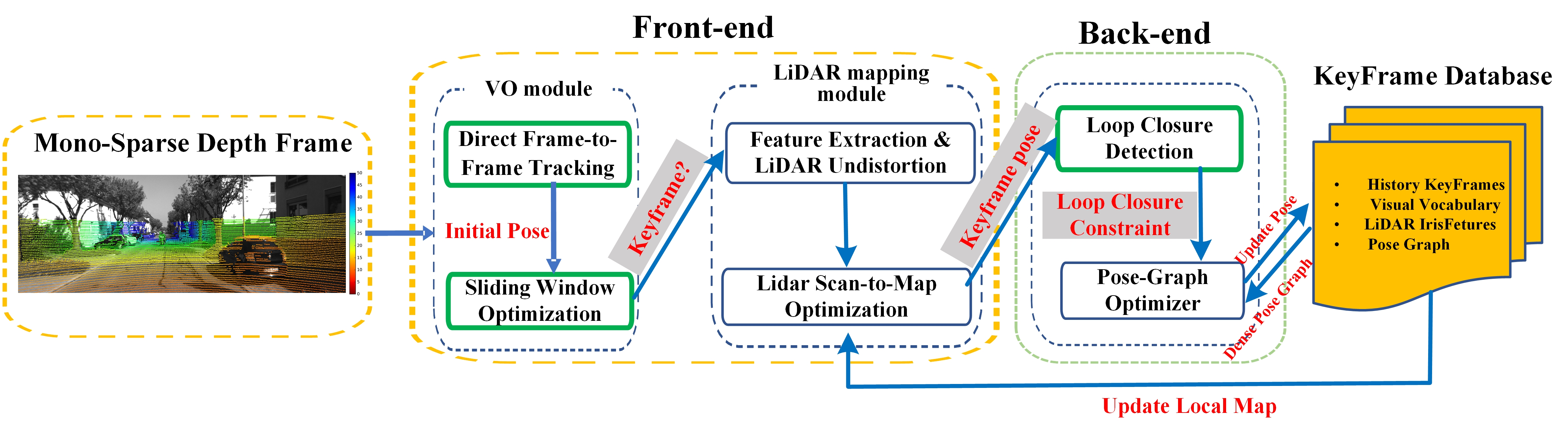
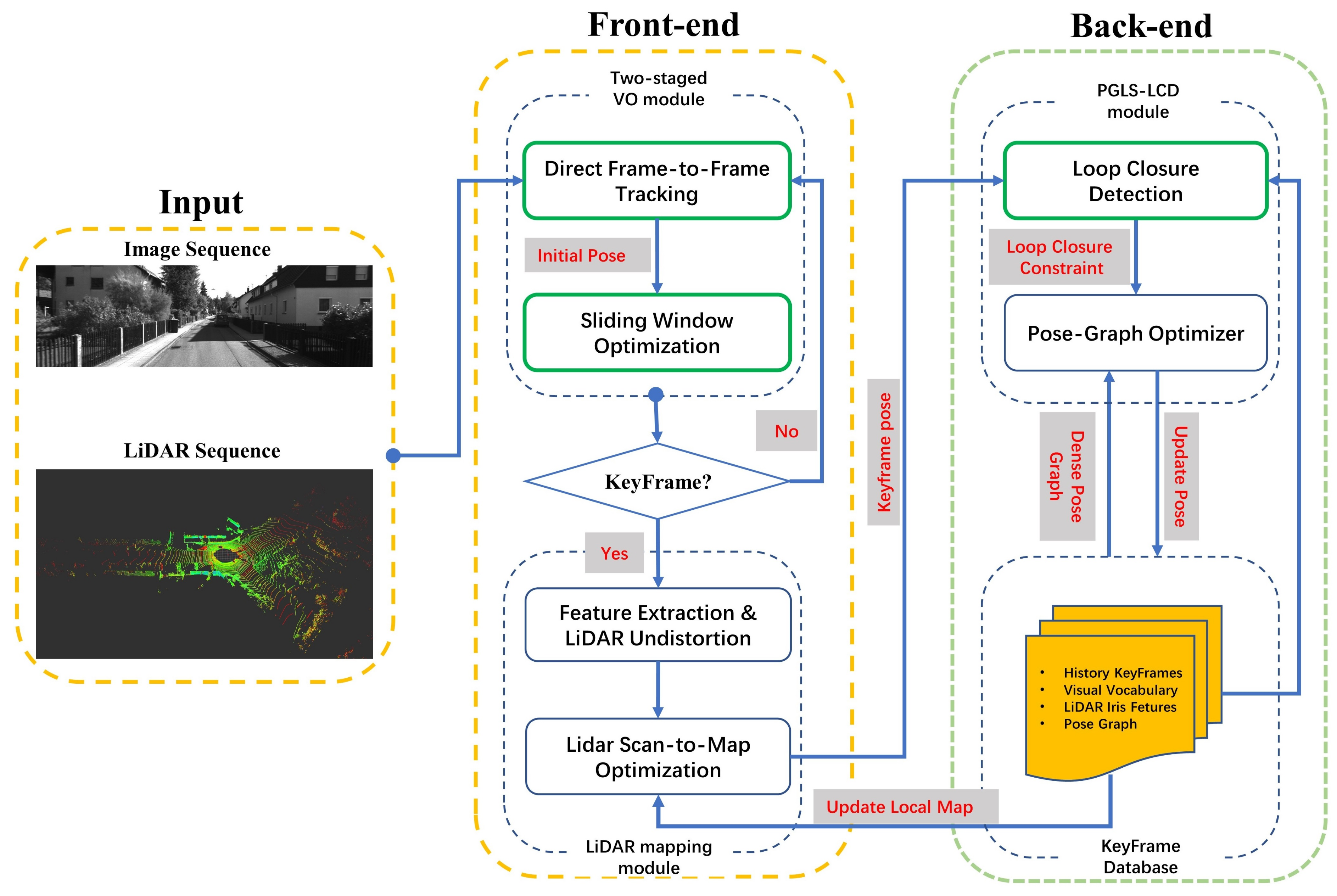
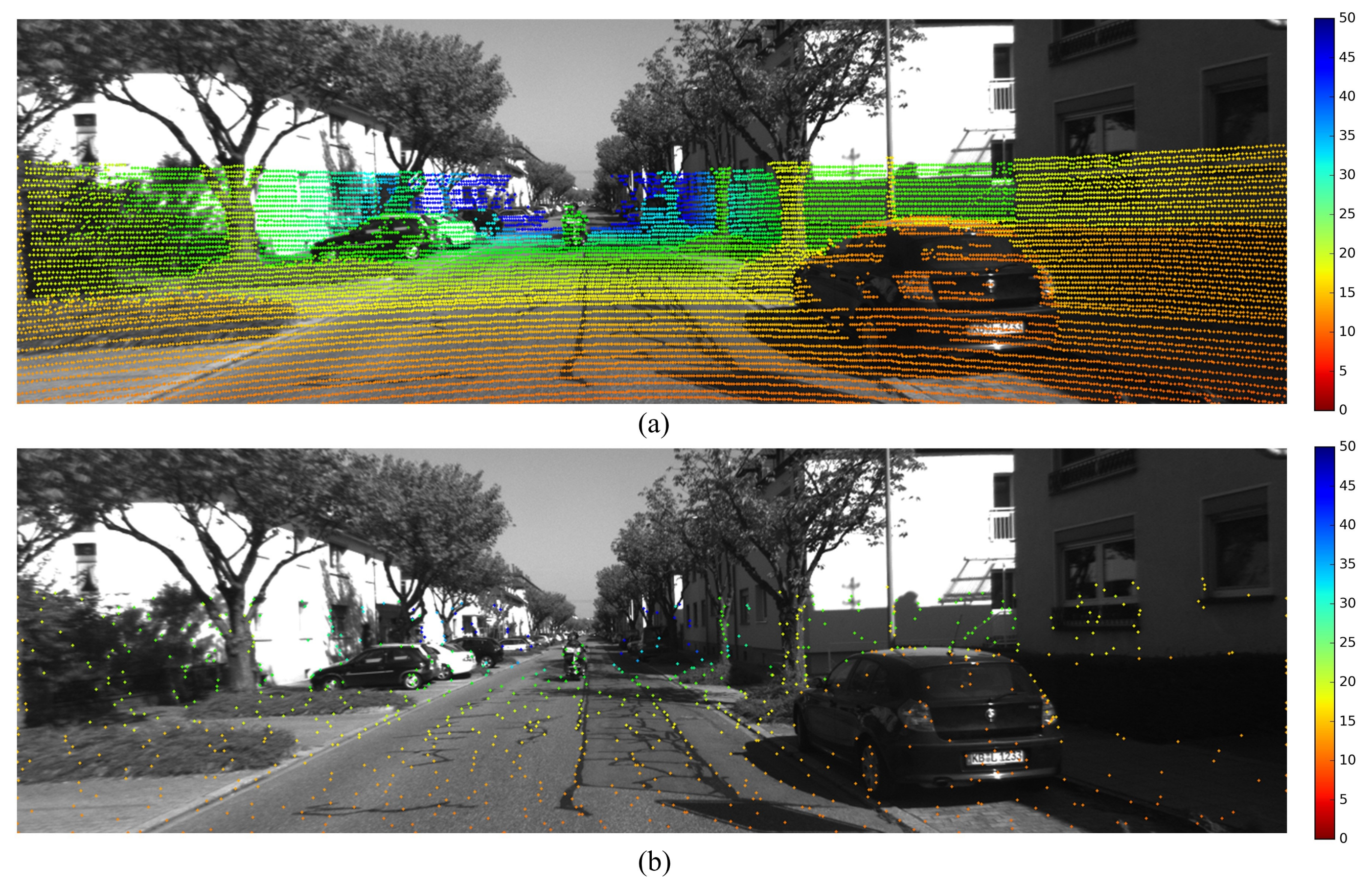
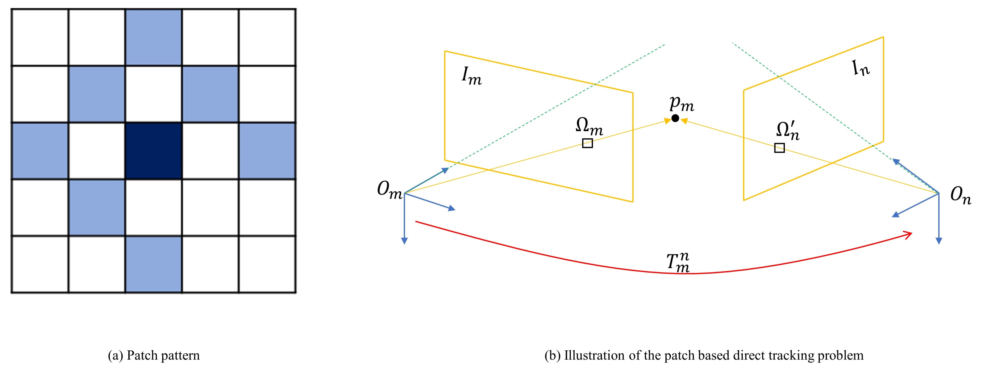
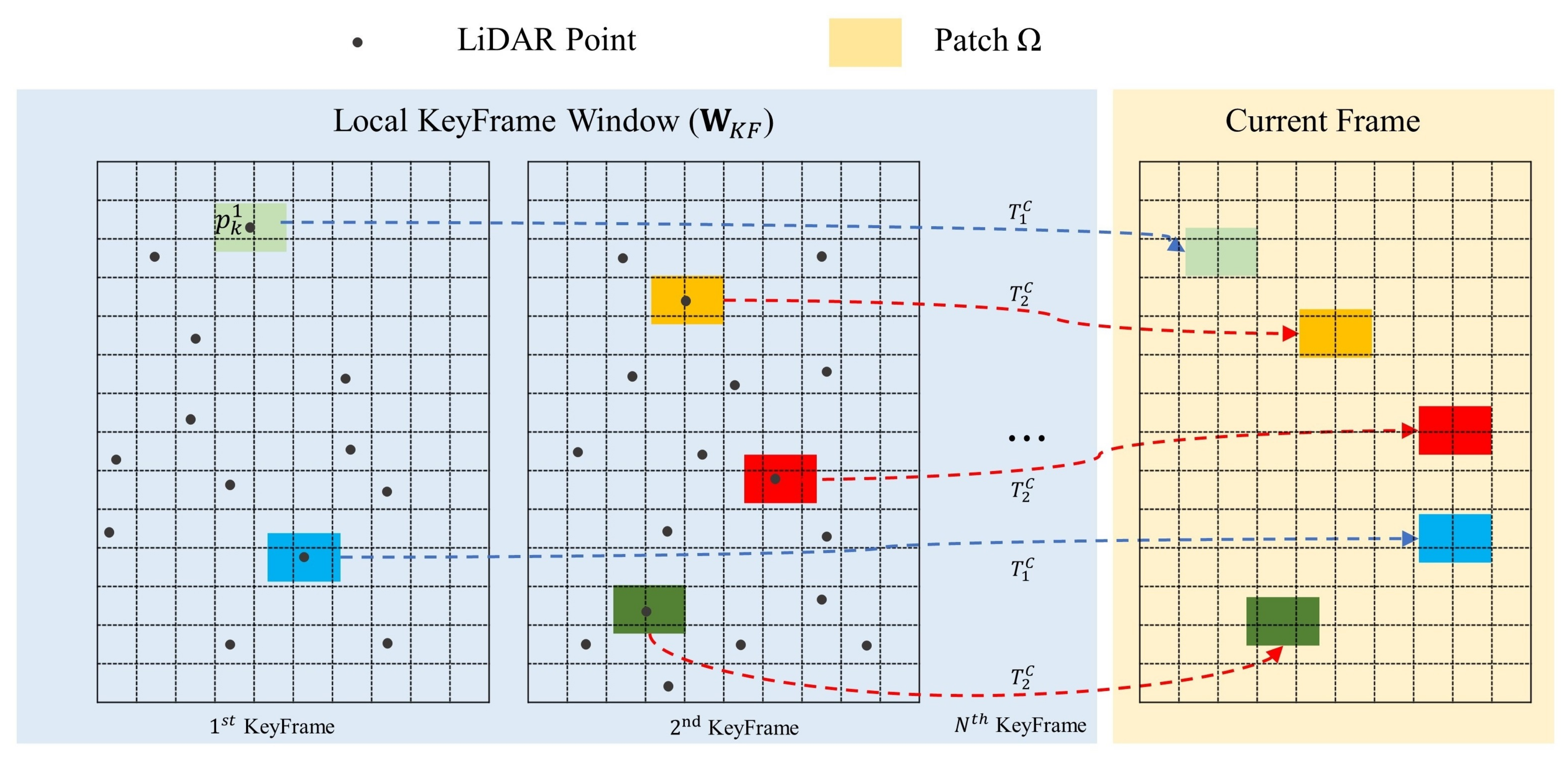
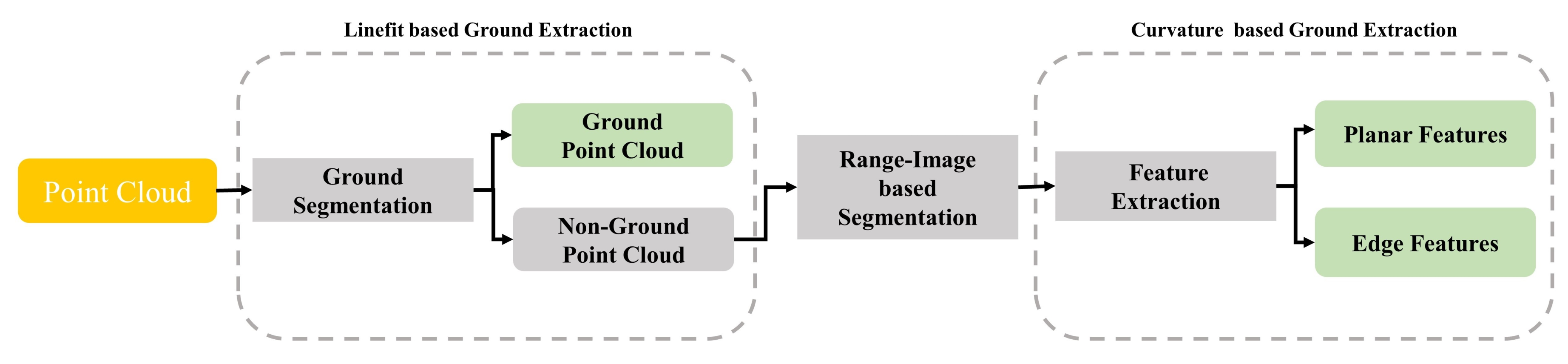
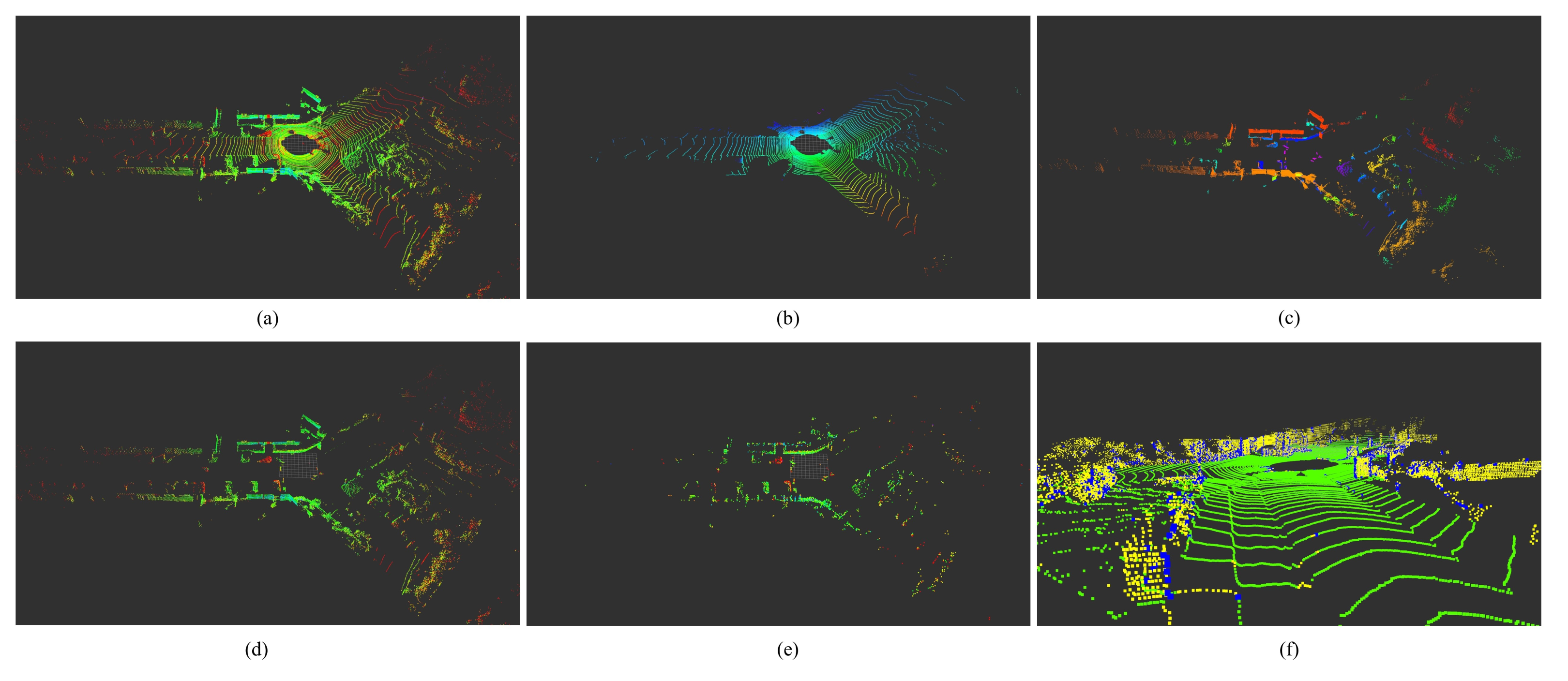
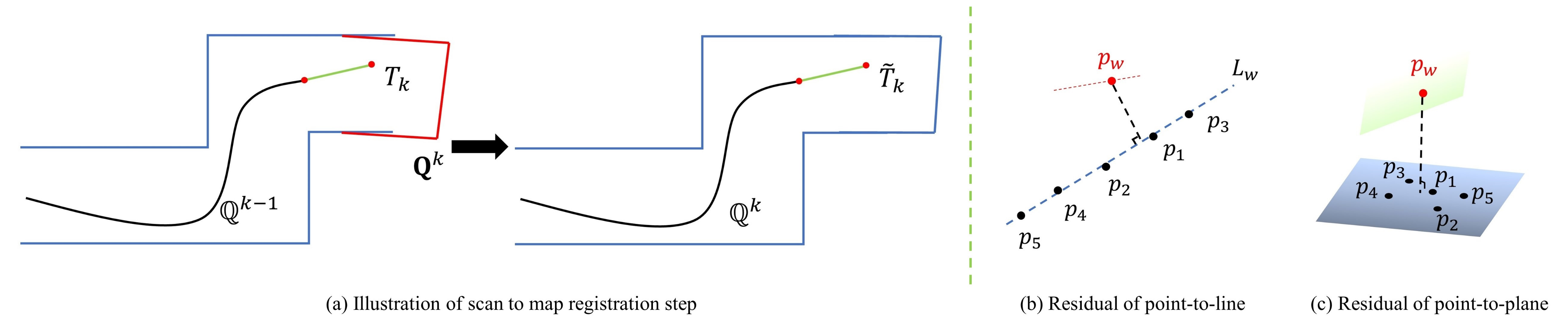
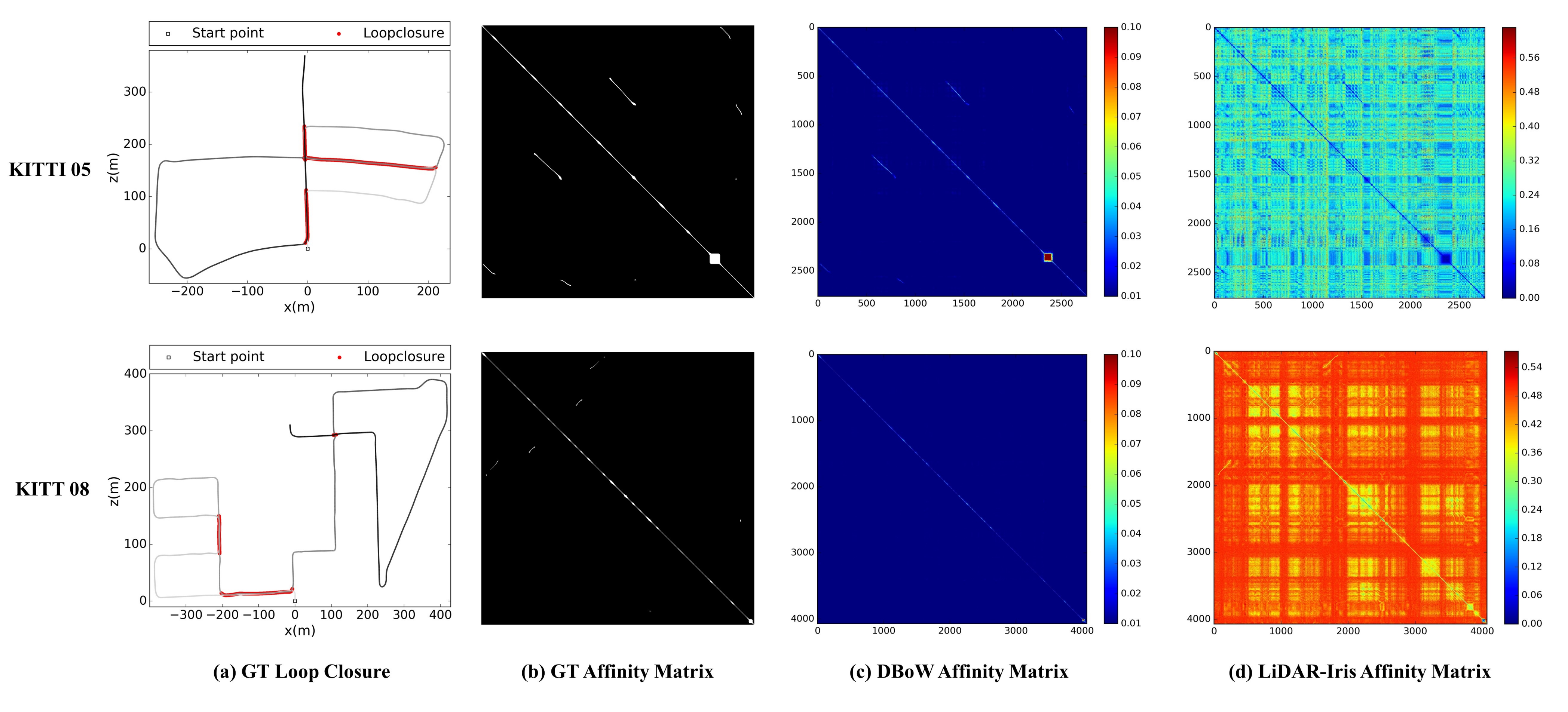
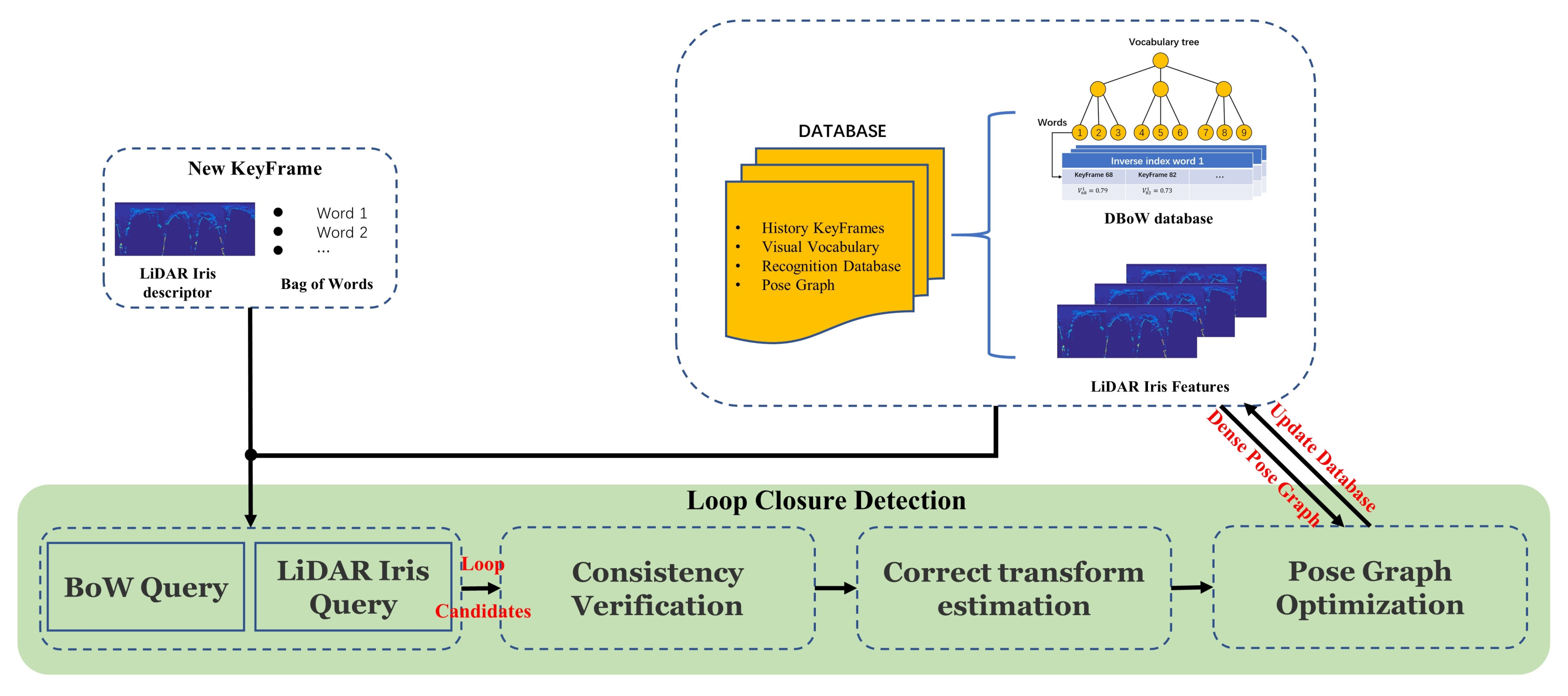
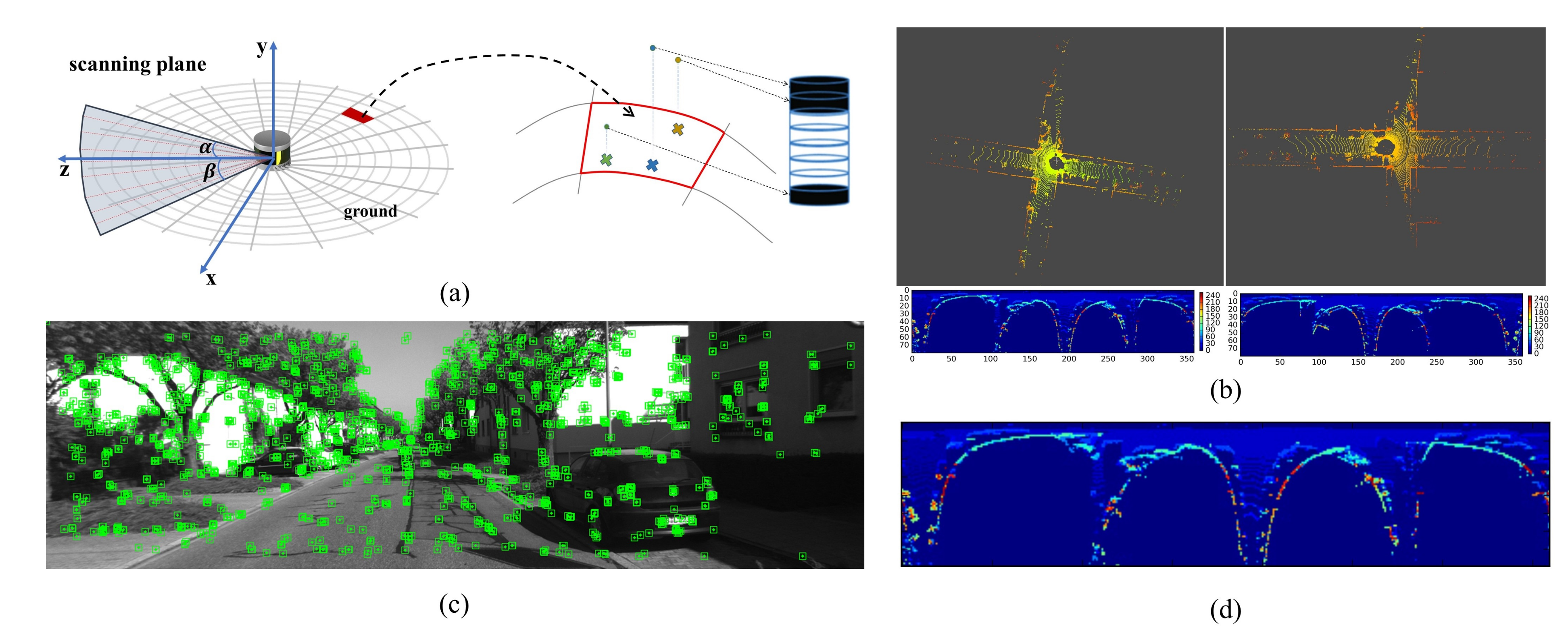
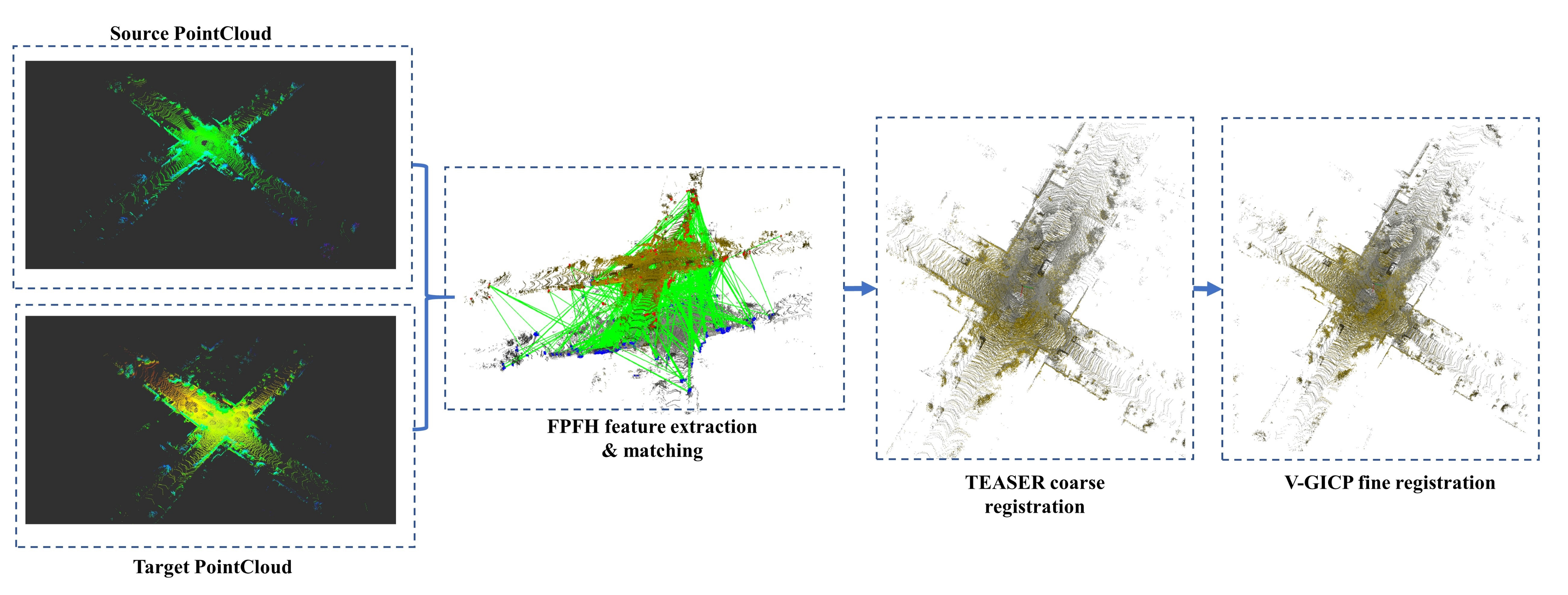
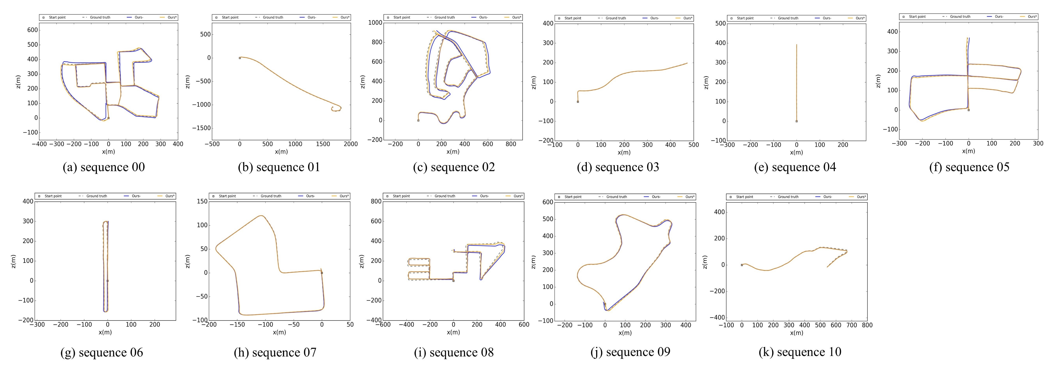
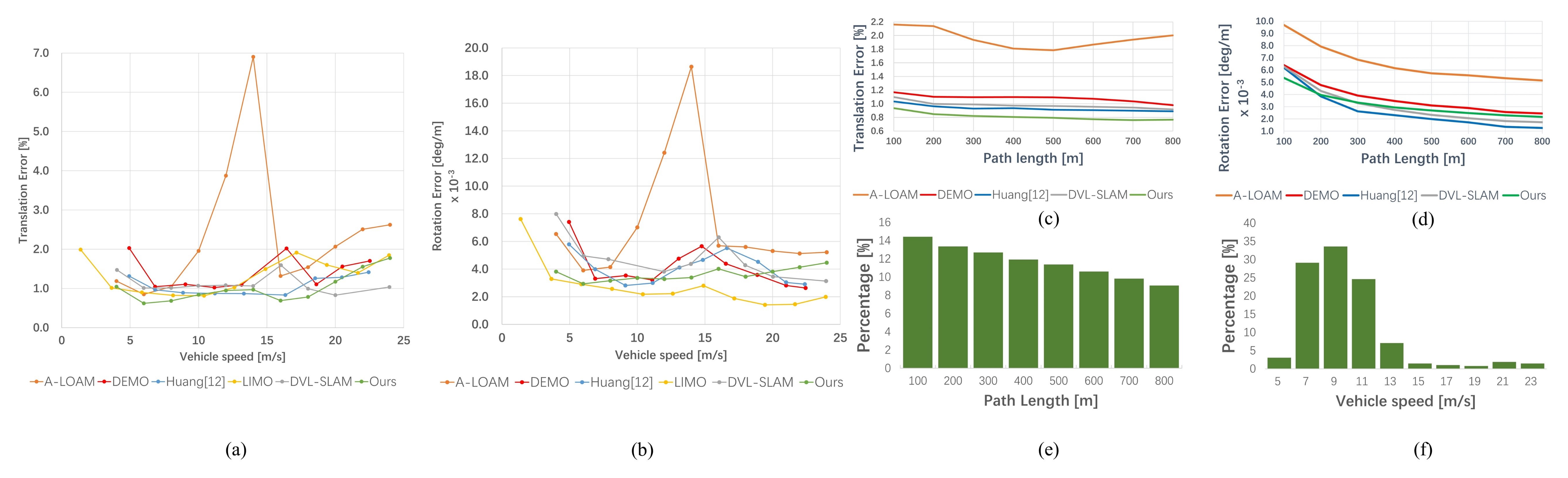
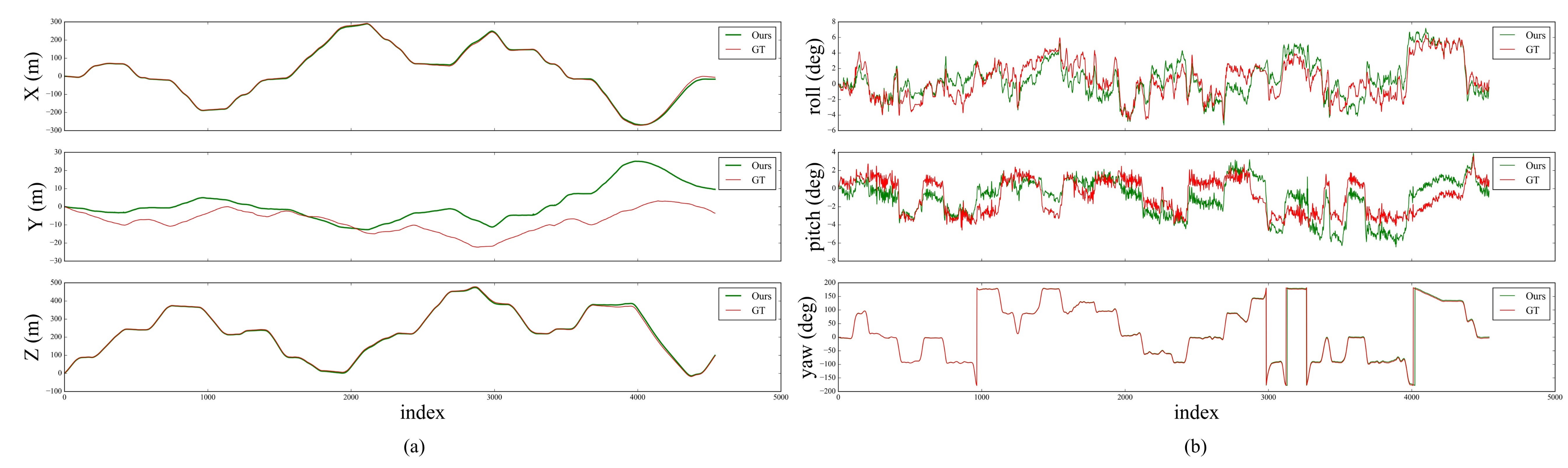
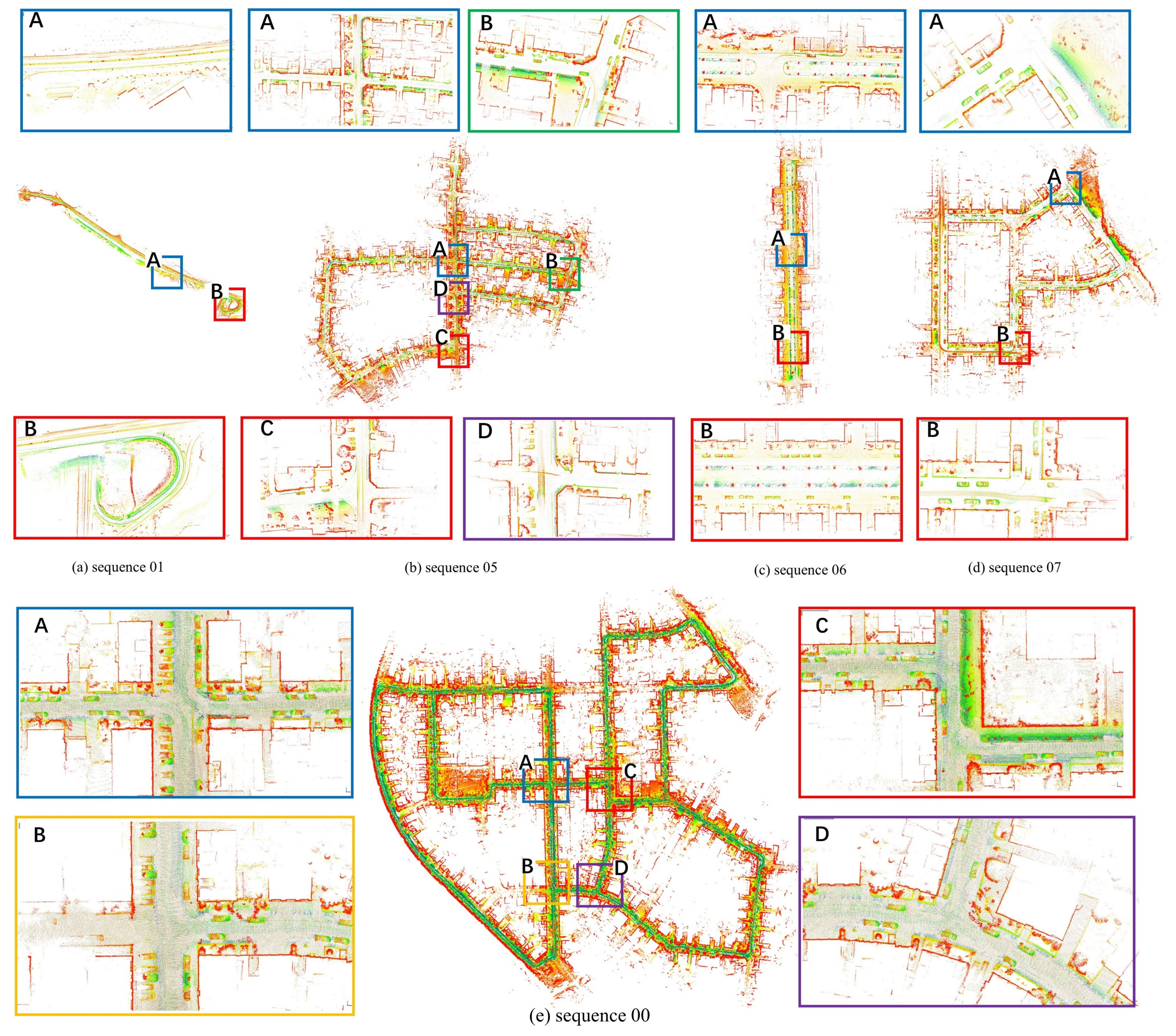
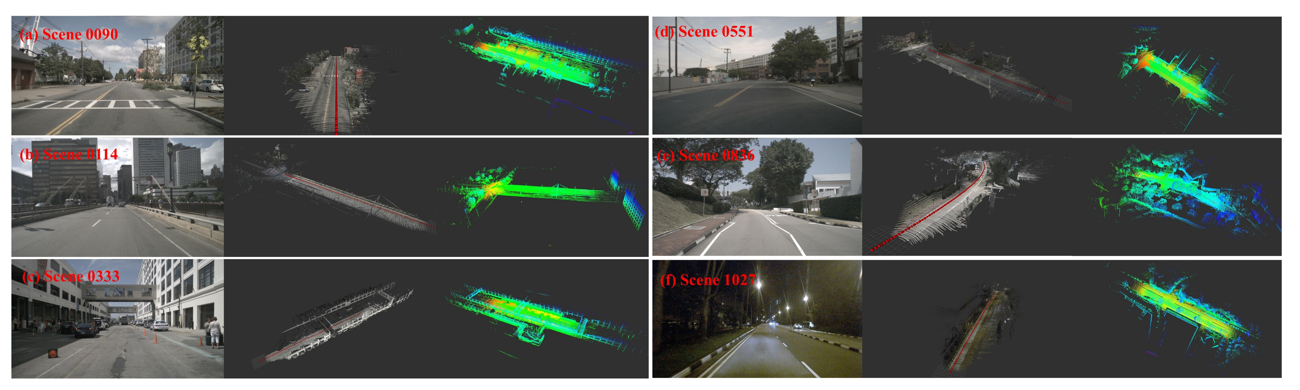
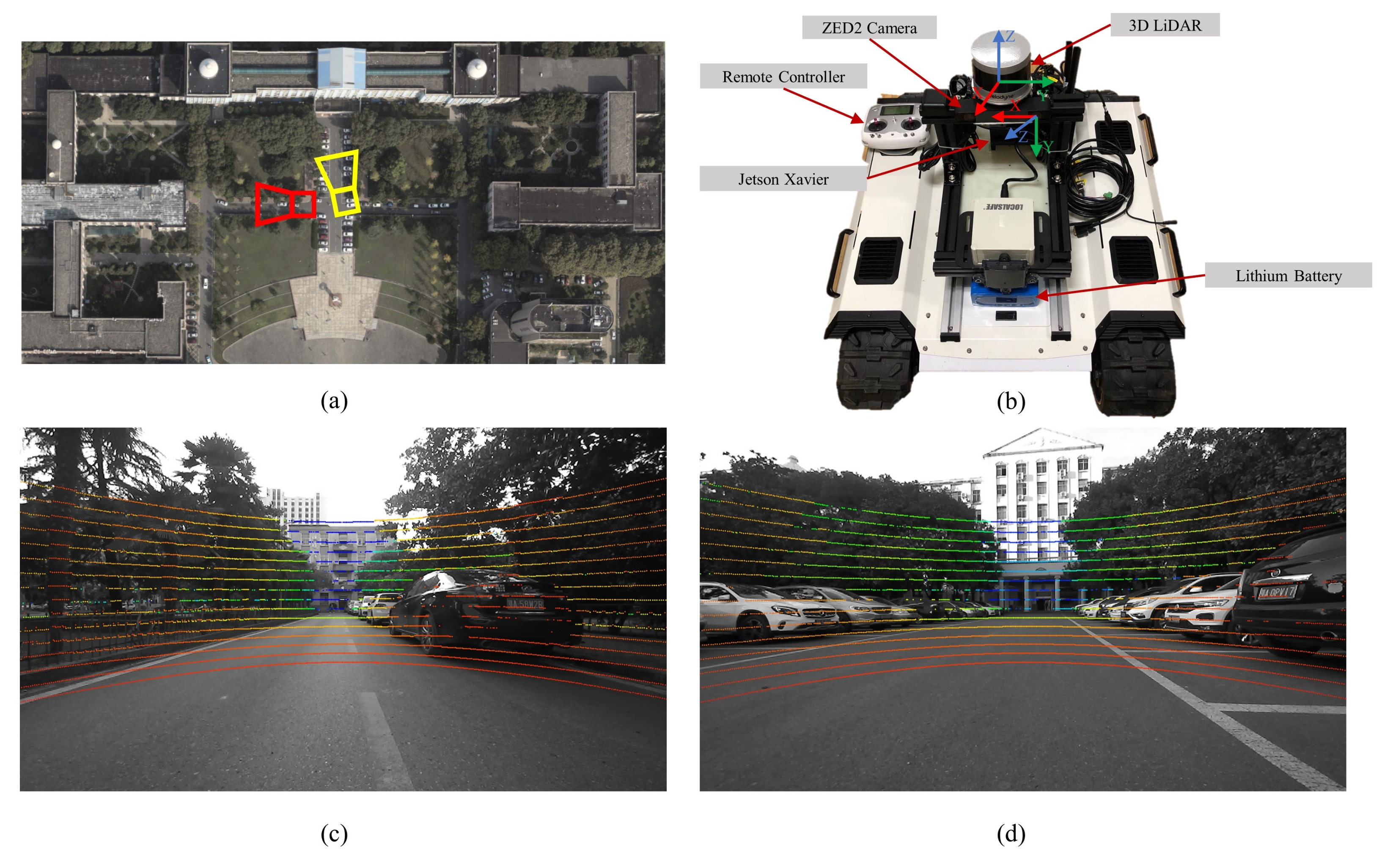
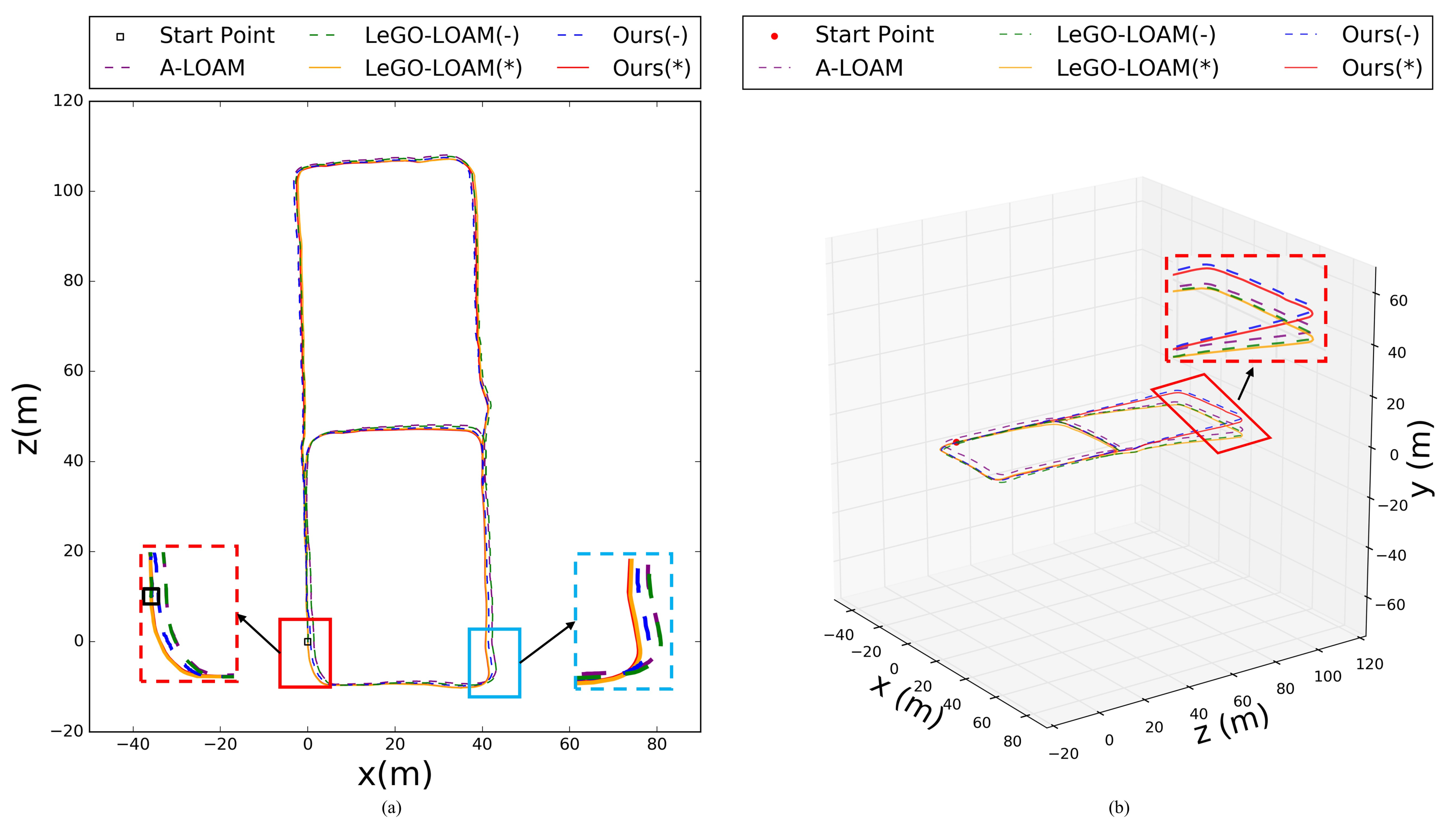
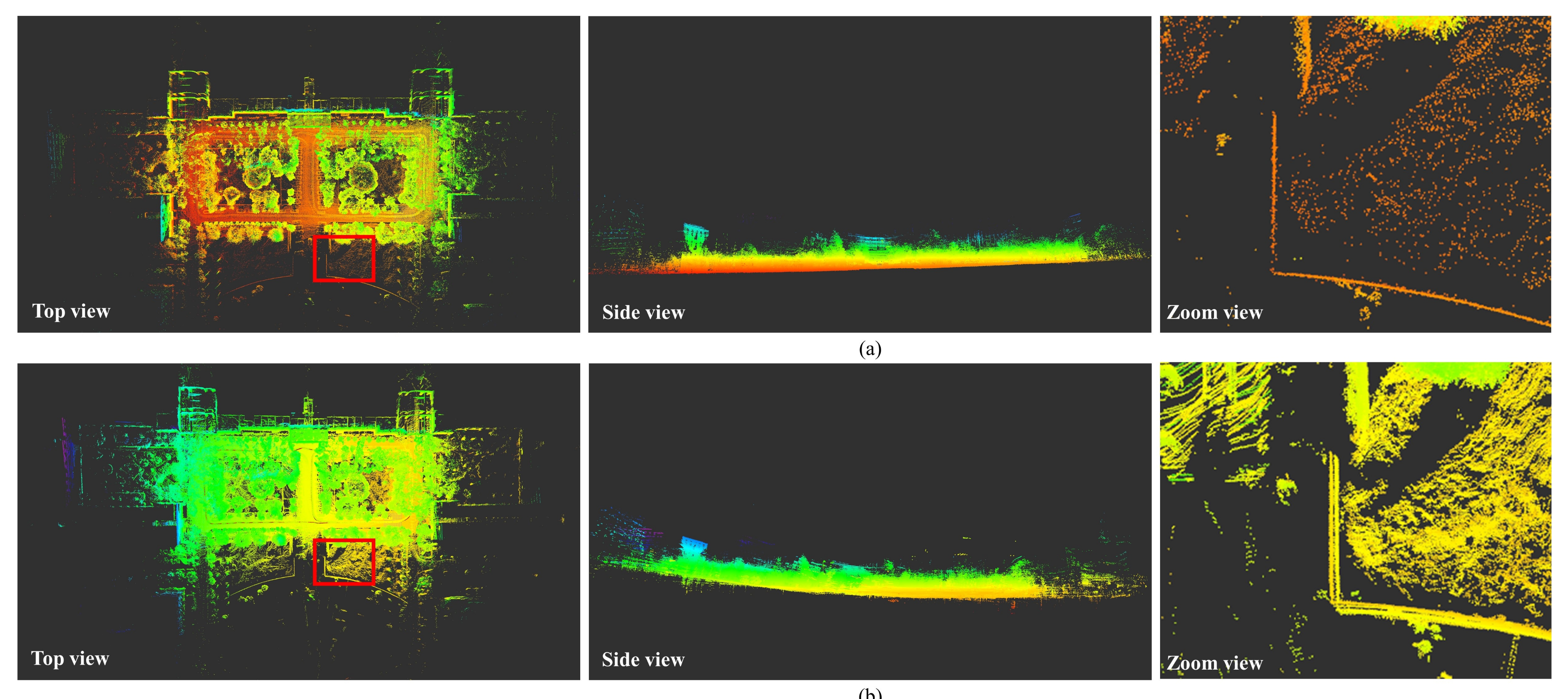
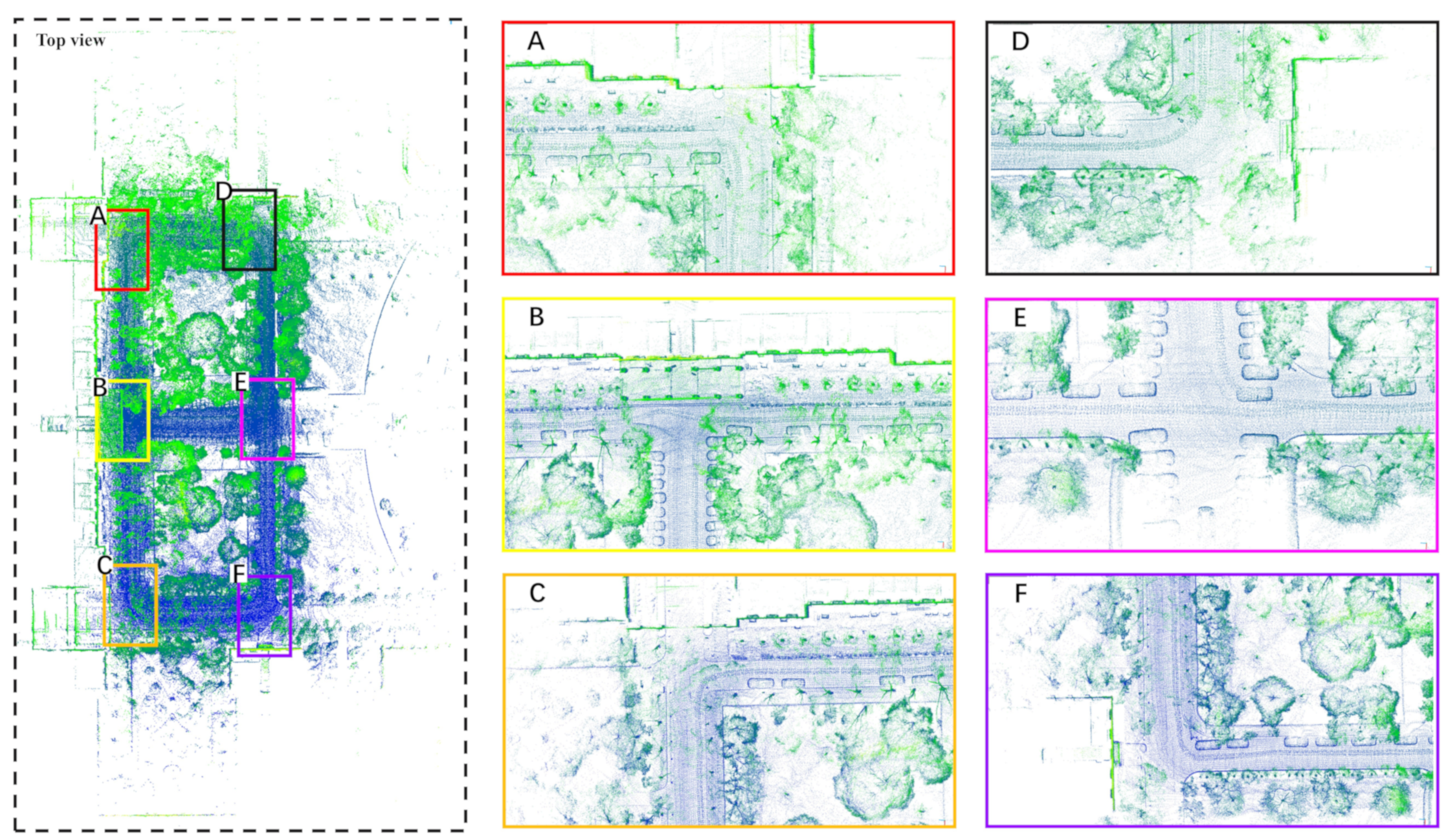
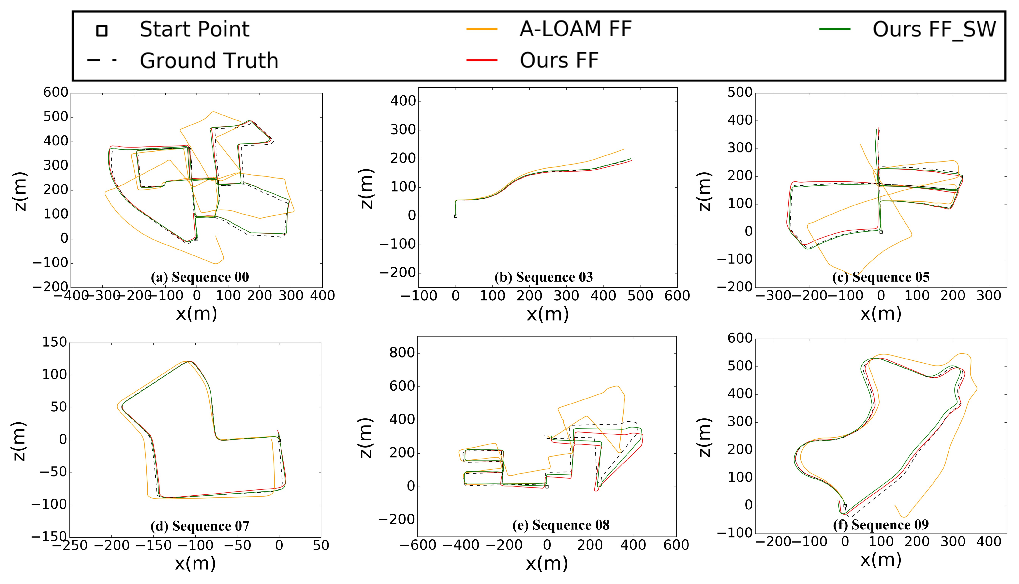
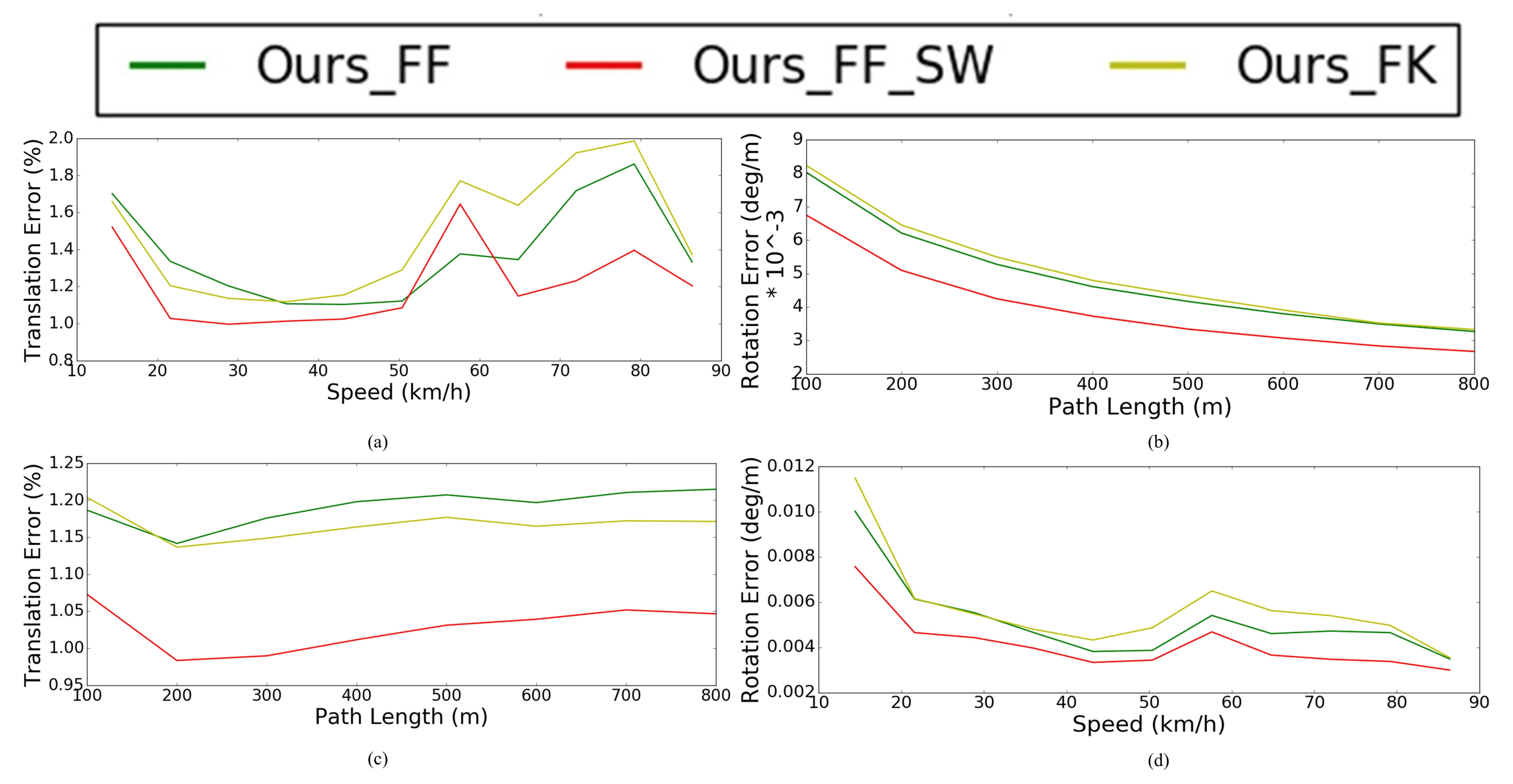
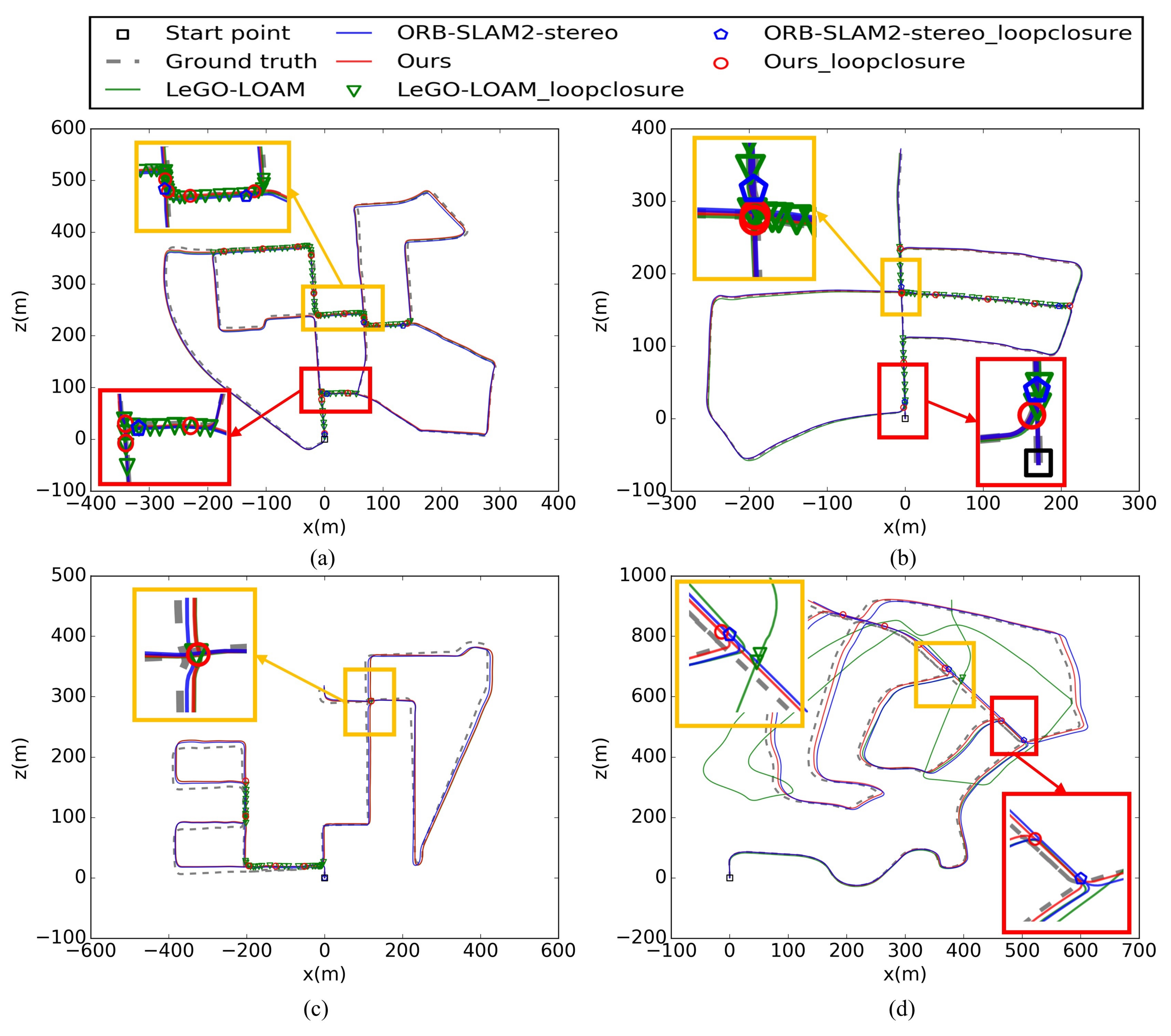
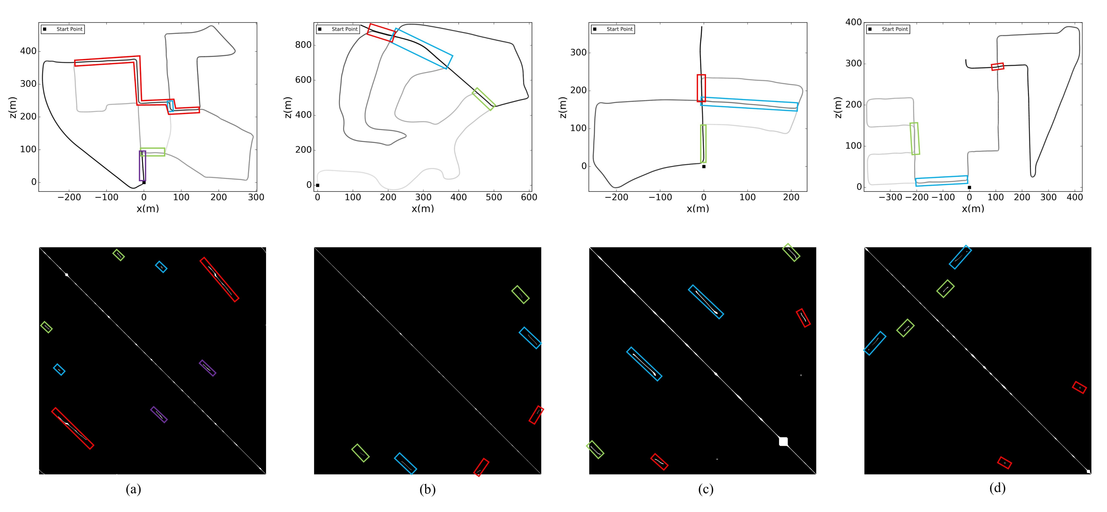
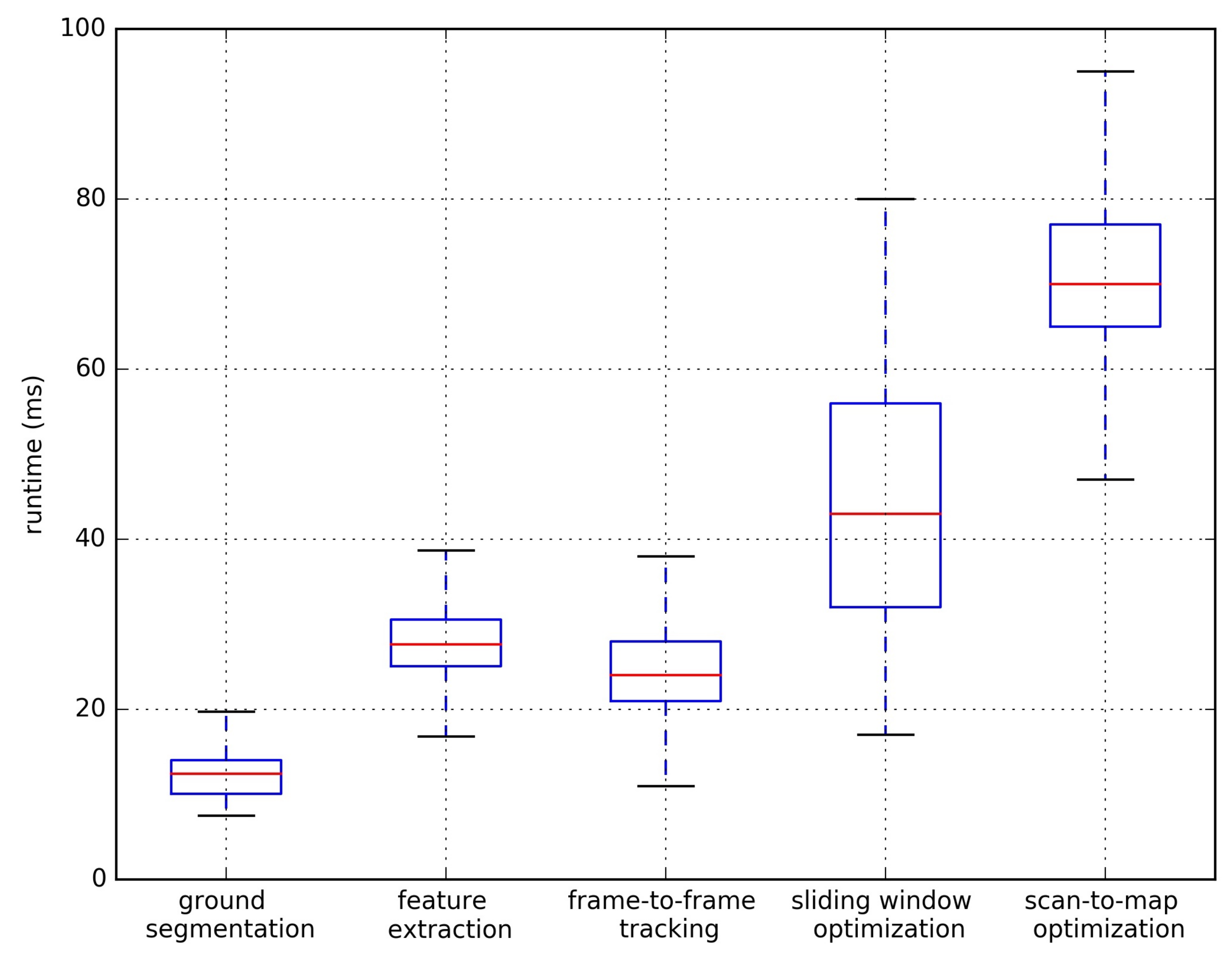
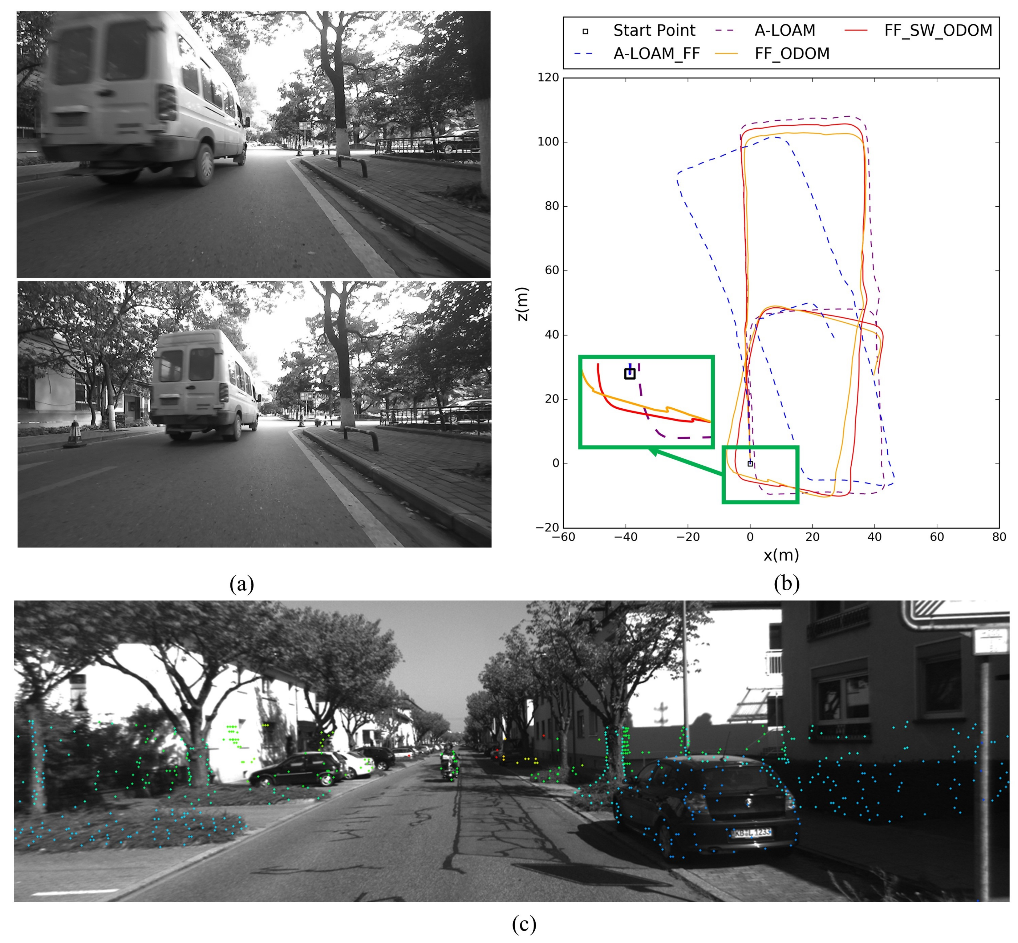
Table 1.
Parameters for DV-LOAM.
| Modules | Parameters | Description | KITTI | NuScenes | Ours |
|---|---|---|---|---|---|
| Visual Odometry | Number of image pyramid levels | 3 | 3 | 3 | |
| Max iteration of direct tracking in each level | 100 | 100 | 100 | ||
| Ration for keyframe creation | 0.7 | 0.8 | 0.8 | ||
| Time for keyframe creation (s) | 1.0 | 1.0 | 1.0 | ||
| Sliding window size (number of frames) | 3 | 3 | 5 | ||
| LiDAR Mapping | , , | The resolution of point cloud voxel downsample (m) | 0.4, 0.8, 0.8 | 0.4, 0.8, 0.8 | 0.3, 0.6, 0.6 |
| Loop Closing | The loop closure searching radius (m) | 10.0 | 10.0 | 10.0 | |
| The geometry consistency threshold | 40.0 | 40.0 | 40.0 | ||
| The suspend detection time after pose graph (s) optimization | 10.0 | 10.0 | 10.0 | ||
| The minimal gaps between candidate keyframe and last loop keyframe | 20 | 20 | 20 |
Table 2.
Translation error [%]/rotation error [deg/100 m] comparison of the proposed DV-LOAM with existing methods on the whole KITTI training dataset, where (-) represents without using loop closure and (*) represents using loop closure. Best results of (-) in relative translational error/relative rotational error are highlighted in red and blue, respectively.
| Seq. No | Path Len. (m) | Environment | LOAM [18] (-) | A-LOAM [25] (-) | LeGO- LOAM [19] (-) | DEMO [29] (-) | LIMO [27] (-) | Huang [35] (-) | DVL- SLAM [31] (-) | Ours (-) | Ours (*) |
|---|---|---|---|---|---|---|---|---|---|---|---|
| 00 | 3714 | Urban | 0.78/- | 0.87/0.36 | 1.51/0.70 | 1.05/- | 1.12/- | 0.99/- | 0.93/- | 0.65/0.30 | 0.66/0.30 |
| 01 | 4268 | Highway | 1.43/- | 2.64/0.55 | -/- | 1.87/- | 0.91/- | 1.87/- | 1.47/- | 1.74/0.43 | 1.74/0.43 |
| 02 | 5075 | Urban+Country | 0.92/- | 4.88/1.55 | 1.96/0.78 | 0.93/- | 1.38/- | 1.11/- | 0.97/0.33 | 0.84/0.36 | |
| 03 | 563 | Country | 0.86/- | 1.20/0.63 | 1.41/1.00 | 0.99/- | 0.65/- | 0.92/- | 0.85/0.48 | 0.85/0.48 | |
| 04 | 397 | Country | 0.71/- | 1.23/0.40 | 1.69/0.83 | 1.23/- | 0.53/- | 0.42/- | 0.67/- | 0.39/0.62 | 0.39/0.62 |
| 05 | 2223 | Urban | 0.57/- | 0.66/0.30 | 1.01/0.54 | 1.04/- | 0.72/- | 0.82/- | 0.54/0.30 | 0.43/0.22 | |
| 06 | 1239 | Urban | 0.65/- | 0.62/0.28 | 0.90/0.47 | 0.96/- | 0.61/- | 0.92/- | 0.65/0.33 | 0.70/0.33 | |
| 07 | 695 | Urban | 0.63/- | 0.58/0.43 | 0.81/0.56 | 1.16/- | 0.56/- | 1.26/- | 0.51/0.33 | 0.42/0.22 | |
| 08 | 3225 | Urban+Country | 1.12/- | 1.18/0.43 | 1.48/0.68 | 1.24/- | 1.27/- | 1.32/- | 0.89/0.32 | 0.93/0.27 | |
| 09 | 1717 | Urban+Country | 0.77/- | 1.10/0.45 | 1.57/0.80 | 1.17/- | 1.06/- | 0.66/- | 0.73/0.32 | 0.75/0.27 | |
| 10 | 919 | Urban+Country | 0.79/- | 1.46/0.53 | 1.81/0.85 | 1.14/- | 0.83/- | 0.70/- | 0.87/0.47 | 0.87/0.47 | |
| avg | 0.84/- | 1.49/0.53 | -/- | 1.14/0.49 | 0.93/0.26 | 0.94/0.36 | 0.98/0.40 | 0.80/0.38 | 0.78/0.36 |
Table 3.
Translation error [%]/rotation error [deg/100 m] comparison of the proposed DV-LOAM with existing methods on the NuScenes full dataset (v1.0) part 1. Best results in translational error/rotational error are highlighted in red and blue, respectively.
Table 3.
Translation error [%]/rotation error [deg/100 m] comparison of the proposed DV-LOAM with existing methods on the NuScenes full dataset (v1.0) part 1. Best results in translational error/rotational error are highlighted in red and blue, respectively.
| Scene No. | Environment | LeGO-LOAM [19] | A-LOAM [25] | Ours |
|---|---|---|---|---|
| 77–91 | Urban | 5.19/12.58 | 3.53/3.44 | 1.68/3.28 |
| 111–119 | Urban | 9.60/15.09 | 3.20/3.02 | 1.77/3.74 |
| 140–148 | Country | 8.90/16.32 | 5.71/5.38 | 3.85/3.69 |
| 265–266 | Urban | 3.55/11.46 | 5.74/4.83 | 1.54/3.45 |
| 279–282 | Country | 8.05/17.74 | 3.08/3.14 | 4.33/2.85 |
| 307–314 | Country | 9.03/26.23 | 4.40/4.83 | 4.10/7.0 |
| 333–343 | Urban | 10.70/16.46 | 5.51/4.27 | 1.98/3.3 |
| 547–551 | Urban | 6.34/13.28 | 5.42/2.73 | 1.24/2.17 |
| 602–604 | rain,Urban | 4.53/12.25 | 5.79/4.98 | 1.17/3.15 |
| 606–624 | rain,Urban | 6.97/18.78 | 5.81/4.72 | 1.57/4.00 |
| 833–842 | Country | 9.07/22.05 | 4.34/4.73 | 4.77/6.8 |
| 935–943 | Country | 12.12/21.80 | 5.63/4.18 | 5.37/3.71 |
| 1026–1043 | Country, Dark night | 13.79/20.34 | 3.28/4.06 | 6.04/4.72 |
| avg | 8.30/17.26 | 4.57/4.18 | 3.03/3.99 |
Table 4.
Translation error [%]/rotation error [deg/100 m] comparison of the different direct visual odometry with ICP-based LiDAR odometry on the whole KITTI training dataset.
Table 4.
Translation error [%]/rotation error [deg/100 m] comparison of the different direct visual odometry with ICP-based LiDAR odometry on the whole KITTI training dataset.
| Seq. No | Path Len. (m) | Environment | A-LOAM [25] FF | Ours FF | Ours FK-3 | Ours FK-5 | Ours FK-* | Ours FF-SW | Ours FF-SW-SM |
|---|---|---|---|---|---|---|---|---|---|
| 00 | 3714 | Urban | 4.11/1.70 | 1.08/0.52 | 1.00/0.50 | 1.67/0.88 | 1.12/0.55 | 0.95/0.43 | 0.65/0.30 |
| 01 | 4268 | Highway | 3.94/0.95 | 1.39/0.41 | -/- | -/- | 1.54/0.45 | 1.30/0.35 | 1.74/0.43 |
| 02 | 5075 | Urban+Country | 7.48/2.51 | 0.98/0.33 | 1.23/0.50 | 1.79/0.76 | 1.08/0.40 | 0.98/0.33 | 0.97/0.33 |
| 03 | 563 | Country | 4.54/2.15 | 1.19/0.48 | 1.14/0.53 | 1.53/1.12 | 1.08/0.50 | 0.95/0.88 | 0.85/0.48 |
| 04 | 397 | Country | 1.74/1.13 | 0.74/0.43 | 0.68/0.39 | 0.77/0.67 | 0.63/0.38 | 0.61/0.26 | 0.39/0.62 |
| 05 | 2223 | Urban | 4.13/1.75 | 1.20/0.58 | 0.88/0.42 | 0.96/0.50 | 0.98/0.48 | 0.79/0.36 | 0.54/0.30 |
| 06 | 1239 | Urban | 1.04/0.55 | 1.32/0.45 | 1.19/0.40 | 0.91/0.36 | 1.27/0.41 | 0.91/0.31 | 0.65/0.33 |
| 07 | 695 | Urban | 3.14/1.99 | 1.26/0.85 | 1.12/0.70 | 1.39/0.88 | 1.39/1.55 | 0.88/0.55 | 0.51/0.33 |
| 08 | 3225 | Urban+Country | 4.85/2.09 | 1.60/0.68 | 1.49/0.62 | 1.68/0.81 | 1.47/0.61 | 1.39/0.51 | 0.89/0.32 |
| 09 | 1717 | Urban+Country | 5.73/1.85 | 0.95/0.46 | 0.87/0.46 | 1.30/0.65 | 0.93/0.46 | 0.71/0.33 | 0.73/0.32 |
| 10 | 919 | Urban+Country | 3.61/1.78 | 1.05/0.49 | 0.96/0.42 | 1.29/0.66 | 0.87/0.43 | 0.77/0.36 | 0.87/0.47 |
| avg | 4.03/1.68 | 1.16/0.51 | -/- | -/- | 1.12/0.57 | 0.94/0.43 | 0.80/0.38 |
Table 5.
The loop closure precision and recall comparison with existing methods. The in Recall Rate represents the number of detected loop closure, and is the number of all existed loop closure segments. Best results are highlighted in bold.
Table 5.
The loop closure precision and recall comparison with existing methods. The in Recall Rate represents the number of detected loop closure, and is the number of all existed loop closure segments. Best results are highlighted in bold.
| Dateset | Approachs | Precision (%) | Recall Rate (/) |
|---|---|---|---|
| stereo ORB-SLAM2 | 100 | 4/4 | |
| sequence 00 | LeGO-LOAM | 100 | 4/4 |
| Ours | 100 | 4/4 | |
| stereo ORB-SLAM2 | 100 | 2/3 | |
| sequence 02 | LeGO-LOAM | 100 | 1/3 |
| Ours | 100 | 3/3 | |
| stereo ORB-SLAM2 | 100 | 3/3 | |
| sequence 05 | LeGO-LOAM | 100 | 3/3 |
| Ours | 100 | 3/3 | |
| stereo ORB-SLAM2 | 0 | 0/3 | |
| sequence 08 | LeGO-LOAM | 100 | 3/3 |
| Ours | 100 | 3/3 |
Table 6.
Average processing time of each module on the KITTI, nuScenes, and Our campus dataset.
| Modules | Sub Modules | KITTI (ms) | nuScenes (ms) | Our Campus (ms) |
|---|---|---|---|---|
| Visual Odometry | frame-to-frame tracking | 25.24 | 8.52 | 13.24 |
| sliding window optimization | 48.34 | 17.76 | 35.73 | |
| LiDAR Mapping | ground extraction | 12.19 | 8.57 | 9.46 |
| feature extraction | 27.84 | 11.30 | 10.23 | |
| scan-to-map optimization | 71.72 | 41.89 | 54.81 | |
| Loop Closing | loop candidates extraction | 3.98 | - | 3.24 |
| consistency verification | 110.37 | - | 102.53 | |
| pose graph optimization | 81.22 | - | 57.78 |
Table 7.
Translation error [%]/rotation error [deg/100 m] comparison of the different salient points selection trajectories in direct frame-to-frame visual-LiDAR odometry. Best results in translational error/rotational error are highlighted in red and blue, respectively.
Table 7.
Translation error [%]/rotation error [deg/100 m] comparison of the different salient points selection trajectories in direct frame-to-frame visual-LiDAR odometry. Best results in translational error/rotational error are highlighted in red and blue, respectively.
| 00 | 01 | 02 | 03 | 04 | 05 | 06 | 07 | 08 | 09 | 10 | avg | |
|---|---|---|---|---|---|---|---|---|---|---|---|---|
| FF(-) | 1.08/0.52 | 1.39/0.41 | 0.98/0.33 | 1.19/0.48 | 0.74/0.43 | 1.20/0.58 | 1.32/0.45 | 1.26/0.85 | 1.60/0.68 | 0.95/0.46 | 1.05/0.49 | 1.16/0.51 |
| FF(*) | 1.01/0.50 | 1.29/0.40 | 0.96/0.32 | 1.08/0.46 | 0.77/0.41 | 1.06/0.50 | 0.97/0.42 | 1.29/0.93 | 1.60/0.68 | 1.02/0.46 | 1.11/0.46 | 1.11/0.50 |
Publisher’s Note: MDPI stays neutral with regard to jurisdictional claims in published maps and institutional affiliations. |
© 2021 by the authors. Licensee MDPI, Basel, Switzerland. This article is an open access article distributed under the terms and conditions of the Creative Commons Attribution (CC BY) license (https://creativecommons.org/licenses/by/4.0/).
Share and Cite
MDPI and ACS Style
Wang, W.; Liu, J.; Wang, C.; Luo, B.; Zhang, C. DV-LOAM: Direct Visual LiDAR Odometry and Mapping. Remote Sens. 2021, 13, 3340. https://0-doi-org.brum.beds.ac.uk/10.3390/rs13163340
AMA Style
Wang W, Liu J, Wang C, Luo B, Zhang C. DV-LOAM: Direct Visual LiDAR Odometry and Mapping. Remote Sensing. 2021; 13(16):3340. https://0-doi-org.brum.beds.ac.uk/10.3390/rs13163340
Chicago/Turabian StyleWang, Wei, Jun Liu, Chenjie Wang, Bin Luo, and Cheng Zhang. 2021. "DV-LOAM: Direct Visual LiDAR Odometry and Mapping" Remote Sensing 13, no. 16: 3340. https://0-doi-org.brum.beds.ac.uk/10.3390/rs13163340
Note that from the first issue of 2016, this journal uses article numbers instead of page numbers. See further details here.