Article

Mapping Daily Evapotranspiration at Field Scale Using the Harmonized Landsat and Sentinel-2 Dataset, with Sharpened VIIRS as a Sentinel-2 Thermal Proxy

1
Hydrology and Remote Sensing Laboratory, USDA-ARS, 10300 Baltimore Avenue, Beltsville, MD 20705, USA
2
Earth Science Office, Marshall Space Flight Center, NASA, Huntsville, AL 35805, USA
3
Earth System Science Interdisciplinary Center, University of Maryland, College Park, MD 20742, USA
*
Author to whom correspondence should be addressed.
Remote Sens. 2021, 13(17), 3420; https://0-doi-org.brum.beds.ac.uk/10.3390/rs13173420
Submission received: 6 July 2021 / Revised: 18 August 2021 / Accepted: 24 August 2021 / Published: 28 August 2021
(This article belongs to the Special Issue Remote Sensing-Based Evapotranspiration Models)

Abstract

:
Accurate and frequent monitoring of evapotranspiration (ET) at sub-field scales can provide valuable information for agricultural water management, quantifying crop water use and stress toward the goal of increasing crop water use efficiency and production. Using land-surface temperature (LST) data retrieved from Landsat thermal infrared (TIR) imagery, along with surface reflectance data describing albedo and vegetation cover fraction, surface energy balance models can generate ET maps down to a 30 m spatial resolution. However, the temporal sampling by such maps can be limited by the relatively infrequent revisit period of Landsat data (8 days for combined Landsats 7 and 8), especially in cloudy areas experiencing rapid changes in moisture status. The Sentinel-2 (S2) satellites, as a good complement to the Landsat system, provide surface reflectance data at 10–20 m spatial resolution and 5 day revisit period but do not have a thermal sensor. On the other hand, the Visible Infrared Imaging Radiometer Suite (VIIRS) provides TIR data on a near-daily basis with 375 m resolution, which can be refined through thermal sharpening using S2 reflectances. This study assesses the utility of augmenting the Harmonized Landsat and Sentinel-2 (HLS) dataset with S2-sharpened VIIRS as a thermal proxy source on S2 overpass days, enabling 30 m ET mapping at a potential combined frequency of 2–3 days (including Landsat). The value added by including VIIRS-S2 is assessed both retrospectively and operationally in comparison with flux tower observations collected from several U.S. agricultural sites covering a range of crop types. In particular, we evaluate the performance of VIIRS-S2 ET estimates as a function of VIIRS view angle and cloud masking approach. VIIRS-S2 ET retrievals (MAE of 0.49 mm d−1 against observations) generally show comparable accuracy to Landsat ET (0.45 mm d−1) on days of commensurate overpass, but with decreasing performance at large VIIRS view angles. Low-quality VIIRS-S2 ET retrievals linked to imperfect VIIRS/S2 cloud masking are also discussed, and caution is required when applying such data for generating ET timeseries. Fused daily ET time series benefited during the peak growing season from the improved multi-source temporal sampling afforded by VIIRS-S2, particularly in cloudy regions and over surfaces with rapidly changing vegetation conditions, and value added for real-time monitoring applications is discussed. This work demonstrates the utility and feasibility of augmenting the HLS dataset with sharpened VIIRS TIR imagery on S2 overpass dates for generating high spatiotemporal resolution ET products.

Graphical Abstract

1. Introduction

Efficient use of agricultural water resources is becoming increasingly important for sustainable agricultural water management and global food production [1]. Evapotranspiration (ET), one of the major forms of water loss in agricultural landscapes, plays a crucial role in describing crop water use and soil moisture status [2]. Accurate monitoring of ET at field or sub-field scales can be used to identify crop stress and increase crop water use efficiency, thereby improving potential for crop production in water-limited regions. Thermal remote sensing has become one of the most effective techniques for ET mapping, complementing conventional point-based observational methods including eddy covariance, Bowen ratio (BR) and lysimeters [3]. Field measurements of ET are sparse and localized, and thus of limited use for operational applications, while ET models developed on remote sensing data are more suited for mapping the spatial distribution of ET at both field and regional scales [4,5,6,7,8]. Over the past few decades, several thermal satellite-based approaches have been developed and widely applied, including the Surface Energy Balance Algorithm for Land (SEBAL) [9], the Mapping Evapotranspiration with Internalized Calibration (METRIC) [10], the Operational Simplified Surface Energy Balance (SSEBop) [11] and the Atmosphere-Land Exchange Inverse model (ALEXI) [12,13] and its associated flux disaggregation technique (DisALEXI) [14,15]. These remote sensing approaches use land surface temperature (LST) retrieved from satellite thermal radiances along with other land surface characteristics such as surface albedo and leaf area index (LAI) or other vegetation indices to estimate ET via surface energy balance or within-scene scaling [15,16,17,18].
The Landsat imaging system, with sensors covering the spectrum from visible, near-infrared, shortwave infrared to TIR (thermal infrared) and at spatial resolutions from 30–120 m, is a gold standard for field-scale ET monitoring [10,19]. However, the relatively low revisit frequency of 16 days for a single Landsat system or 8 days for two combined Landsat systems (Table 1) limits its applicability for routine generation of daily ET estimates at field scales, with cloud cover further reducing the actual data availability [19,20,21]. Moderate-resolution sensors such as the Moderate Resolution Imaging Spectroradiometer (MODIS) and the Visible Infrared Imaging Radiometer Suite (VIIRS) can provide valuable information about moisture dynamics at coarser scales (~500 m) on a near-daily basis. To generate spatially and temporally high-resolution ET products, spatiotemporal image fusion techniques such as Spatial and Temporal Adaptive Reflectance Fusion Model (STARFM) [22] have been employed to produce 30 m daily ET estimates from MODIS and Landsat retrievals with mean absolute errors (MAE) lower than 1 mm d−1 over a range of land cover types [23,24,25,26,27].
While data fusion provides a valuable means for temporal interpolation, the accuracy or the resulting daily 30 m timeseries is highly dependent on the frequency and quality of clear-sky Landsat-scale ET imagery. In addition, performance for real-time applications may be further limited by latencies in Landsat product availability, and the need for extrapolation beyond the last available Landsat overpass to the current date. The fusion of ET timeseries from Landsat 8 and MODIS for operational applications was tested by [28]. They found that the 16 day revisit interval of Landsat 8, together with the 21.6 day latency, was not sufficient to effectively capture vegetation response to stress onset and suggested that the integration of data from multiple Landsat-like sensor platforms and a reduction in data latency could be useful.
As a test of multi-source ET mapping capabilities, reference [29] incorporated thermal imaging from the ECOsystem Spaceborne Thermal Radiometer Experiment on Space Station (ECOSTRESS), with ~70 m spatial resolution and an average 4 day revisit cycle, into the ET fusion system. Since ECOSTRESS is a thermal-only sensor, VSWIR (visible to shortwave infrared bands) data from the closest Landsat overpass date were used to supply albedo and LAI inputs to the ET modeling system. In comparison with flux tower observations, they demonstrated that fusion of the combined dataset of ECOSTRESS and Landsat (labeled as Landsat + ECOSTRESS fusion) showed improved performance over Landsat-only fusion, particularly over sites impacted by frequent cloud cover. While ECOSTRESS TIR and Landsat VSWIR inputs could in most cases be successfully combined within the energy balance model, Landsat ET retrievals were superior due to better inter-band registration. Furthermore, significant temporal separation between Landsat VSWIR and ECOSTRESS TIR acquisitions can lead to discrepancies between LST and LAI/albedo inputs and impose a source of error in the retrieved ET [29].
The Sentinel-2 (S2) satellite series (A and B), initially launched in 2015, provides surface reflectance (SR) data at 10–20 m spatial resolution with a 5 day combined repeat frequency (Table 1). Given the similarity with Landsat spectral bands and spatial scale, there has been a strong emphasis put on exploiting these data in combination to enhance temporal sampling. NASA’s Harmonized Landsat and Sentinel-2 (HLS) dataset provides a unified collection of SR data acquired by Landsat 8 and S2 [30], with a combined effective revisit of 3–4 days. The high temporal resolution of HLS makes it attractive for ET mapping at field scales; however, S2 does not collect the TIR data required for surface energy balance. Some studies have used S2 SR data to sharpen Sentinel-3 (S3, launched 2016) 1 km resolution TIR images for modeling daily ET [31]. However, VIIRS (see Table 1), the follow-on instrument to MODIS, includes an I5 TIR band at 375 m that is closer in resolution to S2 and has been collecting TIR data with near-daily temporal frequency since 2013 [32,33]. Reference [34] demonstrated that S2 SR data from the HLS-S30 product could be effectively used to sharpen VIIRS TIR data to 30 m resolution, facilitating VIIRS and S2 combined 30 m ET retrieval. Selecting VIIRS data on S2 overpass days relieves the issue of temporal separation encountered using Landsat VSWIR and ECOSTRESS TIR data [29].
Given these considerations, in this study we aim to evaluate the value of adding VIIRS and S2 data to the existing Landsat-only ET fusion framework. We first compare the VIIRS and S2 combined 30 m ET retrievals (labeled as VIIRS-S2 ET) with Landsat retrievals for consistency both spatially and temporally. Cases with poor VIIRS-based ET retrievals are investigated, specifically focusing on the impact of view angles (range of ±~70°; Table 1) and cloud masks on VIIRS LST. Both Landsat 30 m ET retrievals only (Landsat-only fusion) and Landsat and VIIRS-S2 ET retrievals together (labeled as Landsat + VIIRS-S2 fusion) are fused with MODIS 500 m daily ET estimates to generate two 30 m daily ET datacubes. The added value of additional VIIRS-S2 temporal sampling for both retrospective and real-time ET mapping applications is evaluated using flux measurements from 11 tower sites across a range of crop types in the U.S. Furthermore, we assess the capability of each data stream, alone and in combination, in establishing the temporal behavior of ET during periods of rapid change (e.g., rainfall events, flash drought, green-up, and senescence).

2. Methods

The multi-scale ALEXI and DisALEXI energy balance modeling system was used to generate consistent ET layers from multi-source thermal and SR inputs. In this system, daily regional ALEXI ET at 4 km resolution, developed from continental-scale geostationary satellite imagery, are spatially disaggregated (DisALEXI) using higher-resolution LST and SR data from Landsat and VIIRS-S2 as input, as well as moderate-resolution data from MODIS used as the fusion backbone. A data mining sharpener (DMS) approach is employed to spatially sharpen the Landsat, VIIRS, and MODIS LST inputs to DisALEXI, and the output timeseries are subsequently fused to produce daily ET at 30 m resolution (See Figure 1). A schematic overview of the ET processing is illustrated in Figure 1 and the major components are detailed in the following sections.

2.1. Data Mining Sharpener (DMS)

The spatial resolution of land surface temperature (LST) data retrieved from thermal infrared (TIR) satellite sensors is typically coarser than that of the surface reflectance data collected in VSWIR bands on the same platform. For instance, the resolution of Landsat 8 and MODIS VSWIR bands are 30 m and 250–500 m, while the nominal resolution of TIR sensors in these systems are 100 m and 1 km, respectively (Table 1). For physically based energy balance models such as ALEXI/DisALEXI, it is critical that LST, albedo and LAI inputs are at a consistent spatial resolution. Rather than degrading the VSWIR inputs to TIR resolution, a thermal band imagery sharpening technique known as the data mining sharpener (DMS) approach [35] has been used to sharpen both Landsat and MODIS LST data to the resolution of their corresponding VSWIR bands. The DMS approach employs the cubist regression tree method to build non-linear relationships between SR and LST at LST coarse resolution and then uses these relationships to predict LST at finer SR resolution using SR data as inputs. The final critical step of the sharpening process, referred to as energy conservation (EC), is to redistribute the residuals between the original and predicted LST at the coarse resolution to the sharpened LST to ensure that it reaggregates to the original LST field at some spatial scale. For Landsat 8 and MODIS TIR sharpening, the EC size scale used in DMS is 90 m and 1000 m, respectively. Here, we use S2 SR data to sharpen VIIRS LST, collected on different platforms with different geolocation accuracies. A modified DMS approach [34] was proposed to account for the misregistration between SR and LST data collected from different platforms by relaxing the EC size. Based on that study, we use an EC size of 780 m for VIIRS LST sharpening to 30 m based on S2 SR from the HLS dataset. One benefit of thermal sharpening is that it improves spatial consistency between LST and albedo/LAI inputs to the TSEB, especially when these inputs are derived from sensors on different platforms that may suffer from some degree of misregistration.
For further discussion of constraints and performance of the DMS approach as applied to VIIRS and S2 imagery, we refer the reader to [34].

2.2. Multiscale ET Retrieval System

The multi-scale ET mapping approach used here includes the Atmosphere—Land EXchange Inverse (ALEXI) surface energy balance model [12,13] and the associated disaggregation algorithm DisALEXI [14,15]. Both are based on the Two-Source Energy Balance (TSEB) land-surface representation [36,37,38,39] which partitions surface fluxes and radiometric surface temperature into soil and canopy components:
T R A D 4 ( θ ) = f c ( θ ) T c 4 + [ 1 f c ( θ ) ] T s 4 ,
where TRAD is the directional radiometric temperature, Tc is the canopy temperature and Ts is the soil temperature, while f c ( θ ) is the fractional vegetation cover apparent at the view zenith angle θ of the thermal sensor, estimated from retrievals of leaf area index (LAI). The component surface temperatures constrain the net radiation and sensible heat, while the latent heat is estimated as a partial residual to the energy budget, but responds to signals of canopy stress conveyed by the surface temperature inputs.
Over the U.S., ALEXI uses two measurements of morning LST (4 km resolution) obtained from the Geostationary Operational Environmental Satellites (GOES) and applies the TSEB in a time-differential mode to simulate fluxes and atmospheric boundary layer growth over the morning period [12,13]. Daily ET (mm day−1) is estimated by upscaling the instantaneous latent flux retrieved at the time of the second LST measurement to a daily value (MJ m−2 day−1) by conserving the ratio of latent heat to insolation during daylight hours [40,41], and then converting to mass flux using the latent heat of vaporization (2.45 MJ kg−1). To map ET at finer scales, the DisALEXI algorithm was developed to spatially disaggregate daily ALEXI fluxes [14,15]. The DisALEXI scheme runs TSEB at subpixel scales over each ALEXI pixel using higher-resolution LST and vegetation cover fraction inputs from polar-orbiting satellites (e.g., Landsat or MODIS). The daily surface fluxes from DisALEXI are forced to reaggregate to the ALEXI value at the ALEXI pixel scale by iteratively adjusting air temperature at a nominal blending height (e.g., 50 m). This constraint to match the ALEXI daily ET flux at coarse resolution provides a baseline for consistency between disaggregated retrievals from different sensors acquiring thermal data at different times of day.
Further information on the ALEXI/DisALEXI multiscale ET modeling scheme can be found in [13,19,42,43].

2.3. Multi-Source ET Fusion System

To provide field-scale ET estimates on a daily basis requires a means for interpolating between retrievals on satellite overpass dates [9,44,45,46]. Linear and cubic spline interpolation are often implemented using a scaling flux such as solar radiation, available energy, or reference ET [10,20]. Spatial-temporal fusion of remote sensing images is another approach, combining the high spatial information from sensors such as Landsat and high temporal information from sensors such as MODIS to generate data with high content in both time and space. The Spatial and Temporal Adaptive Reflectance Fusion Model (STARFM) [22,47] has shown its capability in fusing higher-order satellite products such as vegetation index [48,49,50] and ET [23,24,25,26,51]. A number of recent studies have demonstrated that fusing Landsat- and MODIS-DisALEXI ET retrievals using STARFM improves performance in comparison with Landsat-only interpolation over various land cover types [23,24,25,51], taking advantage of the high-frequency temporal changes sampled from MODIS, and the consistency between Landsat and MODIS ET is achieved by using ALEXI ET as a common normalization field in DisALEXI. In STARFM, a weighting function used to describe the spatial, temporal and spectral relationship is employed to downscale MODIS images to the Landsat scale on prediction dates between Landsat overpasses with the help of one or two Landsat and MODIS image-pairs before or after the prediction date.
STARFM is developed with the flexibility to use one or two image-pairs as inputs for the fusion. Two-pair STARFM uses information from the image-pairs bracketing the prediction date. In general, two-pair STARFM is more robust than one-pair but has higher requirements on data frequency. Most previous ET studies used one-pair STARFM [25,29,41,52] because it was a simpler configuration and works better for near-real-time predictions when a second (future) image-pair is not yet available. However, a recent study by [53] fused Landsat and MODIS ET retrievals with both one-pair and two-pair STARFM and found that two-pair STARFM generally produces smaller bias comparing with flux tower-observed daily ET, but the degree of improvement depends on the frequency of fine resolution images that can be used as image-pairs. One-pair STARFM can cause sharp drops/rises in the fused daily ET timeseries over land-covers with rapidly changing conditions, while two-pair STARFM shows improved performance in this aspect. Here, we compare STARFM performance using one-pair and two-pair fusion, but with additional VIIRS-S2 samples included. We obtained similar results to [53], with details given in the Appendix A for interested readers.
In this study, both the 30 m Landsat-only ET retrievals and Landsat + VIIRS-S2 ET retrievals are fused with 500 m MODIS ET time series based on two-pair STARFM to generate ET datacubes at sub-field scales (30 m) and daily timesteps. The two datacubes are compared with flux tower observations to evaluate the value added by the additional temporal sampling from VIIRS-S2. More details regarding the multi-source ET fusion system can be found in previous work [24,25,51,54].

3. Study Area and Datasets

3.1. Study Domain and Flux Tower Sites

Following the Landsat + ECOSTRESS fusion study of [29], the ALEXI/DisALEXI ET modeling system was applied to Landsat + VIIRS-S2 for the year 2018 over seven study areas across the U.S., sampling a variety of climate conditions, cloud cover percentages and crop types (Figure 2). The area of each domain is around 90 km × 90 km. The accuracy of the modeled energy balance fluxes was evaluated at eleven flux towers distributed in the seven domains. Each tower was equipped with an eddy covariance system collecting energy fluxes and other micrometeorological data. Most towers are part of the USDA-ARS Long-Term Agroecosystem Research (LTAR) network, offering a rich archive of biophysical and micrometeorological ground truth data [55].
These sites include three vineyard domains within California, USA, part of the USDA-ARS Grape Remote Sensing Atmospheric Profile and Evapotranspiration eXperiment (GRAPEX) [56], including the Barrelli vineyard in Sonoma County near Cloverdale, Sierra Loma near Lodi in Sacramento County, and Ripperdan in Madera County near Fresno. The domains sample a north-south climate gradient due to variations in cloud cover, temperature, and humidity [24,26,28,57,58]. This study uses three flux towers installed in irrigated vineyards in the three domains as part of GRAPEX: Bar012 (Barrelli), SLM001 (Sierra Loma), and Rip760 (Ripperdan). In addition, two AmeriFlux towers located in the California Delta region, in the western part of Sierra Loma domain, were also used. These towers, USBi1 and USBi2, sampled fields cultivated in 2018 with irrigated alfalfa and corn, respectively [29].
Two cropland sites across the Midwest within the U.S. Corn Belt were also mapped: the Mead domain (Nebraska) in the Platte River—High Plains (PRHP), and the Bondville domain (Illinois) in the Central Mississippi River Basin (CMRB) region. These sites are mainly occupied by corn and soybean fields [41,54,59] with continuous monitoring by several long-term AmeriFlux installations: USNe1 (Mead) and USNe2 (Mead) in irrigated fields, and USNe3 (Mead) and USBo1 (Bondville) in rainfed fields [60,61,62,63].
The Choptank domain (Maryland) and the BARC (Beltsville Agricultural Research Center) domain (Maryland) cover parts of the Lower Chesapeake Bay (LCB) LTAR network—located in the U.S. eastern shore, mainly occupied by a cropping system with irrigated and rainfed corn-soybean rotation [25,64]. The flux data used here were collected from the Optimizing Production Inputs for Economic and Environmental Enhancement (OPE3) tower in the BARC domain and the Choptank tower [65,66,67].
For comparison with modeled daily fluxes, which assume a closed energy budget, the observed tower fluxes were corrected for energy balance closure error, typically on the order of 10–30% for eddy covariance data [5]. Typical closure corrections include the residual method, assigning the energy balance residual to the observed latent heat flux, or the Bowen ratio method where the residual is partitioned between the latent and sensible heat fluxes based on the observed Bowen ratio [5,68,69,70,71]. As suggested by [29], the corrected latent heat flux for the SLM001 site was calculated by daytime residual plus the difference between daily (24 h) and daytime-observed latent heat flux since a shift in nighttime wind patterns was found, while the daily latent heat flux for the other tower sites was computed as the 24 h residual.

3.2. ALEXI/DisALEXI Model Inputs

3.2.1. Meteorological and Landcover Data

Meteorological forcings for ALEXI/DisALEXI ET retrievals, including solar radiation, atmospheric pressure, air temperature, vapor pressure and wind speed, were obtained from the Climate Forecast System Reanalysis (CFSR) dataset at 0.25° resolution and hourly to 3 h time steps [72]. In addition, ALEXI/DisALEXI also requires landcover classification information to specify surface roughness parameters and vegetation optical properties. Global land cover dataset at 1 km resolution from University of Maryland (UMD) was used in ALEXI [73]. The 2006 30 m National Land Cover Dataset (NLCD) [74,75] was employed for DisALEXI running at 30 m resolution using Landsat and VIIRS-S2 data as inputs, and resampled to 1 km resolution assigned by the majority class within each MODIS pixel for MODIS disaggregation using DisALEXI.

3.2.2. ALEXI-GOES and DisALEXI-MODIS

The remote sensing inputs to ALEXI include LST data from the combined GOES-East and GOES-West Imager instruments along with aggregated MODIS LAI data. ALEXI is run over the full continental U.S area at a 4 km spatial resolution and daily time step, generating the baseline for spatial disaggregation in DisALEXI [13]. Near-daily MODIS ET retrievals at 500 m resolution were generated with DisALEXI by disaggregating the ALEXI ET estimates (i.e., DisALEXI-MODIS ET) using data from several MODIS standard products including LST (MOD11_L2), NDVI (MOD13A1), LAI (MCD15A3H) and albedo (MCD43A3). Temporal gaps in the DisALEXI-MODIS ET retrievals due to clouds or swath limitations were filled using methods described by [25]. More details about the ALEXI-GOES and DisALEXI-MODIS processing can be found in [51].

3.2.3. DisALEXI-Landsat

For Landsat disaggregation, the 30 m LAI inputs on Landsat overpass dates were retrieved from Landsat 7 and 8 VSWIR data and MODIS 500 m LAI samples using a regression tree approach developed by [76]. Albedo at 30 m resolution was calculated based on the narrowband to broadband conversion formulae for Landsat developed in [77]. Landsat Level-1 thermal band top-of-atmosphere temperatures were downloaded from USGS and atmospherically corrected using MODTRAN [78]. The resulting LST data at the native resolution of 100 m were sharpened to the 30 m resolution of the VSWIR bands using the DMS method described in Section 2.1 [35].

3.2.4. DisALEXI-VIIRS

Remote sensing data from Landsat 7 and 8, S2A and S2B, and VIIRS were used to run DisALEXI at 30 m spatial resolution on Landsat and Sentinel-2 overpass days. The Landsat Collection 1 Level-2 surface reflectance was downloaded from USGS. The S2 data were produced by the NASA’s HLS project (http://hls.gsfc.nasa.gov/, last accessed on 10 October 2020). The HLS dataset provides a unified collection of SR data acquired by Landsat 8 and S2. The S30 product was used in this study, providing S2 SR data that have been calibrated, atmospherically corrected, BRDF normalized, co-registered with Landsat 8, and resampled to 30 m spatial resolution [30]. The HLS production system uses the S2 gridding scheme with a fixed tile extent; study domains covering more than one tile were mosaicked. HLS data (V1.4) also provide cloud masks (QA band), in which the S2 (S30) mask is a union of a mask derived from the LaSRC atmospheric correction tool [79] and a mask generated from the Fmask algorithm [80]. It is reported that LaSRC cloud mask often confuses clouds with bright urban areas. In addition, while Fmask works well for Landsat, this does not guarantee similar performance with S2 and may generate erroneous results, particularly for hazy conditions, thin clouds, cloud edges, and bright urban and snow areas due to the lack of thermal infrared bands [30]. This concern regarding cloud detections, reported as one of the main issues in the NASA’s harmonized product, was also found to be significant in this study (see Section 4.3.3.2 for details).
VSWIR inputs from S2 (S30) were used for DisALEXI-VIIRS disaggregation on the common overpass dates between S2 and VIIRS. S2 30 m LAI data were estimated in a similar way to Landsat, using MODIS LAI samples. The surface reflectance from VSWIR bands in the HLS S30 dataset has been spectrally adjusted to match L30 spectral response (OLI) using a band-to-band linear regression approach [30]. Therefore, the S2 albedo data was computed similarly to Landsat [81] using the narrow-to-broadband equation proposed by [77].
VIIRS I5 at-sensor brightness temperature observations resampled to a 0.004 degree resolution were downloaded from NASA LANCE and atmospherically corrected using a single channel inversion [82] based on atmospheric profiles of temperature and moisture from the CFSR V2 [72]. Using S2 VSWIR data as inputs, geometrically calibrated VIIRS LST data were gridded to the same UTM projection and sharpened to 30 m using the modified DMS approach with an EC box size of 780 m as described in Section 2.1 [34]. The cloud mask used for VIIRS is associated with the fire product (375 m I-band), and the impact of this mask was also evaluated in this study (see Section 4.3.3.1). It should be noted that the cloud contamination in the S2 VSWIR data and VIIRS LST can be different since their acquisition times are different. Thus, the cloud issues in the VIIRS ET retrievals are a union of cloud contaminated pixels from both the S2 VSWIR data and the VIIRS LST.
The VIIRS scanning radiometer has a field-of-view ±56.28° in the cross-track direction to provide a full daily coverage of the Earth. In order to restrict the growth of pixel size at off-nadir view, VIIRS employed a unique sample aggregation scheme, so that the VIIRS I-band pixels at the edge of scan (0.83 × 0.86 km) are only 2–4 times the size of nadir pixels (0.38 × 0.39 km), in contrast to MODIS exhibiting a growth factor of 10 [83,84]. Three aggregation zones were defined based on the segmentation of scan angle: “3 × 1 aggregation (from nadir to ±31.72°),” “2 × 1 aggregation (from 31.72° to 44.86°),” and “no aggregation (also called 1 × 1 aggregation; from 44.86° to 56.28°)” zones, that is, three samples, two samples, and one sample are aggregated along the scan direction to form one single pixel, respectively [85,86]. By employing such a scheme, VIIRS shows a stepwise resolution degradation as a function of view angle [32,87]. It should be noted that the difference in acquisition times between S2 VSWIR and VIIRS LST data (Table 1) may also introduce inconsistencies due to changes in view angle and topographic shadowing and impact the performance of VIIRS LST sharpening and ET retrievals. The effect of view angle on the accuracy of ET retrievals was assessed in this study (see Section 4.3.2).

3.3. Analyses

Performance of the new DisALEXI-VIIRS ET retrievals was evaluated on satellite overpass dates in comparison with DisALEXI-Landsat (Section 4.1) which has been successfully applied in several studies over varied landcover [25,41,51,58,88]. This comparison was performed (1) on Landsat overpass dates, using Landsat (L30) VSWIR to sharpen VIIRS LST (Sierra Loma domain, Section 4.1.1), and (2) on common Landsat and S2 overpass dates using S2 VSWIR data for VIIRS sharpening (all domains, Section 4.1.2). ET retrievals from (1) and (2) are referred to as VIIRS-Landsat and VIIRS-S2 ET, respectively.
Performance of the fused timeseries was also evaluated with respect to flux tower observations (Section 4.2). Daily ET datacubes were constructed by fusing MODIS 500 m daily ET time series with (1) Landsat 30 m ET only (Landsat-only) and (2) Landsat and VIIRS-S2 ET together (Landsat + VIIRS-S2). For each domain we compared the two ET datacubes with flux tower observations to quantitatively assess the value added by VIIRS-S2 in improving estimates of daily ET and the ability to capture rapid changes. We further investigated factors that may influence the value, including fusion strategy, temporal sampling (revisit interval), view angle, and cloud masking. For comparison with tower observations, model fluxes were averaged over a 3 × 3 pixel-area (90 × 90 m) centered on the tower location, approximating the flux source area footprint on the order of 100 m depending on tower height and surface conditions [5,89]. For sites where the towers lay at field edges, the center of extraction was moved a few pixels in-field to avoid edge effects.
In previous studies, the ET fusion methods have typically been conducted in a retrospective manner, which means for each target date, all direct ET retrievals (up to and beyond the date) are available as inputs. In real-time applications, this will not be the case and value added by additional ET samples may be larger than in the retrospective case in that the interval of extrapolation from the last available sample and the prediction date is reduced. We tested this scenario, focusing on weekly ET estimation for irrigation management, following conventions developed for a variable rate drip irrigation (VRDI) system by [28]. In that study, weekly ET was defined as a summation of daily ET from the prior Friday to Thursday for delivery Friday morning for the next week’s irrigation scheduling. Here, pseudo real-time test runs were conducted using only direct 30 m ET retrievals available prior to Friday to predict the daily ET for that week based on one-pair STARFM and generate the weekly ET total. ET for all days in the week beyond the last available satellite overpass date were projected forward by STARFM. For simplicity, the data latency issue was not addressed here, so the fusion results represent the upper bound of the operational test. It should be noted that the temporal differences between Landsat-only and Landsat + VIIRS-S2 fusion should become more pronounced (i.e., more benefit from the additional VIIRS-S2 samples) when the latency is introduced because Landsat product delivery currently has a greater latency than S2, which is reported in near real-time [90].

4. Results

4.1. Evaluation of Multi-Sensor ET Estimates

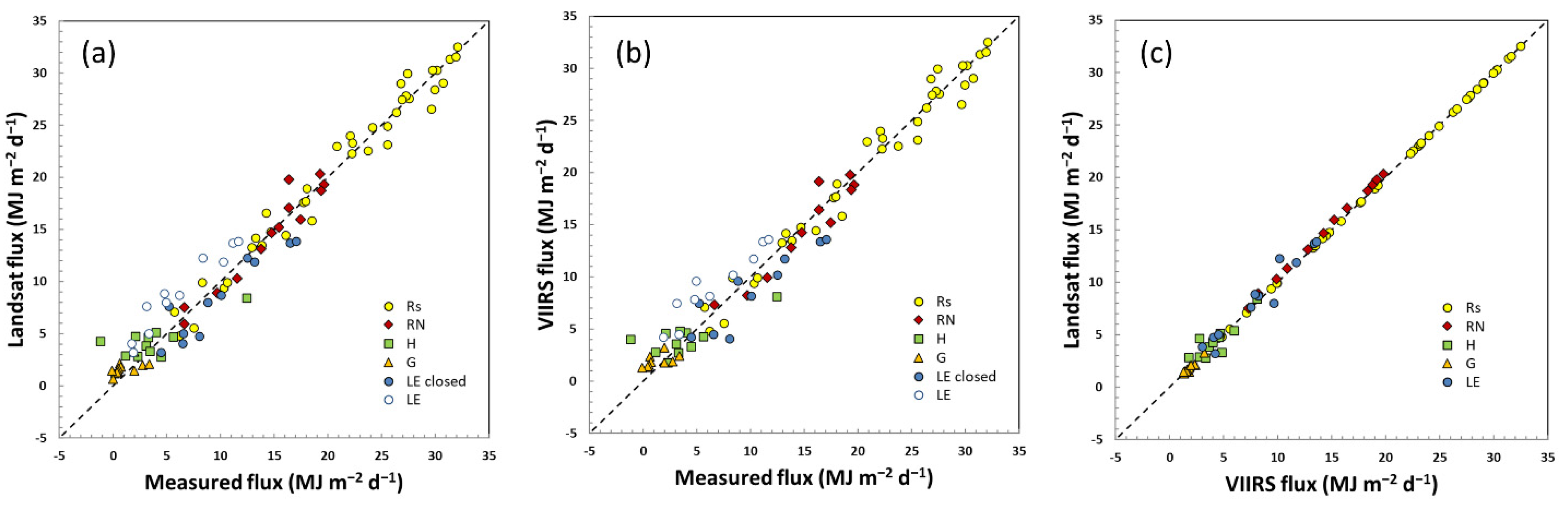
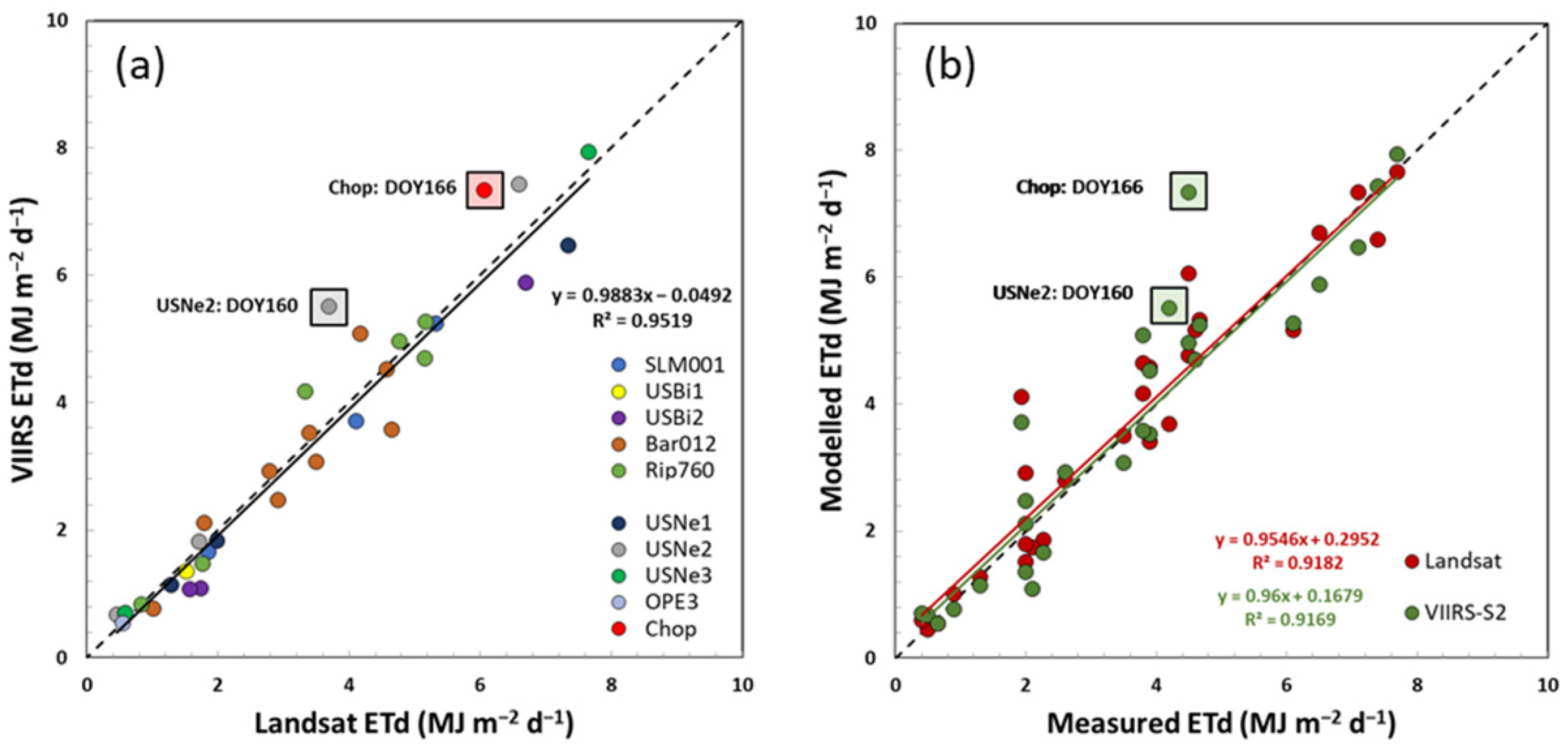
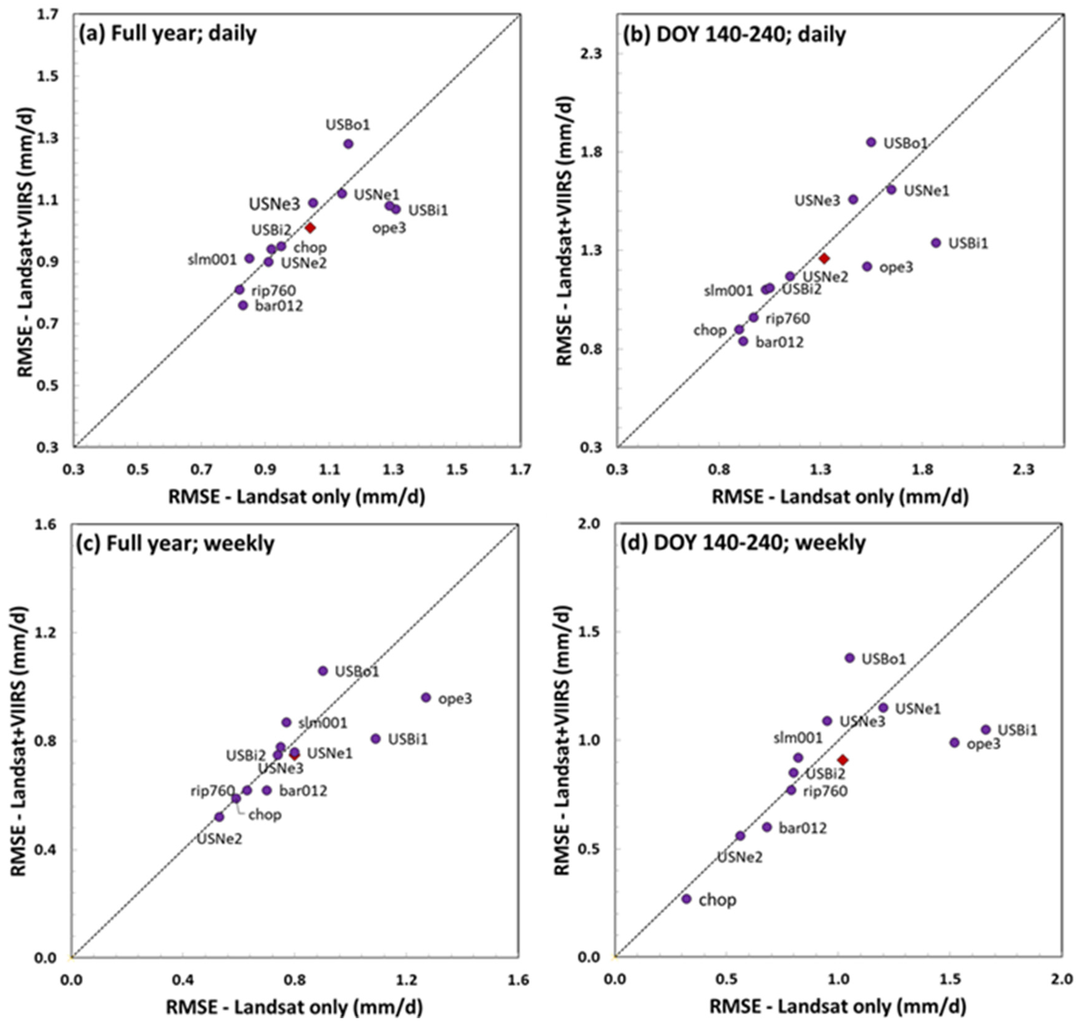
4.1.1. Landsat vs. VIIRS-Landsat ET on Landsat Days

To evaluate consistency of VIIRS 30 m ET with Landsat-based retrievals, modeled daytime-integrated surface fluxes derived from both DisALEXI-Landsat and DisALEXI-VIIRS (using Landsat SR data) on Landsat overpass days were compared with flux tower observations over the USBi2 site in Figure 3a,b and with each other in Figure 3c. Other sites present similar results (not shown).
As seen in Figure 3a,b, both Landsat and VIIRS-derived fluxes agree well with measured ET, with points falling along the one-to-one line indicating reasonable energy budget partitioning. Insolation (Rs) from CFSR and modeled net radiation (Rn), the major energy source driving ET, are comparable with local measurements. Modeled latent heat fluxes (LE) are compared to tower measurements with and without closure correction, with a notably better agreement achieved with the closed results. As shown in Figure 3c, the close alignment of the turbulent fluxes indicates a strong agreement in model agreement using both VIIRS and Landsat TIR inputs.
Mean absolute errors (MAEs) and root mean square errors (RMSEs) between modeled and observed ET (applying energy closure correction as discussed in Section 3.1) over the three sites in the Sierra Loma domain are compared between VIIRS and Landsat, as shown in Figure 4. The two ET data sets show reasonable and comparable accuracy against observations, with MAE (RMSE) ranging from 0.72 (0.79) to 0.84 (1.04) mm d−1 (mean 0.76 (0.89) mm d−1) for Landsat and from 0.71 (0.79) to 0.90 (1.12) mm d−1 (mean 0.81 (0.94) mm d−1) for VIIRS. The somewhat higher RMSE and MAE for VIIRS ET is not unexpected since the native resolution of VIIRS LST (375 m) is coarser than that of Landsat, meaning a larger proportion of subfield structure needs to be reconstructed through sharpening. Furthermore, the LST and VSWIR inputs for DisALEXI-VIIRS modelling are from different platforms with different overpass times and registration errors that may compound the sharpening of VIIRS LST.

4.1.2. Landsat vs. VIIRS-S2 ET on Landsat/S2 Common Days

The accuracy of modeled VIIRS ET estimates generated using S2 VSWIR data was also evaluated against observations and against Landsat ET from same-day acquisitions, as shown in Figure 5 for all tower sites. As with the VIIRS-TIR/Landsat-VSWIR ET retrievals (Figure 3), VIIRS-TIR/S2-VSWIR ET agrees well with direct Landsat retrievals of ET, with a MAE (RMSE) 0.37 (0.48) mm d−1 (Figure 5a). In addition, the modeled Landsat and VIIRS-S2 ET both show good comparison with measured ET (Figure 5b) with a MAE (RMSE) 0.45 (0.64) mm d−1 for Landsat and 0.49 (0.63) mm d−1 for VIIRS-S2, respectively. ET on DOY 166 at the Choptank site and DOY 160 at USNe2, highlighted with boxes in Figure 5, show relatively high discrepancies with the one-to-one line due to cloud contamination in VIIRS LST near the tower site, which was not successfully flagged by VIIRS cloud mask. More discussion of these two days, and ramifications for cloud masking, will be provided in Section 4.3.3.1.
In addition to the evaluation over flux tower sites, the agreement in spatial patterns of ET between same-day VIIRS and Landsat retrievals was also assessed, as highlighted with two examples over the Sierra Loma site (DOY 200) and the Ripperdan site (DOY 177) shown in Figure 6. In general, the ET patterns are similar from the two thermal datasources. In some cases, such as in the Sierra Loma example in Figure 6, VIIRS shows less spatial contrast than Landsat ET with slightly lower values over high-ET patches (e.g., irrigated vineyards) and higher ET over the rainfed grassland/bare soil parts of the scene. This may be related to lower spatial resolution of VIIRS LST with a lower range compared to Landsat; while thermal sharpening can improve the spatial contrast in VIIRS LST, it may not fully reconstruct the underlying structure. The modified thermal sharpening approach used with VIIRS can better account for the misregistration between VIIRS LST and S2 SR, but relative to the standard sharpening it may lead to a loss of spatial details in the sharpened LST and thus ET. In the case of Sierra Loma, this resolution effect may be counterbalanced by the later (afternoon) overpass of VIIRS compared to Landsat, which may accentuate temperature variation over landscapes with differential moisture stress patterns.

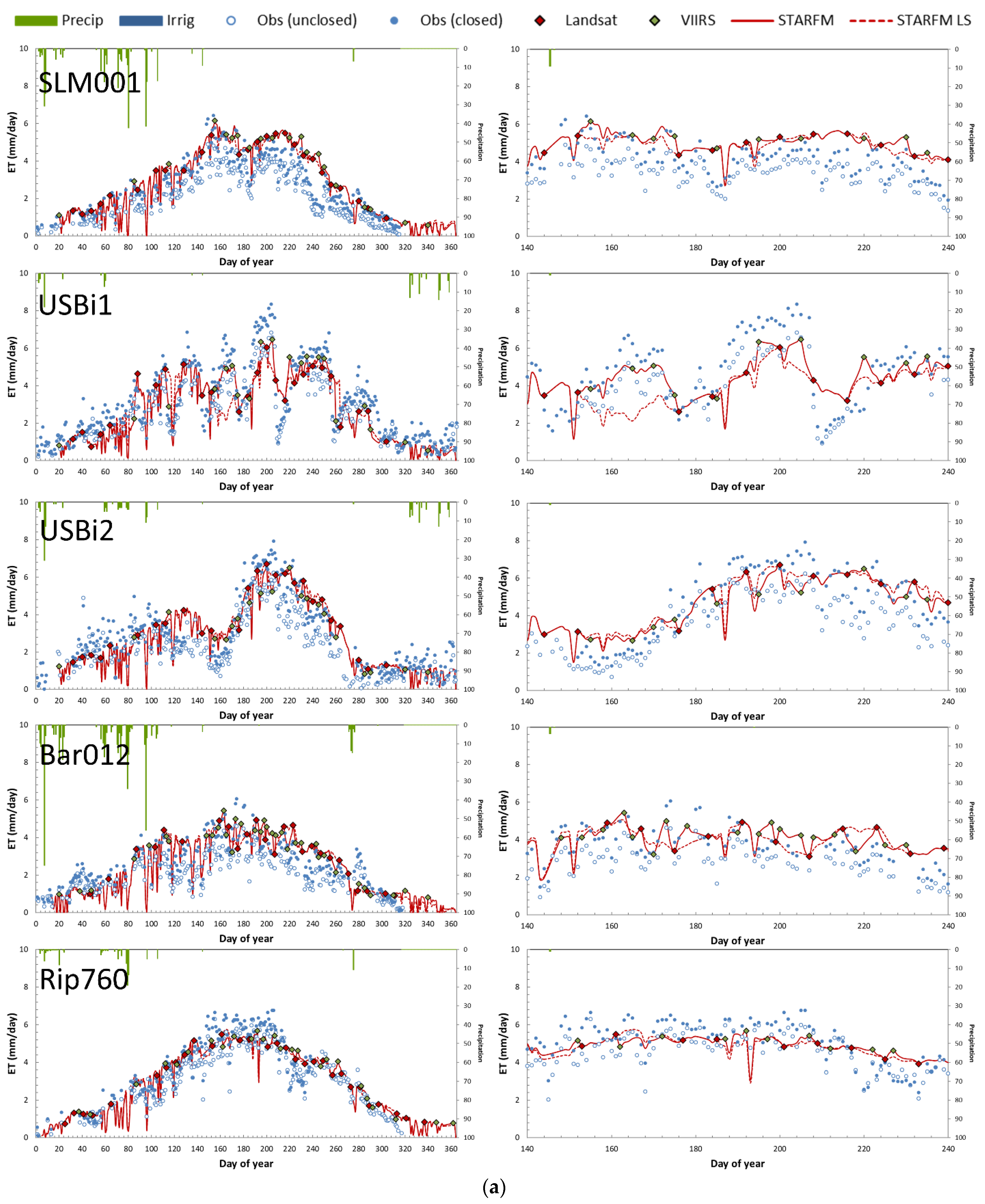
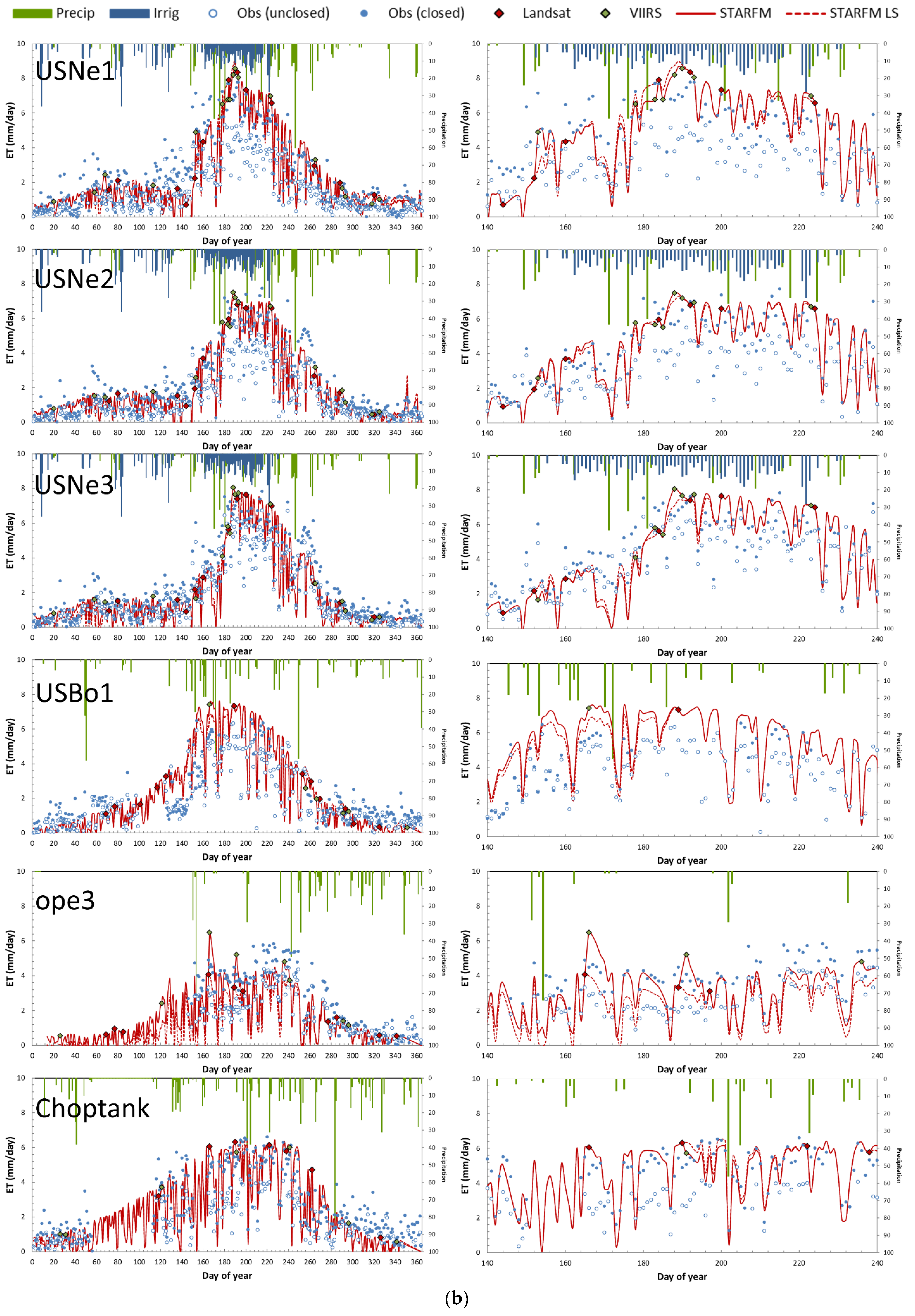
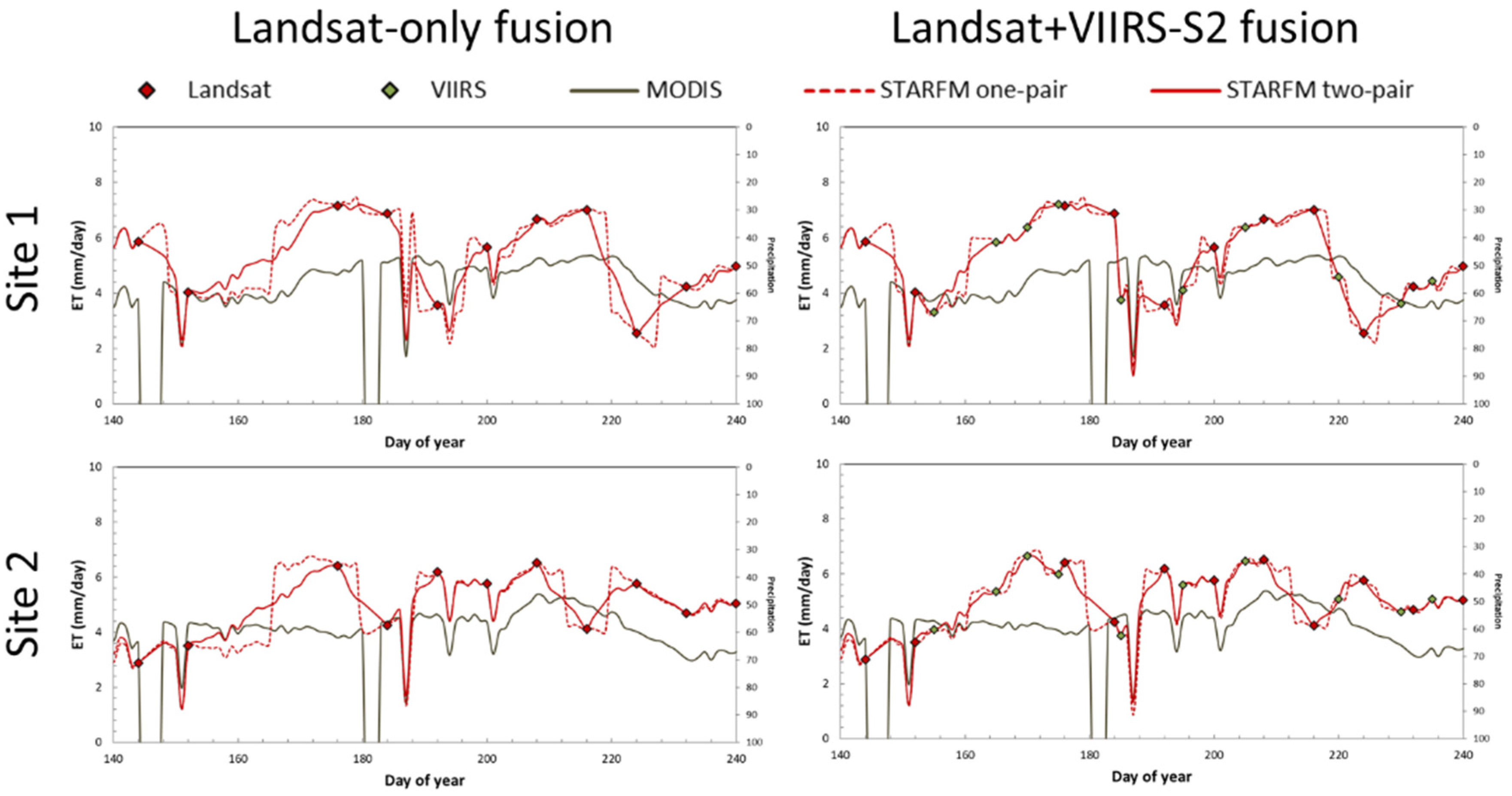
4.2. Evaluation of Fused Daily 30 m ET Time Series

The comparable quality of VIIRS and Landsat ET retrievals at 30 m resolution, as demonstrated in Section 4.1, provides incentive for using these multiple thermal sources as interleaved layers in ET datacube construction. To test the value added by the increased temporal sampling provided by the VIIRS ET layers, we constructed two types of datacubes over the seven domains for year 2018 by fusing 500 m daily MODIS ET with Landsat ET (Landsat-only fusion) and with Landsat and VIIRS ET (Landsat + VIIRS-S2 fusion), as described in Section 2.3.
The modeled 30 m daily ET time series from both Landsat-only and Landsat + VIIRS-S2 fusion over all the tower sites for year 2018 along with direct ET retrievals on Landsat and VIIRS-S2 overpass dates used in fusion are shown in Figure 7. The observational ET time series from flux towers (with and without energy closure correction) are also illustrated. The daily ET time series from the two fusion scenarios show good temporal agreement with each other and are broadly consistent with the observations in trend. At many sites, the Landsat + VIIRS-S2 fusion provides better definition of the ET temporal dynamics than does Landsat-only fusion. In particular, at the USBi1 alfalfa site the four additional VIIRS-S2 samples during DOY 150–180 help to better capture peaks in ET between monthly harvests, which are missed in Landsat-only fusion. Improvements in temporal sampling and sources of inconsistency between Landsat and VIIRS-S2 ET are detailed in the following sections.
Performance of Landsat + VIIRS-S2 vs. Landsat-only ET fusion was quantified using RMSE and mean bias error (MBE) between the fused and observed daily ET time series at both daily and weekly time scales (Table 2), and periods including the full year and the peak growing season. For all sites combined over the full year of 2018, RMSE (MBE) improved slightly by including VIIRS in the fusion, from 1.04 (−0.16) to 1.01 (−0.12) mm d−1 at daily timesteps and from 0.80 (−0.16) to 0.75 (−0.12) mm d−1 at weekly scale.
A few sites show increased RMSE with VIIRS samples included, resulting from poor VIIRS ET retrievals on some days. For instance, the overestimation in VIIRS ET on DOY 166 at the USBo1 site (Figure 7b) resulting from unmasked clouds in the VIIRS TIR imagery served to disimprove the performance of fused daily ET time series. Removing this scene, the RMSE (MBE) at USBo1 decreases from 1.28 (0.17) to 1.16 (0.08) mm d−1 with the remaining VIIRS data layers (see Section 4.3.3.1 for details).
At many of the California sites, there were sufficient clear-sky Landsat overpasses for the Landsat-only fusion to capture the observed ET variability (e.g., SLM001 and Rip760). An exception is the USBi1 alfalfa site, where VIIRS reduced RMSE (MBE) by 18% (13%) and 26% (15%) at daily and weekly timesteps, respectively (Table 2; Figure 8). Performance at the OPE3 soybean site in MD was also improved with the additional VIIRS samples, by 16% (42%) and 24% (32%) at daily and weekly timesteps, respectively. Over the peak growing season (DOY 140–240), the improvement at the two sites was more marked at both daily (28% (59%) for USBi1 and 20% (53%) for OPE3) and weekly (37% (61%) for USBi1 and 35% (44%) for OPE3) timesteps (Table 2; Figure 8). Further discussion of factors impacting the performance at individual sites is provided below.

4.3. Factors Impacting ET Estimates

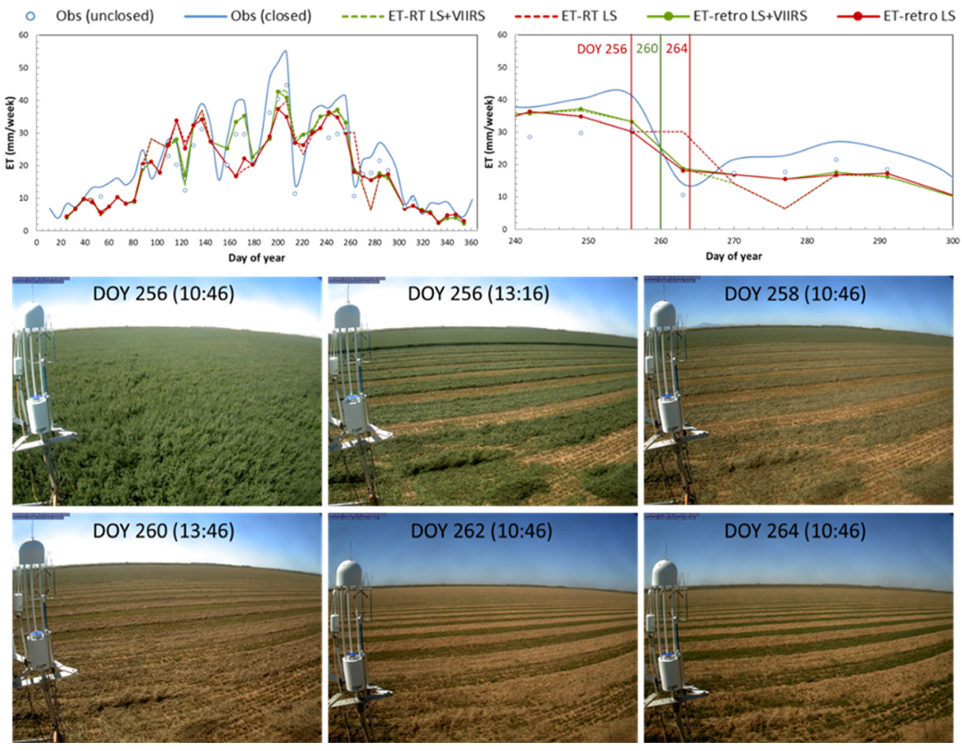
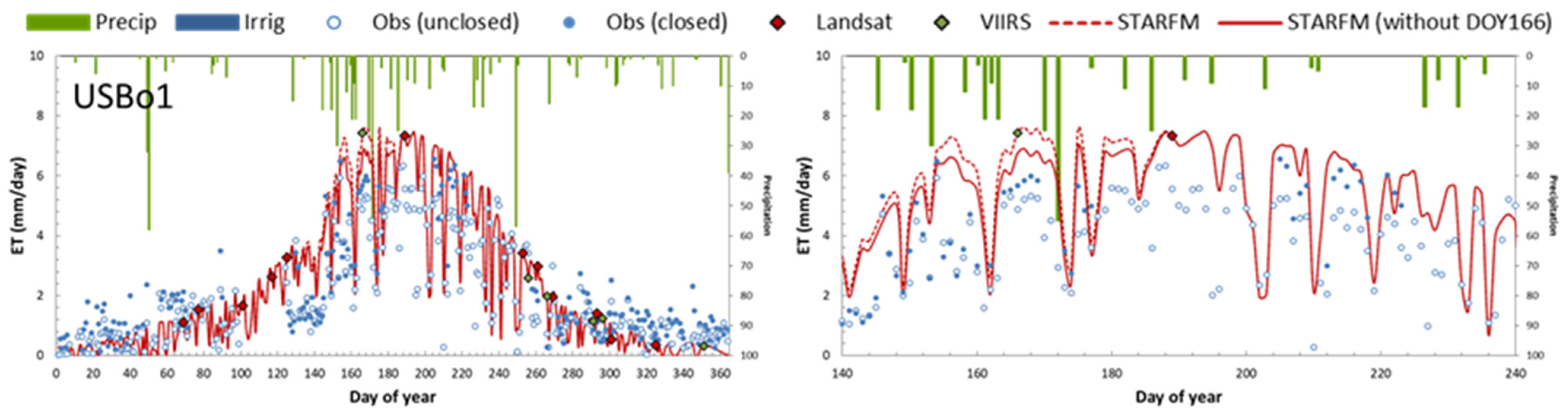
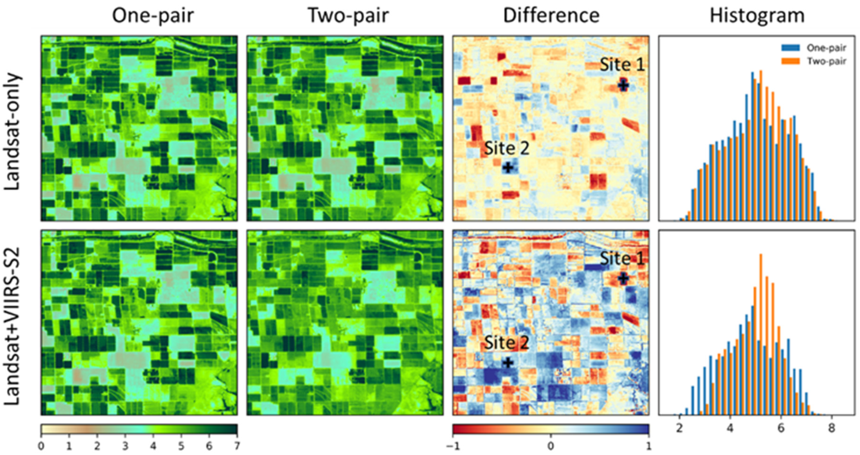
4.3.1. Temporal Sampling

The increased sampling frequency afforded by the additional VIIRS-S2 ET data layers is expected to improve ability to reconstruct daily timeseries using data fusion, particularly at sites with stronger temporal ET dynamics. Including these VIIRS-S2 layers roughly halves the time distance (offset) between a given data fusion prediction date and the closest direct ET retrieval used as the fusion input pair. For all sites, the average pair-prediction time offset over the full year shows a decrease with VIIRS-S2 included (Figure 9a). This decrease is dominated by gains in the non-peak growing season (Figure 9c), while the peak growing season shows smaller decreases in offset (Figure 9b). For both the full year and off season, the mean absolute percent error of fused ETd estimates generally exhibits an increasing trend with respect to offset (Figure 9d,f), highlighting the role of VIIRS-S2 ET in improving the accuracy of ET fusion. As noted above, the two sites that benefited most from the additional VIIRS sampling were the USBi1 site in the Sierra Loma domain and the OPE3 site in the BARC domain. During the peak growing season, including VIIRS-S2 samples leads to a large drop in the maximum offset to below 25 days in the BARC domain. As shown in Figure 9h, the accuracy of fused ETd estimates is similar (MAE ~ 1 mm d−1) for offsets less than 25 days, and starts to degrade for offsets of more than 25 days. While Bondville acquired a VIIRS sample during a long gap during the crop green-up period, reducing the median offset during the peak growing season, cloud contamination on that date caused that additional VIIRS layer to degrade model performance at that site.
The fusion results in Figure 7, Figure 8 and Figure 9 were computed retrospectively, using all image pairs available during the year, both before and after each prediction date. We also examine the impact of temporal sampling frequency for real-time applications, where only an image-pair preceding the prediction date is available. For this analysis, we use the USBi1 site as a test case—due the volatility of the ET curve, this site presents a worse-case scenario for forward-only data fusion. Scatter plots of weekly total ET from ET-retro (retrospective) and ET-RT (real-time) for both Landsat-only and Landsat + VIIRS-S2 fusion in comparison with flux tower observations at the USBi1 site are shown in Figure 10. The ET-retro case serves as the baseline for assessment of the added value afforded by VIIRS-S2 samples in real time. For both retrospective and real-time applications, the Landsat + VIIRS-S2 fusion outperforms the Landsat-only fusion, with better performance for each fusion approach in retrospective application.
The timeseries comparison in Figure 11 (top panel) shows some intervals where the real-time and retrospective weekly ET estimates diverge significantly, whereas Landsat + VIIRS-S2 fusion gives similar results in both configurations. For example, in the interval between DOY 260 and 290, Landsat-only takes a large excursion from reality in real-time mode, but corrects to reasonable performance retrospectively after a bounding image on DOY 264 becomes available. A closer examination of PhenoCam photos from the USBi1 tower (middle and bottom panels of Figure 11) indicates that the contrasting performance between the two Landsat-only cases may be attributed to the Landsat scene on DOY 256. This scene was acquired at ~10:30 am, prior to the cutting operation that occurred that day. The forward Landsat-only fusion therefore assumed full cover until the next Landsat overpass on DOY 264. A VIIRS-S2 pair on DOY 260, shortly post-cutting, enabled the Landsat + VIIRS-S2 timeseries to catch the downturn in ET in both modes. Overall, this case demonstrates the increased value of extra VIIRS-S2 temporal sampling in real time, indicating the potential of Landsat + VIIRS-S2 fusion for operational applications.

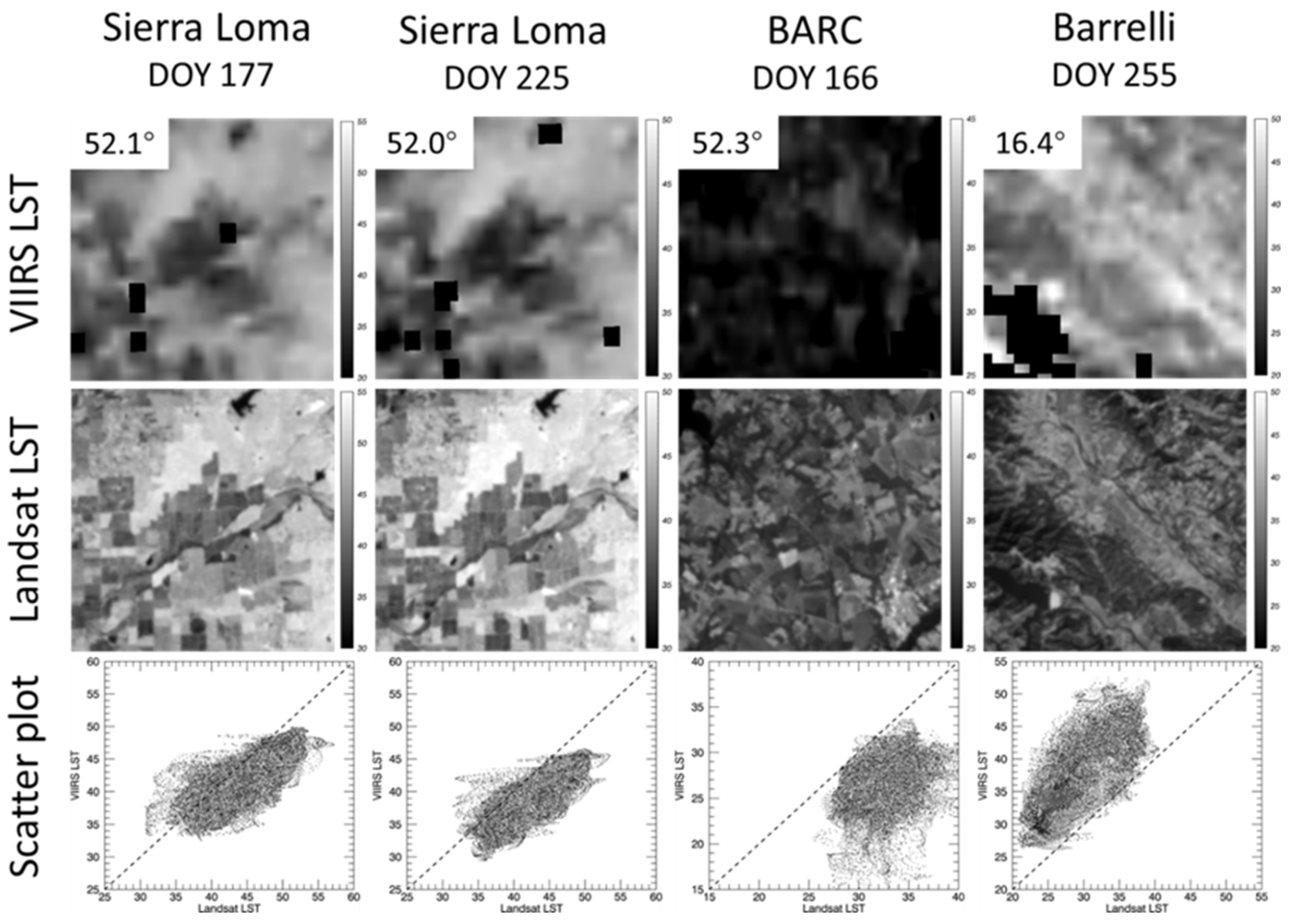
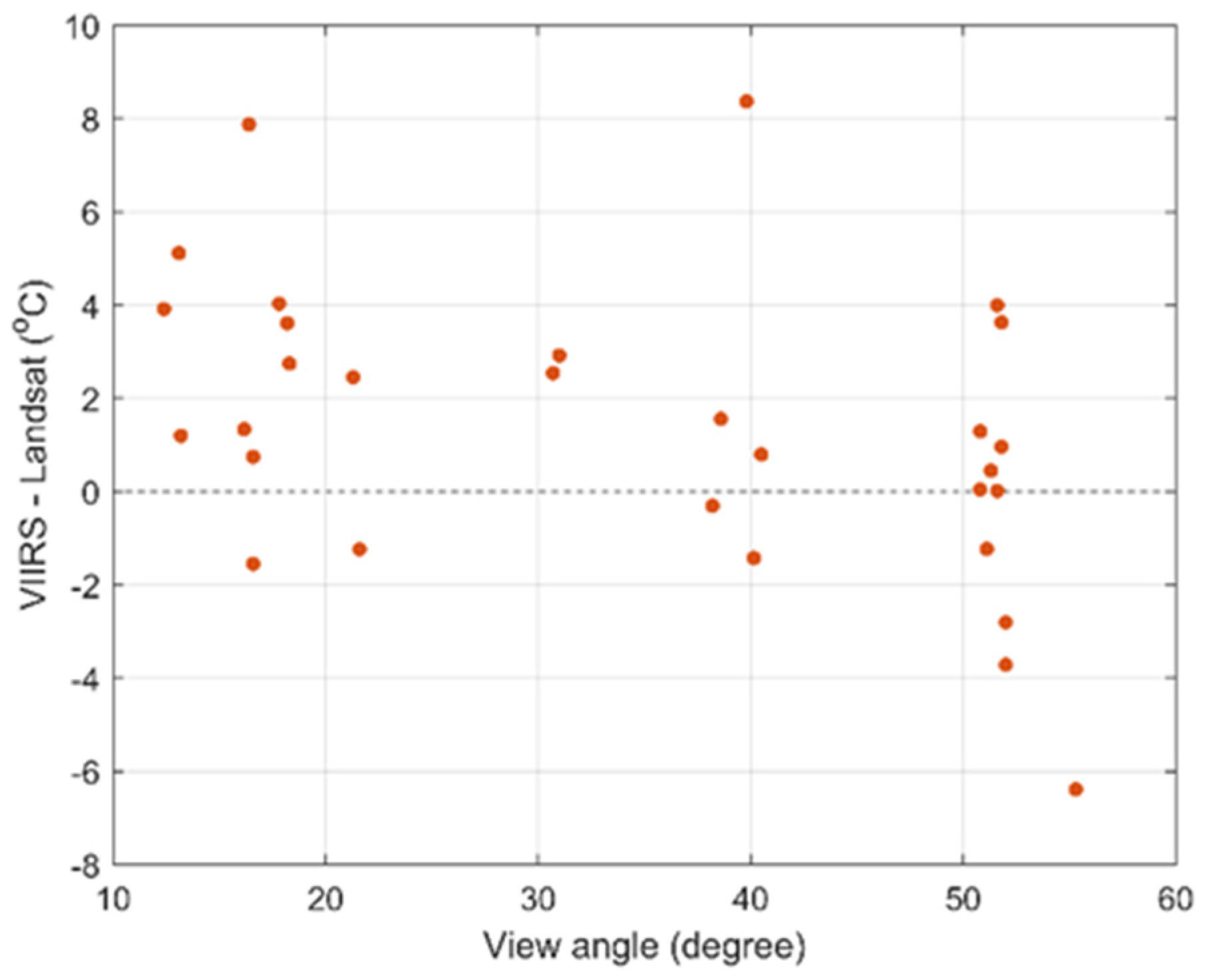
4.3.2. VIIRS View Angle

In a comparison of ECOSTRESS and Landsat 30 m ET retrievals, reference [29] found that accuracy of ECOSTRESS ET estimates degraded with sensor view angle, suggesting a limit of 20° for multi-source fusion. Analysis of VIIRS-S2 ET retrievals also identified a view angle effect. The unique sample aggregation scheme employed in VIIRS, described in Section 3.2.4, results in stepwise resolution degradation as a function of view angle (Figure 12a). To investigate the impact of such pixel resolution degradation on VIIRS ET retrievals, we divided the VIIRS ET into several groups based on view angles in each aggregation zone and then calculated the relative error of ET compared to observations for each group (Figure 12b). The error shows a stepwise upward trend as a function of the view angle, broadly consistent with the change of pixel size change shown in Figure 12a. The result suggests that the loss of spatial detail due to spatial resolution degradation leads to errors in the sharpened LST and thus ET retrievals, though the thermal sharpening helps to increase the spatial consistency between the LSTs at all view angles. It is worth noting that the results reported here are based on limited VIIRS data; more studies are needed to obtain a more robust understanding of the accuracy degradation with view angle.
In addition to degradation of spatial resolution in VIIRS LST at large view angle, there are also cases where thermal radiance magnitude appears to be impacted at view angles approaching the 52° aggregation threshold. The impact of high view angles on LST retrievals was identified at sites where same-day Landsat and VIIRS-S2 overpasses were available. Figure 13 shows four representative cases, comparing VIIRS and Landsat LST at their native resolution on the same day. Absent intervening rainfall or weather front passage, we would generally expect clear-sky LST at the VIIRS acquisition time (~1:30 pm) and low view zenith angle to be higher than at Landsat overpass (~10:30 am), as seen in DOY 255 over Barrelli domain (last column of Figure 13) with a VIIRS view angle of 16.4°. For the high angle cases in Figure 13 (first 3 columns), VIIRS LST is 5–6 °C lower than Landsat LST, although the air temperature measured at the tower was 2–5 °C higher at the VIIRS overpass time. While a partially vegetated surface may appear cooler at higher off-nadir view angles due to larger contributions of Tc to TRAD (Equation (1)) [39], in these cases, VIIRS temperatures are generally lower than Landsat over the full range in cover fraction represented in the scene, indicating a systematic bias.
Expanding this comparison to 30 pairs of same-day Landsat and VIIRS-S2 LST, it was found that VIIRS LST was generally higher than Landsat except for a few cases, especially those with view angle higher than 50° (Figure 14). Statistical tests for two groups of LST pairs based on view angle found that VIIRS LST tends to be significantly higher (p < 0.01) than Landsat LST for all scenes with view angles lower than 40°, consistent with the impact of diurnal cycle on LST. However, for VIIRS LST at view angles larger than 50° this is not the case, suggesting a systematic underestimation of VIIRS LST as shown in Figure 13. This analysis should be revisited with a larger sample of VIIRS-Landsat LST pairs.
These examples demonstrate the potentially undermining impact of high sensor view angles on the quality of VIIRS LST [92,93,94,95] and ET retrievals. While the TSEB model does consider view angle in the partitioning of LST into soil and canopy temperatures (Equation (1)), the magnitude of variability in VIIRS LST with view angle exceeds that expected from directional fractional mixture of component temperatures. Imposing a maximum 50° VIIRS view angle limitation for ET retrievals was beneficial to timeseries comparisons with flux tower observations, particularly at the OPE3 site (Figure 7b) serving to remove the spike around DOY 166.

4.3.3. Cloud Masks

Other discrepancies between Landsat and VIIRS-S2 ET retrievals (e.g., Figure 5) were found to be related to incomplete cloud detection—both in the VIIRS LST and S2 VSWIR products.

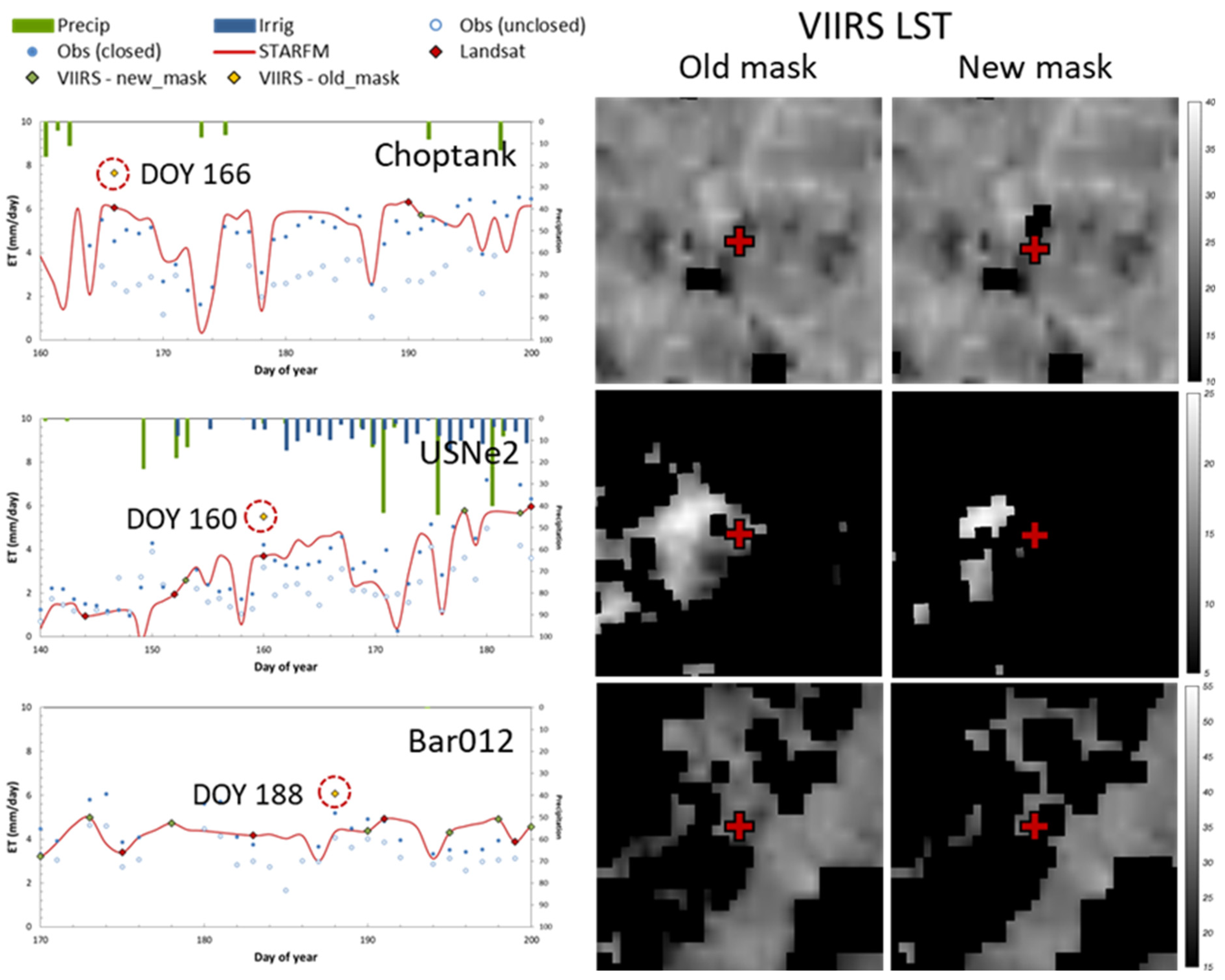
4.3.3.1. VIIRS Cloud Mask

Two VIIRS cloud masks were tested. The original cloud mask was associated with the fire product (375 m I-band) [87,91] which is based on the cloud classification scheme built on the MODIS fire product [96]. Examination of model output showing discrepant ET estimates, both in comparison with tower fluxes and Landsat retrievals, identified several scenes with obvious cloud contaminations in the LST inputs that were not captured in the fire product cloud mask. An additional cloud screening technique was developed by calculating a pixel-based baseline climatology based on the entire VIIRS LST data from year 2013 to 2019. Then, an anomaly is calculated for each pixel, and the pixel is assumed to be cloud contaminated when the anomaly is less than −2.5 standard deviations. This screening is applied with the current cloud mask. The new cloud screening method (named as new mask hereafter) was more effective in flagging cloud-impacted ET retrievals, which tend to be biased high with respect to Landsat retrievals and ET measurements. Examples at the Choptank, Mead, and Barrelli sites are shown in Figure 15. For instance, the VIIRS ET retrieval on DOY 160 at the USNe2 site (5.5 mm d−1) is higher than both Landsat ET (3.7 mm d−1) and the observed flux (4.2 mm d−1). As shown in the second and third columns of Figure 15, the cloud-contaminated pixels near the tower with lower LST were missed by the old mask but successfully flagged by the new mask. A robust cloud mask can improve the fusion accuracy by removing more low-quality VIIRS ET retrievals.

4.3.3.2. HLS (S30) Cloud Mask

Cloud cover in the S2 SR data product, collected at a different acquisition time from VIIRS LST, can also impact the accuracy of the modeled VIIRS ET by contaminating (1) the thermal sharpening of VIIRS LST, and (2) the LAI and albedo inputs to the energy balance model. We demonstrate this impact with an example from the USBo1 flux site in Figure 16 and Figure 17. On DOY 166, a NIR-Red-Green composite of the S2 data (Figure 16a) reveals a cluster of clouds and cloud shadows to the south of the tower site. While the HLS cloud mask successfully detected the bulk of the clouds, the shadows were largely undetected including one compact shadow directly over the tower location. The inaccurate masking propagated the cloud shadow features, which are not observed in the native resolution VIIRS LST (Figure 16c), into the sharpened LST decreasing local temperature by approximately 1–3 K relative to the unsharpened image and leading to an overestimate of ET at the tower site (Figure 17). While this was the only direct ET retrieval in the first half of the peak growing season, between DOY 130 and 180, removal of this scene improved peak season RMSE by 16%.
These examples identify cloud masking in both TIR and VSWIR inputs as a key source of noise in ET timeseries reconstructions.

5. Discussion

Simultaneous TIR/VSWIR acquisitions from the same platform represent the best-case scenario for ET estimation due to inherent advantages over multi-source TIR/VSWIR retrievals. As detailed in [29], simultaneous acquisition can ensure input consistency between LST and vegetation indices for ET models, maximize scene coverage, avoid image misalignments due to sensor registration difference and allow improved cloud detection. In this study, efforts have been taken to reduce the inconsistency between VIIRS LST and S2 SR data. For instance, misregistration errors and variation of pixel footprints between VIIRS LST and S2 SR was partially accounted for in the sharpening process with the modified DMS approach [34]. As reported in Section 4.1, the modelled ET based on the combination of VIIRS LST and S2 SR can achieve a comparable accuracy to Landsat-based retrievals, highlighting the utility of VIIRS-S2 data in ET estimates.
To provide guidance for effective strategies for VIIRS-S2 usage, we further discussed several potential limits in applying VIIRS LST and S2 SR data as inputs for sub-field ET mapping. Unflagged clouds in both VIIRS and S2 bands due to faulty cloud masking, as shown in Section 4.3.3 (e.g., DOY 166 at USBo1/Choptank site), can result in large retrieval errors and thus limit the practical utility of ET estimates. The overpass times for VIIRS and S2 are different, so cloud cover at either acquisition time will affect the image coverage, increasing limitations in the data availability. The VIIRS cloud mask associated with the fire product (I-bands) was improved in this study by applying a baseline climatology-based threshold. Future studies may take advantage of the cloud mask associated with M-bands to help flag anomalous pixels. As reported by [30] and discussed in Section 4.3.3.2, the Fmask used in S2 product of HLS v1.4 may generate erroneous results particularly for hazy conditions, thin clouds and cloud edges since there are no thermal bands. The HLS v1.5 version employing Fmask 4.2, an update of Fmask 4.0 [97] has been released since late 2020, as reported by NASA [98]. Future studies will update to the new HLS version.
Decreased accuracy of ET retrievals using ECOSTRESS LST at high view angles was found to be associated with spatial resolution degradation and misregistration errors in the sharpening process [29]. The spatial resolution of VIIRS degrades with view angle in a stepwise manner, also impacting the accuracy of retrieved ET. We also found VIIRS LST data retrieved at high off-nadir view angles (e.g., >52°) in some cases were systematically lower than same-day Landsat retrievals, resulting in anomalously high ET estimates. Directional effects may have a significant influence on the measured LST with a large field of view [93,99]. Angular variations of LST may have several causes [92,95,100]. One is related to the angular anisotropy of surface emissivity associated with different components of the land covers and water status (e.g., soil moisture). In addition, the structured (3D) surface (e.g., canopy) can have a significant impact on the directional effects of LST through the geometry (e.g., sunlit and shaded elements within the canopy) and viewing more vegetation and less soil than from near nadir [101]. Canopy structural impacts on directional temperature are nominally accommodated in the TSEB model structure via Equation (1). Topography that leads to shadow changes with varying solar and viewing directions can also contribute to angular effects. Finally, nonlinear effects of the longer atmospheric path lengths at higher view angles in the radiative transfer process can be another important factor [94]. The simplified single-channel atmospheric compensation method used here does not account for angular path differences, and is a likely source of bias at high view angles. To reduce uncertainties in ET estimations, VIIRS LST at high sensor view angles should be used with caution.
The value added by the VIIRS-S2 ET data layers as a supplement to Landsat was found to be site- and application-specific. The improvement to ET timeseries was found to be most significant at the USBi1 alfalfa site where ET exhibits multiple seasonal peaks due to monthly cutting, and at the OPE3 site where Landsat data availability in the growing season is limited due to frequent cloud cover. The improvement in timeseries developed in retrospective mode was not significant for a few sites (e.g., Rip760) which had a relatively small mean pair-prediction temporal offset (~5 days) over the peak growing season in the Landsat-only case. This finding is consistent with previous studies suggesting that 5 days or lower revisit frequency is necessary for daily ET mapping with reasonable accuracy [20,21]. However, an experiment simulating real-time ET estimate generation further highlighted the added value afforded by VIIRS-S2 for operational applications, and will become more pronounced considering the latency in data delivery [28]. A reduction in data latency and integration of data from multi-satellite platforms provide useful ways to reduce ET errors in operational settings for crop irrigation management.
In general, sharpening of VIIRS I5 TIR band data appears to be an effective and feasible means for supplementing the HLS dataset with thermal data on S2 overpass dates prior to the anticipated launch of the Landsat Surface Temperature Monitoring (LSTM) mission (Sentinel 8) by the European Space Agency. Replacement of Landsat 7 by Landsat 9, scheduled for launch in September 2021, will further improve HLS utility, providing an additional source of single-platform sampling unencumbered by the scan-line corrector gaps associated with Landsat 7. The ECOSTRESS mission has been extended to 2023, collecting thermal data with a nearly 4 day revisit and ~70 m spatial resolution [29]. In combination, these multiple Landsat and Landsat-like ET data sources will improve our capability to capture rapidly changing ET dynamics (e.g., flash drought) at sub-field scales.

6. Conclusions

In this study, we evaluated the value for field-scale ET retrieval added by augmenting the HLS dataset using VIIRS LST sharpened with Sentinel-2 SR data as a 30 m thermal proxy source on Sentinel-2 overpass dates. Values were assessed in improving Landsat-only 30 m daily ET mapping based on the ALEXI + DisALEXI model across a range of crop types in the continental US through validation against Landsat ET baseline and in-site measurements from eleven flux tower sites. Daily ET maps from Landsat and VIIRS-S2 on the common dates showed similar spatial patterns, regardless of the slightly lower spatial contrast and fewer details observed in VIIRS-S2 ET. Evaluation with flux tower measurements shows comparable accuracy between Landsat and VIIRS-S2 ET estimates directly retrieved on the common overpass dates.
For all eleven sites combined, the improvement of fused daily ET timeseries from the fusion of Landsat + VIIRS-S2 over the Landsat-only case is not very significant (3% for daily and 6% for weekly in terms of RMSE). However, large improvement was observed at several individual sites where the temporal trend of ET showed large variation (e.g., 18% in USBi1 site) or clear-sky Landsat data were not available during periods of rapid changes (e.g., 16% in OPE3 site). The fusion error tends to decrease with respect to an increased temporal sampling of ET retrievals for fusion. The accuracy of fused ET in the peak growing season shows a large drop when the offset between input and target dates reaches close to a month, highlighting the value of increased sampling provided by VIIRS-S2 in capturing the large temporal variability of ET associated with rapid phenology change. For real-time ET estimates, the improvement by Landsat + VIIRS-S2 fusion can be more pronounced (27% in terms of R2) than the retrospective simulation (17%) with improved temporal sampling, highlighting the potential of Landsat + VIIRS-S2 fusion in operational applications. The temporal dynamics of weekly ET were better captured with extra VIIRS samples included (e.g., DOY 260 at USBi1 site).
The accuracy of VIIRS-S2 ET retrievals decreased with increasing view angles but in a stepwise manner, resembling the change in spatial resolution degradation of VIIRS LST. In addition, we found cases with large underestimation of VIIRS LST (as large as 6 K) at view angles of approximately 52°, leading to anomalously high ET retrievals, likely related to spatial resolution degradation and misregistration errors in the sharpening process, angular effects in atmospheric correction, and directional temperature variations over partially vegetated surfaces. These results highlight the need of a careful screening before using VIIRS-S2 ET estimated at high view angles for fusion. We also found cases demonstrating the imperfection of cloud masks from both VIIRS and S2 in detecting clouds, leading to large errors in retrieved ET. A new cloud screening technique for VIIRS developed based on the baseline climatology shows improved performance in this study.

Author Contributions

Conceptualization, J.X., M.C.A. and F.G.; methodology, J.X., M.C.A. and F.G.; software, J.X., M.C.A., F.G., Y.Y. (Yun Yang), K.R.K. and Y.Y. (Yang Yang); validation, J.X. and M.C.A.; formal analysis, J.X.; investigation, J.X., M.C.A. and F.G.; data curation, J.X., M.C.A., F.G., C.H., W.P.K., K.R.K. and Y.Y. (Yang Yang); writing—original draft preparation, J.X.; writing—review and editing, J.X., M.C.A., F.G., W.P.K., C.H. and Y.Y. (Yun Yang); supervision, M.C.A. and F.G.; funding acquisition, M.C.A. and F.G. All authors have read and agreed to the published version of the manuscript.

Funding

This work was funded in part by the NASA’s Land Cover and Land Use MuSLI Program (Grant Number: NNH17ZDA001N-LCLUC), the NASA’s Science of TERRA, AQUA, and SUOMI NPP Program (Grant Number: NNH17ZDA001N-TASNPP), and the NASA ECOSTRESS Program. This research was a contribution from the Long-Term Agroecosystem Research (LTAR) network. LTAR is supported by the United States Department of Agriculture. USDA is an equal opportunity provider and employer. Any use of trade, firm, or product names is for descriptive purposes only and does not imply endorsement by the U.S. Government.

Data Availability Statement

Publicly available satellite datasets were used in this study. The Landsat data were downloaded from https://earthexplorer.usgs.gov/, accessed on 6 July 2021. The HLS data are freely accessible via https://hls.gsfc.nasa.gov/, accessed on 6 July 2021. The MODIS and VIIRS data are available at https://search.earthdata.nasa.gov/, accessed on 6 July 2021. The flux tower data from AmeriFlux sites are accessible at https://ameriflux.lbl.gov/, accessed on 6 July 2021. All other data presented in this study are available on request from the corresponding author for research purposes.

Acknowledgments

The authors wish to thank Andy Suyker for providing flux data for the Mead field sites.

Conflicts of Interest

The authors declare no conflict of interest.

Appendix A

STARFM is a flexible fusion algorithm capable of handling one or two input image-pairs as inputs. In principle a two-pair case utilizing more information outperforms a one-pair case. For Landsat-only fusion, superior performance of the two-pair fusion over the one-pair was demonstrated in [53]. Here, we further assessed the performance of the one-pair and two-pair strategies used in both Landsat-only and Landsat + VIIRS-S2 fusion using fields in the Sierra Loma domain as an example (Figure A1). We investigated the differences in daily ET timeseries generated with the one-pair and two-pair fusion approaches extracted from two small vegetated fields (identified in Figure A2) exhibiting highly dynamic ET values. As demonstrated in Figure A1, the daily ET timeseries from the one-pair fusion exhibit discontinuous increases/decreases around DOY 164 and 220—dates of transition between pairs used for prediction. In contrast, the two-pair case shows smoother and more realistic temporal trends during these transition periods. This temporal difference is less significant in Landsat + VIIRS-S2 fusion due to the increased temporal frequency with additional VIIRS-S2 samples included, which is consistent with the results in [53].
Figure A1. The fused 30 m daily ET time series during DOY 140–240 extracted at two vegetated fields (Site 1 and 2; see Figure A2) from the one-pair case (red dashed) and two-pair case (red solid), for both Landsat-only (left column) and Landsat + VIIRS-S2 fusion (right column).
Remotesensing 13 03420 g0a1
Visual inspection revealed that ET estimates based on two-pair STARFM were slightly more uniform. This is demonstrated in Figure A2, a comparison of one-pair and two-pair fused ET on DOY 218 for both Landsat-only and Landsat + VIIRS-S2 fusion over a subset region (9 × 9 km) of Sierra Loma domain. The two-pair case tends to show less contrast in the spatial pattern of ET than the one-pair case, with lower ET in irrigated fields and fallow fields appearing wetter. The histogram plots over the two images further highlight this point: ET from the one-pair case covers a larger range and shows higher frequency in the high/low end of the distribution. The difference between one-pair and two-pair cases for the Landsat + VIIRS-S2 fusion is larger than Landsat-only fusion, probably because a VIIRS image which generally has a lower spatial contrast than Landsat ET was used in the two-pair case of the Landsat + VIIRS-S2 fusion but not in the one-pair case.
Figure A2. The comparison between one-pair (first column) and two-pair (second column) fused ET on DOY 218 for both Landsat-only (upper row) and Landsat + VIIRS-S2 fusion (bottom row). The difference maps (third column) show two-pair minus one-pair ET. The histograms (fourth column) show the frequency distribution of ET values.
Remotesensing 13 03420 g0a2

References

  1. Oki, T.; Kanae, S. Global hydrological cycles and world water resources. Science 2006, 313, 1068–1072. [Google Scholar] [CrossRef] [Green Version]
  2. Gowda, P.H.; Chavez, J.L.; Colaizzi, P.D.; Evett, S.R.; Howell, T.A.; Tolk, J.A. ET mapping for agricultural water management: Present status and challenges. Irrig. Sci. 2008, 26, 223–237. [Google Scholar] [CrossRef] [Green Version]
  3. Kustas, W.; Anderson, M. Advances in thermal infrared remote sensing for land surface modeling. Agric. For. Meteorol. 2009, 149, 2071–2081. [Google Scholar] [CrossRef]
  4. Kalma, J.D.; McVicar, T.R.; McCabe, M.F. Estimating land surface evaporation: A review of methods using remotely sensed surface temperature data. Surv. Geophys. 2008, 29, 421–469. [Google Scholar] [CrossRef]
  5. Allen, R.G.; Pereira, L.S.; Howell, T.A.; Jensen, M.E. Evapotranspiration information reporting: I. Factors governing measurement accuracy. Agric. Water Manag. 2011, 98, 899–920. [Google Scholar] [CrossRef] [Green Version]
  6. Maes, W.; Steppe, K. Estimating evapotranspiration and drought stress with ground-based thermal remote sensing in agriculture: A review. J. Exp. Bot. 2012, 63, 4671–4712. [Google Scholar] [CrossRef] [Green Version]
  7. Glenn, E.P.; Nagler, P.L.; Huete, A.R. Vegetation index methods for estimating evapotranspiration by remote sensing. Surv. Geophys. 2010, 31, 531–555. [Google Scholar] [CrossRef]
  8. Mu, Q.; Zhao, M.; Running, S.W. Improvements to a MODIS global terrestrial evapotranspiration algorithm. Remote Sens. Environ. 2011, 115, 1781–1800. [Google Scholar] [CrossRef]
  9. Bastiaanssen, W.G.; Menenti, M.; Feddes, R.; Holtslag, A. A remote sensing surface energy balance algorithm for land (SEBAL). 1. Formulation. J. Hydrol. 1998, 212, 198–212. [Google Scholar] [CrossRef]
  10. Allen, R.G.; Tasumi, M.; Trezza, R. Satellite-based energy balance for mapping evapotranspiration with internalized calibration (METRIC)—Model. J. Irrig. Drain. Eng. 2007, 133, 380–394. [Google Scholar] [CrossRef]
  11. Senay, G.B. Satellite psychrometric formulation of the Operational Simplified Surface Energy Balance (SSEBop) model for quantifying and mapping evapotranspiration. Appl. Eng. Agric. 2018, 34, 555–566. [Google Scholar] [CrossRef] [Green Version]
  12. Anderson, M.; Norman, J.; Diak, G.; Kustas, W.; Mecikalski, J. A Two-Source Time-Integrated Model for Estimating Surface Fluxes using Thermal Infrared Remote Sensing. Remote Sens. Environ. 1997, 60, 195–216. [Google Scholar] [CrossRef]
  13. Anderson, M.C.; Norman, J.M.; Mecikalski, J.R.; Otkin, J.A.; Kustas, W.P. A climatological study of evapotranspiration and moisture stress across the continental United States based on thermal remote sensing: 1. Model formulation. J. Geophys. Res. Atmos. 2007, 112, D10117. [Google Scholar] [CrossRef]
  14. Norman, J.; Anderson, M.; Kustas, W.; French, A.; Mecikalski, J.; Torn, R.; Diak, G.; Schmugge, T.; Tanner, B. Remote sensing of surface energy fluxes at 101-m pixel resolutions. Water Resour. Res. 2003, 39, 1221. [Google Scholar] [CrossRef] [Green Version]
  15. Anderson, M.C.; Norman, J.; Mecikalski, J.R.; Torn, R.D.; Kustas, W.P.; Basara, J.B. A multiscale remote sensing model for disaggregating regional fluxes to micrometeorological scales. J. Hydrometeorol. 2004, 5, 343–363. [Google Scholar] [CrossRef]
  16. Anderson, M.C.; Kustas, W.P.; Norman, J.M. Upscaling flux observations from local to continental scales using thermal remote sensing. Agron. J. 2007, 99, 240–254. [Google Scholar] [CrossRef] [Green Version]
  17. Singh, R.K.; Senay, G.B. Comparison of four different energy balance models for estimating evapotranspiration in the Midwestern United States. Water 2016, 8, 9. [Google Scholar] [CrossRef] [Green Version]
  18. Zhang, C.; Long, D.; Zhang, Y.; Anderson, M.C.; Kustas, W.P.; Yang, Y. A decadal (2008–2017) daily evapotranspiration data set of 1 km spatial resolution and spatial completeness across the North China Plain using TSEB and data fusion. Remote Sens. Environ. 2021, 262, 112519. [Google Scholar] [CrossRef]
  19. Anderson, M.C.; Allen, R.G.; Morse, A.; Kustas, W.P. Use of Landsat thermal imagery in monitoring evapotranspiration and managing water resources. Remote Sens. Environ. 2012, 122, 50–65. [Google Scholar] [CrossRef]
  20. Alfieri, J.G.; Anderson, M.C.; Kustas, W.P.; Cammalleri, C. Effect of the revisit interval and temporal upscaling methods on the accuracy of remotely sensed evapotranspiration estimates. Hydrol. Earth Syst. Sci. 2017, 21, 83–98. [Google Scholar] [CrossRef] [Green Version]
  21. Guillevic, P.C.; Olioso, A.; Hook, S.J.; Fisher, J.B.; Lagouarde, J.-P.; Vermote, E.F. Impact of the revisit of thermal infrared remote sensing observations on evapotranspiration uncertainty—A sensitivity study using AmeriFlux data. Remote Sens. 2019, 11, 573. [Google Scholar] [CrossRef] [Green Version]
  22. Gao, F.; Masek, J.; Schwaller, M.; Hall, F. On the blending of the Landsat and MODIS surface reflectance: Predicting daily Landsat surface reflectance. IEEE Trans. Geosci. Remote Sens. 2006, 44, 2207–2218. [Google Scholar] [CrossRef]
  23. Cammalleri, C.; Anderson, M.; Gao, F.; Hain, C.; Kustas, W. A data fusion approach for mapping daily evapotranspiration at field scale. Water Resour. Res. 2013, 49, 4672–4686. [Google Scholar] [CrossRef]
  24. Semmens, K.A.; Anderson, M.C.; Kustas, W.P.; Gao, F.; Alfieri, J.G.; McKee, L.; Prueger, J.H.; Hain, C.R.; Cammalleri, C.; Yang, Y. Monitoring daily evapotranspiration over two California vineyards using Landsat 8 in a multi-sensor data fusion approach. Remote Sens. Environ. 2016, 185, 155–170. [Google Scholar] [CrossRef] [Green Version]
  25. Sun, L.; Anderson, M.C.; Gao, F.; Hain, C.; Alfieri, J.G.; Sharifi, A.; McCarty, G.W.; Yang, Y.; Yang, Y.; Kustas, W.P. Investigating water use over the Choptank River Watershed using a multisatellite data fusion approach. Water Resour. Res. 2017, 53, 5298–5319. [Google Scholar] [CrossRef] [Green Version]
  26. Anderson, M.; Gao, F.; Knipper, K.; Hain, C.; Dulaney, W.; Baldocchi, D.; Eichelmann, E.; Hemes, K.; Yang, Y.; Medellin-Azuara, J. Field-scale assessment of land and water use change over the California Delta using remote sensing. Remote Sens. 2018, 10, 889. [Google Scholar] [CrossRef] [Green Version]
  27. Yang, Y.; Anderson, M.; Gao, F.; Hain, C.; Noormets, A.; Sun, G.; Wynne, R.; Thomas, V.; Sun, L. Investigating impacts of drought and disturbance on evapotranspiration over a forested landscape in North Carolina, USA using high spatiotemporal resolution remotely sensed data. Remote Sens. Environ. 2020, 238, 111018. [Google Scholar] [CrossRef]
  28. Knipper, K.R.; Kustas, W.P.; Anderson, M.C.; Alsina, M.M.; Hain, C.R.; Alfieri, J.G.; Prueger, J.H.; Gao, F.; McKee, L.G.; Sanchez, L.A. Using high-spatiotemporal thermal Satellite ET retrievals for operational water use and stress monitoring in a California vineyard. Remote Sens. 2019, 11, 2124. [Google Scholar] [CrossRef] [Green Version]
  29. Anderson, M.C.; Yang, Y.; Xue, J.; Knipper, K.R.; Yang, Y.; Gao, F.; Hain, C.R.; Kustas, W.P.; Cawse-Nicholson, K.; Hulley, G. Interoperability of ECOSTRESS and Landsat for mapping evapotranspiration time series at sub-field scales. Remote Sens. Environ. 2021, 252, 112189. [Google Scholar] [CrossRef]
  30. Claverie, M.; Ju, J.; Masek, J.G.; Dungan, J.L.; Vermote, E.F.; Roger, J.-C.; Skakun, S.V.; Justice, C. The Harmonized Landsat and Sentinel-2 surface reflectance data set. Remote Sens. Environ. 2018, 219, 145–161. [Google Scholar] [CrossRef]
  31. Guzinski, R.; Nieto, H.; Sandholt, I.; Karamitilios, G. Modelling high-resolution actual evapotranspiration through Sentinel-2 and Sentinel-3 data fusion. Remote Sens. 2020, 12, 1433. [Google Scholar] [CrossRef]
  32. Wolfe, R.E.; Lin, G.; Nishihama, M.; Tewari, K.P.; Tilton, J.C.; Isaacman, A.R. Suomi NPP VIIRS prelaunch and on-orbit geometric calibration and characterization. J. Geophys. Res. Atmos. 2013, 118, 11508–11521. [Google Scholar] [CrossRef] [Green Version]
  33. Guillevic, P.C.; Biard, J.C.; Hulley, G.C.; Privette, J.L.; Hook, S.J.; Olioso, A.; Göttsche, F.M.; Radocinski, R.; Román, M.O.; Yu, Y. Validation of Land Surface Temperature products derived from the Visible Infrared Imaging Radiometer Suite (VIIRS) using ground-based and heritage satellite measurements. Remote Sens. Environ. 2014, 154, 19–37. [Google Scholar] [CrossRef]
  34. Xue, J.; Anderson, M.C.; Gao, F.; Hain, C.; Sun, L.; Yang, Y.; Knipper, K.R.; Kustas, W.P.; Torres-Rua, A.; Schull, M. Sharpening ECOSTRESS and VIIRS land surface temperature using harmonized Landsat-Sentinel surface reflectances. Remote Sens. Environ. 2020, 251, 112055. [Google Scholar] [CrossRef] [PubMed]
  35. Gao, F.; Kustas, W.P.; Anderson, M.C. A data mining approach for sharpening thermal Satellite imagery over land. Remote Sens. 2012, 4, 3287–3319. [Google Scholar] [CrossRef] [Green Version]
  36. Norman, J.M.; Kustas, W.P.; Humes, K.S. Source approach for estimating soil and vegetation energy fluxes in observations of directional radiometric surface temperature. Agric. For. Meteorol. 1995, 77, 263–293. [Google Scholar] [CrossRef]
  37. Kustas, W.P.; Norman, J.M. Evaluation of soil and vegetation heat flux predictions using a simple two-source model with radiometric temperatures for partial canopy cover. Agric. For. Meteorol. 1999, 94, 13–29. [Google Scholar] [CrossRef]
  38. Kustas, W.P.; Norman, J.M. A two-source energy balance approach using directional radiometric temperature observations for sparse canopy covered surfaces. Agron. J. 2000, 92, 847–854. [Google Scholar] [CrossRef]
  39. Kustas, W.P.; Norman, J.M. A two-source approach for estimating turbulent fluxes using multiple angle thermal infrared observations. Water Resour. Res. 1997, 33, 1495–1508. [Google Scholar] [CrossRef]
  40. Cammalleri, C.; Anderson, M.; Kustas, W. Upscaling of evapotranspiration fluxes from instantaneous to daytime scales for thermal remote sensing applications. Hydrol. Earth Syst. Sci. 2014, 18, 1885–1894. [Google Scholar] [CrossRef] [Green Version]
  41. Cammalleri, C.; Anderson, M.; Gao, F.; Hain, C.; Kustas, W. Mapping daily evapotranspiration at field scales over rainfed and irrigated agricultural areas using remote sensing data fusion. Agric. For. Meteorol. 2014, 186, 1–11. [Google Scholar] [CrossRef] [Green Version]
  42. Anderson, M.; Neale, C.; Li, F.; Norman, J.; Kustas, W.; Jayanthi, H.; Chavez, J. Upscaling ground observations of vegetation water content, canopy height, and leaf area index during SMEX02 using aircraft and Landsat imagery. Remote Sens. Environ. 2004, 92, 447–464. [Google Scholar] [CrossRef]
  43. Anderson, M.C.; Kustas, W.P.; Norman, J.M.; Hain, C.R.; Mecikalski, J.R.; Schultz, L.; González-Dugo, M.; Cammalleri, C.; d’Urso, G.; Pimstein, A. Mapping Daily Evapotranspiration at field to Continental Scales Using Geostationary and Polar Orbiting Satellite Imagery. Hydrol. Earth Syst. Sci. 2011, 15, 223–239. [Google Scholar] [CrossRef] [Green Version]
  44. Hoedjes, J.; Chehbouni, A.; Jacob, F.; Ezzahar, J.; Boulet, G. Deriving daily evapotranspiration from remotely sensed instantaneous evaporative fraction over olive orchard in semi-arid Morocco. J. Hydrol. 2008, 354, 53–64. [Google Scholar] [CrossRef] [Green Version]
  45. Van Niel, T.G.; McVicar, T.R.; Roderick, M.L.; van Dijk, A.I.; Renzullo, L.J.; Van Gorsel, E. Correcting for systematic error in satellite-derived latent heat flux due to assumptions in temporal scaling: Assessment from flux tower observations. J. Hydrol. 2011, 409, 140–148. [Google Scholar] [CrossRef]
  46. Delogu, E.; Boulet, G.; Olioso, A.; Coudert, B.; Chirouze, J.; Ceschia, E.; Le Dantec, V.; Marloie, O.; Chehbouni, G.; Lagouarde, J.-P. Reconstruction of temporal variations of evapotranspiration using instantaneous estimates at the time of satellite overpass. Hydrol. Earth Syst. Sci. 2012, 16, 2995–3010. [Google Scholar] [CrossRef] [Green Version]
  47. Gao, F.; Hilker, T.; Zhu, X.; Anderson, M.; Masek, J.; Wang, P.; Yang, Y. Fusing Landsat and MODIS data for vegetation monitoring. Ieee Geosci. Remote Sens. Mag. 2015, 3, 47–60. [Google Scholar] [CrossRef]
  48. Busetto, L.; Meroni, M.; Colombo, R. Combining medium and coarse spatial resolution satellite data to improve the estimation of sub-pixel NDVI time series. Remote Sens. Environ. 2008, 112, 118–131. [Google Scholar] [CrossRef]
  49. Jarihani, A.; McVicar, T.; Van Niel, T.; Emelyanova, I.; Callow, J.; Johansen, K. Blending Landsat and MODIS data to generate multispectral indices: A comparison of “Index-then-Blend” and “Blend-then-Index” approaches. Remote Sens. 2014, 6, 9213–9238. [Google Scholar] [CrossRef] [Green Version]
  50. Rao, Y.; Zhu, X.; Chen, J.; Wang, J. An improved method for producing high spatial-resolution NDVI time series datasets with multi-temporal MODIS NDVI data and Landsat TM/ETM+ images. Remote Sens. 2015, 7, 7865–7891. [Google Scholar] [CrossRef] [Green Version]
  51. Yang, Y.; Anderson, M.C.; Gao, F.; Hain, C.R.; Semmens, K.A.; Kustas, W.P.; Noormets, A.; Wynne, R.H.; Thomas, V.A.; Sun, G. Daily Landsat-scale evapotranspiration estimation over a forested landscape in North Carolina, USA, using multi-satellite data fusion. Hydrol. Earth Syst. Sci. 2017, 21, 1017–1037. [Google Scholar] [CrossRef] [Green Version]
  52. Knipper, K.; Kustas, W.; Anderson, M.; Nieto, H.; Alfieri, J.; Prueger, J.; Hain, C.; Gao, F.; McKee, L.; Alsina, M.M. Using high-spatiotemporal thermal satellite ET retrievals to monitor water use over California vineyards of different climate, vine variety and trellis design. Agric. Water Manag. 2020, 241, 106361. [Google Scholar] [CrossRef]
  53. Yang, Y.; Anderson, M.C.; Gao, F.; Hain, C.; Knipper, K.R.; Kang, Y.; Xue, J.; Yang, Y. Improved daily evapotranspiration estimation using remotely sensed data in a data fusion system. USDA-ARS, Hydrology and Remote Sensing Laboratory, 10300 Baltimore Avenue, Beltsville, MD 20705, USA. 2021. manuscript in preparation. [Google Scholar]
  54. Yang, Y.; Anderson, M.C.; Gao, F.; Wardlow, B.; Hain, C.R.; Otkin, J.A.; Alfieri, J.; Yang, Y.; Sun, L.; Dulaney, W. Field-scale mapping of evaporative stress indicators of crop yield: An application over Mead, NE, USA. Remote Sens. Environ. 2018, 210, 387–402. [Google Scholar] [CrossRef]
  55. Kleinman, P.; Spiegal, S.; Rigby, J.; Goslee, S.; Baker, J.; Bestelmeyer, B.; Boughton, R.; Bryant, R.; Cavigelli, M.; Derner, J. Advancing the sustainability of US agriculture through long-term research. J. Environ. Qual. 2018, 47, 1412–1425. [Google Scholar] [CrossRef] [PubMed]
  56. Kustas, W.P.; Anderson, M.C.; Alfieri, J.G.; Knipper, K.; Torres-Rua, A.; Parry, C.K.; Nieto, H.; Agam, N.; White, W.A.; Gao, F. The grape remote sensing atmospheric profile and evapotranspiration experiment. Bull. Am. Meteorol. Soc. 2018, 99, 1791–1812. [Google Scholar] [CrossRef] [Green Version]
  57. Anderson, M.; Diak, G.; Gao, F.; Knipper, K.; Hain, C.; Eichelmann, E.; Hemes, K.S.; Baldocchi, D.; Kustas, W.; Yang, Y. Impact of insolation data source on remote sensing retrievals of evapotranspiration over the California Delta. Remote Sens. 2019, 11, 216. [Google Scholar] [CrossRef] [Green Version]
  58. Knipper, K.R.; Kustas, W.P.; Anderson, M.C.; Alfieri, J.G.; Prueger, J.H.; Hain, C.R.; Gao, F.; Yang, Y.; McKee, L.G.; Nieto, H. Evapotranspiration estimates derived using thermal-based satellite remote sensing and data fusion for irrigation management in California vineyards. Irrig. Sci. 2019, 37, 431–449. [Google Scholar] [CrossRef]
  59. Yang, Y.; Anderson, M.C.; Gao, F.; Johnson, D.M.; Yang, Y.; Sun, L.; Dulaney, W.; Hain, C.R.; Otkin, J.A.; Prueger, J. Phenological corrections to a field-scale, ET-based crop stress indicator: An application to yield forecasting across the US Corn Belt. Remote Sens. Environ. 2021, 257, 112337. [Google Scholar] [CrossRef]
  60. Verma, S.B.; Dobermann, A.; Cassman, K.G.; Walters, D.T.; Knops, J.M.; Arkebauer, T.J.; Suyker, A.E.; Burba, G.G.; Amos, B.; Yang, H. Annual carbon dioxide exchange in irrigated and rainfed maize-based agroecosystems. Agric. For. Meteorol. 2005, 131, 77–96. [Google Scholar] [CrossRef] [Green Version]
  61. Suyker, A.E.; Verma, S.B. Evapotranspiration of irrigated and rainfed maize–soybean cropping systems. Agric. For. Meteorol. 2009, 149, 443–452. [Google Scholar] [CrossRef] [Green Version]
  62. Hatfield, J.; Prueger, J.; Kustas, W. Spatial and temporal variation of energy and carbon fluxes in Central Iowa. Agron. J. 2007, 99, 285–296. [Google Scholar] [CrossRef] [Green Version]
  63. Meyers, T.; Hollinger, S. An assessment of storage terms in the surface energy balance of maize and soybean. Agric. For. Meteorol. 2004, 125, 105–115. [Google Scholar] [CrossRef]
  64. Houborg, R.; Anderson, M.; Daughtry, C.; Kustas, W.P.; Rodell, M. Using leaf chlorophyll to parameterize light-use-efficiency within a thermal-based carbon, water and energy exchange model. Remote Sens. Environ. 2011, 115, 1694–1705. [Google Scholar] [CrossRef]
  65. De Lannoy, G.; Verhoest, N.; Houser, P.; Gish, T.; Meirvenne, M. Spatial and temporal characteristics of soil moisture in an intensively monitored agricultural field (OPE3). J. Hydrol. 2006, 331, 719–730. [Google Scholar] [CrossRef] [Green Version]
  66. De Lannoy, G.; Houser, P.; Verhoest, N.; Pauwels, V.; Gish, T. Upscaling of point scale measurements to field averages at the OPE3 test site. J. Hydrol. 2007, 343, 1–11. [Google Scholar] [CrossRef] [Green Version]
  67. McCarty, G.W.; Hapeman, C.J.; Sadeghi, A.; Graff, C.; Hively, W.; Lang, M.; Fisher, T.; Jordan, T.; Rice, C.; Codling, E.E.; et al. Water quality and conservation practice effects in the Choptank River Watershed. J. Soil Water Conserv. 2008, 63, 461–474. [Google Scholar] [CrossRef] [Green Version]
  68. Twine, T.E.; Kustas, W.P.; Norman, J.M.; Cook, D.R.; Houser, P.R.; Teyers, T.P.; Prueger, J.H.; Starks, P.J.; Wesely, M.L. Correcting eddy-covariance flux underestimates over a grassland. Agric. For. Meteorol. 2000, 103, 279–300. [Google Scholar] [CrossRef] [Green Version]
  69. Wilson, K.; Goldstein, A.; Falge, E.; Aubinet, M.; Baldocchi, D.; Berbigier, P.; Bernhofer, C.; Ceulemans, R.; Dolman, H.; Field, C.; et al. Energy balance closure at FLUXNET sites. Agric. For. Meteorol. 2002, 113, 223–243. [Google Scholar] [CrossRef] [Green Version]
  70. Meyers, T.; Baldocchi, D. Current micrometeorological flux methodologies with applications in agriculture. Micrometeorol. Agric. Syst. 2005, 47, 381–396. [Google Scholar]
  71. Alfieri, J.G.; Kustas, W.P.; Prueger, J.H.; Hipps, L.E.; Evett, S.R.; Basara, J.B.; Neale, C.M.U.; French, A.N.; Colaizzi, P.; Agam, N.; et al. On the discrepancy between eddy covariance and lysimetry-based surface flux measurements under strongly advective conditions. Adv. Water Resour. 2012, 50, 62–78. [Google Scholar] [CrossRef] [Green Version]
  72. Saha, S.; Moorthi, S.; Wu, X.; Wang, J.; Nadiga, S.; Tripp, P.; Behringer, D.; Hou, Y.-T.; Chuang, H.-y.; Iredell, M.; et al. The NCEP Climate Forecast System Version 2. J. Clim. 2014, 27, 2185–2208. [Google Scholar] [CrossRef]
  73. Hansen, M.; Defries, R.; Townshend, J.; Sohlberg, R.A. Global land cover classi cation at 1km spatial resolution using a classification tree approach. Int. J. Remote Sens. 2000, 21, 1331–1364. [Google Scholar] [CrossRef]
  74. Fry, J.; Xian, G.S.; Jin, S.; Dewitz, J.; Homer, C.; Yang, L.; Barnes, C.; Herold, N.; Wickham, J. Completion of the 2006 national land cover database for the conterminous United States. Photogramm. Eng. Remote Sens. 2011, 77, 858–864. [Google Scholar]
  75. Wickham, J.; Stehman, S.; Gass, L.; Dewitz, J.; Fry, J.; Wade, T. Accuracy assessment of NLCD 2006 land cover and impervious surface. Remote Sens. Environ. 2013, 130, 294–304. [Google Scholar] [CrossRef]
  76. Gao, F.; Anderson, M.C.; Kustas, W.P.; Wang, Y. Simple method for retrieving leaf area index from Landsat using MODIS leaf area index products as reference. J. Appl. Remote Sens. 2012, 6, 063554. [Google Scholar]
  77. Liang, S. Narrowband to broadband conversions of land surface albedo I algorithms. Remote Sens. Environ. 2001, 76, 213–238. [Google Scholar] [CrossRef]
  78. Berk, A.; Bernstein, L.S.; Robertson, D.C. Modtran: A Moderate Resolution Model for Lowtran; Spectral Sciences Inc.: Burlington, MA, USA, 1987. [Google Scholar]
  79. Vermote, E.; Justice, C.; Claverie, M.; Franch, B. Preliminary analysis of the performance of the Landsat 8/OLI land surface reflectance product. Remote Sens. Environ. 2016, 185, 46–56. [Google Scholar] [CrossRef] [PubMed]
  80. Zhu, Z.; Wang, S.; Woodcock, C.E. Improvement and expansion of the Fmask algorithm: Cloud, cloud shadow, and snow detection for Landsats 4–7, 8, and Sentinel 2 images. Remote Sens. Environ. 2015, 159, 269–277. [Google Scholar] [CrossRef]
  81. Franch, B.; Vermote, E.; Skakun, S.; Roger, J.-C.; Masek, J.; Ju, J.; Villaescusa-Nadal, J.; Santamaría-Artigas, A. A method for Landsat and Sentinel 2 (HLS) BRDF normalization. Remote Sens. 2019, 11, 632. [Google Scholar] [CrossRef] [Green Version]
  82. Price, J.C. Estimating surface temperatures from satellite thermal infrared data—A simple formulation for the atmospheric effect. Remote Sens. Environ. 1983, 13, 353–361. [Google Scholar] [CrossRef]
  83. Polivka, T.N.; Hyer, E.J.; Wang, J.; Peterson, D.A. First global analysis of saturation artifacts in the VIIRS infrared channels and the effects of sample aggregation. Ieee Geosci. Remote Sens. Lett. 2015, 12, 1262–1266. [Google Scholar] [CrossRef]
  84. Tilton, J.C.; Lin, G.; Tan, B. Measurement of the band-to-band registration of the SNPP VIIRS imaging system from on-orbit data. IEEE J. Sel. Top. Appl. Earth Obs. Remote Sens. 2017, 10, 1056–1067. [Google Scholar] [CrossRef] [PubMed] [Green Version]
  85. Schueler, C.; Lee, T.; Miller, S. VIIRS constant spatial-resolution advantages. Int. J. Remote Sens. 2013, 34, 5761–5777. [Google Scholar] [CrossRef]
  86. Gladkova, I.; Ignatov, A.; Shahriar, F.; Kihai, Y.; Hillger, D.; Petrenko, B. Improved VIIRS and MODIS SST imagery. Remote Sens. 2016, 8, 79. [Google Scholar] [CrossRef] [Green Version]
  87. Schroeder, W.; Oliva, P.; Giglio, L.; Csiszar, I.A. The New VIIRS 375 m active fire detection data product: Algorithm description and initial assessment. Remote Sens. Environ. 2014, 143, 85–96. [Google Scholar] [CrossRef]
  88. Anderson, M.C.; Kustas, W.P.; Alfieri, J.G.; Gao, F.; Hain, C.; Prueger, J.H.; Evett, S.; Colaizzi, P.; Howell, T.; Chávez, J.L. Mapping daily evapotranspiration at Landsat spatial scales during the BEAREX’08 field campaign. Adv. Water Resour. 2012, 50, 162–177. [Google Scholar] [CrossRef] [Green Version]
  89. Li, F.; Kustas, W.P.; Anderson, M.C.; Prueger, J.H.; Scott, R.L. Effect of remote sensing spatial resolution on interpreting tower-based flux observations. Remote Sens. Environ. 2008, 112, 337–349. [Google Scholar] [CrossRef]
  90. European Space Agency. Sentinel-2 User Handbook. ESA Standard Document Paris, France 2015. 2015. Available online: https://sentinel.esa.int/documents/247904/685211/Sentinel-2_User_Handbook (accessed on 25 January 2021).
  91. Schroeder, W.; Giglio, L. Visible Infrared Imaging Radiometer Suite (VIIRS) 375 m Active Fire Detection and Charaterization Algorithm Theoretical Basis Document 1.0. NASA 2016. Available online: https://viirsland.gsfc.nasa.gov/PDF/VIIRS_activefire_375m_ATBD.pdf (accessed on 10 April 2020).
  92. Li, Z.-L.; Tang, B.-H.; Wu, H.; Ren, H.; Yan, G.; Wan, Z.; Trigo, I.F.; Sobrino, J.A. Satellite-derived land surface temperature: Current status and perspectives. Remote Sens. Environ. 2013, 131, 14–37. [Google Scholar] [CrossRef] [Green Version]
  93. Ren, H.; Liu, R.; Yan, G.; Mu, X.; Li, Z.-L.; Nerry, F.; Liu, Q. Angular normalization of land surface temperature and emissivity using multiangular middle and thermal infrared data. IEEE Trans. Geosci. Remote Sens. 2014, 52, 4913–4931. [Google Scholar]
  94. Hulley, G.C.; Hughes, C.G.; Hook, S.J. Quantifying uncertainties in land surface temperature and emissivity retrievals from ASTER and MODIS thermal infrared data. J. Geophys. Res. Atmos. 2012, 117, D23113. [Google Scholar] [CrossRef] [Green Version]
  95. Cao, B.; Liu, Q.; Du, Y.; Roujean, J.-L.; Gastellu-Etchegorry, J.-P.; Trigo, I.F.; Zhan, W.; Yu, Y.; Cheng, J.; Jacob, F. A review of earth surface thermal radiation directionality observing and modeling: Historical development, current status and perspectives. Remote Sens. Environ. 2019, 232, 111304. [Google Scholar] [CrossRef]
  96. Giglio, L.; Schroeder, W.; Justice, C.O. The collection 6 MODIS active fire detection algorithm and fire products. Remote Sens. Environ. 2016, 178, 31–41. [Google Scholar] [CrossRef] [PubMed] [Green Version]
  97. Qiu, S.; Zhu, Z.; He, B. Fmask 4.0: Improved cloud and cloud shadow detection in Landsats 4–8 and Sentinel-2 imagery. Remote Sens. Environ. 2019, 231, 111205. [Google Scholar] [CrossRef]
  98. Masek, J.G. Harmonized landsat Sentinel-2 (HLS) Product User’s Guide—Product Version 1.5; National Aeronautics and Space Administration (NASA): Washington, DC, USA, 2020. [Google Scholar]
  99. Wang, D.; Chen, Y.; Hu, L.; Voogt, J.A.; Gastellu-Etchegorry, J.-P.; Krayenhoff, E.S. Modeling the angular effect of MODIS LST in urban areas: A case study of Toulouse, France. Remote Sens. Environ. 2021, 257, 112361. [Google Scholar] [CrossRef]
  100. Liu, X.; Tang, B.-H.; Wu, H.; Tang, R.; Li, Z.-L.; Shang, G. A method for angular normalization of land surface temperature products based on component temperatures and fractional vegetation cover. In Proceedings of the IEEE International Geoscience and Remote Sensing Symposium (IGARSS), Yokohama, Japan, 28 July–2 August 2019; pp. 1849–1852. [Google Scholar]
  101. Chehbouni, A.; Nouvellon, Y.; Kerr, Y.; Moran, M.S.; Watts, C.; Prevot, L.; Goodrich, D.; Rambal, S. Directional effect on radiative surface temperature measurements over a semiarid grassland site. Remote Sens. Environ. 2001, 76, 360–372. [Google Scholar] [CrossRef]
Figure 1. Schematic diagram representing the flow of multi-source ET processing and data fusion system. The schematic is adapted from Figure 2 in [29].
Remotesensing 13 03420 g001
Figure 2. Study area covering the U.S. The ET maps show subregions (300 × 300 30 m pixels) of the seven study area domains, with flux tower sites indicated with white crosses.
Remotesensing 13 03420 g002
Figure 3. Scatterplots of Landsat/VIIRS-retrieved and observed daytime-integrated fluxes on Landsat overpass dates at USBi2 site. Comparisons between (a) Landsat and observations, (b) VIIRS (using Landsat SR) and observations, and (c) Landsat and VIIRS. Rs: solar radiation; Rn: net radiation; H: sensible heat flux; G: soil heat flux; LE: latent heat flux, where ‘closed’ indicates energy balance closure. Rs is derived from CFSR data, so it is the same for Landsat and VIIRS.
Remotesensing 13 03420 g003
Figure 4. Comparison of RMSE and MAE in retrieved daily Landsat ET and VIIRS ET against observed ET on Landsat overpass days at SLM001, USBi1 and USBi2 sites.
Remotesensing 13 03420 g004
Figure 5. (a) Comparison of modeled Landsat and VIIRS daily ET on common days of overpass in 2018 at all the flux sites. (b) The same as (a), but between modeled and measured ET. DOY 166 at the Choptank site and DOY 160 at USNe2, highlighted with boxes, were shown for comparison but not used in the linear regression due to cloud contamination in VIIRS LST undetected by the VIIRS cloud mask.
Remotesensing 13 03420 g005
Figure 6. Comparison in spatial pattern of native LST (°C; first column), sharpened LST (°C; second column), and daily ET estimates (mm d−1; third column) between Landsat and VIIRS-S2 on DOY 200 over Sierra Loma domain (top two rows) and DOY 177 over Ripperdan domain (bottom two rows). Daily ET difference maps (VIIRS-S2 minus Landsat) are shown in the fourth column.
Remotesensing 13 03420 g006
Figure 7. (a). Model-measurement time-series intercomparison at the CA flux tower sites for the full year of 2018 (left) and peak growing season (DOY 140–240; right). (b). Model-measurement time-series intercomparison at the MD, IL and NE flux tower sites for the full year of 2018 (left) and peak growing season (DOY 140–240; right).
Remotesensing 13 03420 g007aRemotesensing 13 03420 g007b
Figure 8. Comparison of RMSE in (a,b) daily and (c,d) weekly ET developed with and without VIIRS over (a,c) the full year of 2018 and (b,d) peak growing season (DOY 140–240).
Remotesensing 13 03420 g008
Figure 9. Boxplot of offset (in days) between direct retrieval date and prediction date over each domain for (a) the full year, (b) the peak growing and (c) non-peak growing season. Fusion accuracy in terms of mean absolute percent error (MAE/<O>) as a function of offset days between input and target dates for (d) the full year, (e) the peak growing and (f) non-peak growing season. <O> is the mean of the observed ET. (gi) Same as (d,f), but for MAE (mm d−1). Note that the fusion accuracy plots are from the Landsat-only fusion timeseries.
Remotesensing 13 03420 g009
Figure 10. Scatterplots comparing measured and modeled weekly ET for both Landsat-only (LS) and Landsat + VIIRS-S2 (LS+VIIRS) fusion from the (a) baseline retrospective fusion model (retro) and (b) real-time fusion model (RT) for the USBi1 site.
Remotesensing 13 03420 g010
Figure 11. Top panel, the time series of weekly total ET for Landsat-only (red lines) and Landsat + VIIRS-S2 (green lines) fusion in both retrospective (solid lines) and operational (dashed lines) modeling schemes, in comparison with measured weekly total ET (both closed and unclosed) at the USBi1 tower site in 2018. The vertical lines indicate the overpass dates of Landsat and VIIRS-S2. Middle and bottom panels, photographs from a PhenoCam at USBi1 site showing alfalfa canopy biomass changes on some key days.
Remotesensing 13 03420 g011
Figure 12. (a) The change of the pixel size of VIIRS LST data as a function of scan angles, adopted from VIIRS 375 m Active Fire Detection and Characterization ATBD 1.0 [91]; (b) Mean relative errors of VIIRS daily ET retrievals for different view angle categories.
Remotesensing 13 03420 g012
Figure 13. Comparison of VIIRS (up row) and Landsat LST (middle row) at native resolution on days with different view angles over Sierra Loma, BARC and Barrelli domain (400 × 400 pixels), with corresponding scatter plots of VIIRS and Landsat LST shown in the (bottom row).
Remotesensing 13 03420 g013
Figure 14. Difference in mean LST between VIIRS and Landsat over the 400 × 400 pixel area as a function of view angle on common overpass days over all the domains.
Remotesensing 13 03420 g014
Figure 15. Comparison of ET retrievals at the Choptank, USNe2 and Bar012 sites (first column). VIIRS ET with cloud cover near the tower not successfully flagged by the old cloud mask is highlighted in red circle. Comparison between VIIRS LST maps (400 × 400) with old (second column) and new (third column) cloud mask, centered on each flux tower site. The black pixel indicates cloud cover detected by the mask, and the red cross represents the location of flux tower. Note that DOY 166 at Choptank site and DOY 160 at USNe2 site are the two points highlighted in Figure 5.
Remotesensing 13 03420 g015
Figure 16. (a) The NIR-Red-Green composite (400 × 400) of S2 SR bands, (b) the sharpened VIIRS LST and (c) native VIIRS LST on DOY 166 centered on the USBo1 site over Bondville domain. The zoom-in view (50 × 50) of (ac) is shown in the bottom row. Yellow cross represents the location of flux tower.
Remotesensing 13 03420 g016
Figure 17. Comparison in the modeled ET time-series between with (dashed red line) and without (solid red line) DOY 166 at the USBo1 tower site of Bondville domain for the full year of 2018 (left) and peak growing season (DOY 140–240; right).
Remotesensing 13 03420 g017
Table 1. Characteristics of satellite sensors used in this study.
Platform/SensorLaunch DateEquatorial
Crossing Time
Spatial ResolutionTemporal
Resolution
View Zenith Angle
SR BandsTIR Bands
Landsat 715 April 199910:00 a.m.30 m60 m16 day<7.5°
Landsat 811 February 201310:00 a.m.30 m100 m16 day<7.5°
Sentinel-2A23 June 201510:30 a.m.10–20 m-10 day<11.93°
Sentinel-2B7 March 201710:30 a.m.10–20 m-10 day<11.93°
VIIRS (I bands)28 October 20111:30 p.m.375 m375 m~daily<70°
MODIS(Terra) 18 December 199910:30 a.m.250–500 m1000 mA few times per day<65°
(Aqua) 5 May 20021:30 p.m.
Table 2. Statistical metrics of model performance (RMSE and MBE) for estimating ET (mm d−1) at daily and weekly timesteps with Landsat-only (L) and Landsat + VIIRS-S2 (L+V), over the full year of 2018 and the peak growing season (DOY 140–240) by tower and for all towers combined.
Full YearDOY 140–240
TimescaleDomainTowerRMSE LRMSE L + VMBE LMBE L + VRMSE LRMSE L + VMBE LMBE L + V
DailySierra LomaSLM0010.850.910.460.551.031.100.710.85
USBi11.311.07−0.53−0.461.871.34−0.98−0.40
USBi20.920.94−0.08−0.171.051.110.230.01
BarrelliBar0120.830.760.110.100.920.840.360.32
RipperdanRip7600.820.81−0.12−0.120.970.96−0.31−0.27
MeadUSNe11.141.12−0.04−0.081.651.610.030.03
USNe20.910.90−0.21−0.141.151.17−0.060.03
USNe31.051.09−0.36−0.291.461.56−0.14−0.15
BondvilleUSBo11.161.280.120.171.551.851.021.37
BARCOPE31.291.08−0.91−0.531.531.22−1.31−0.61
ChoptankChop0.950.95−0.21−0.210.900.900.210.10
All1.041.01−0.16−0.121.321.26−0.060.07
Weekly All0.800.75−0.16−0.121.020.91−0.080.04
Publisher’s Note: MDPI stays neutral with regard to jurisdictional claims in published maps and institutional affiliations.

