
High-Resolution Terrain Modeling Using Airborne LiDAR Data with Transfer Learning
by
 , ,
, ,
Huxiong Li
1, 
Weiya Ye
2,
Jun Liu
3,
Weikai Tan
2,
Saied Pirasteh
2,4,* ,
,
Sarah Narges Fatholahi
2 and
Jonathan Li
2 1
School of Mechanical and Electrical Engineering, Shaoxin University, Shaoxing 312000, China
2
Department of Geography and Environmental Management, University of Waterloo, Waterloo, ON N2L 3G1, Canada
3
College of Computer Science and Artificial Intelligence, Wenzhou University, Wenzhou 325035, China
4
Faculty of Geosciences & Environmental Engineering, Southwest Jiaotong University, Chengdu 611756, China
*
Author to whom correspondence should be addressed.
Remote Sens. 2021, 13(17), 3448; https://0-doi-org.brum.beds.ac.uk/10.3390/rs13173448
Submission received: 17 July 2021
/
Revised: 22 August 2021
/
Accepted: 27 August 2021
/
Published: 31 August 2021
(This article belongs to the Special Issue 3D Reconstruction Based on Remote Sensing Imagery and Lidar Point Cloud)
Abstract
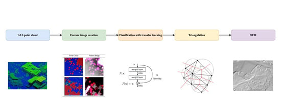
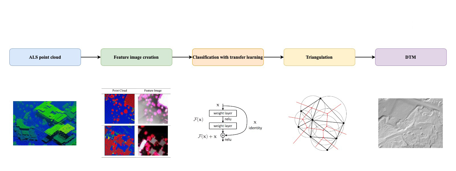
:This study presents a novel workflow for automated Digital Terrain Model (DTM) extraction from Airborne LiDAR point clouds based on a convolutional neural network (CNN), considering a transfer learning approach. The workflow consists of three parts: feature image generation, transfer learning using ResNet, and interpolation. First, each point is transformed into a featured image based on its elevation differences with neighboring points. Then, the feature images are classified into ground and non-ground using ImageNet pretrained ResNet models. The ground points are extracted by remapping each feature image to its corresponding points. Last, the extracted ground points are interpolated to generate a continuous elevation surface. We compared the proposed workflow with two traditional filters, namely the Progressive Morphological Filter (PMF) and the Progressive Triangulated Irregular Network Densification (PTD). Our results show that the proposed workflow establishes an advantageous DTM extraction accuracy with yields of only 0.52%, 4.84%, and 2.43% for Type I, Type II, and the total error, respectively. In comparison, Type I, Type II, and the total error for PMF are 7.82%, 11.60%, and 9.48% and for PTD 1.55%, 5.37%, and 3.22%, respectively. The root means square error (RMSE) for the 1 m resolution interpolated DTM is only 7.3 cm. Moreover, we conducted a qualitative analysis to investigate the reliability and limitations of the proposed workflow.
1. Introduction
High-quality digital terrain models (DTMs) or digital elevation models (DEMs) are vital to various applications, such as urban building reconstruction [1], carbon storage estimation [2], off-ground object detection [3], and land cover mapping [4]. Raw LiDAR point clouds include both ground and non-ground points. After data geo-referencing, outlier removal and interpolation, the entire point cloud can be transformed into a digital surface model (DSM), including the elevation of both ground and non-ground objects. The creation of DTMs is much more complex due to the need to remove non-ground points. Off-ground objects, such as trees and buildings, are removed during the creation of DTMs.
In Ontario, Canada, the DEMs generated by digital photogrammetry under the Southwestern Ontario Orthophotography Project have low vertical accuracy of 50 cm [5]. In 2018, Natural Resources Canada released the High-Resolution Digital Elevation Model products, which are derived from LiDAR [6].
During the past decades, the production of DTMs using airborne LiDAR point clouds has been extensively studied. High-density LiDAR point clouds can accurately capture slight slope variation of the earth surface, making possible the generation of high-quality DTMs [7]. Various filtering techniques have been proposed for DTM extraction based on the types of terrain, such as surface adjustment [8], slope operator [9], morphological filtering [10,11,12], Triangulated Irregular Networks (TIN)-based refinement (surface-based methods) [13,14], or a combination of these filters iteratively [15,16,17]. Despite those methods having been reported in the literature, accuracy enhancement for DTM extraction remains a challenge. According to Meng et al. (2010) [18], three types of terrain that are difficult to filter are (i) slope with discontinuity, (ii) dense forest canopies, and (iii) ground with low vegetation. Additionally, steep slopes and break lines are often misclassified in mountainous areas. For areas with mixed terrain types, algorithms using global parameters do not perform well.
Besides all these difficulties, several promising directions to improve current methods have been put forward. Chen et al. (2017) [13] suggested combining different models to achieve optimal results. Since each model has its distinct advantages and disadvantages in different types of terrain, we can improve the accuracy of DTM generation by combining each filter’s merits significantly. Since it is challenging to discriminate ground and non-ground points using only elevation, ancillary information such as intensity or features extracted from full-waveform LiDAR are often used [7]. Recently, with the advance of multispectral LiDAR, spectral information is available with the generated point clouds during the point cloud acquisition process. Such ancillary feature empowers classification with LiDAR data to achieve high accuracy even when point clouds are the sole input [4].
Moreover, the recent developments in deep learning semantic labeling of point clouds have shed light on the DTM extraction problem. Since deep neural networks can learn critical features directly from datasets, the generalization ability of such networks is typically stronger than that of traditional filters. Studies applying deep neural networks for DTM extraction problems have achieved high accuracy even in mountainous regions [19]. The main challenge in applying the convolutional neural networks (CNNs) to point cloud classification is the unorganized and irregular data structure of point clouds. Therefore, the deep neural networks presented in Qi et al. (2017) [20] were explicitly designed to take raw point clouds as input. The networks were designed to be permutation-invariant, which means the order of the input points does not affect the classification results. A CNN-based model was explicitly developed for DTM filtering [19]. Testing on the International Society Photogrammetry and Remote Sensing (ISPRS) benchmark dataset demonstrated the superiority of this method compared to traditional filtering approaches.
Therefore, given the advantage of LiDAR data in DTM extraction and the superiority of deep neural networks in point cloud labeling, this study aims to propose a CNN-based workflow for DTM extraction. Moreover, this study purposes generating DTMs by removing off-ground points from raw LiDAR point clouds. To avoid confusion, hereafter, we will use the term DTM to refer to the bare-earth DEM.
The contribution of this study is described as follows. Firstly, we assessed the suitability of deep neural networks for the extraction of DTMs and examined the power of CNNs for DTM generation. Secondly, this study explores the use of transfer learning to deal with limited training data. Lastly, we compared the proposed workflow with traditional filtering methods to examine its advantages.
2. Related Work
Traditional DTM filtering algorithms differentiate ground and off-ground points using constructed geometric features, including surface-based, slope-based, morphology-based, and segmentation-based methods. Recently, deep learning has shed new light on the task, which can be viewed as a binary point cloud classification problem.
2.1. Surface-Based Methods
Surface-based methods aim at approximating terrain surface by iteratively selecting ground points [21]. It typically involves two steps: (1) selecting seed points to form an initial sparse surface, (2) iteratively search for candidate ground points that fall within a certain threshold to the initial surface. A moving window is used to search for ground points near the initial seed points. TIN and interpolation are often used to define the searching neighborhood size, which is critical to filtering success. The progressive TIN densification (PTD) model was proposed to generate DTM by creating a sparse TIN as the initial terrain model followed by selecting local minima as seed points to densify the TIN iteratively [22]. Another surface-based filtering method was proposed by Kraus and Pfeifer (1998) [23] that used linear prediction. The algorithm constructs the initial surface by averaging the elevation of all points. Then, the weight to each point was assigned through iteration. Points located below the surface will have negative residuals and be assigned with higher weights. The iteration continues until the surface becomes stable or if the maximum iteration number is reached. Such surface-based methods have achieved satisfactory results in most terrains, but they struggled to preserve details in steep slope regions. These methods tend to misclassify small non-ground objects as ground points [23]. Another key challenge about these methods is their accuracy depends on the initially derived terrain model and how precise the turning parameters are to fit different terrain surface types [24]. Furthermore, these methods rely on multiple iterations to locate candidate ground points and require considerable computational time [9].
2.2. Slope-Based Methods
Slope-based filters assume that the slope of the terrain is distinctly different from the slope of non-terrain objects [7]. This filter aims to create different slope indicators to describe the vertical and horizontal distance between neighboring points [13,25]. The slope between nearby points is calculated and compared to a pre-defined threshold.
These methods basically rely on the erosion operator to implement mathematical morphology. Although computation efficiency and processing time are improved in these methods, issues such as gradual parameter selection for the morphological filter in different land covers and poor performance in sparse point clouds are still consistent [26,27].
2.3. Morphology-Based Methods
Morphological filters are based on the idea of mathematical morphology. Erosion and dilation are the two most fundamental operations in morphological filters. The morphological opening includes an erosion followed by dilation, which removes points higher than its neighbors. Morphological closing consists of a dilation operation followed by erosion, which removes points lower than its neighborhood [28]. Similar to surface-based filters, morphological filters are sensitive to the operation window size. On the one hand, a large window size tends to treat ground points as non-ground points and could result in over-smoothing and loss of information [29]. On the other hand, while a small window size effectively removes small objects such as trees and cars, large buildings in the urban environment cannot be removed.
2.4. Segmentation-Based Methods
Segmentation-based methods are similar to object-based classification in photogrammetry and remote sensing image studies. First, the raw LiDAR data are transformed into a raster or voxel grid. This step is optional but widely adopted in practice due to the difficulty in processing the unstructured LiDAR point clouds. Then, the segmentation is performed based on the height or intensity value. After the segmentation, the classification is performed according to the geometric characteristics and topographic relationships of segments [7]. Segments, instead of points, are treated as the basic processing units in the classification.
2.5. Deep Learning-Based Methods
The filters mentioned above mostly rely on certain assumption of terrain features, which results in misclassification when the environment is complicated [19]. The model does not make assumptions of the terrain; instead, terrain representation features are directly learned from the training data. These automatically learned features generally work better than hand-crafted features. A deep learning-based filter was proposed to classify at point level [19]. First, each point and its neighboring points are transformed into an image. The image is a positive sample if the central point is a ground point and vice versa. Then, the images are treated as an input of a CNN-based method. A similar point-to-image transformation technique was proposed for point cloud semantic labeling [30].
One of the major challenges in deep learning-based filters is the availability of labeled data. Training data are critical in deep learning. The diversity of training data directly affects the model performance. However, a large quantity of manually labeled point clouds is difficult to acquire. The method was proposed to apply a morphological filter and select candidate ground and non-ground points at first [31]. Then, only the most confident samples produced by the morphological filter were used to train a Fully Convolutional Network (FCN). Another work implemented a deep neural network (DNN) to extract ground points from LiDAR point clouds in non-vegetated mountainous areas [32]. Training data were manually labeled in this study, and a DNN was designed based on a signal demonizing strategy to learn the correlations between DTMs and their corresponding DSMs to generate LiDAR-derived DTMs.
Some networks with different architectures were also used in recent works to solve multiple classification problems and extract various features from point clouds [33,34,35]. As an example, a recent work employed a high-level multi-level feature selection strategy based on the intensity and normalized height features [36]. Although their proposed method achieved satisfactory results in reducing training time and the number of training samples, densely structured and deeper CNNs would obtain more accurate classification results. Previous works also showed that the automated labeling strategy could yield comparable results to manually labeled samples as training data and eliminate the need for unwanted pre-processing time and dependency of the results on feature engineering quality [35,36,37]. Testing a DNN on several terrain types and complex landscapes is another concept that has been rarely conducted in previous studies [32].
The DTM filtering problem has been under research for decades. Various filtering algorithms have been proposed to solve this problem. However, filtering error cannot be completely eliminated due to data structure, constraints of the model, and the real environment’s complexity. The irregularly distributed point cloud can be computationally expensive to process; therefore, most studies choose to transform the point clouds into a grid or voxel before filtering. However, these transformations are usually accomplished through interpolation and averaging, resulting in loss of information. Moreover, grid cells whose values are interpolated from both ground and non-ground points can be a challenge for classification.
The filtering models are designed based on certain assumptions of the terrain surface morphology, which has its advantage and disadvantage on different types of terrain. To date, none of the filters can be successfully applied in large areas with complex terrain features. Normally, artificial objects with a relatively small size closed outline and slope discontinuity with terrain (e.g., detached house) are easy to remove. Sparse vegetation that allows LiDAR signal penetration is also easily removed. Hilltops and ridges are higher than local terrain surfaces and are often misidentified as non-ground objects. Break lines, such as ridges and cliffs, that cause slope discontinuity in the terrain are often smoothed by the filter [28]. Seven terrain features that are challenging for most of the filtering methods were listed in Meng et al., 2010 [18]: shrubs below 1 m, short walls along walkways, bridges, buildings with various sizes and shapes, cut-off edges, complex mixed coverings, and regions with both low and high-relief terrain. Break lines are the places where the terrain elevation changes abruptly, such as mountain ridges, cliffs, and dikes [38]. As mentioned in Shao and Chen (2008) [28], break lines may cause trouble for slope-based methods.
3. Datasets and Method
3.1. Study Area and Datasets
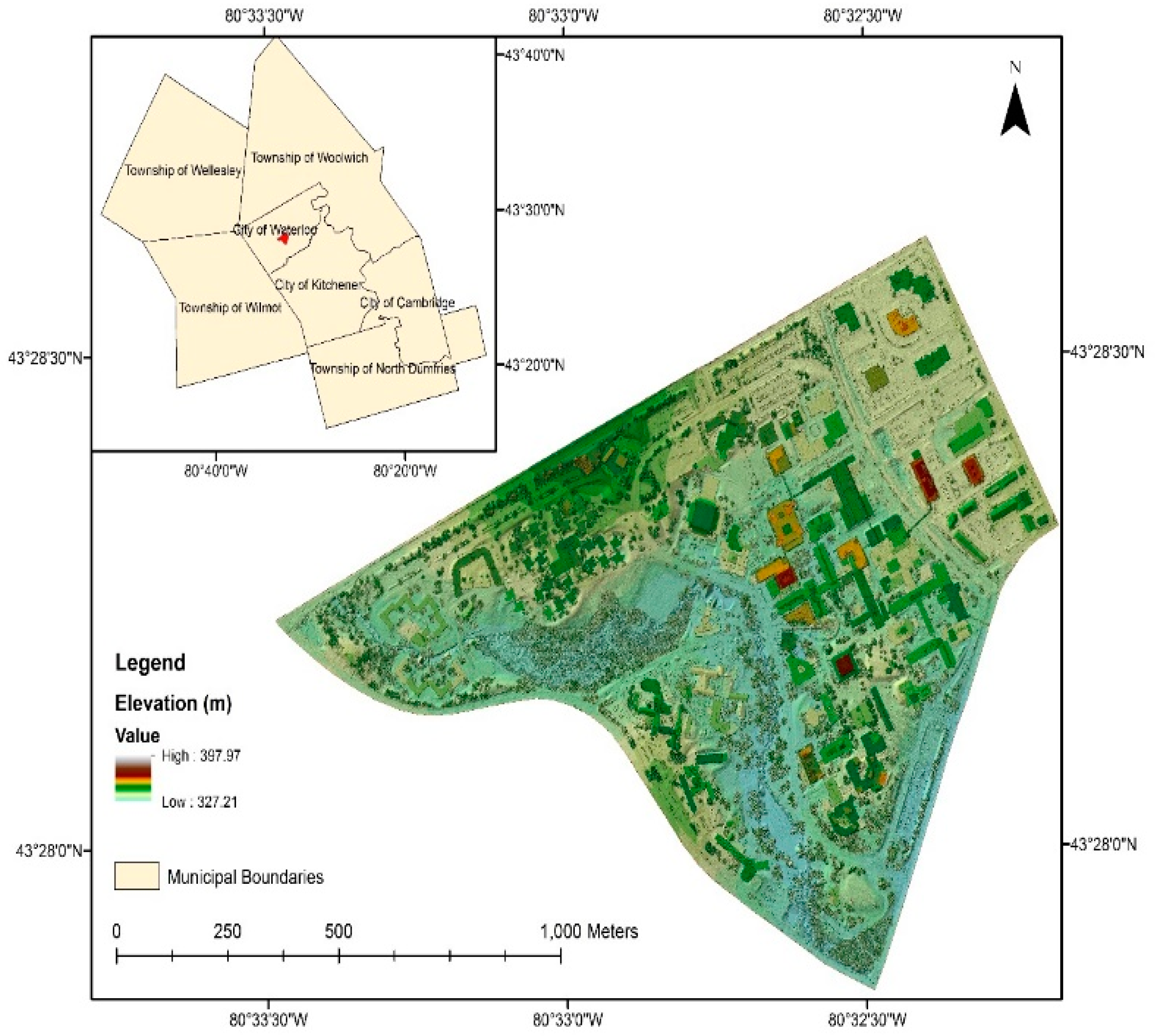
The study area is the main campus of the University of Waterloo, Ontario, Canada (Figure 1). The study area portrays a mixture of urban layout and forest environment, consisting of large buildings, roads, forests, lawns, parking lots, individual trees, bushes, a small lake, and a creek. The majority of the study area is flat, with some elevated regions in the northern part of the scene. The complexity of the ground objects and the mixture of low and high relief topography make this area suitable for DTM extraction analysis. The airborne LiDAR point clouds used in this study were a subset from the airborne LiDAR dataset acquired by the Leading Edge Geomatics team over the City of Waterloo using a RIEGL Q680i system during 2-3 November 2014. The system specifications are shown in Table 1. The average flying height was 1200 m above ground, producing LiDAR point clouds with a horizontal accuracy of approximately 31 cm (RMSE) and vertical accuracy of 6.1 cm (RMSE). The dataset contains a total of 3,082,000 points, which were inherently classified into five classes: ground, low vegetation, medium vegetation, high vegetation, and building. The classes were merged into two categories, ground and off-ground, to suit the purpose of this study.
3.2. DTM Extraction
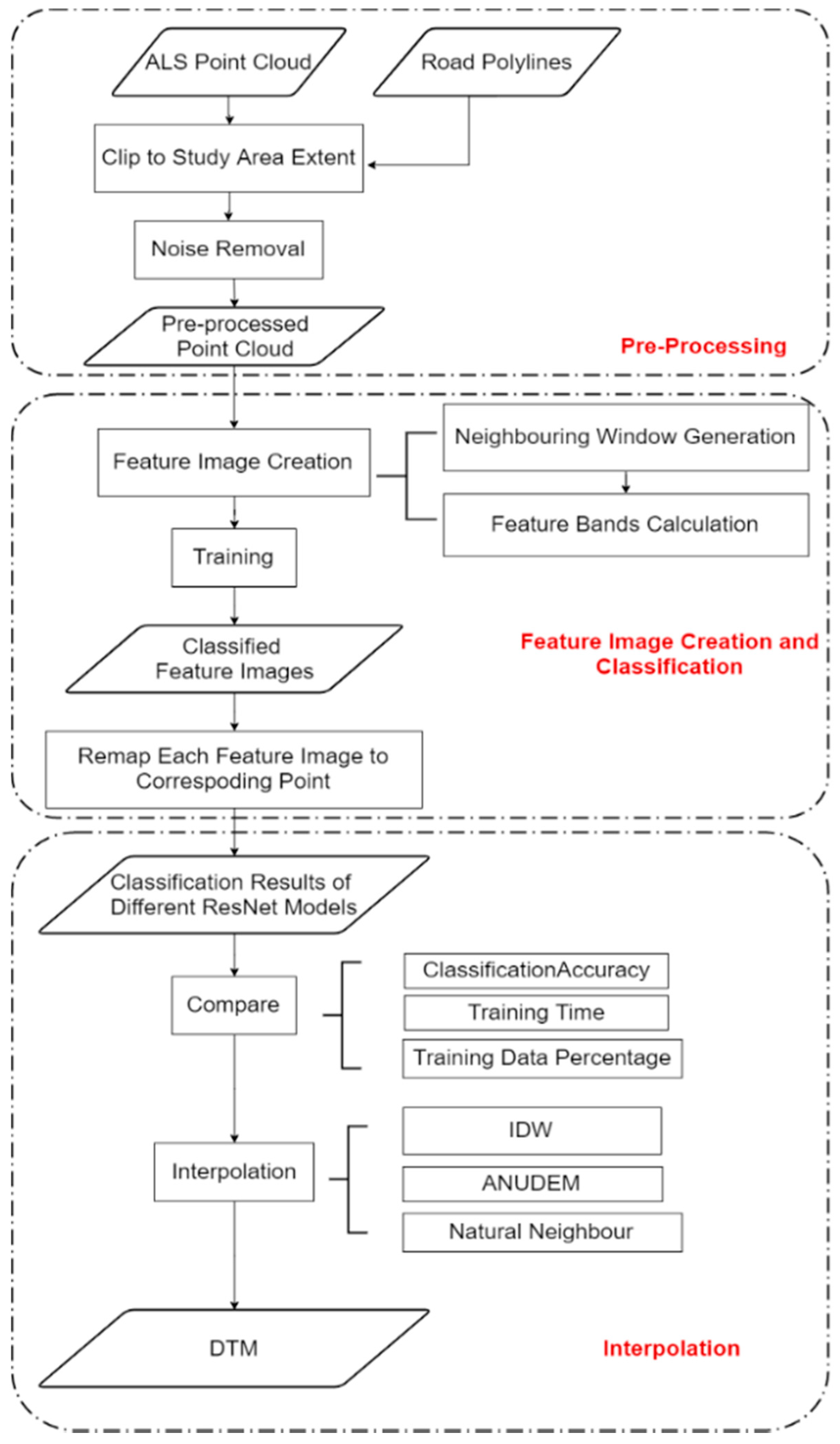
Figure 2 shows the general workflow of our method, which consists of three parts: data pre-processing, feature image creation and classification, and ground point interpolation. In pre-processing, the point cloud is clipped to the study area extent. Low outliers are removed at this stage using a statistical outlier removal (SOR) filter [39]. In the second part, each point is transformed into a featured image based on the height differences between neighboring points using the transformation proposed in Hu and Yuan (2016) [19]. Then, the feature images are classified using pretrained ResNet models. In the third step, the extracted ground points are interpolated to form a continuous elevation surface. The interpolated surfaces are assessed based on their RMSE from the ground truth.
3.3. Pre-Processing
During the pre-processing, the original airborne LiDAR point clouds were clipped to the extent of the defined study area. Then, before DTM extraction, the existing outliers in the raw point clouds need to be removed. Based on elevation, outliers can be categorized into low outliers and high outliers. Low outliers are the points that have extremely low elevation compared to their neighboring points. These points are typically caused by mechanical errors of the scanner or multiple reflections. Since the ground and non-ground points are mainly distinguishable by their elevation, low outliers are particularly destructive to the DTM extraction algorithm. Therefore, low outliers need to be removed during pre-processing. The SOR filter [39] was used for demonizing in CloudCompare. The filter computes the average distance between each point and its nearest neighbors (n = 6) in our study. Then, assuming the calculated distance distribution is normal, any point whose average distance with its 16 nearest neighbors is greater than the global average distance plus 3 standard deviations is rejected. The demonizing results in 1.88% of the original point clouds being removed.
3.4. Feature Image Generation
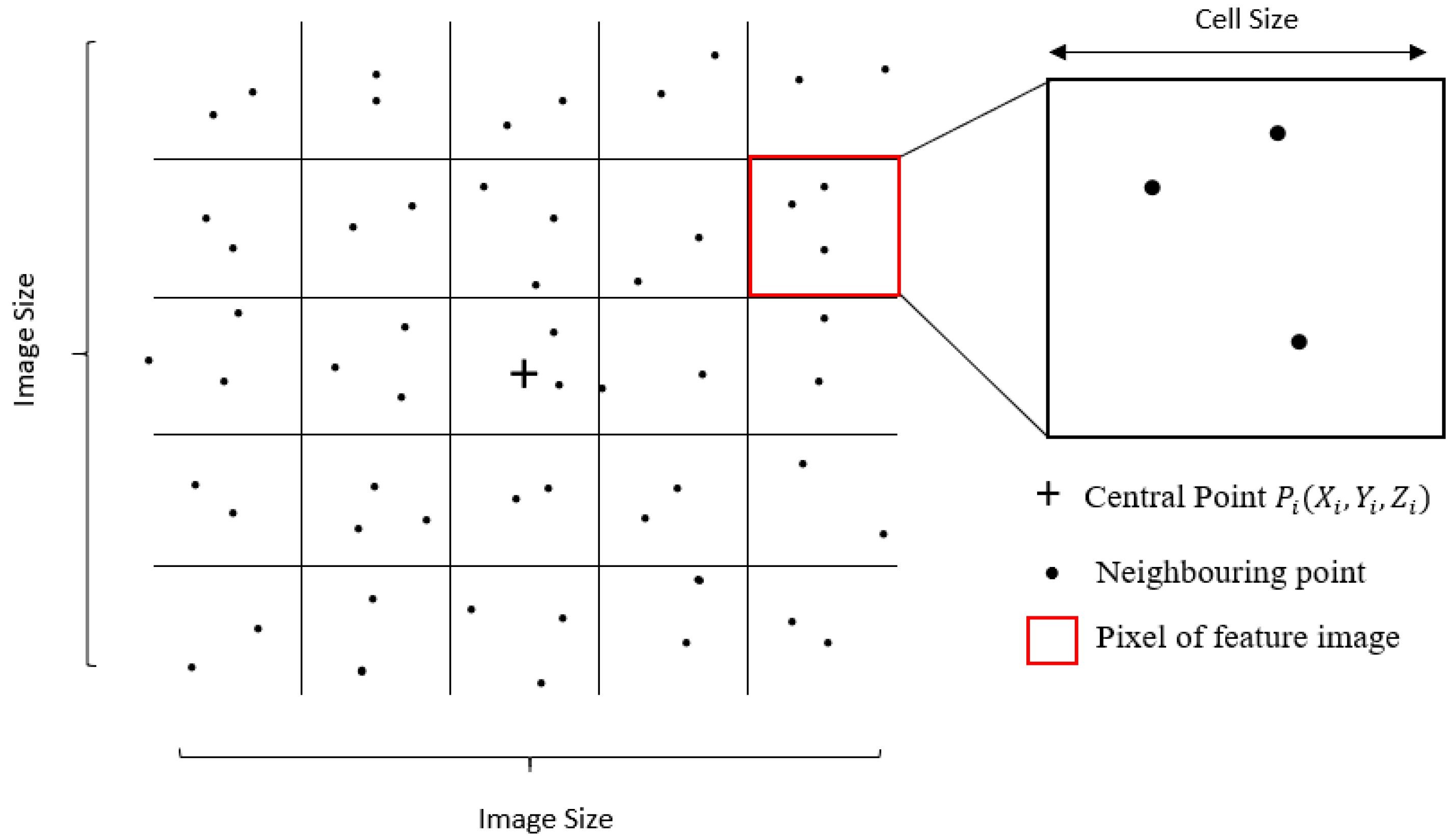
In order to determine whether a point is a ground or non-ground, not only the elevation of the point itself but also the spatial information of its neighboring points are needed. Most laser scanners also provide spectral information as auxiliary data, which were not accessible in our dataset. By turning the point cloud into a rasterized representation, each point classification will turn to label its corresponding feature image [40]. To this end, for each point , a corresponding image is generated based on the method proposed in Hu and Yuan, 2016 [19]. Figure 3 shows the workflow of point to image transformation, in which for each point in the point cloud, a corresponding feature image is generated based on its elevation difference with neighboring points.
The point is located at the center of this square window, and thus, it will be referred to as the central point. The square window is then partitioned into multiple cells based on two parameters: cell size and image size. Image size indicates the number of rows and columns of an image. Cell size indicates the resolution of feature image pixels, which should be set slightly larger than the average point spacing. Since the average point spacing of the point cloud is approximately 1 m, to avoid empty cells and make most of the abundant spatial information simultaneously, the cell size is chosen to be 1.5 m, which is slightly larger than the point spacing. The largest building in the dataset has a width of approximately 70 m. To identify such a building, a spatial context of approximately double the building size is needed. Thus, the image size is chosen to be 128 × 128 cells, which is equivalent to 192 × 192 m. Next, the maximum (), minimum (), and average () elevation within each cell is calculated. The last but critical step is to subtract from , , and to acquire pixel values for synthetic red, green, and blue bands; then, through sigmoid function, the elevation difference is mapped into three-pixel values between 0 and 255 using:
The following sigmoid function is used to take a number of as input and transforms it into a value between 0 and 1:
3.5. Feature Image Classification
The deep Residual Network (ResNet) [27] was chosen to perform the classification task due to its outstanding performance on the ImageNet dataset. Compared to plain networks, residual networks can perform well in much deeper architectures while maintaining lower computational complexity. With the increasing depth of the network, the training and testing accuracies first saturate and then decrease. Experimental results show that such a decrease in accuracy is not overfitting since both training and testing accuracy have simultaneously dropped. The residual networks are designed to ease the training of deep CNNs by adding residual learning blocks to the corresponding “plain” networks (networks that simply stack layers). Convolutional layers are the main calculating part of CNN, which uses kernels to transform input data into feature maps. They use kernels to connect to a local reception field in the previous layer (either an input image or an intermediate feature map). By sliding over the full extent of the input volume, the output feature map represents the filter response of the input image or feature maps.
A batch normalization (BN) is performed after each convolutional layer and before activation. BN is an effective way to accelerate learning and prevent overfitting. The input data in each mini-batch are normalized using:
where denotes the current batch, and are the mean and variance of the mini-batch, respectively, is a constant added to the mini-batch variance for numerical stability, and and are the parameters to be learned. A ReLU (Rectified Linear Unit) activation is used after BN to ensure nonlinearity. The ReLU activation function computes , which simply regards all values below zero as zero.
The pooling layers are also referred to as down-sampling layers. It usually follows one or several convolutional layers to reduce the dimension of the feature map. The pooling layer minimizes the dimension of feature maps by taking the average or maximum value within the kernel, thus reducing the network’s parameters, and has a certain effect in preventing overfitting. The neurons in fully connected layers are connected to every neuron in the previous layer. Fully connected layers are the last group of layers in ResNet, which outputs the probability of each input that belongs to a certain class by softmax activation function in its last layer. The dimension of the last fully connected layer depends on the number of classes to be predicted. In our case, the fully connected layer has two neurons, since the task is a binary classification problem.
3.6. Transfer Learning
The training was based on fine-tuning the ResNet models with pre-trained ImageNet weights on the feature images dataset. ResNet models with 18, 34, and 50 layers were adopted, referred to as ResNet18, ResNet34, and ResNet50, respectively. In order to overcome the size difference between feature images and ImageNet images, the top two layers of the network need to be modified, which are the average pooling layer and the fully connected layer. Since our problem is a binary classification problem, the fully connected layer was resized to (512, 2) for ResNet18 and -34 and (2048, 2) for ResNet50. The second last layer, which is the average pooling layer, has a kernel size of 4 and stride 1. Cross-Entropy Loss is used to measuring the loss of the neural network. Our aim was to minimize the loss, i.e., the smaller the loss is, the better the model will be. The loss is calculated by:
where is the predicted probability of an input belong to its true class, is the label of current input, and is the batch size. The training was performed on a computer with an NVIDIA GeForce GTX 1080 GPU, an Intel CPUi7-9700k 3.6 GHz with 8 cores, and 32 GB of RAM.
3.7. Interpolation
Interpolation is the process of transforming the extracted ground points into a continuous surface representing terrain elevation. The three following interpolation methods are employed and compared to minimize the RMSE: Inverse Distance Weighting (IDW), ANUDEM (Australian National University DEM), and Natural Neighbor.
IDW is a deterministic interpolation method that predicts the value at location using:
where is the number of neighboring points, is the elevation of ith neighboring point, is the distance between the ith neighboring point and location , and is the power of distance. The value of is essentially a distance-weighted average of .
IDW explicitly makes the assumption that things nearer are more similar than things apart; thus, measured points that are spatially closer to the interpolated location will be assigned higher weights. The method is essentially a distance-weighted average approach: as the distance between the measured point and the interpolating location increases, the inverse of the distance decreases and, therefore, the weight. The power adjusts the speed of the weights, which diminishes with distance. If , Equation (7) will calculate a simple average of the neighboring points’ Z values. As increases, the weights of distant points will decrease rapidly. IDW is an exact interpolator, which means that the interpolated value will not exceed the minimum or maximum of the elevations used to predict the interpolated value.
ANUDEM is an interpolation method that creates grid DEM using locally adaptive elevation gridding [41]. Although this method is designed to work with drainage structure and hydrologically relevant topographic data [42], it can also produce outstanding quality DEMs with regular elevation point data. ANUDEM uses a spline fitting method that is computationally efficient and can work with an arbitrarily large dataset. A multi-grid method is proposed to generate the DEM starting from the coarse grid, then refined the resolution on a successive finer grid.
Natural neighbor, also known as “area-stealing” interpolation, is an exact interpolator. The predicted values do not exceed the minimum and maximum values of input elevations. Similar to IDW, the natural neighbor method does not infer any trend from the input data. Instead, it only considers the elevation value of the interpolating location’s direct neighbors and derives predicted values using the weighted average. The key component in natural neighbor interpolation is the Voronoi diagram, which corresponds to the Delaunay triangulation in terms that the Voronoi diagram can be produced by connecting all the circumcircles centers of the Delaunay triangulations. First, a Voronoi diagram is created for each of the elevation points. Then, for every location that needs to be interpolated, a Voronoi polygon is created. Next, points , whose Voronoi polygon overlaps with the polygon of location , are defined as ’s natural neighbors. Weights are assigned to the natural neighbors based on the overlapping area between the Voronoi polygon of and the polygons of . The predicted value at will be the weighted average of its natural neighbors’ Z-values.
4. Results
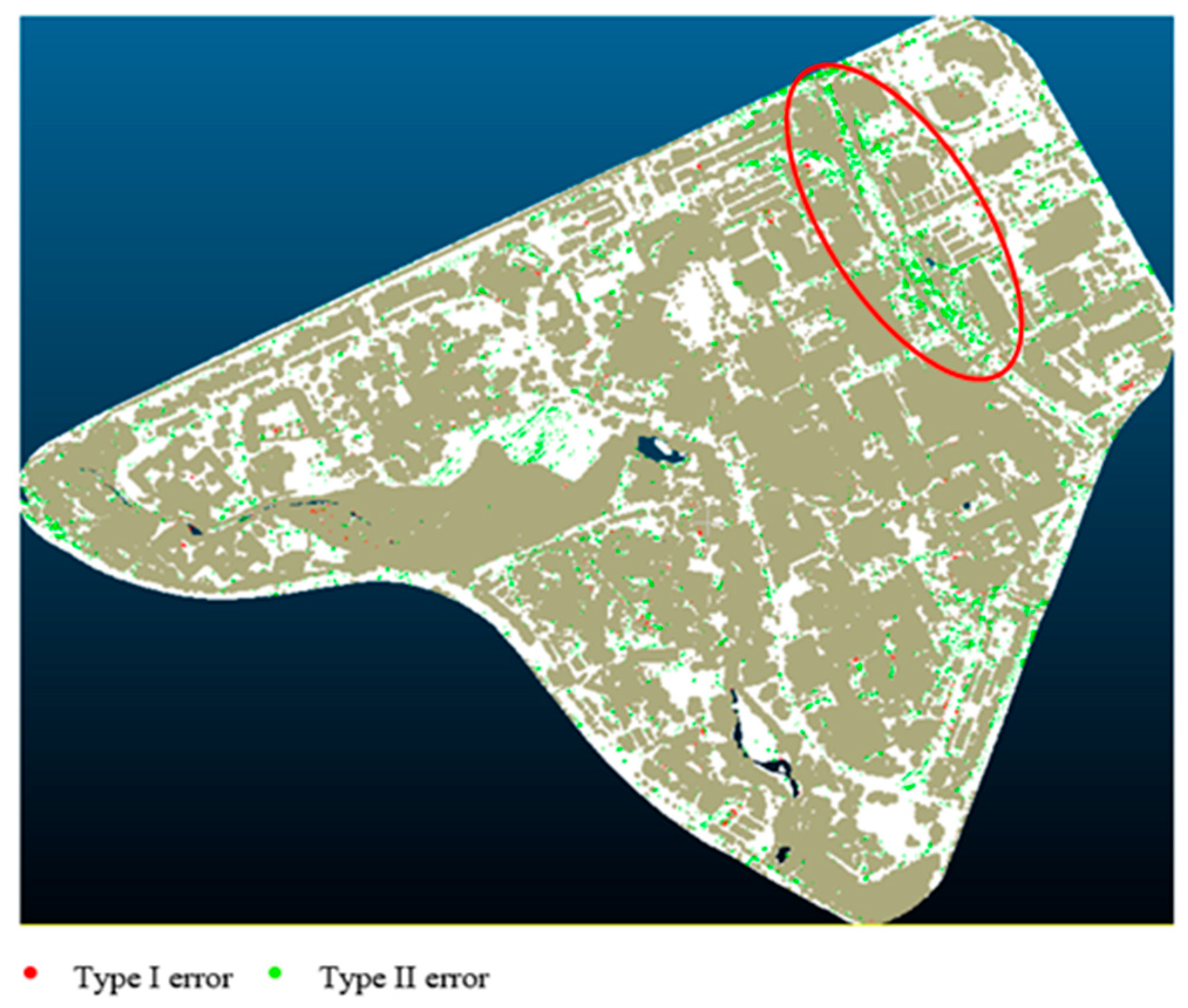
Through extensive experiments, increasing the complexity of the model and increasing the amount of training data does not significantly improve the classification result, so the simplest model with the least training data is chosen due to the efficiency in training time and low labeling requirement. Thus, the combination of ResNet 18 and 10% of training data is considered optimal. The classification result is presented in Figure 4.
Type I and Type II errors are common measurements for DTM classification accuracy. Type I error indicates the misclassification of the ground as non-ground, and Type II error is the misidentification of off-ground objects as ground. In Figure 4, the red pixels indicate the occurrence of Type I errors, while the green pixels indicate the occurrence of Type II errors. Very little Type I error is presented in the scene. That means the terrain points are largely preserved. On the other hand, a few Type II errors can be observed, especially along the railway (highlighted by eclipse), where the occurrence of shrubs tends to be misclassified as ground.
Two zoomed-in scenes are selected to visually present the filtering details. Shaded images of DSM and DTM are created for better visualization. Figure 5 illustrates the filtering results of buildings, roadside trees, and cars in parking lots. Figure 6 shows the filtering results of dense vegetation. It can be seen that most of the off-ground objects are correctly removed, while the terrain characteristics are preserved.
The confusion matrix is shown in Table 2. The proposed method can achieve high classification accuracy. The percentages of Type I, Type II, and the total error are 0.52%, 4.84%, and 2.43%, respectively. Additionally, the system is biased towards making Type II errors, which is favorable. According to Sithole et al. (2004) [38], filters should strive to minimize Type I errors, since Type II errors are caused by misidentifying off-ground objects as ground. Such errors are typically conspicuous and are relatively easier to remove. On the other hand, Type I errors are the misclassification of the ground as non-ground, which results in terrain reconstruction gaps and is, thus, difficult to correct.
5. Discussions
5.1. Impact of Pre-Trained Weights
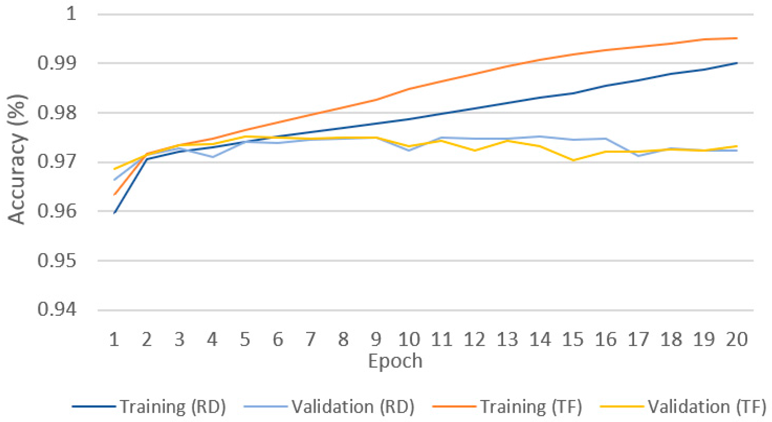
In order to investigate whether using pretrained model accelerates the training process, we trained and compared the models from both random initialized (RD) and transferred (TF) weights. The evaluation was conducted by comparing the true labels done manually and the results achieved by each implemented method. Figure 7 shows the training and validation accuracy achieved using 10% of the training data on ResNet18. Although the pretrained model achieved higher training accuracy throughout the training process, we can observe a little difference in validation accuracy. The model using transferred weights achieved higher validation accuracy than the random initialized model in the first five epochs, which was consistent for all subsequent epochs. This indicates a stronger generalization ability of our proposed ResNet. However, their difference has a negligible amount of 0.003.
5.2. Comparison of Different ResNet Models
Three ResNet models are used in this study: ResNet18, ResNet34 and ResNet50. As the depth of the network increases, it is capable of representing more complex features. However, the computational time as well as required memory and storage space are also increasing. Moreover, complex networks may overfit the training dataset and fail to generalize well to other datasets. Thus, to select the optimal network, three ResNet models are compared with four different training data rates (10%, 20%, 30%, and 40%), while the validation percentage is held constant at 10%.
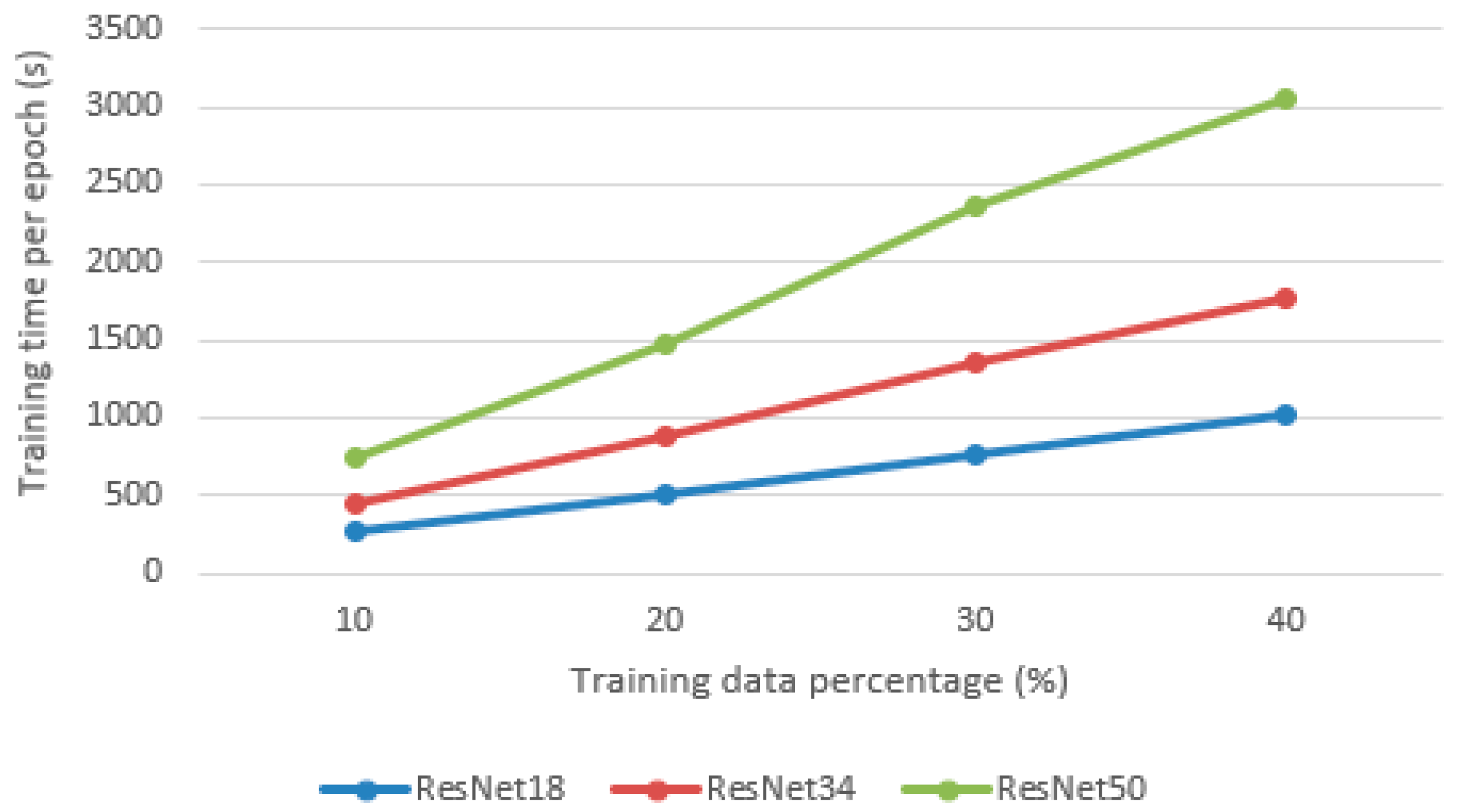
After experimenting on the validation dataset, a learning rate of 0.001 and drop out of 0.2 are chosen to train the models. As shown in Figure 8, the validation accuracy of the three models does not differ significantly, which means ResNet18 is sufficient for the classification task. On the other hand, adding more training data can effectively improve the validation accuracy. With 10% of the training data, the average accuracy achieved by three models is 97.49%, while with 40% of the training data, the average accuracy achieved is 97.89%. However, this improvement is relatively trivial, since the validation accuracy only improves 0.04%, which indicates a slight improvement in reducing the number of misclassified points. The computational cost (time) for training each model is shown in Figure 9. It can be seen that as the number of layers increases, the training times also increase. While ResNet18 and ResNet50 yield similar results, the amount of time used to train ResNet50 is almost tripled. Thus, ResNet18 is the best model, since it provides similar results to ResNet50 in a shorter time. Training time increases linearly with the amount of input data. For ResNet18, 34, and 50, the time used to train one epoch on 10% of the data is 4 m 25 s, 7 m 33 s, and 12 m 27 s, respectively.
5.3. Comparative Studies
We compared the proposed method with two traditional filters, namely the Progressive Morphological Filter (PMF) [29] and Progressive TIN Densification filter (PTD) [22]. The comparison was conducted based on three criteria: classification accuracy, RMSE of interpolated DTM, and qualitative results.
Table 3 illustrates the point-wise classification accuracy of each model. The Type I, Type II, and the total error of ResNet are 0.52%, 4.84% and 2.43%, while the errors for PTD are 1.55%, 5.37%, and 3.22% and for PMF 7.82%, 11.62%, and 9.48%, respectively. It can be seen that the ResNet model produces the lowest error rates.
RMSE is another index that reflects the quality of the DTM. After ground points are extracted, raster DTMs are generated using interpolation. Three interpolation techniques are compared: IDW, ANUDEM, and natural neighbor. The RMSEs of interpolated DTMs are shown in Table 4.
It is not surprising to see that the RMSE results are consistent with point classification accuracy. DTMs generated by ResNet extracted points also have the lowest RMSE, which is less than 10 cm. DTMs generated by PTD extracted points have slightly higher RMSE, while DTMs generated by PMF extracted points have RMSEs almost three times higher. Among the three interpolation methods, natural neighbor yields the best result for ResNet- and PTD-extracted points, while ANUDEM yields the best result for PMF extracted points. Qualitative assessment is made to examine the filter performances for different non-ground objects. Certain terrain characteristics are identified as difficult to filter for all DTM filtering techniques based on visual inspection, such as complex building structure, low vegetation, and attached objects (buildings connected with or built into the ground). Based on the RMSE analysis, each filter extracted points are interpolated using the most suitable interpolation technique.
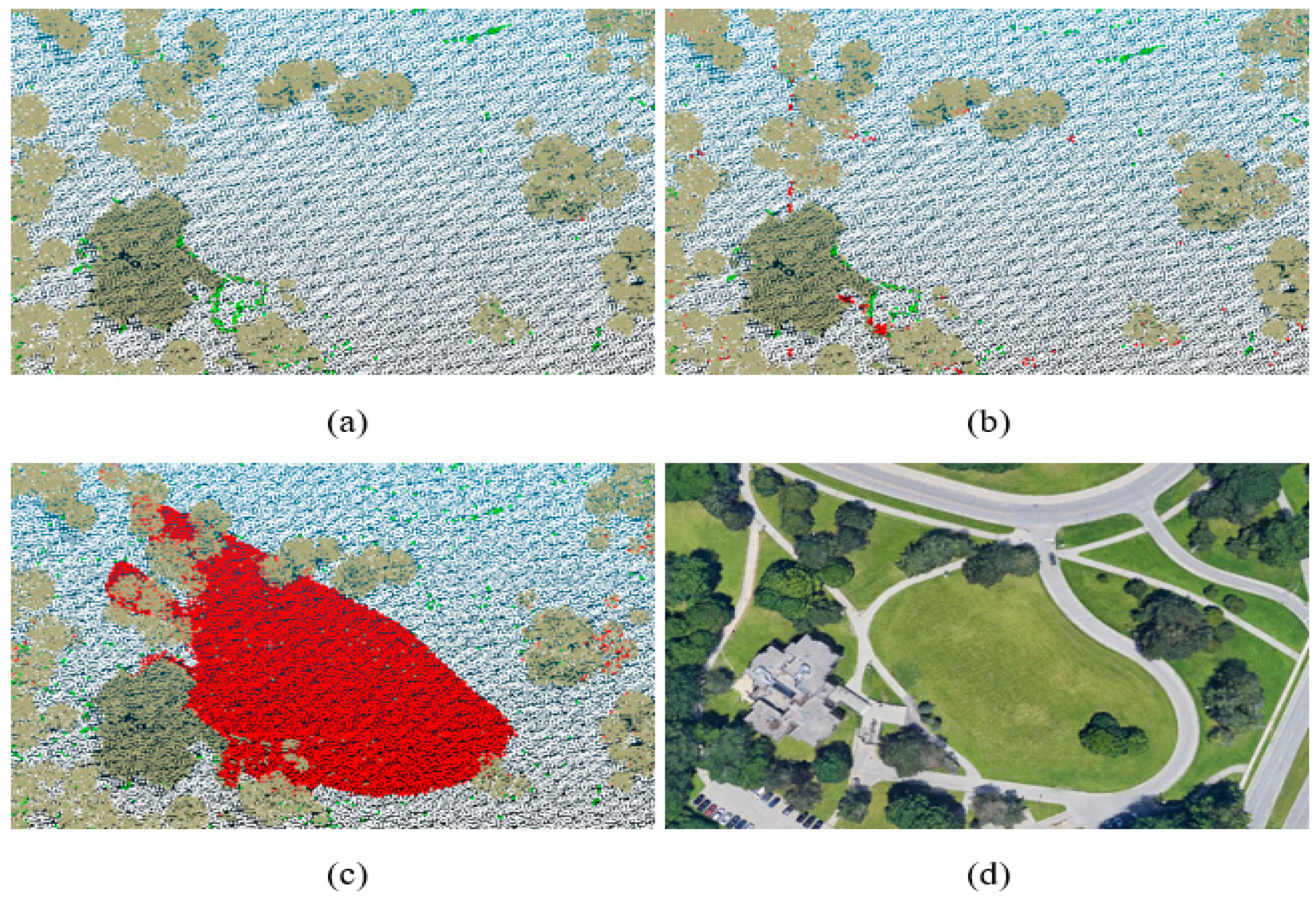
5.4. Vegetation and Buildings in Sloped Areas
Sloped areas with vegetation or building on top are difficult to filter due to the large variability in slope and terrain discontinuity caused by vegetation or building blockage. This type of terrain is challenging for the PMF filter in terms of classification, which assumes a constant slope for the entire study area. Figure 10 shows the filters’ performances in a sloped area with trees near a building. It can be seen that both ResNet and PTD yield only a few errors by misclassified curbs and grass (shows in green color), while PMF misidentified a large part of the terrain as non-ground (shows in red color).
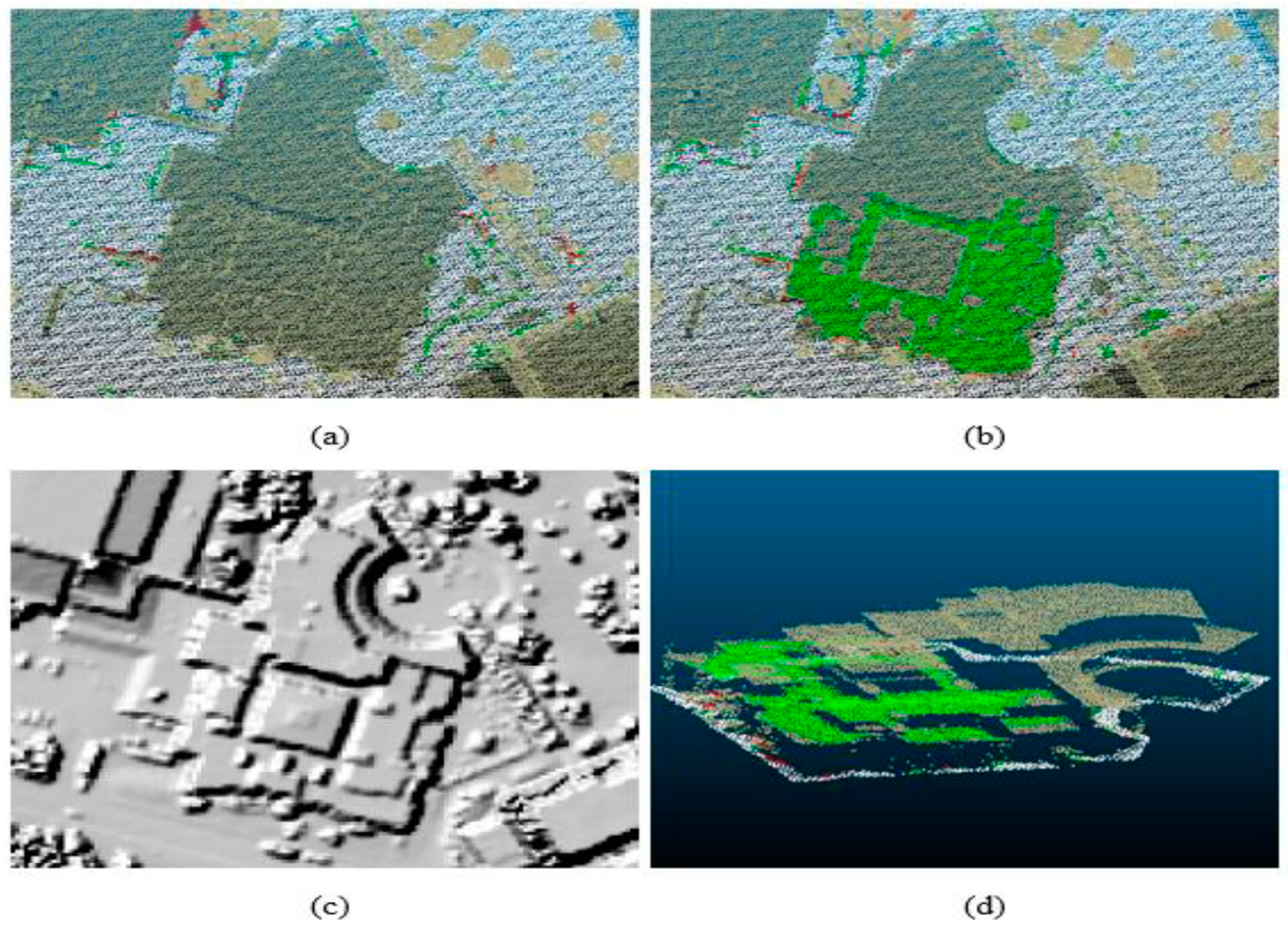
5.5. Complex Structures
PTD filter encounters difficulties with complex buildings with rooftops at different heights. An example of such a building structure is shown in Figure 11. The building rooftops are at three different elevations, while the two lower parts of the rooftop are misidentified as ground by the PTD filter. The ResNet filter performs well in this situation since it considers a point’s direct neighbors and the elevation difference to all points within 196 m distance. The sufficient spatial information passed through point to image transformation enables the filter to detect building rooftops even when higher objects are presented in the scene.
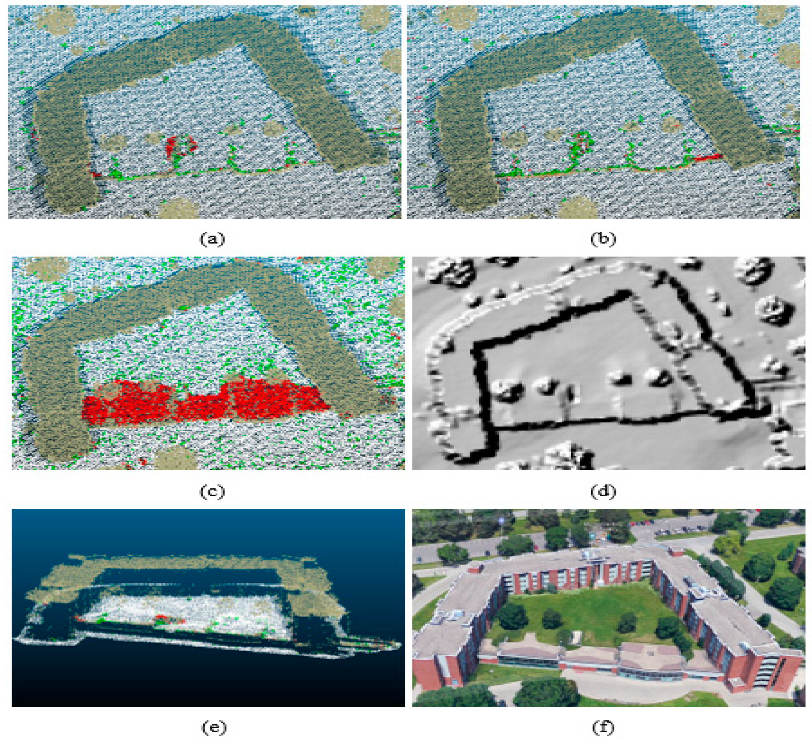
5.6. Mixed Buildings and Terrain
Special cases of buildings connected with or built into terrain make it difficult to define the boundary of ground and non-ground (see Figure 12). A part of the building is built into the terrain, making the building rooftop level with the inner ground. There are three options for classifying this type of structure. Option 1 is to keep the inner ground and remove all the buildings. Option 2 is to keep the rooftop and the inner ground while removing only the front building façade. Option 3 is to remove the entire building as well as the inner ground. The ground truth label adopts the second option, since it preserves most of the spatial information while introducing little error.
Both ResNet and PTD filters abide by the second option: to classify the rooftop and the inner ground as bare earth. However, even though the trees on the ground are removed, the rooftop handrail was misclassified as ground. The PMF complies with the second option; as shown in Figure 12c, the front building rooftop is all classified as non-ground.
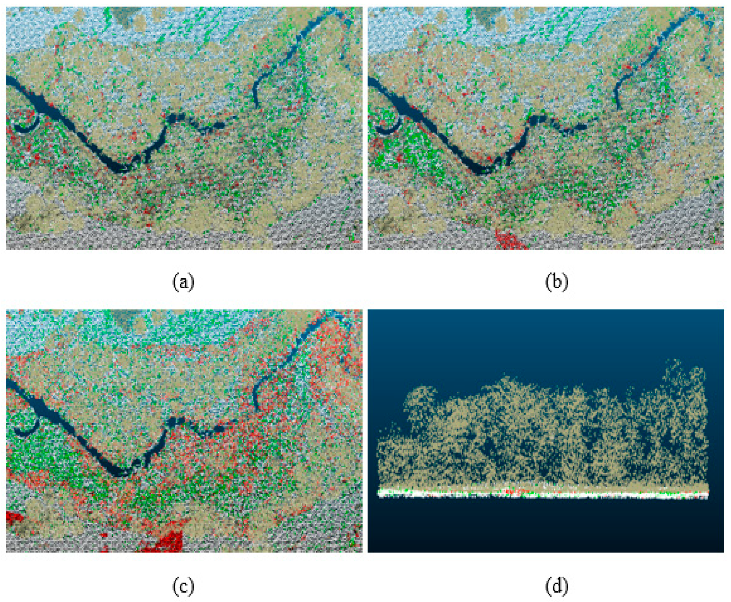
5.7. Dense Vegetation
All three filters perform worse when identifying terrain in the densely vegetated area. As shown in Figure 13, large quantities of Type I and Type II errors can be observed in all three cases. However, based on the front view image, high vegetation is correctly classified. The source of the errors comes from failing to differentiate between low vegetation and bare ground. It is challenging to differentiate these two classes based only on the height attribute, especially in densely vegetated areas where there is the vegetation of various heights. A possible solution for this case is to use multispectral LiDAR. With the aid of spectral information, vegetation and ground can be easily distinguished with high accuracy estimates [4].
6. Conclusions
This study presented a workflow for DTM generation using airborne LiDAR data based on CNN and transfer learning for a small area covering the main campus of the University of Waterloo region. The proposed workflow was tested using the real airborne LiDAR point clouds. To cope with the unstructured point clouds and CNN’s requirement of organized input data, we conducted a point-to-image transformation. Each LiDAR point of interest with its neighboring points was transformed into a featured image based on the elevation differences. The feature images were used as input for the ResNet models. The ground points can be extracted by remapping the classified feature images to their corresponding points in the airborne LiDAR point clouds. The proposed workflow was then compared with two traditional filers (PTD and PMF) in terms of point-wise classification accuracy, RMSE of interpolated DTM, and quantitative performance in several special cases. Results concluded that the proposed workflow could produce high-quality DTMs with Type I error, Type II error, and a total error of 0.89%, 3.62%, and 2.10%, respectively. Moreover, by using pretrained weights on ImageNet, the model can achieve high accuracy using only a small percentage of training data. Further analysis of interpolated DTMs revealed that the RMSE of the proposed workflow is 7.3 cm, compared with 9.4 cm produced by PTD and 26 cm produced by PMF. Several special cases that are particularly difficult to filter are presented and discussed. The proposed workflow performed well in most of these cases, except for densely vegetated regions, where the distribution of Type I and Type II errors can be observed. Finally, the proposed model can be used in various disciplines such as transportation, urban planning, and geology in low- to medium-density urban regions covered by less canopy. The authors will work on more data and a larger area in the future study to see the accountability and applicability of the developed algorithm.
Author Contributions
Conceptualization, H.L. and J.L. (Jonathan Li); methodology, H.L., W.Y., J.L. (Jun Liu), S.P., W.T., S.N.F., and J.L. (Jonathan Li); software, H.L., W.Y., J.L. (Jun Liu), and J.L. (Jonathan Li); validation, H.L., W.Y., J.L. (Jun Liu), S.P., and J.L. (Jonathan Li); formal analysis, H.L. and W.Y.; investigation, H.L., W.Y., J.L. (Jun Liu), J.L. (Jonathan Li), and S.P.; resources, H.L., W.Y., J.L. (Jun Liu), S.P., S.N.F., and J.L. (Jonathan Li); data curation, H.L., W.Y., and J.L. (Jonathan Li); writing—original draft preparation, H.L. and J.L. (Jonathan Li); writing—review and editing, H.L., S.P., J.L. (Jonathan Li), W.Y., W.T., and S.N.F., visualization, H.L., J.L. (Jun Liu), S.P., and J.L. (Jonathan Li); supervision, J.L. (Jonathan Li); project administration, H.L., W.Y., J.L. (Jun Liu), S.P., and J.L. (Jonathan Li); funding acquisition, H.L. and J.L. (Jun Liu). All authors have read and agreed to the published version of the manuscript.
Funding
This work was supported in part by the National Natural Science Foundation of China under Grant No. 6194100039, the Natural Science Foundation of Zhejiang Province under Grant No. LHQ20F020001, and the Basic Public Welfare Research Project of Zhejiang Province under Grant No. LGG18F030003.
Data Availability Statement
Data is available upon request.
Acknowledgments
This study was carried out as part of the proposed joint research to build a foundation for working together to support Sustainable Development Goal (SDG)-17 and develop possibilities for the authors with international University collaborators.
Conflicts of Interest
The authors declare no conflict of interest.
References
- Dorninger, P.; Pfeifer, N. A comprehensive automated 3D approach for building extraction, reconstruction, and regularization from airborne laser scanning point clouds. Sensors 2008, 8, 7323–7343. [Google Scholar] [CrossRef] [Green Version]
- Chen, X.; Chengming, Y.; Li, J.; Chapman, M.A. Quantifying the carbon storage in urban trees using multispectral ALS data. IEEE J. Sel. Top. Appl. Earth Obs. Remote Sens. 2018, 11, 3358–3365. [Google Scholar] [CrossRef]
- Jochem, A.; Höfle, B.; Rutzinger, M.; Pfeifer, N. Automatic roof plane detection and analysis in airborne lidar point clouds for solar potential assessment. Sensors 2009, 9, 5241–5262. [Google Scholar] [CrossRef]
- Matikainen, L.; Karila, K.; Hyyppä, J.; Puttonen, E.; Litkey, P.; Ahokas, E. Feasibility of multispectral airborne laser scanning for land cover classification, road mapping and map updating. Int. Arch. Photogramm. Remote Sens. Spat. Inf. Sci. 2017, 42, 119–122. [Google Scholar] [CrossRef] [Green Version]
- Ministry of Natural Resources and Forestry. Southwestern Ontario Orthophotography Project (SWOOP). Digital Elevation Model User Guide. 2015. Available online: https://uwaterloo.ca/library/geospatial/sites/ca.library.geospatial/files/uploads/files/swoop_2015_dem_-_user_guide.pdf (accessed on 30 January 2021).
- Natural Resources Canada. High Resolution Digital Elevation Model (HRDEM)-CanElevation-Series Product Specifications. 2019. Edition 1.3. Available online: https://ftp.maps.canada.ca/pub/elevation/dem_mne/highresolution_hauteresolution/HRDEM_Product_Specification.pdf (accessed on 30 January 2021).
- Liu, X. Airborne LiDAR for DEM generation: Some critical issues. Progr. Phy. Geog. 2008, 32, 31–49. [Google Scholar]
- Hui, Z.; Li, D.; Jin, S.; Ziggah, Y.Y.; Wang, L.; Hu, Y. Automatic DTM extraction from airborne LiDAR based on expectation-maximization. Opt. Laser Technol. 2019, 112, 43–55. [Google Scholar] [CrossRef]
- Guan, H.; Li, J.; Yu, Y.; Zhong, L.; Ji, Z. DEM generation from lidar data in wooded mountain areas by cross-section-plane analysis. Int. J. Remote Sens. 2014, 35, 927–948. [Google Scholar] [CrossRef]
- Li, Y.; Wu, H.; Xu, H.; An, R.; Xu, J.; He, Q. A gradient-constrained morphological filtering algorithm for airborne LiDAR. Opt. Laser Technol. 2013, 54, 288–296. [Google Scholar] [CrossRef]
- Li, Y.; Yong, B.; Wu, H.; An, R.; Xu, H. An improved top-hat filter with sloped brim for extracting ground points from airborne lidar point clouds. Remote Sens. 2014, 6, 12885–12908. [Google Scholar] [CrossRef] [Green Version]
- Hui, Z.; Hu, Y.; Yevenyo, Y.Z.; Yu, X. An improved morphological algorithm for filtering airborne LiDAR point cloud based on multi-level kriging interpolation. Remote Sens. 2016, 8, 35. [Google Scholar] [CrossRef] [Green Version]
- Chen, Z.; Gao, B.; Devereux, B. State-of-the-art: DTM generation using airborne LiDAR data. Sensors 2017, 17, 150. [Google Scholar] [CrossRef] [Green Version]
- Wang, X.; Ma, X.; Yang, F.; Su, D.; Qi, C.; Xia, S. Improved progressive triangular irregular network densification filtering algorithm for airborne LiDAR data based on a multiscale cylindrical neighborhood. Appl. Opt. 2020, 59, 6540–6550. [Google Scholar] [CrossRef] [PubMed]
- Ni, H.; Lin, X.; Zhang, J.; Chen, D.; Peethambaran, J. Joint clusters and iterative graph cuts for ALS point cloud filtering. IEEE J. Sel. Top. Appl. Earth Obs. Remote Sens. 2018, 11, 990–1004. [Google Scholar] [CrossRef]
- Sánchez, M.; Váquez Álvarez, A.; López Vilariño, D.; Fernández Rivera, F.; Cabaleiro Domínguez, J.C.; Fernández Pena, T. Fast ground filtering of airborne LiDAR data based on iterative scan-line spline interpolation. Remote Sens. 2019, 11, 2256. [Google Scholar] [CrossRef] [Green Version]
- Shi, W.; Ahmed, W.; Wu, K. Morphologically iterative triangular irregular network for airborne LiDAR filtering. J. Appl. Remote Sens. 2020, 14, 034525. [Google Scholar]
- Meng, X.; Currit, N.; Zhao, K. Ground filtering algorithms for airborne LiDAR data: A review of critical issues. Remote Sens. 2010, 2, 833–860. [Google Scholar] [CrossRef] [Green Version]
- Hu, X.; Yuan, Y. Deep-learning-based classification for DTM extraction from ALS point cloud. Remote Sens. 2016, 8, 730. [Google Scholar] [CrossRef] [Green Version]
- Qi, C.R.; Yi, L.; Su, H.; Guibas, L.J. Pointnet++: Deep hierarchical feature learning on point sets in a metric space. In Proceedings of the Advances in Neural Information Processing Systems 30: Annual Conference on Neural Information Processing Systems 2017, Long Beach, CA, USA, 4–9 December 2017. [Google Scholar]
- Zhang, W.; Qi, J.; Wan, P.; Wang, H.; Xie, D.; Wang, X.; Yan, G. An easy-to-use airborne LiDAR data filtering method based on cloth simulation. Remote Sens. 2016, 8, 501. [Google Scholar] [CrossRef]
- Axelsson, P. DEM generation from laser scanner data using adaptive TIN models. Int. Arch. Photogramm. Remote Sens. 2000, 33, 110–117. [Google Scholar]
- Kraus, K.; Pfeifer, N. Determination of terrain models in wooded areas with airborne laser scanner data. ISPRS J. Photogramm. Remote Sens. 1998, 53, 193–203. [Google Scholar] [CrossRef]
- Zhang, J.; Lin, X. Filtering airborne LiDAR data by embedding smoothness-constrained segmentation in progressive TIN densification. ISPRS J. Photogramm. Remote Sens. 2013, 81, 44–59. [Google Scholar] [CrossRef]
- Chen, Q.; Wang, H.; Zhang, H.; Sun, M.; Liu, X. A point cloud filtering approach to generating DTMs for steep mountainous areas and adjacent residential areas. Remote Sens. 2016, 8, 71. [Google Scholar] [CrossRef] [Green Version]
- He, Y.; Zhang, C.; Fraser, C.S. Progressive filtering of airborne LiDAR point clouds using graph cuts. IEEE J. Sel. Top. Appl. Earth Obs. Remote Sens. 2018, 11, 2933–2944. [Google Scholar] [CrossRef]
- He, K.; Zhang, X.; Ren, S.; Sun, J. Deep residual learning for image recognition. In Proceedings of the 2016 IEEE Conference on Computer Vision and Pattern Recognition, Las Vegas, NV, USA, 26 June–1 July 2016. [Google Scholar] [CrossRef] [Green Version]
- Shao, Y.-C.; Chen, L.-C. Automated searching of ground points from airborne lidar data using a climbing and sliding method. Photogramm. Eng. Remote Sens. 2008, 74, 625–635. [Google Scholar] [CrossRef] [Green Version]
- Zhang, K.; Chen, S.-C.; Whitman, D.; Shyu, M.-L.; Yan, J.; Zhang, C. A progressive morphological filter for removing nonground measurements from airborne LiDAR data. IEEE Trans. Geosci. Remote Sens. 2003, 41, 872–882. [Google Scholar] [CrossRef] [Green Version]
- Yang, Z.; Tan, B.; Pei, H.; Jiang, W. Segmentation and multi-scale convolutional neural network-based classification of airborne laser scanner data. Sensors 2018, 18, 3347. [Google Scholar] [CrossRef] [PubMed] [Green Version]
- Gevaert, C.; Persello, C.; Nex, F.; Vosselman, G. A deep learning approach to DTM extraction from imagery using rule-based training labels. ISPRS J. Photogramm. Remote Sens. 2018, 142, 106–123. [Google Scholar] [CrossRef]
- Luo, Y.; Ma, H.; Zhou, L. DEM retrieval from airborne LiDAR point clouds in mountain areas via deep neural networks. IEEE Geosci. Remote Sens. Lett. 2017, 14, 1770–1774. [Google Scholar] [CrossRef]
- Wen, C.; Yang, L.; Li, X.; Peng, L.; Chi, T. Directionally constrained fully convolutional neural network for airborne LiDAR point cloud classification. ISPRS J. Photogramm. Remote Sens. 2020, 162, 50–62. [Google Scholar] [CrossRef] [Green Version]
- Li, W.; Wang, F.-D.; Xia, G.-S. A geometry-attentional network for ALS point cloud classification. ISPRS J. Photogramm. Remote Sens. 2020, 164, 26–40. [Google Scholar] [CrossRef]
- Li, X.; Wang, L.; Wang, M.; Wen, C.; Fang, Y. DANCE-NET: Density-aware convolution networks with context encoding for airborne LiDAR point cloud classification. ISPRS J. Photogramm. Remote Sens. 2020, 166, 128–139. [Google Scholar] [CrossRef]
- Zhao, C.; Guo, H.; Lu, J.; Yu, D.; Li, D.; Chen, X. ALS point cloud classification with small training data set based on transfer learning. IEEE Geosci. Remote Sens. Lett. 2019, 17, 1406–1410. [Google Scholar] [CrossRef]
- Zhao, R.; Pang, M.; Wang, J. Classifying airborne LiDAR point clouds via deep features learned by a multi-scale convolutional neural network. Int. J. Geog. Inf. Sci. 2018, 32, 960–979. [Google Scholar] [CrossRef]
- Sithole, G.; Vosselman, G. Experimental comparison of filter algorithms for bare-Earth extraction from airborne laser scanning point clouds. ISPRS J. Photogramm. Remote Sens. 2004, 59, 85–101. [Google Scholar] [CrossRef]
- Rusu, R.B.; Marton, Z.C.; Blodow, N.; Dolha, M.; Beetz, M. Towards 3D point cloud based object maps for household environments. Robot. Auton. Syst. 2008, 56, 927–941. [Google Scholar] [CrossRef]
- Winiwarter, L.; Mandlburger, G.; Schmohl, S.; Pfeifer, N. Classification of ALS point clouds using end-to-end deep learning. PFG J. Photogramm. Remote Sens. Geoinf. Sci. 2019, 87, 75–90. [Google Scholar] [CrossRef]
- Hutchinson, M.F.; Xu, T.; Stein, J.A. Recent progress in the ANUDEM elevation gridding procedure. Geomorphometry 2011, 2011, 19–22. [Google Scholar]
- Pirasteh, S.; Li, J. Developing an algorithm for automated geometric analysis and classification of landslides incorporating LiDAR-derived DEM. Environ. Earth Sci. 2018, 77, 414. [Google Scholar] [CrossRef]
Figure 1.
The study area covering the main campus of the University of Waterloo.

Figure 2.
General workflow of our method.

Figure 3.
Point-to-feature image transformation.

Figure 4.
Classification results. Red color shows Type I errors and green color shows Type II errors.
Figure 4.
Classification results. Red color shows Type I errors and green color shows Type II errors.

Figure 5.
Buildings before (left) and after (right) filtering for roadside trees and cars in parking lots.
Figure 5.
Buildings before (left) and after (right) filtering for roadside trees and cars in parking lots.

Figure 6.
Vegetation before (left) and after (right) filtering.

Figure 7.
Impact of pretrained weights.

Figure 8.
Comparison of validation accuracies.

Figure 9.
Training times of different models.

Figure 10.
Filtered results for a sloped area with vegetation: (a) ResNet, (b) PTD, (c) PMF, and (d) aerial image from Google Maps. Red color shows Type I errors, and green color shows Type II errors. Frames represent exactly the same study area.
Figure 10.
Filtered results for a sloped area with vegetation: (a) ResNet, (b) PTD, (c) PMF, and (d) aerial image from Google Maps. Red color shows Type I errors, and green color shows Type II errors. Frames represent exactly the same study area.

Figure 11.
Filtered results for complex building: (a) ResNet, (b) PTD, (c) hill shade image, and (d) side view of (b). Red color shows Type I errors, and green color shows Type II errors.
Figure 11.
Filtered results for complex building: (a) ResNet, (b) PTD, (c) hill shade image, and (d) side view of (b). Red color shows Type I errors, and green color shows Type II errors.

Figure 12.
Filtered results for a connected building rooftop and terrain: (a) ResNet, (b) PTD, (c) PMF, (d) hillshade image, (e) side view of (a), and (f) aerial image from Google Maps. Red color shows Type I errors, and green color shows Type II errors.
Figure 12.
Filtered results for a connected building rooftop and terrain: (a) ResNet, (b) PTD, (c) PMF, (d) hillshade image, (e) side view of (a), and (f) aerial image from Google Maps. Red color shows Type I errors, and green color shows Type II errors.

Figure 13.
Filtered results for dense vegetation: (a) ResNet, (b) PTD, (c) PMF, and (d) front view. Red color shows Type I errors, and green color shows Type II errors.
Figure 13.
Filtered results for dense vegetation: (a) ResNet, (b) PTD, (c) PMF, and (d) front view. Red color shows Type I errors, and green color shows Type II errors.


Table 1.
Specifications of the RIEGL Q680i system.
| Laser Wavelength | Near-infrared (1550 nm) |
| Scan Pattern | Parallel scan lines |
| Scan Speed | 10–200 lines/sec |
| Scan Angle Range | ±30° |
| Laser Pulse Repetition Rate | up to 400,000 Hz |
| Angle Measurement Resolution | 0.001° |
Table 2.
Classification confusion matrix of ResNet 18.
| Reference | Predicted label | ||||
| Ground | Non-ground | Total | Errors (%) | ||
| Ground | 1,660,886 | 8718 | 1,669,604 | Type I error: 0.52 | |
| Non-ground | 63,957 | 1,257,998 | 1,321,955 | Type II error: 4.84 | |
| Total | 1,724,843 | 1,266,716 | Total error: 2.43 | ||
Table 3.
Comparison of the error rate.
| Error (%) | ResNet | PTD | PMF |
|---|---|---|---|
| Type I | 0.52 | 1.55 | 7.82 |
| Type II | 4.84 | 5.37 | 11.62 |
| Total | 2.43 | 3.22 | 9.48 |
Table 4.
RMSE of interpolated DTMs.
| RMSE (m) | ResNet | PTD | PMF |
|---|---|---|---|
| IDW | 0.0751 | 0.101 | 0.313 |
| ANUDEM | 0.0816 | 0.108 | 0.263 |
| Natural Neighbor | 0.0730 | 0.0944 | 0.295 |
Publisher’s Note: MDPI stays neutral with regard to jurisdictional claims in published maps and institutional affiliations. |
© 2021 by the authors. Licensee MDPI, Basel, Switzerland. This article is an open access article distributed under the terms and conditions of the Creative Commons Attribution (CC BY) license (https://creativecommons.org/licenses/by/4.0/).
Share and Cite
MDPI and ACS Style
Li, H.; Ye, W.; Liu, J.; Tan, W.; Pirasteh, S.; Fatholahi, S.N.; Li, J. High-Resolution Terrain Modeling Using Airborne LiDAR Data with Transfer Learning. Remote Sens. 2021, 13, 3448. https://0-doi-org.brum.beds.ac.uk/10.3390/rs13173448
AMA Style
Li H, Ye W, Liu J, Tan W, Pirasteh S, Fatholahi SN, Li J. High-Resolution Terrain Modeling Using Airborne LiDAR Data with Transfer Learning. Remote Sensing. 2021; 13(17):3448. https://0-doi-org.brum.beds.ac.uk/10.3390/rs13173448
Chicago/Turabian StyleLi, Huxiong, Weiya Ye, Jun Liu, Weikai Tan, Saied Pirasteh, Sarah Narges Fatholahi, and Jonathan Li. 2021. "High-Resolution Terrain Modeling Using Airborne LiDAR Data with Transfer Learning" Remote Sensing 13, no. 17: 3448. https://0-doi-org.brum.beds.ac.uk/10.3390/rs13173448
Note that from the first issue of 2016, this journal uses article numbers instead of page numbers. See further details here.