Combining Remote Sensing and Meteorological Data for Improved Rice Plant Potassium Content Estimation

Abstract

Potassium (K) plays a significant role in the formation of crop quality and yield. Accurate estimation of plant potassium content using remote sensing (RS) techniques is therefore of great interest to better manage crop K nutrition. To improve RS of crop K, meteorological information might prove useful, as it is well established that weather conditions affect crop K uptake. We aimed to determine whether including meteorological data into RS-based models can improve K estimation accuracy in rice (Oryza sativa L.). We conducted field experiments throughout three growing seasons (2017–2019). During each year, different treatments (i.e., nitrogen, potassium levels and plant varieties) were applied and spectra were taken at different growth stages throughout the growing season. Firstly, we conducted a correlation analysis between rice plant potassium content and transformed spectra (reflectance spectra (R), first derivative spectra (FD) and reciprocal logarithm-transformed spectra (log [1/R])) to select correlation bands. Then, we performed the genetic algorithms partial least-squares and linear mixed effects model to select important bands (IBs) and important meteorological factors (IFs) from correlation bands and meteorological data (daily average temperature, humidity, etc.), respectively. Finally, we used the spectral index and machine learning methods (partial least-squares regression (PLSR) and random forest (RF)) to construct rice plant potassium content estimation models based on transformed spectra, transformed spectra + IFs and IBs, and IBs + IFs, respectively. Results showed that normalized difference spectral index (NDSI (R₁₂₁₀, R₁₁₀₅)) had a moderate estimation accuracy for rice plant potassium content (R² = 0.51; RMSE = 0.49%) and PLSR (FD-IBs) (R² = 0.69; RMSE = 0.37%) and RF (FD-IBs) (R² = 0.71; RMSE = 0.40%) models based on FD could improve the prediction accuracy. Among the meteorological factors, daily average temperature contributed the most to estimating rice plant potassium content, followed by daily average humidity. The estimation accuracy of the optimal rice plant potassium content models was improved by adding meteorological factors into the three RS models, with model R² increasing to 0.65, 0.74, and 0.76, and RMSEs decreasing to 0.42%, 0.35%, and 0.37%, respectively, suggesting that including meteorological data can improve our ability to remotely sense plant potassium content in rice.

1. Introduction

Potassium (K) is an essential nutrient for crop growth. Key plant functions involving K include regulation of stomatal function, enzyme activation, and the formation and transport of photosynthate [1]. Thus, K content can affect the yield, quality, and water use efficiency of crops [2,3,4,5]. Meanwhile, the price and utilization rate of K fertilizer is high, and overfertilization may pollute water resources [6]. Therefore, accurate estimation of K nutritional status of crops and improving the K fertilizer utilization rate has great potential for increasing agricultural productivity and environmental sustainability [7,8].

Over the last couple of decades, remote sensing (RS) techniques have been used to monitor crop K nutrition with the goal of improving fertilizer management (

Table 1. Summary of the literature on estimating vegetation potassium nutrition with different remote sensing methods. Leaf, straw, and plant potassium content are expressed in %.

References	Species	Spectral Range	Related to	Method	Accuracy (RMSE, %)
[16]	Mopane (Cholophospermum mopane) Olive (Olea europaea L.) Willow (Salix cinera L.) Heather (Calluna vulgaris L.)	350–2490 nm	LKC	SMLR (R) SMLR (FD)	0.134 0.117
[12]	Graminoids	450–900 nm	PKC	R780/R650, FD760/FD630 SMLR (R/FD)	0.232/0.208 0.251/0.219
[18]	Rice (Oryza sativa L.) Wheat (Triticum aestivum L.)	1100–2500 nm	SKC	PLSR (Log (1/R))	0.235
[14]	Graminoids	350–2500 nm	PKC	NDSI (R523, R583)	0.450
[15]	Wheat (Triticum aestivum L.)	350–2500 nm	PKC	NDSI (R1645, R1715) NDSI (R870, R1450) PLSR (R)	0.194 0.222 0.197
[13]	Litchi (Litchi chinensis Sonn.)	350–2500 nm	LKC	FD1686, Log(1/R1337)	0.0024/0.0022
[21]	Graminoids	420–2400 nm	PKC	PLSR (R/FD/(Log (1/R))	0.490/0.500/0.530
[17]	Graminoids	325–1075 nm	PKC	SMLR (R)	0.055
[22]	Loblolly pine (Pinus taeda L.)	350–2500 nm	LKC	PLSR (R/FD)	0.130/0.110
[20]	Maize (Zea mays L.) soybean (Glycine max L.)	550–1700 nm	LKC	PLSR (R)	0.41
[11]	Maize (Zea mays L.)	400–2500 nm	LKC	PLSR (R)	0.301
[9]	Rice (Oryza sativa L.)	350–2500 nm	LKC	NDSI (R1705, 1385) NDSI (FD1430, 1295)	0.173 0.151

Note: SKC = straw potassium content, LKC = leaf potassium content, PKC = plant potassium content, R = reflectance, FD = first derivative spectra, Log (1/R) = reciprocal logarithm-transformed spectra, SMLR = stepwise multiple linear regression, PLSR = partial least-squares regression, and NDSI = normalized difference spectral index.

). Many of these studies focus on spectral data collected at the leaf [9,10] and canopy [11,12,13,14,15,16,17,18,19,20,21,22] (in situ) level. Some studies have been relying on spectral indices that use reflectance readings in the near-infrared and shortwave infrared to remotely monitor plant K nutrition [9,12,13,14,15]. These indices mainly utilized spectral transformation techniques, such as first derivative (FD) [23] and reciprocal logarithm-transformed spectra (log (1/R)) [24,25], and included single-band spectral indices (e.g., FD₁₆₈₆ and Log(1/R₁₃₃₇)) and two-band spectral indices (e.g., ratio spectral index (FD₇₆₀/FD₆₃₀) and normalized difference spectral index (NDSI [FD₁₄₃₀, FD₁₂₉₅])). Other studies have used multiple bands of transformed spectra to build stepwise multiple linear regression (SMLR) [12,16,17] and partial least-squares regression (PLSR) models [11,15,18,19,20,21,22] to estimate crop K nutrition. The spectral index approach is simple and often only requires two spectral bands. In contrast, machine learning (PLSR) requires multiple bands but might provide more reliable K estimates.

Machine learning (ML) is a large class of non-linear data-driven algorithms employed mainly for pattern recognition, data mining, and regression tasks. ML algorithms do not require certain assumptions (e.g., normal distribution) as opposed to statistical approaches [26]. Therefore, ML is increasingly used for monitoring and mapping agricultural systems [26,27,28,29,30,31,32,33,34,35,36,37,38]. This study will employ two types of machine learning methods (i.e., PLSR and random forest (RF)) for rice plant potassium content estimates. Though previous remote sensing studies show that RS might provide some valuable information about crop K status, the accuracy of such information might be further improved by including meteorological information.

Indeed, changes in meteorological factors can affect K nutrition in crops. For example, Hao et al. [39] found that rising temperatures increased K accumulation of soybean (Glycine max L.). Similarly, Wang et al. [40] showed that the increase in temperature improved the plant K nutrition accumulation of rice (Oryza sativa L.). Yin et al. [41] showed that higher daily average temperature, total precipitation and potential evaporation increased the demand for potash fertilizer in rice. Nieves-Cordones et al. [42] summarized that drought stress would enhance K cation uptake in crop leaves to improve osmotic adjustment and retain water within cells. In addition, precipitation controls over soil moisture may affect passive transport of soil K ions as they transfer from root to leaf to regulate the osmotic potential of guard cells. This process helps to regulate stomatal opening and ultimately affects transpiration rates to retain water [43,44,45].

To consider the important effect of meteorological factors on plant growth, meteorological variables have been incorporated into RS-based models to improve the estimation accuracy of crop yield and biochemical parameters [46,47,48,49]. For example, Ramoelo et al. [49] found that using non-linear PLSR to combine RS and meteorological data could effectively improve the estimation accuracy of nitrogen (N) and phosphorus (P) content in graminoid leaves. Similarly, Gao et al. [47] used machine learning to combine RS and meteorological data, which improved the estimation accuracy of foliar P content in graminoids. Furthermore, using machine learning to combine satellite RS and meteorological data helped to significantly improve the estimation accuracy of wheat (Triticum aestivum L.) and maize (Zea mays L.) yield [33,46,48]. However, to date little work has been focused on using remote sensing for monitoring K in rice. As part of this work, we address the following specific questions: Question 1: which spectral index (existing and newly proposed spectral index) provides the most reliable plant potassium content estimates in rice; Question 2: which type of remote sensing approach (e.g., machine learning, spectral index) results in the most reliable crop K estimates; and Question 3: Can the combination of remote sensing and meteorological data improve K estimates?

The overarching objective of this study was to explore whether the inclusion of meteorological data could improve the estimation accuracy of RS-based K nutrition models. To reach this overarching goal, we addressed the following three objectives: (1) to compare the ability to detect variations in rice plant potassium content (PKC) between simple spectral indices and machine learning methods; (2) to build rice PKC models that combine RS and meteorological data; and (3) to test the stability and temporal transferability of RS models for predicting rice PKC. For objective (2), we hypothesized that the inclusion of meteorological data will significantly improve the estimation accuracy of K models using remotely sensed data.

To test this, a field experiment with different K, nitrogen and plant variety treatments was designed and data were collected throughout the growing season during three consecutive years (2017–2019). Data collected included canopy spectra, meteorological information, and rice plant potassium content.

2. Materials and Methods

2.1. Experimental Design

We conducted this study at the experimental station of the National Engineering and Technology Center for Information Agriculture (NETCIA), Rugao, China (120°05′E, 32°06′N), where the annual average temperature, average humidity, average wind speed, number of precipitation days, precipitation, and annual average frost-free period are 14.6 °C, 79.37%, 1.91 m/s, 121.3 days, 1055.5 mm, and 215.6 days, respectively. The predominant soil type was a loam (before the beginning of experiment in the year 2017), with an organic carbon concentration of 12.95 g/kg, a total nitrogen content of 1.20 g/kg, a total potassium content of 12.26 g/kg, an available nitrogen content of 75.73 mg/kg, and an available potassium content of 65.40 mg/kg (general potassium deficiency soil: 50–70 mg/kg).

We conducted experiments from June–November in 2017–2019 (Exp. 1–3, respectively) where 48 plots with three replicates and 16 treatments (two cultivars × four K levels × two N levels) were cultivated in a nested blocks design with each K treatment [19]. The area of each plot was 30 m² (6 m long and 5 m wide) and all experimental area of the field was about 2 km². The plant spacing was 30 cm × 15 cm. Four different K fertilization treatments (0 kg∙ha⁻¹ (K0), 100 kg∙ha⁻¹ (K1), 200 kg∙ha⁻¹ (K2), and 300 kg∙ha⁻¹ (K3)) were applied using K fertilizer (muriate of potash) (50% at pre-planting and 50% at panicle initiation). Further, two different N fertilization treatments (100 kg∙ha⁻¹ (N1) and 300 kg∙ha⁻¹ (N2)) were applied using urea (N content is 46%) (30% at pre-planting, 30% at tillering, 20% at panicle initiation, and 20% at booting). Additionally, phosphate fertilizer supplement (135 kg∙ha⁻¹ P₂O₅) was applied to all experimental plots at pre-planting. In Exp. 1 and Exp. 2, japonica (Wuyunjing 27 (V1), erect-leaf type) and indica (Liangyou 728 (V2), drooping-leaf type) rice were sown on 15 and 14 May, respectively, and transplanted on 19 and 15 June, respectively, while in Exp. 3, japonica (Wuyunjing 27 (V1), erect-leaf type) and indica (Suliangyou 295 (V3), drooping-leaf type) rice were sown on 15 May and transplanted on 18 June. The irrigation was performed every three days (consistent equal amounts throughout the growing season) and weed mitigation every month.

2.2. Acquisition of Canopy Reflectance and Agronomic Parameters

We collected canopy hyperspectral reflectance of rice using an ASD FieldSpec Pro spectrometer (Analytical Spectral Devices, Boulder, CO, USA) during key growth stages of rice development (tillering, productive tiller critical stage (N-n), jointing, booting, heading, and filling stage). We conducted measurements between 10:00 and 14:00 under clear skies to minimize confounding effects caused by variability in illumination geometry. Before data acquisition for each plot, we collected a white reference panel measurement using a Spectralon panel (Spectralon^®, Labsphere, Inc., North Sutton, NH, USA) (approximate reflectance values of 100%). We used a one-meter-long plastic pipe to ensure the fiber optic of the spectrometer was always one meter above the top of the canopy during each sampling campaign. The field of view of bare fiber was 25°. At each plot, three reflectance readings were taken and averaged. The spectrometer collects 2151 bands from 350 to 2500 nm at a sampling interval 1.4 nm and 3 nm spectral resolution in the 350–1050 nm region, and 2 and 10 nm in the 1050–2500 nm region. We removed very short wavelength bands (350–399 nm) and the spectral reflectance values from 1351–1440 nm, 1801–1960 nm, and 2401–2500 nm due to the influence of atmospheric moisture absorption characteristics.

After collecting the spectral data, we selected three whole representative rice plants from each plot to be uprooted, placed in a bucket of water, and brought back to the laboratory for PKC analysis. The rice plants were cut at the roots and put in paper bags, oven-dried at 105 °C for 30 min, and kept at 80 °C until the weight was constant. After drying, the rice plants were ground, and chemical analysis was conducted. The PKC was measured using an atomic absorption spectrometer (ICE 3000; ThermoFisher, Sunnyvale, CA, USA).

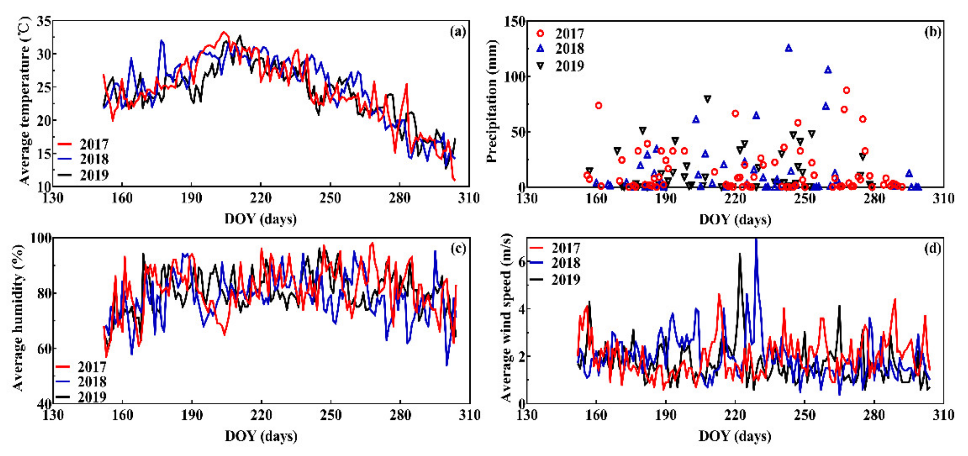
2.3. Meteorological Data Collection and Analysis

We collected meteorological data using the automated weather station Dynameta-1K (Dynamax Inc., Houston, TX, USA) from May to October (Figure 1), which included daily average temperature (Tem_daily) (°C), average relative humidity (%), accumulative precipitation (mm) and average wind speed (m/s). The temperature data was divided into Tem_daily and accumulated growing degree day (AGDD). AGDD represents the sum of growing degree days (GDD) from transplanting to test day, GDD = Tem_daily −12.5 °C [50].

To determine the effect of meteorological factors on rice PKC, we used a linear mixed effects model and set rice PKC as a dependent variable, meteorological factors as fixed effects, and day as a random effect with a random intercept. To avoid collinearity and overfitting, meteorological factors were removed using a stepwise multiple linear regression (SMLR) until the variance inflation factor (VIF) of all meteorological factors was less than 3 [51]. The linear mixed effects analysis was performed with the “lme4” package [52] in the R language (R Core Team, 2018). We considered meteorological factors at p < 0.001 to have a statistically significant effect on rice PKC and selected them as important meteorological factors (Ifs). The standardized slope (b*) was used to determine the effect size of each meteorological factor.

2.4. Modeling and Validation of Potassium Nutrition

The workflow associated with our approach to identify a reliable remote sensing model for predicting rice PKC is shown in Figure 2. First, using normalized difference spectral index (NDSI) and correlation analysis, we selected two-band indices and correlation bands (CBs) based on three transformed spectra (reflectance spectra (R), first derivative spectra (FD) and reciprocal logarithm-transformed (log [1/R])). Next, we used the genetic algorithms partial least-squares (GA-PLS) (more details see below) and linear mixed effects model to select important bands (IBs) and important meteorological factors (IFs), respectively. Finally, we used spectral indices and machine learning (partial least-squares regression (PLSR) and random forest (RF)) to build K nutrition RS models and combined RS models and IFs to build new K nutrition models. Furthermore, we used a validation dataset to evaluate the performance of K nutrition models and divided all data into different datasets to test the stability and temporal transferability of K models and selected optimal K models according to simplicity and estimation accuracy.

To select important bands that contribute the most to the variability of rice PKC, we performed variable selection with the commonly used GA-PLS [53]. GA-PLS was implemented through the “plsVarSel” package [54] in the R language. To compare the ability of simple spectral indices and machine learning methods to detect variability in rice PKC, we did the following. First, we built simple linear regression models between rice PKC and spectral indices proposed by previous studies and this paper. The optimal spectral index was selected by root mean square error (RMSE), bias and relative root mean square error (RE). Meanwhile, a SMLR model was developed between rice PKC and the optimal spectral index and IFs. To avoid overfitting, two statistical parameters of the SMLR model (VIF and tolerance (TOL)) were set less than 3 and greater than 0.33, respectively [51]. We also employed machine learning (i.e., PLSR and RF), which selected IBs and IFs as input variables. PLSR was implemented through the “pls” package [55] in the R language. RF included two important tuning parameters: (1) the number of regression trees (ntree) and (2) the number of predictors tested at each node (mtry). The ntree was set to 1000 according to previous studies [37,56] and mtry was determined by the “randomForest” package [57] in the R language.

To build the rice PKC estimation models and test their performance, a total of 864 samples from three growing seasons (2017–2019) were randomly split into a calibration (2/3 of data, 576 samples) and validation (1/3 of data, 288 samples) dataset (

Table 2. Statistics of PKC (%) for all 6 sampling times (tillering, productive tiller critical stage (N-n), jointing, booting, heading, and filling stage) for experiments conducted in 2017, 2018, and 2019.

	Dataset	Number of Samples	Min	Max	Mean	STD	CV (%)
PKC (%)	2017	288	0.82	3.76	2.22	0.60	26.94
	2018	288	0.86	4.17	2.36	0.67	28.48
	2019	288	0.55	3.52	2.16	0.74	34.49
	Calibration dataset	576	0.55	4.17	2.25	0.68	30.20
	Validation dataset	288	0.55	4.00	2.24	0.68	30.32
	All	864	0.55	4.17	2.25	0.68	30.22

Note: STD and CV are standard deviation and coefficient of variation (STD/Mean), respectively.

). The coefficient of determination (R²), RMSE, bias, RE, and Akaike information criterion (AIC) [58] of all model types were calculated in R (R Core Team, 2018) and used to evaluate the prediction accuracy of these models.

3. Results

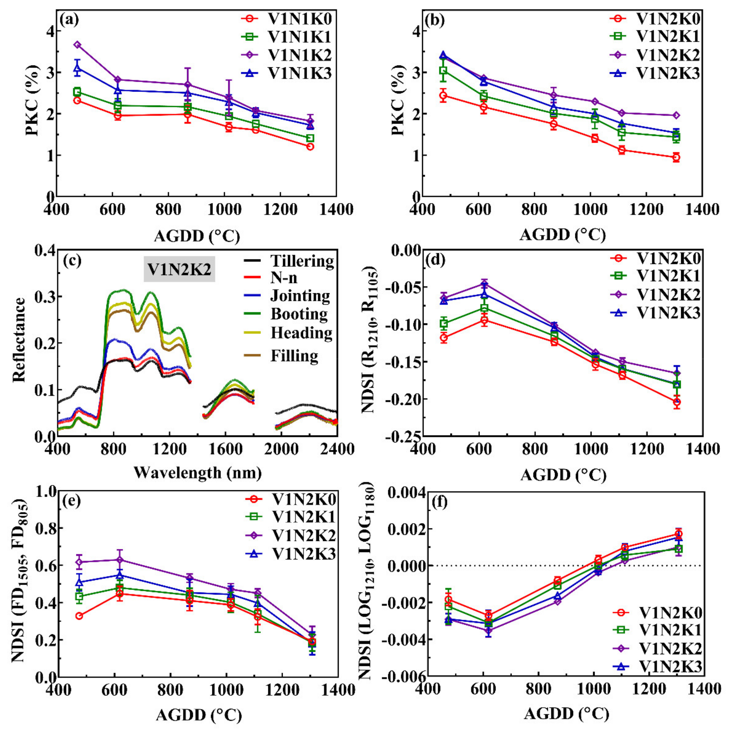
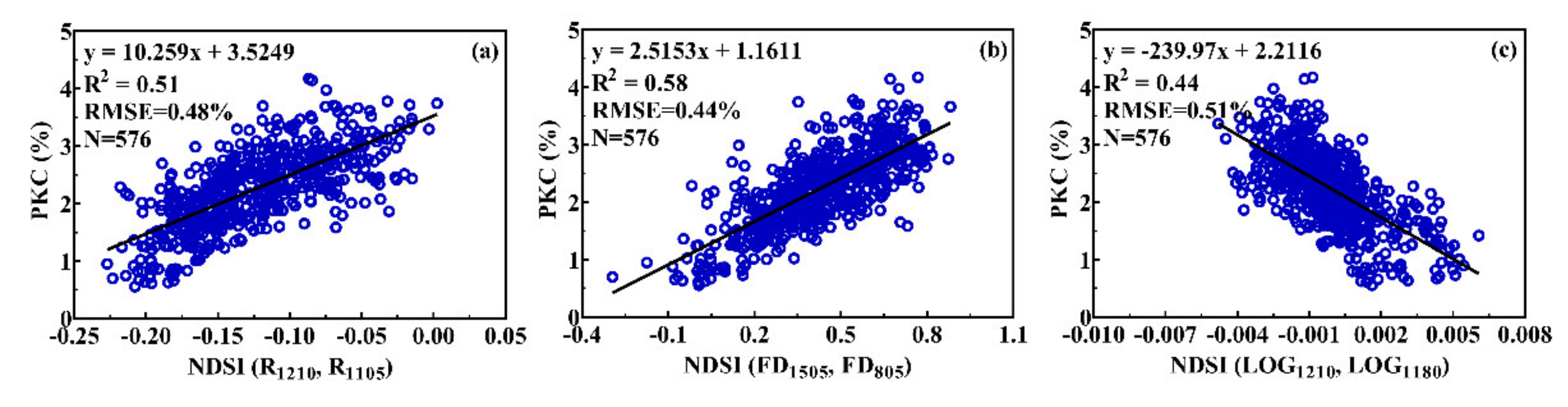
3.1. Variation Patterns of Rice PKC and Canopy Spectral Parameters

Table 2 showed the descriptive statistics of PKC for different datasets. The 2018 dataset exhibited a higher mean PKC, and the 2019 dataset exhibited a higher degree of dispersion. The PKC decreased with the growth of rice plant; the no K fertilization (K0) had the lowest PKC and K2 had the highest PKC (Figure 3a,b). We selected the optimal treatment (V1N2K2) to show the mean reflectance with six growth stages (Figure 3c); before the booting stage, the spectral reflectance decreased in the visible region and increased in the near-infrared region, after the booting stage, the spectral reflectance decreased in the near-infrared region due to the influence of ears. Then, we showed the variation pattern of mean NDSI for R, FD, and LOG with different AGDD (calculation of NDSI see Section 3.4), in summary, NDSI values of R and FD showed a similar variation, they decreased with the growth of rice plant, no K fertilization treatment (K0) had lowest NDSI value, and K2 had the high NDSI value (Figure 3d,e). For the NDSI value of LOG, it showed an opposite variation to R (Figure 3f).

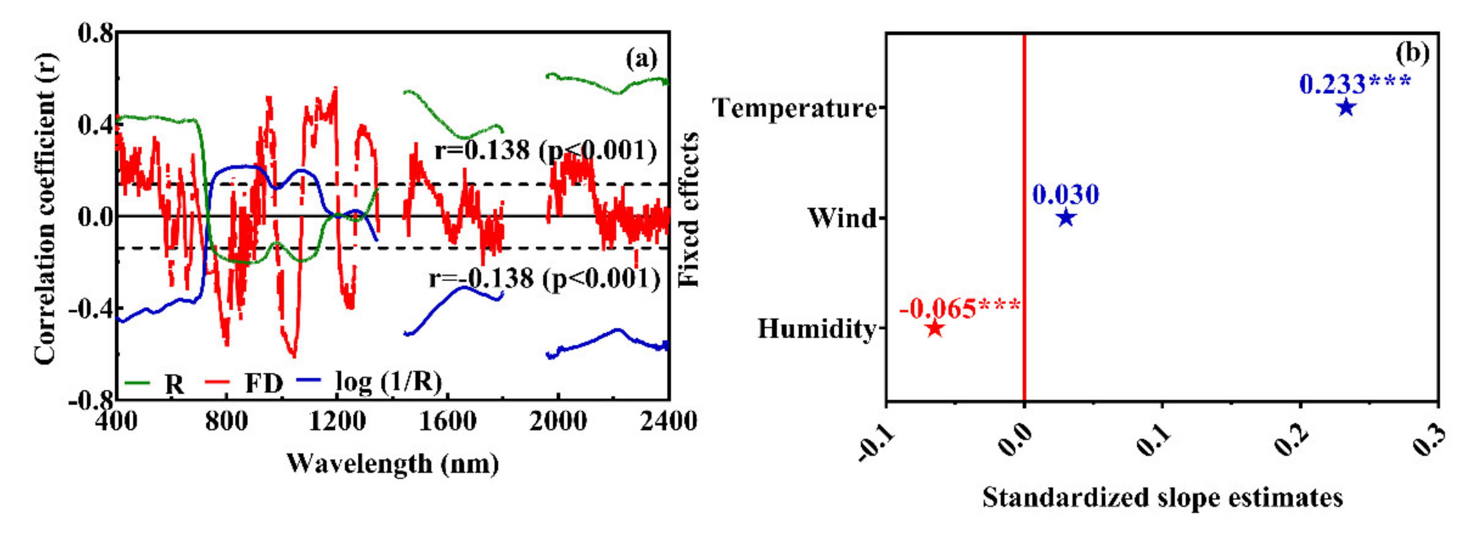
3.2. Correlation of Rice PKC with Spectral and Meteorological Data

The reflectance spectra (R) were positively correlated with rice PKC at 400–723, 1441–1800, and 1961–2400 nm (maximum R² value of 0.38 at 1969 nm) and negatively correlated at 750–955 and 1008–1130 nm (Figure 4a). The log (1/R) spectra had an opposite trend of the R spectra. The FD spectra had a negative correlation with rice PKC at 759–810, 985–1066, and 1268–1341 nm (maximum R² value of 0.38 at 1045 nm) and a positive correlation at 920–973 and 1077–1264 nm. Correlation bands (CBs) were selected by significant correlation analysis and used for selecting important bands (IBs) (see Section 3.3 below).

After excluding highly collinear meteorological factors based on TOL and VIF values (

Table 3. Results of stepwise multiple linear regression between meteorological data and rice plant potassium content.

Variables and Intercept	Value	R2 adj	p-Value	TOL	VIF
Intercept	−1.883	0.57	<0.001
Daily average temperature	0.221		<0.001	0.878	1.139
Daily average humidity	−0.031		<0.001	0.882	1.134
Daily average wind	0.170		<0.001	0.967	1.034

Note: VIF = variance inflation factor, TOL = tolerance, and R² adj = adjusted coefficient of determination.

), we fit a linear mixed effects model with daily average temperature, humidity, and wind speed as fixed effects and day as a random effect with a random intercept on rice PKC. The results from the linear mixed effects model revealed that daily average temperature had the strongest (b* = 0.233, p < 0.001) significant effect on the rice PKC, followed by average humidity (b* = −0.065, p < 0.001) (Figure 4b). Thus, daily average temperature and humidity were selected as important meteorological factors (Ifs).

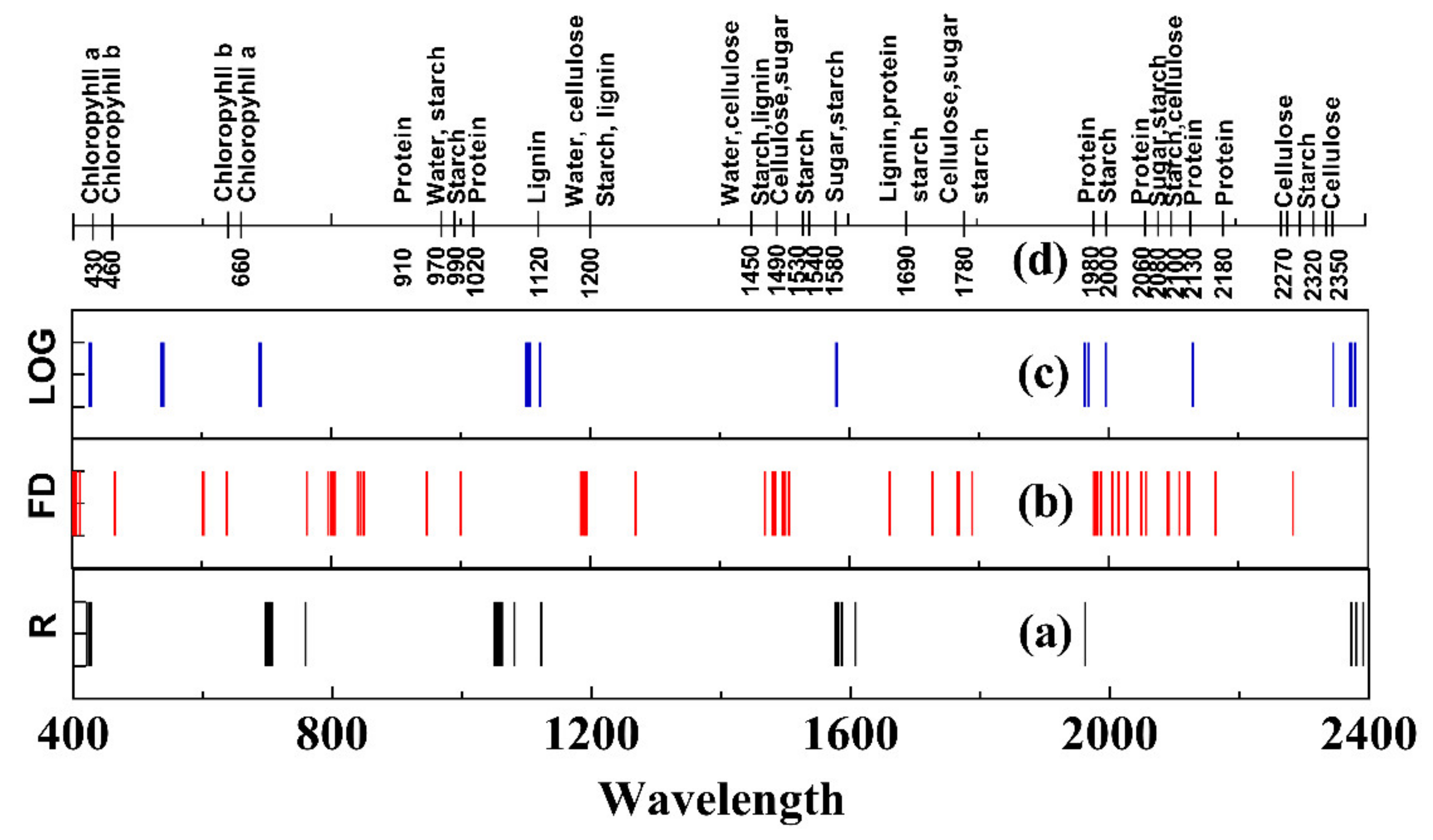
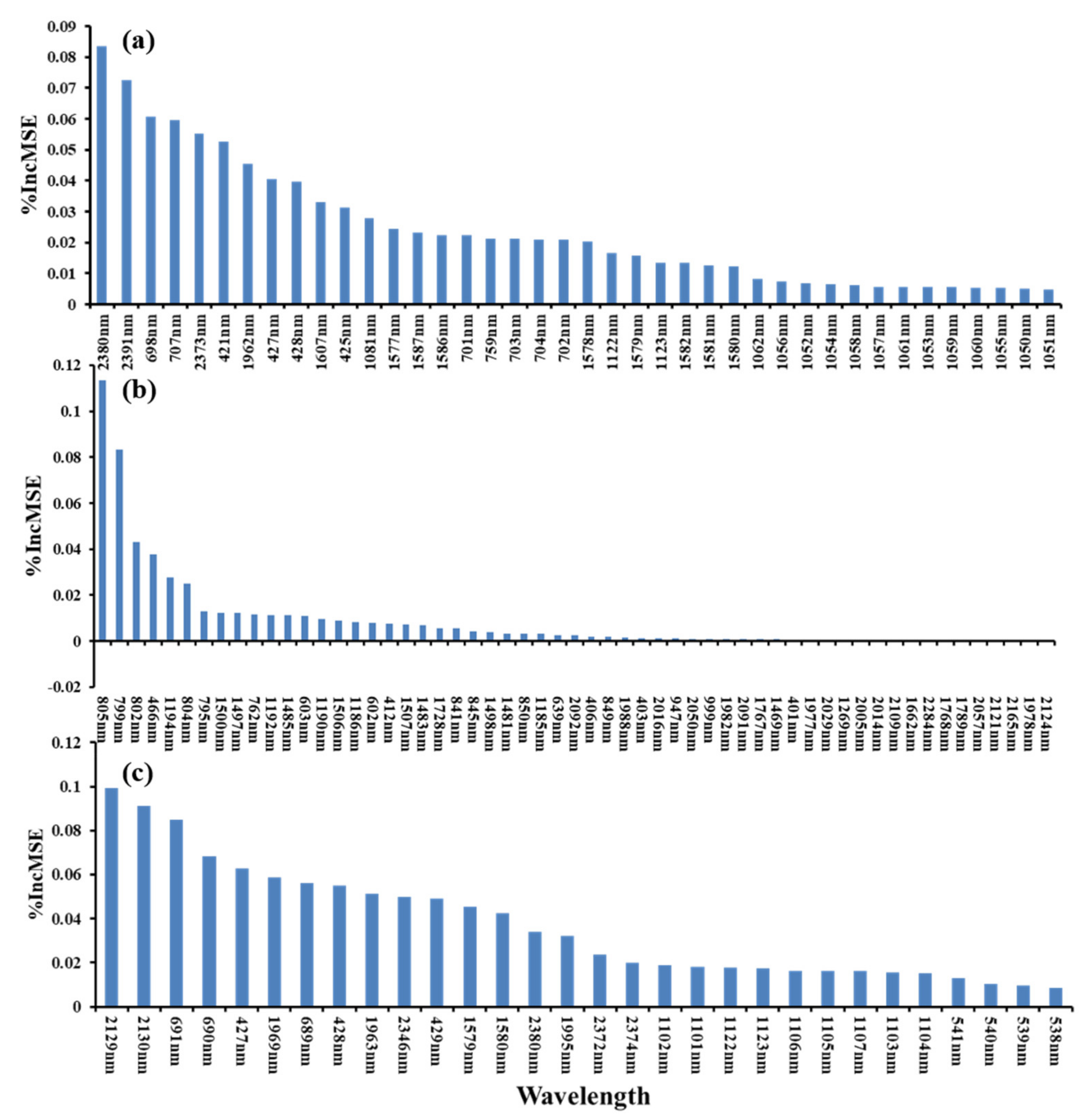
3.3. Important Bands Selection

The GA-PLS was used to select IBs that were sensitive to variability in rice PKC from the CBs. The results showed that the number of IBs were 40, 57, and 30 for the R, FD, and Log (1/R), respectively (

Table 4. Correlation bands and important bands selection using correlation analysis and GA-PLS, respectively.

Variables	CBs	Numbers of CBs	IBs	Numbers of IBs
R	400–723; 750–955; 1008–1130; 1441–1800; 1961–2400 nm	1453	421; 425; 427–428; 698; 701–704; 707; 759; 1050–1062; 1081; 1122–1123; 1577–1582; 1586–1587; 1607; 1962; 2373; 2380; 2391 nm	40
FD	400–420 … 713–715; 717–757; 759–810; 920–973…… 985–1066; 1077–1264; 1268–1341 … 1465–1473; 1477–1531; 1728–1730 … 1976–1978; 2014–2018; 2027–2033 … 2071–2078; 2090–2095; 2281–2284 nm	918	401; 403; 406; 412; 466; 602–603; 639; 762; 795; 799; 802; 804–805; 841; 845; 849–850; 947; 999; 1185–1186; 1190; 1192; 1194; 1269; 1469; 1481; 1483; 1485; 1497–1498; 1500; 1506–1507; 1662; 1728; 1767–1768; 1789; 1977–1978; 1982; 1988; 2005; 2014; 2016; 2029; 2050; 2057; 2091–2092; 2109; 2121; 2124; 2165; 2284 nm	57
Log (1/R)	400–724; 747–957; 1004–1130; 1441–1800; 1961–2400 nm	1463	427–429; 538–541; 689–691; 1101–1107; 1122–1123; 1579–1580; 1963; 1969; 1995; 2129–2130; 2346; 2372; 2374; 2380 nm	30

Note: R = reflectance, FD = first derivative spectra, Log (1/R) = reciprocal logarithm-transformed spectra, CBs = correlation bands, IBs = important bands, and GA-PLS = genetic algorithms partial least-squares.

). Some IBs for transformed spectra were located in the visible region that was influenced by pigment content. Most IBs for transformed spectra were located in near-infrared and shortwave infrared regions that were influenced by water, protein, starch, lignin, cellulose, and sugar (Figure 5d).

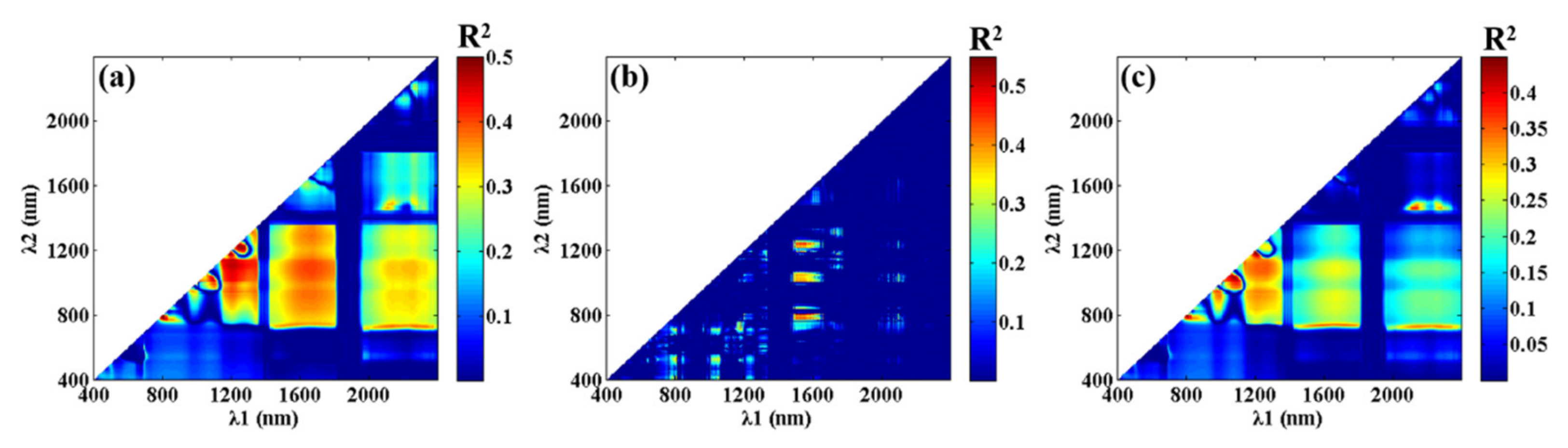
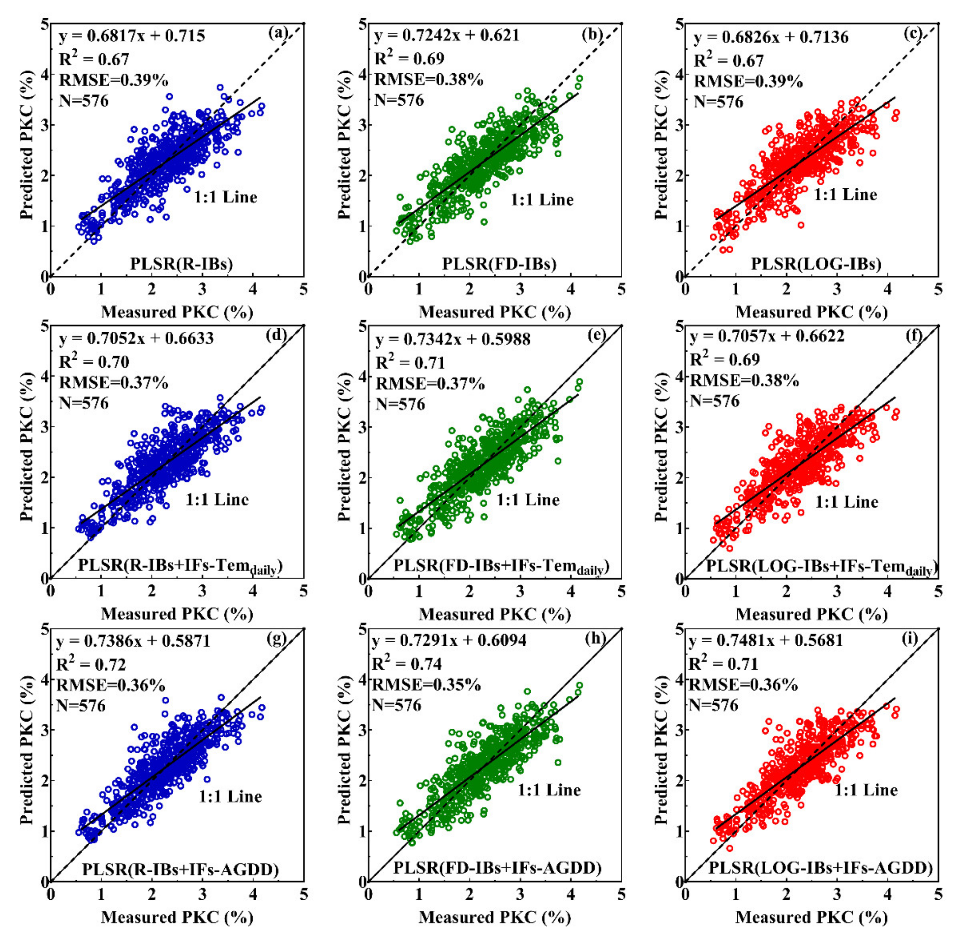
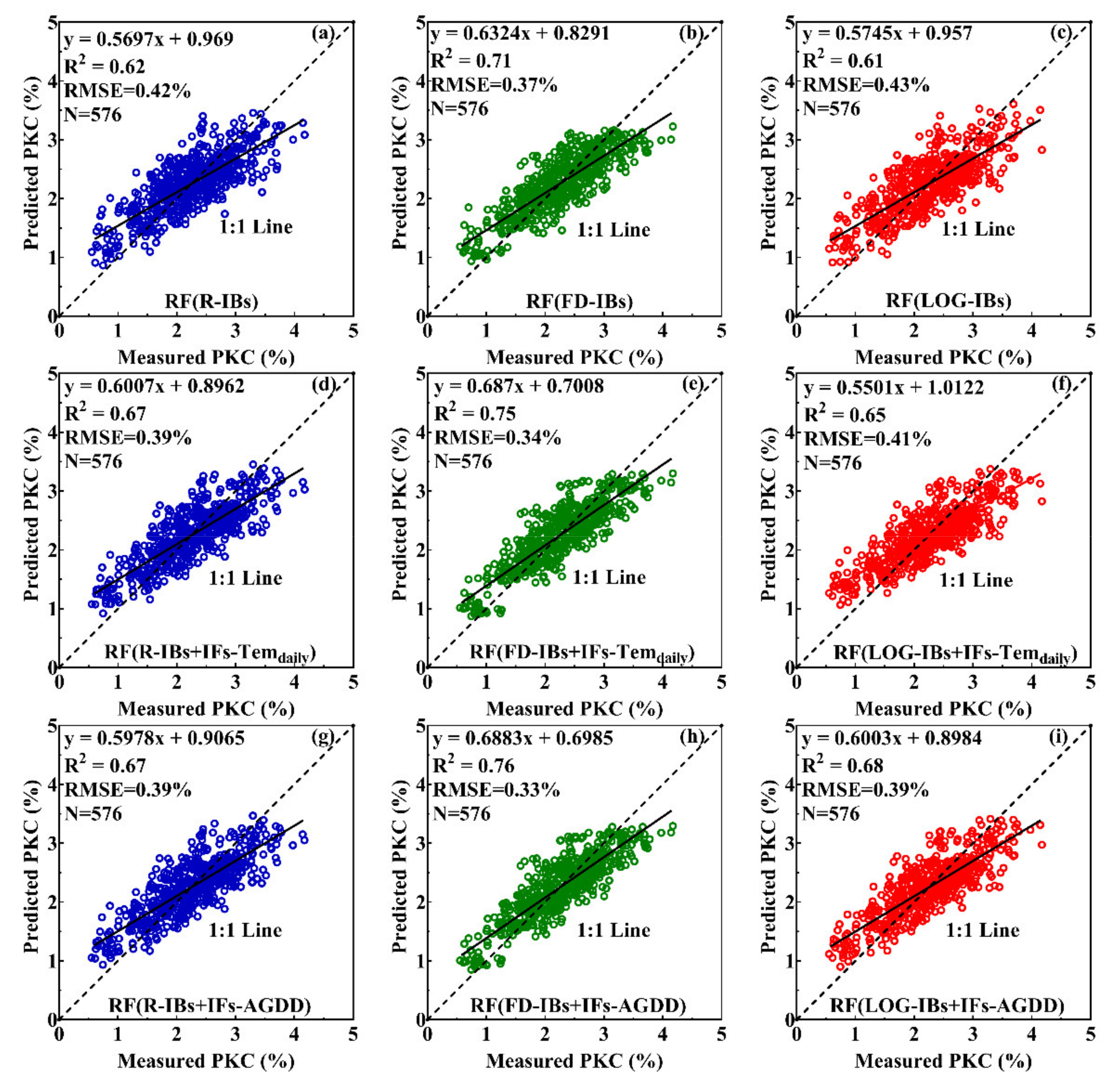
3.4. Estimation of Rice PKC with Spectral Index and Machine Learning Methods

For this part of the analysis, we selected two RS methods (spectral index and machine learning) to compare their ability to detect variations in rice PKC. A random combination with two bands of different transformed spectra was selected to construct a normalized spectral index (NDSI) (Figure 6) following previous work [9]. Our results showed NDSI (R₁₂₁₀, R₁₁₀₅), NDSI (FD₁₅₀₅, FD₈₀₅), and NDSI (LOG₁₂₁₀, LOG₁₁₈₀) to be the strongest predictors of rice PKC among the spectral indices based on R (R² = 0.51, RMSE = 0.48%), FD (R² = 0.58, RMSE = 0.44%), and log (1/R) spectra (R² = 0.44, RMSE = 0.51%) (Figure 7). Additionally, among previously identified spectral indices (see

Table 5. Relationship between rice plant potassium content (PKC) and new spectral indices and existing spectral indices using the calibration dataset.

Spectral Indices	Calibration	Validation
	R2	R2	RMSE (%)	RE (%)	Bias (%)
NDSI (FD1505, FD805) *	0.58	0.53	0.47	20.70	0.008
NDSI (R1210, R1105) *	0.51	0.47	0.49	22.00	0.011
NDSI(LOG1210, LOG1180) *	0.44	0.44	0.51	22.72	0.007
NDSI (R1645, R1715)	0.39	0.35	0.55	24.45	0.018
NDSI (R1705, R1320)	0.32	0.29	0.57	25.49	0.011
NDSI (R870, R1450)	0.21	0.15	0.63	27.90	0.014
NDSI (R523, R583)	0.01	0.02	0.67	29.97	0.010
FD1686	0.03	0.01	0.68	30.43	0.008
R780/R650	0.02	0.00	0.68	30.24	0.007
Log(1/R1337)	0.01	0.01	0.68	30.14	0.010
NDSI (FD1450, FD1295)	0.02	0.05	0.69	30.97	0.001
FD760/FD630	0.01	0.12	0.72	32.04	0.024

Note: R = reflectance, FD = first derivative spectra, and LOG = reciprocal logarithm-transformed spectra. We use the reflectance at 1320 nm and 1450 nm to replace at 1385 nm and 1430 nm due to the influence of atmospheric moisture absorption at 1385 nm at the canopy level. * represents spectral indices proposed in this paper.

), NDSI (R₁₆₄₅, R₁₇₁₅) (R² = 0.39, RMSE = 0.55%), NDSI (R₁₇₀₅, R₁₃₂₀) (R² = 0.32, RMSE = 0.57%) and NDSI (R₈₇₀, R₁₄₅₀) (R² = 0.21, RMSE = 0.63) showed to be the strongest predictors of rice PKC. R₇₈₀/R₆₅₀, NDSI (R₅₂₃, R₅₈₃), FD₇₆₀/FD₆₃₀, FD₁₆₈₆, NDSI (FD₁₄₅₀, FD₁₂₉₅), and Log(1/R₁₃₃₇) showed to be the poorest predictors of rice PKC (R² < 0.05, RMSE > 0.67%) (Table 5).

For our machine learning models (PLSR and RF), we used IBs identified with GA-PLS to predict rice PKC. The PLSR model based on FD-IBs showed to be the strongest predictor of rice PKC (R² = 0.69, RMSE = 0.38%) (Figure 8b), followed by the PLSR models based on R-IBs and LOG-IBs (R² = 0.67, RMSE = 0.39%) (Figure 8a,c). RF modelling showed similar results to PLSR modelling and the RF model based on FD spectra showed to be the strongest predictor of rice PKC, followed by RF models based on R-IBs and LOG-IBs (R² = 0.71, 0.62 and 0.61, RMSE = 0.37%, 0.42% and 0.43%, respectively) (Figure 9a–c). Compared to the ability of spectral indices to detect the variations in rice PKC, the machine learning methods showed better estimation accuracy (R² and RMSE increase and decrease of more than 0.1 and 0.06%, respectively).

3.5. Estimation of Rice PKC with a Combination of Remote Sensing and Meteorological Data

Here, we added meteorological data identified in our correlation analyses (see Section 3.2) into RS models. The optimal spectral indices among different transformed spectra and IFs (daily average temperature and humidity) were selected to develop SMLR models (

Table 6. Results of stepwise multiple linear regression with spectral indices and meteorological data using the calibration dataset.

Transformed Spectra	Variables and Intercept	Value	R2 adj	p-Value	TOL	VIF
R	Intercept	−1.194	0.60	<0.001
	NDSI (R1210, R1105)	0.145		<0.001	0.441	2.269
	Average temperature	5.413		<0.001	0.441	2.269
FD	Intercept	−1.811	0.64	<0.001
	NDSI (FD1505, FD805)	1.606		<0.001	0.441	2.268
	Average temperature	0.118		<0.001	0.441	2.268
LOG	Intercept	−1.638	0.58	<0.001
	NDSI (LOG1210, LOG1180)	0.217		<0.001	0.890	1.124
	Average temperature	−0.028		<0.001	0.890	1.124
R	Intercept	3.991	0.65	<0.001
	AGDD	−0.002		<0.001	0.335	2.988
	NDSI (R1210, R1105)	2.152		<0.001	0.335	2.988
FD	Intercept	2.927	0.68	<0.001
	AGDD	−0.001		<0.001	0.37	2.704
	NDSI (FD1505, FD805)	1.117		<0.001	0.37	2.704
LOG	Intercept	4.736	0.64	<0.001
	AGDD	−0.002		<0.001	0.347	2.879
	Humidity	−0.012		<0.001	0.826	1.211
	NDSI (LOG1210, LOG1180)	−31.414		<0.001	0.374	2.675

Note: R = reflectance, FD = first derivative spectra, LOG = reciprocal logarithm-transformed spectra, AGDD = accumulated growing degree day, VIF = variance inflation factor, TOL = tolerance, and R² adj = adjusted coefficient of determination.

). We found that SMLR models that combined spectral indices and IFs improved the estimation accuracy of rice PKC, and the model based on the FD index performed better than R and log (1/R) indices for estimating rice PKC. The SMLR model of NDSI (FD₁₅₀₅, FD₈₀₅) + AGDD showed the best performance for estimating rice PKC, followed by NDSI (R₁₂₁₀, R₁₁₀₅) + AGDD and NDSI (LOG₁₂₁₀, LOG₁₁₈₀) + AGDD. Compared to the models using spectral index alone, the R² of these SMLR models increased by 17.24%, 24.45%, and 45.45% to 0.68, 0.65, and 0.64, respectively.

The IBs (Table 4) and IFs were used as independent variables of machine learning methods to build models with rice PKC. The PLSR models using FD-IBs and IFs resulted in the most accurate rice PKC estimates (R² = 0.71, 0.74, RMSE = 0.37%, 0.35%, respectively) (Figure 8e,h), followed by PLSR models based on R-IBs + Ifs and LOG-Ibs + Ifs, respectively (Figure 8d,f,g,i). The RF models based on FD-Ibs + Ifs showed to most accurately predict variability in rice PKC (R² = 0.75 and 0.76, RMSE = 0.34%, 0.33%, respectively) (Figure 9e,h), followed by RF models based on R-Ibs + Ifs (R² = 0.67, RMSE = 0.39%, respectively) (Figure 9d,g) and LOG-Ibs + Ifs (R² = 0.65, 0.68, RMSE = 0.41%, 0.39%, respectively) (Figure 9f,i). Compared to the machine learning models using Ibs alone, the models using a combination of Ibs and Ifs could slightly improve the estimation precision of rice PKC (R² increased by 5.97–11.47%).

3.6. Model Evaluation and Testing

We used a validation dataset to evaluate the performance of rice PKC models (

Table 7. Relationships of plant potassium content (PKC) and various methods.

Type of Modeling	Methods	Calibration	Validation
		R2	R2	RMSE (%)	RE (%)	Bias (%)	AIC
LR (Section 3.4)	NDSI (R1210, R1105)	0.51	0.47	0.49	22.00	0.011	−401
SMLR (Section 3.5)	NDSI(R1210,R1105) + Temdaily	0.60	0.55	0.45	20.20	0.002	−447
SMLR (Section 3.5)	NDSI (R1210, R1105) + AGDD	0.65	0.61	0.42	18.92	−0.004	−486
LR (Section 3.4)	NDSI(FD1505, FD805)	0.58	0.53	0.47	20.70	0.008	−436
SMLR (Section 3.5)	NDSI (FD1505, FD805) + Temdaily	0.64	0.59	0.43	19.30	0.002	−475
SMLR (Section 3.5)	NDSI(FD1505, FD805) +AGDD	0.68	0.63	0.41	18.36	0.001	−504
LR (Section 3.4)	NDSI(LOG1210, LOG1180)	0.44	0.44	0.51	22.72	0.007	−383
SMLR (Section 3.5)	NDSI(LOG1210, LOG1180) + Temdaily	0.58	0.55	0.46	20.32	0.008	−445
SMLR (Section 3.5)	NDSI(LOG1210, LOG1180) +AGDD	0.64	0.62	0.42	18.78	−0.001	−491
PLSR (Section 3.4)	PLSR(R-IBs)	0.67	0.64	0.41	18.14	0.007	−438
PLSR (Section 3.5)	PLSR(R-IBs + IFs-Temdaily)	0.70	0.67	0.39	17.50	0.009	−455
PLSR (Section 3.5)	PLSR(R-IBs + IFs-AGDD)	0.72	0.69	0.38	17.08	−0.200	−486
PLSR (Section 3.4)	PLSR(FD-IBs)	0.69	0.71	0.37	16.56	−0.012	−485
PLSR (Section 3.5)	PLSR(FD-IBs + IFs-Temdaily)	0.71	0.71	0.36	16.30	−0.015	−501
PLSR (Section 3.5)	PLSR(FD-IBs + IFs-AGDD)	0.74	0.73	0.35	15.88	0.014	−524
PLSR (Section 3.4)	PLSR(LOG-IBs)	0.67	0.67	0.39	17.42	−0.006	−440
PLSR (Section 3.5)	PLSR(LOG-IBs + IFs-Temdaily)	0.69	0.69	0.38	16.96	−0.006	−447
PLSR (Section 3.5)	PLSR(LOG-IBs + IFs-AGDD)	0.72	0.70	0.37	16.54	−0.015	−455
RF (Section 3.4)	RF(R-IBs)	0.62	0.56	0.47	21.26	0.160	−347
RF (Section 3.5)	RF(R-IBs + IFs-Temdaily)	0.67	0.63	0.45	20.24	0.180	−371
RF (Section 3.5)	RF(R-IBs + IFs-AGDD)	0.67	0.63	0.45	20.15	0.179	−374
RF (Section 3.4)	RF(FD-IBs)	0.71	0.70	0.40	17.96	0.130	−445
RF (Section 3.5)	RF(FD-IBs + IFs-Temdaily)	0.75	0.75	0.37	16.60	0.120	−488
RF (Section 3.5)	RF(FD-IBs + IFs-AGDD)	0.76	0.75	0.37	16.69	0.128	−493
RF (Section 3.4)	RF(LOG-IBs)	0.61	0.57	0.44	19.78	0.019	−388
RF (Section 3.5)	RF(LOG-IBs + IFs-Temdaily)	0.65	0.63	0.43	19.02	0.046	−423
RF (Section 3.5)	RF(LOG-IBs + IFs-AGDD)	0.68	0.66	0.40	18.06	0.039	−432

Note: R = reflectance, FD = first derivative spectra, LOG = reciprocal logarithm-transformed spectra, IBs = important bands, IFs = important meteorological factors, NDSI = normalized difference spectral index, LR = linear regression, SMLR = stepwise multiple linear regression, PLSR = partial least-squares regression, RF = random forest, AGDD = accumulated growing degree day, IFs-Tem_daily represents daily average temperature and humidity, IFs-AGDD represents AGDD and daily average humidity, and the italic font represents the best performances of various methods.

) and the results showed that NDSI (FD₁₅₀₅, FD₈₀₅) had a best performance for predicting rice PKC (RMSE = 0.47%, RE = 20.70%, bias = 0.008%, AIC = −436), followed by NDSI (R₁₂₁₀, R₁₁₀₅) and NDSI (LOG₁₂₁₀, LOG₁₁₈₀), respectively. The models of spectral index + AGDD showed higher prediction accuracies than spectral index + Tem_daily and NDSI (FD₁₅₀₅, FD₈₀₅) + AGDD showed a best performance for predicting rice PKC (RMSE = 0.41%, RE = 18.36%, bias = 0.001%, AIC = −504), followed by NDSI (R₁₂₁₀, R₁₁₀₅) + AGDD and NDSI (LOG₁₂₁₀, LOG₁₁₈₀) + AGDD, respectively. Compared to the PKC models using spectral index alone, the models using spectral index + AGDD had smaller RMSE, RE, and bias values.

The models based on machine learning approaches showed higher prediction accuracies of rice PKC than spectral indices and had smaller RMSE and RE values. The PLSR (FD-IBs) models showed the best prediction accuracies of rice PKC (RMSE = 0.37%, RE = 16.56%, bias = −0.012%, AIC = −485), followed by PLSR (LOG-IBs) and PLSR (R-IBs), respectively. The PLSR models using IBs + IFs-AGDD showed higher prediction accuracies than those using IBs + IFs-Tem_daily and PLSR (FD-IBs + IFs-AGDD) showed the best prediction accuracies of rice PKC (RMSE = 0.35%, RE = 15.88%, bias = 0.014%, AIC = −524), followed by PLSR (LOG-IBs + IFs-AGDD) and PLSR (R-IBs + IFs-AGDD), respectively. The RF (FD-IBs) models had the best performance for predicting rice PKC (RMSE = 0.40%, RE = 17.96%, bias = 0.130%, AIC = 445), followed by RF (LOG-IBs) and RF (R-IBs), respectively. The RF (IBs + IFs-AGDD) models showed higher prediction accuracies than RF (IBs + IFs-Tem_daily) models and RF (FD-IBs + IFs-AGDD) showed a best performance for predicting rice PKC, followed by RF (LOG-IBs + IFs) and RF (R-IBs + IFs), respectively. Compared to the models of machine learning using IBs alone, the models using IBs + IFs showed better performance and had smaller RMSE and RE values.

To test the stability and temporal transferability of rice PKC models further, all the data was divided into eleven different datasets according to N level, K level, variety, and experiment year (

Table 8. Correlations between rice plant potassium content (PKC) and different remote sensing methods under the different datasets.

Methods		Variety		Nitrogen		Potassium				Experiments (Exp.)
		Japonica	Indica	N1	N2	K0	K1	K2	K3	Exp.1	Exp.2	Exp.3
NDSI (R1210, R1105)	R2	0.51	0.53	0.59	0.46	0.64	0.65	0.56	0.65	0.44	0.57	0.46
	RMSE (%)	0.49	0.44	0.41	0.53	0.33	0.37	0.45	0.40	0.45	0.44	0.55
NDSI (R1210, R1105) + AGDD	R2	0.67	0.55	0.68	0.61	0.69	0.78	0.72	0.78	0.61	0.68	0.72
	RMSE (%)	0.40	0.43	0.38	0.47	0.30	0.29	0.36	0.31	0.37	0.38	0.39
NDSI (FD1505, FD805)	R2	0.57	0.56	0.60	0.55	0.64	0.71	0.55	0.68	0.43	0.58	0.66
	RMSE (%)	0.46	0.43	0.41	0.48	0.32	0.34	0.45	0.38	0.45	0.44	0.44
NDSI (FD1505, FD805) +AGDD	R2	0.72	0.62	0.73	0.62	0.73	0.82	0.72	0.80	0.62	0.71	0.73
	RMSE (%)	0.38	0.40	0.33	0.44	0.28	0.27	0.36	0.30	0.37	0.36	0.39
PLSR (FD-IBs)	R2	0.69	0.62	0.73	0.65	0.73	0.80	0.76	0.78	0.61	0.76	0.76
	RMSE (%)	0.39	0.40	0.36	0.42	0.28	0.29	0.34	0.31	0.37	0.33	0.36
PLSR (FD-IBs + IFs-AGDD)	R2	0.71	0.70	0.80	0.65	0.76	0.83	0.79	0.82	0.63	0.76	0.78
	RMSE (%)	0.38	0.35	0.29	0.42	0.26	0.26	0.32	0.28	0.36	0.33	0.34
RF (FD-IBs)	R2	0.74	0.62	0.75	0.69	0.79	0.82	0.74	0.81	0.64	0.75	0.78
	RMSE (%)	0.34	0.40	0.33	0.40	0.24	0.27	0.35	0.29	0.36	0.34	0.34
RF (FD-IBs + IFs-AGDD)	R2	0.78	0.75	0.82	0.71	0.83	0.88	0.82	0.87	0.67	0.78	0.81
	RMSE (%)	0.33	0.33	0.27	0.39	0.22	0.22	0.30	0.24	0.34	0.32	0.32

Note: R = reflectance, FD = first derivative spectra, IBs = important bands, IFs = important meteorological factors, NDSI = normalized difference spectral index, PLSR = partial least-squares regression, RF = random forest, AGDD = accumulated growing degree day, and IFs-AGDD represents AGDD and daily average humidity.

). We selected NDSI (R₁₂₁₀, R₁₁₀₅) and NDSI (FD₁₅₀₅, FD₈₀₅) using fewer bands and PLSR (FD-IBs) and RF (FD-IBs) using many bands to test their performance. Our results showed that the rice PKC models of spectra combined with meteorological factors could better detect the variability of rice PKC than using spectra alone (with higher R² and lower RMSE). Considering the ability of RS models for detecting the variability in rice PKC, they performed better when used in japonica rice than indica rice; Low N level (N1) could be better detected by them than high N level (N2); K stress levels could be better detected by them than normal K level: K1 > K3 > K0 > K2. Meanwhile, the K RS models have good performances under different years and performed better when used in Exp. 3 (2019) than Exp. 2 (2018) and Exp. 1 (2017). Finally, we selected the optimal PKC models: one was NDSI (FD₁₅₀₅, FD₈₀₅) + AGDD; another was PLSR (FD-IBs + IFs) and RF (FD-IBs + IFs).

4. Discussion

4.1. Canopy Sensitive Bands and Transformed Spectra for Plant K Estimation

Our results showed that the spectral bands of rice canopy that were sensitive to PKC were mainly concentrated in the near-infrared and shortwave infrared regions (1000–1340 nm, 1450–1800 nm, and 1961–2400 nm) (Figure 6a). This result was consistent with previous studies that the shortwave infrared spectra could be used to identify crop K nutrition levels in other crops [9,15,62,63]. The K spectral index proposed here included bands at 1210 nm and 1505 nm (Table 5), which have previously been used to construct a spectral index to monitor vegetation moisture status [64]. Meanwhile, the K spectral indices NDSI (R₁₆₄₅, R₁₇₁₅) and NDSI (R₈₇₀, R₁₄₅₀) proposed by Pimstein et al. [15] and NDSI (R₁₇₀₅, R₁₃₂₀) proposed by Lu et al. [9] performed well in this paper, included shortwave infrared bands and these bands were also closely related to vegetation moisture status [65]. In addition, most of the important bands selected by GA-PLS were also located in the near-infrared and shortwave infrared regions, and only a few important bands were located in visible regions (Figure 5). The near-infrared and shortwave infrared bands contributed the most to the K estimation (Figure 10). For K element, it does not have strong absorption features in spectra, and their predictions are due in part to correlations with other traits such as pigments, water, starch, protein, cellulose, and sugar [66,67]. One physiological explanation of why important spectral regions for the remote sensing of K appear to be mainly located in the near-infrared and shortwave infrared spectral regions is that K exists in the form of K ions in the plant, which regulates stomatal conductance and osmotic potential, and enhances the synthesis of many enzymes, proteins, starches, and cellulose [1]. Finally, the variations in the plant K element will influence the spectral changes of corresponding absorption features.

The rice PKC models using a novel spectral index and machine learning based on the FD spectra showed better estimation accuracy than these rice PKC models based on the R spectra (Table 7). This was consistent with the conclusion by Lu et al. [9] who found that the FD spectral index was better than the R spectral index on estimating the rice leaf K content, and Gao et al. [47] found that the performance of machine learning based on the FD spectra on estimating leaf phosphorus content in forage was better than the R spectra. The K RS models using FD spectra had a better performance than using the original reflectance spectra in that FD spectra could reduce noise signals generated by atmospheric water absorption, soil background, and data redundancy, and enhance the absorption characteristics of plant leaf biochemical parameters [23].

4.2. Performance of Spectral Index and Machine Learning for Estimating Plant K

The results of this paper showed that the optimal estimation model of rice PKC could be divided into two types: one was the spectral index NDSI (FD₁₅₀₅, FD₈₀₅) using two bands, and the R² and RMSE of the model were 0.58 and 0.47%, respectively. Another was the PLSR (FD-IBs) and RF (FD-IBs) of the machine learning method using multi-band spectral information, the R² of the models were 0.69 and 0.71, and the RMSEs were 0.37% and 0.40%, respectively. The spectral index-based approach requires only two bands, hence it seems to be feasible to design a relatively low-cost sensor that could be installed on a tractor or Unmanned Aerial Vehicle to inform K fertilizer decisions. Even though the estimation accuracy was higher for machine learning approaches, they rely on data from hyperspectral sensors that are expensive, fragile, and require expert knowledge to be processed. Hence, for K nutrition estimation, machine learning approaches might be most useful for scientists, but might be less practical for operational decision making.

4.3. Incorporating Remote Sensing and Meteorological Data for Plant K Estimation

Of the meteorological variables in our study, the daily average temperature contributed the most to estimating rice PKC (b* = 0.233), followed by the daily average humidity (b* = −0.065). This was consistent with previous studies [39,40,42] that found rising temperature would increase crop K uptake. Similarly, Gisleröd et al. [68] showed that reducing air humidity would increase plant K uptake. Meanwhile, Yin et al. [41] also found an increase in average temperature and evaporation would increase the demand for potash fertilizer. The increase or decrease in average temperature and humidity will affect stomata opening and closing, thereby influencing plant transpiration and water transfer. K is closely related to water [9], which mainly regulated the opening and closing of stomata and the penetration potential to affect plant moisture status [69]. Thus, the daily average temperature and humidity will affect crop K uptake. Our study suggested that combining RS and meteorological data could effectively improve the estimation accuracy of crop K nutrition. Specifically, combining spectral and IFs-AGDD in models outperformed models with spectral and IFs-Tem_daily (Table 7). AGDD represents the effective accumulated temperature that crops require to complete their different growth stages [70], which suggests the accumulated temperature is more important than daily conditions for our results. Our finding that meteorological information could improve the RS of rice PKC in all model types was consistent with previous works which found that combining spectra and meteorological factors could improve the estimation accuracy of forage P content [47,49]. Similarly, other studies found that combining spectra and meteorological factors could improve the estimation accuracy of crop yield [33,46,48,71]. Meteorological factors mainly represent plant environmental information that plants are dynamically responding to and the spectra represent the current status of the plant. This might explain why combining spectra and meteorological factors can improve the accuracy of crop K nutrition estimation.

4.4. Evaluation of K Models and Future Directions

Compared to K estimation models using remote sensing data alone, the optimal K estimation models proposed in this study which incorporated meteorological data showed better stability under different datasets and better temporal transferability between different years (Table 8). The reason why RS models performed better when used in japonica rice than in indica rice is that japonica rice is more sensitive to K, which leads to more abundant K accumulation [9,19]. Low N levels can be better detected using RS than high N levels due to ammonium ions in plant roots under high N concentrations, which have an inhibitory effect on K uptake and thus reduce plant K accumulation [72]. K stress levels can be better detected using RS than normal K levels, indicating that K stress could affect the stomatal opening and closing of plant leaves and osmotic potential regulation, thus affecting leaf water status [73]. Therefore, vegetation signals under K stress are easier to remotely sense. Though beyond the scope of this study, phosphorus levels may also influence the transfer of soil potassium ions. Therefore, it would be valuable if future work could focus on the interaction between phosphorus and potassium.

When we tested the performance of RS models in different years, our result showed that RS models performed better when used in Exp. 3 (2019) than Exp. 2 (2018) and Exp. 1 (2017); this is as our study carried out the same K treatment experiment of a rice–wheat rotation system in the same experiment location. With the progress of the experiment, the difference of soil K gradient is more obvious, which can be seen from the coefficient of variation of the dataset (Table 2). Hence, the K gradient difference of Exp. 3 is the largest and the estimation accuracy of the K nutrition model is the highest. These experiments were conducted at only one crop and ecological site and the band used in the novel K spectral indices had been used for monitoring vegetation water status. Additionally, for other crops at different field sites, variability in topography will likely influence water movement and hence the availability of K. Thus, future studies should consider the topography attributes as predictor variables and test their importance in different crops, field sites (including different soil types), and drought stress conditions. Meanwhile, the ease of access to meteorological data continues to increase thanks to the establishment of environmental monitoring networks in many agricultural regions [74], fusing NDSI from a multi-band remote sensing device with air temperature and humidity information from the environmental monitoring networks could help to more effectively manage PKC in rice.

5. Conclusions

This study systematically compared the performance of different transformed spectra, spectral indices, machine learning, and spectra combined with meteorological factors for estimating rice K nutrition. Results showed that the K sensitive bands for rice canopy were mainly located in the near-infrared and shortwave infrared regions of the electromagnetic spectrum. The K nutrition models of spectral index and machine learning based on the FD spectra showed good estimation accuracy. Meanwhile, among the meteorological factors, daily average temperature explained most of the variability of observed rice PKC, followed by daily average humidity. The estimation accuracy of rice PKC could be significantly improved by combining spectra and meteorological data in all model types. The rice PKC estimation models of NDSI (FD1505, FD805) + AGDD, PLSR (FD-IBs + IFs-AGDD) and RF (FD-IBs + IFs-AGDD) showed the best performance, with R² of 0.68, 0.74, and 0.76, and RMSEs of 0.41, 0.35, and 0.37, respectively. Furthermore, the optimal models showed better stability and temporal transferability under different years and cultivation factors (N and K levels and varieties). Our findings will provide novel evidence for the improved estimation of crop K nutrition based on RS combined with meteorological data.

References

1. Marschner, P. Marschner’s Mineral Nutrition of Higher Plants, 3rd ed.; Academic Press: London, UK, 2012; pp. 1–3. [Google Scholar] [CrossRef]
2. Chen, Q.; He, A.; Wang, W.; Peng, S.; Huang, J.; Cui, K.; Nie, L. Comparisons of regeneration rate and yields performance between inbred and hybrid rice cultivars in a direct seeding rice-ratoon rice system in central China. Field Crops Res. 2018, 223, 164–170. [Google Scholar] [CrossRef]
3. Lu, D.; Li, C.; Sokolwski, E.; Magen, H.; Chen, X.; Wang, H.; Zhou, J. Crop yield and soil available potassium changes as affected by potassium rate in rice-wheat systems. Field Crops Res. 2017, 214, 38–44. [Google Scholar] [CrossRef]
4. Ma, Q.; Bell, R.; Biddulph, B. Potassium application alleviates grain sterility and increases yield of wheat (Triticum aestivum) in frost-prone Mediterranean-type climate. Plant Soil 2018, 434, 203–216. [Google Scholar] [CrossRef]
5. Zhan, A.; Zou, C.; Ye, Y.; Liu, Z.; Cui, Z.; Chen, X. Estimating on-farm wheat yield response to potassium and potassium uptake requirement in China. Field Crops Res. 2016, 191, 13–19. [Google Scholar] [CrossRef]
6. Council, N.R. Soil and Water Quality: An Agenda for Agriculture; The National Academies Press: Washington, DC, USA, 1993. [Google Scholar] [CrossRef]
7. Singh, V.K.; Dwivedi, B.S.; Tiwari, K.N.; Majumdar, K.; Rani, M.; Singh, S.K.; Timsina, J. Optimizing nutrient management strategies for rice-wheat system in the Indo-Gangetic Plains of India and adjacent region for higher productivity, nutrient use efficiency and profits. Field Crops Res. 2014, 164, 30–44. [Google Scholar] [CrossRef]
8. Singh, V.K.; Dwivedi, B.S.; Yadvinder, S.; Singh, S.K.; Mishra, R.P.; Shukla, A.K.; Rathore, S.S.; Shekhawat, K.; Majumdar, K.; Jat, M.L. Effect of tillage and crop establishment, residue management and K fertilization on yield, K use efficiency and apparent K balance under rice-maize system in north-western India. Field Crops Res. 2018, 224, 1–12. [Google Scholar] [CrossRef]
9. Lu, J.; Yang, T.; Su, X.; Qi, H.; Yao, X.; Cheng, T.; Zhu, Y.; Cao, W.; Tian, Y. Monitoring leaf potassium content using hyperspectral vegetation indices in rice leaves. Precis. Agric. 2020, 21, 324–348. [Google Scholar] [CrossRef]
10. Yang, T.; Lu, J.; Liao, F.; Qi, H.; Yao, X.; Cheng, T.; Zhu, Y.; Cao, W.; Tian, Y. Retrieving potassium levels in wheat blades using normalised spectra. Int. J. Appl. Earth Obs. 2021, 102, 102412. [Google Scholar] [CrossRef]
11. Ge, Y.; Atefi, A.; Zhang, H.; Miao, C.; Ramamurthy, R.K.; Sigmon, B.; Yang, J.; Schnable, J.C. High-throughput analysis of leaf physiological and chemical traits with VIS-NIR-SWIR spectroscopy: A case study with a maize diversity panel. Plant Methods 2019, 15, 66. [Google Scholar] [CrossRef] [Green Version]
12. 1Albayrak, S. Use of reflectance measurements for the detection of N, P, K, ADF and NDF contents in sainfoin pasture. Sensors 2008, 8, 7275–7286. [Google Scholar] [CrossRef] [PubMed] [Green Version]
13. Chen, S.; Li, D.; Wang, Y.; Peng, Z.; Chen, W. Spectral characterization and prediction of nutrient content in winter leaves of litchi during flower bud differentiation in southern China. Precis. Agric. 2011, 12, 682–698. [Google Scholar] [CrossRef]
14. Kawamura, K.; Mackay, A.D.; Tuohy, M.P.; Betteridge, K.; Sanches, I.D.; Inoue, Y. Potential for spectral indices to remotely sense phosphorus and potassium content of legume-based pasture as a means of assessing soil phosphorus and potassium fertility status. Int. J. Remote Sens. 2011, 32, 103–124. [Google Scholar] [CrossRef]
15. Pimstein, A.; Karnieli, A.; Bansal, S.K.; Bonfil, D.J. Exploring remotely sensed technologies for monitoring wheat potassium and phosphorus using field spectroscopy. Field Crops Res. 2011, 121, 125–135. [Google Scholar] [CrossRef]
16. Ferwerda, J.G.; Skidmore, A.K. Can nutrient status of four woody plant species be predicted using field spectrometry? ISPRS J. Photogramm. Remote Sens. 2007, 62, 406–414. [Google Scholar] [CrossRef]
17. Özyi̇ğit, Y.; Bi̇Lgen, M. Use of spectral reflectance values for determining nitrogen, phosphorus, and potassium contents of rangeland plants. J. Agric. Sci. Technol. 2013, 15, 1537–1545. Available online: http://journals.modares.ac.ir/article-23-5138-en.html.
18. Huang, C.; Han, L.; Yang, Z.; Liu, X. Exploring the use of near infrared reflectance spectroscopy to predict minerals in straw. Fuel 2009, 88, 163–168. [Google Scholar] [CrossRef]
19. Lu, J.; Li, W.; Yu, M.; Zhang, X.; Ma, Y.; Su, X.; Yao, X.; Cheng, T.; Zhu, Y.; Cao, W.; et al. Estimation of rice plant potassium accumulation based on non-negative matrix factorization using hyperspectral reflectance. Precis. Agric. 2021, 22, 51–74. [Google Scholar] [CrossRef]
20. Pandey, P.; Ge, Y.; Stoerger, V.; Schnable, J.C. High throughput in vivo analysis of plant leaf chemical properties using hyperspectral imaging. Front. Plant Sci. 2017, 8, 1348. [Google Scholar] [CrossRef] [PubMed] [Green Version]
21. Sanches, I.D.; Tuohy, M.P.; Hedley, M.J.; Mackay, A.D. Seasonal prediction of in situ pasture macronutrients in New Zealand pastoral systems using hyperspectral data. Int. J. Remote Sens. 2013, 34, 276–302. [Google Scholar] [CrossRef]
22. Stein, B.R.; Thomas, V.A.; Lorentz, L.J.; Strahm, B.D. Predicting macronutrient concentrations from loblolly pine leaf reflectance across local and regional scales. GISci. Remote Sens. 2014, 51, 269–287. [Google Scholar] [CrossRef] [Green Version]
23. Tsai, F.; Philpot, W. Derivative analysis of hyperspectral data. Remote Sens. Environ. 1998, 66, 41–51. [Google Scholar] [CrossRef]
24. Fourty, T.; Baret, F. On spectral estimates of fresh leaf biochemistry. Int. J. Remote Sens. 1998, 19, 1283–1297. [Google Scholar] [CrossRef]
25. Lacapra, V.C.; Melack, J.M.; Gastil, M.; Valeriano, D. Remote sensing of foliar chemistry of inundated rice with imaging spectrometry. Remote Sens. Environ. 1996, 55, 50–58. [Google Scholar] [CrossRef]
26. Wadoux, A.M.J.C.; Minasny, B.; McBratney, A.B. Machine learning for digital soil mapping: Applications, challenges and suggested solutions. Earth-Sci. Rev. 2020, 210, 103359. [Google Scholar] [CrossRef]
27. Gomes, L.C.; Faria, R.M.; de Souza, E.; Veloso, G.V.; Schaefer, C.E.G.R.; Filho, E.I.F. Modelling and mapping soil organic carbon stocks in Brazil. Geoderma 2019, 340, 337–350. [Google Scholar] [CrossRef]
28. Lamichhane, S.; Kumar, L.; Wilson, B. Digital soil mapping algorithms and covariates for soil organic carbon mapping and their implications: A review. Geoderma 2019, 352, 395–413. [Google Scholar] [CrossRef]
29. Ng, W.; Minasny, B.; de Sousa Mendes, W.; Demattê, J. Estimation of effective calibration sample size using visible near infrared spectroscopy: Deep learning vs machine learning. Soil Discuss. 2019, 48, 1–21. [Google Scholar] [CrossRef] [Green Version]
30. Wadoux, A.M.J.C.; Padarian, J.; Minasny, B. Multi-source data integration for soil mapping using deep learning. Soil 2019, 5, 107–119. [Google Scholar] [CrossRef] [Green Version]
31. Zeraatpisheh, M.; Jafari, A.; Bagheri Bodaghabadi, M.; Ayoubi, S.; Taghizadeh-Mehrjardi, R.; Toomanian, N.; Kerry, R.; Xu, M. Conventional and digital soil mapping in Iran: Past, present, and future. Catena 2020, 188, 104424. [Google Scholar] [CrossRef]
32. Houssaine Bouras, E.; Jarlan, L.; Er-Raki, S.; Balaghi, R.; Amazirh, A.; Richard, B.; Khabba, S. Cereal yield forecasting with satellite drought-based indices, weather data and regional climate indices using machine learning in Morocco. Remote Sens. 2021, 13, 3101. [Google Scholar] [CrossRef]
33. Zhang, L.; Zhang, Z.; Luo, Y.; Cao, J.; Tao, F. Combining optical, fluorescence, thermal satellite, and environmental data to predict county-level maize yield in China using machine learning approaches. Remote Sens. 2019, 12, 21. [Google Scholar] [CrossRef] [Green Version]
34. Hassanzadeh, A.; Zhang, F.; van Aardt, J.; Murphy, S.P.; Pethybridge, S.J. Broadacre crop yield estimation using imaging spectroscopy from unmanned aerial systems (UAS): A field-based case study with snap bean. Remote Sens. 2021, 13, 3241. [Google Scholar] [CrossRef]
35. Cao, Z.; Ma, R.; Duan, H.; Pahlevan, N.; Melack, J.; Shen, M.; Xue, K. A machine learning approach to estimate chlorophyll-a from Landsat-8 measurements in inland lakes. Remote Sens. Environ. 2020, 248, 111974. [Google Scholar] [CrossRef]
36. Wang, L.; Chen, S.; Li, D.; Wang, C.; Jiang, H.; Zheng, Q.; Peng, Z. Estimation of paddy rice nitrogen content and accumulation both at leaf and plant levels from UAV hyperspectral imagery. Remote Sens. 2021, 13, 2956. [Google Scholar] [CrossRef]
37. Li, S.; Yuan, F.; Ata-Ui-Karim, S.T.; Zheng, H.; Cheng, T.; Liu, X.; Tian, Y.; Zhu, Y.; Cao, W.; Cao, Q. Combining color indices and textures of UAV-based digital imagery for rice LAI estimation. Remote Sens. 2019, 11, 1763. [Google Scholar] [CrossRef] [Green Version]
38. Shah, S.H.; Angel, Y.; Houborg, R.; Ali, S.; McCabe, M.F. A random forest machine learning approach for the retrieval of leaf chlorophyll content in wheat. Remote Sens. 2019, 11, 920. [Google Scholar] [CrossRef] [Green Version]
39. Hao, X.; Li, P.; Han, X.; Norton, R.M.; Lam, S.K.; Zong, Y.; Sun, M.; Lin, E.; Gao, Z. Effects of free-air CO2 enrichment (FACE) on N, P and K uptake of soybean in northern China. Agric. For. Meteorol. 2016, 218–219, 261–266. [Google Scholar] [CrossRef]
40. Wang, J.; Li, L.; Lam, S.K.; Zhang, X.; Liu, X.; Pan, G. Changes in nutrient uptake and utilization by rice under simulated climate change conditions: A 2-year experiment in a paddy field. Agric. For. Meteorol. 2018, 250–251, 202–208. [Google Scholar] [CrossRef]
41. Yin, Y.; Ying, H.; Zheng, H.; Zhang, Q.; Xue, Y.; Cui, Z. Estimation of NPK requirements for rice production in diverse Chinese environments under optimal fertilization rates. Agric. For. Meteorol. 2019, 279, 107756. [Google Scholar] [CrossRef]
42. Nieves-Cordones, M.; Garcia-Sanchez, F.; Perez-Perez, J.G.; Colmenero-Flores, J.M.; Rubio, F.; Rosales, M.A. Coping with water shortage: An update on the role of K+, Cl, and water membrane transport mechanisms on drought resistance. Front. Plant Sci. 2019, 10, 1619. [Google Scholar] [CrossRef]
43. Ahmad, I.; Maathuis, F.J. Cellular and tissue distribution of potassium: Physiological relevance, mechanisms and regulation. J. Plant Physiol. 2014, 171, 708–714. [Google Scholar] [CrossRef] [PubMed]
44. Brag, H. The influence of potassium on transpiration rate and stomatal opening in Triticum aestivum and Pisum sativum. Physiol. Plant. 1972, 26, 250–257. [Google Scholar] [CrossRef]
45. Pandey, R. Mineral nutrition of plants. In Plant Biology and Biotechnology; Bahadur, B., Venkat Rajam, M., Sahijram, L., Krishnamurthy, K., Eds.; Springer: New Delhi, India, 2015; pp. 499–538. [Google Scholar] [CrossRef]
46. Cai, Y.; Guan, K.; Lobell, D.; Potgieter, A.B.; Wang, S.; Peng, J.; Xu, T.; Asseng, S.; Zhang, Y.; You, L.; et al. Integrating satellite and climate data to predict wheat yield in Australia using machine learning approaches. Agric. For. Meteorol. 2019, 274, 144–159. [Google Scholar] [CrossRef]
47. Gao, J.; Meng, B.; Liang, T.; Feng, Q.; Ge, J.; Yin, J.; Wu, C.; Cui, X.; Hou, M.; Liu, J.; et al. Modeling alpine grassland forage phosphorus based on hyperspectral remote sensing and a multi-factor machine learning algorithm in the east of Tibetan Plateau, China. ISPRS J. Photogramm. Remote Sens. 2019, 147, 104–117. [Google Scholar] [CrossRef]
48. Kamir, E.; Waldner, F.; Hochman, Z. Estimating wheat yields in Australia using climate records, satellite image time series and machine learning methods. ISPRS J. Photogramm. Remote Sens. 2020, 160, 124–135. [Google Scholar] [CrossRef]
49. Ramoelo, A.; Skidmore, A.K.; Cho, M.A.; Mathieu, R.; Heitkönig, I.M.A.; Dudeni-Tlhone, N.; Schlerf, M.; Prins, H.H.T. Non-linear partial least square regression increases the estimation accuracy of grass nitrogen and phosphorus using in situ hyperspectral and environmental data. ISPRS J. Photogramm. Remote Sens. 2013, 82, 27–40. [Google Scholar] [CrossRef]
50. Baker, J.T.; Allen, L.H., Jr.; Boote, K.J. Temperature effects on rice at elevated CO2 concentration. J. Exp. Bot. 1992, 43, 959–964. [Google Scholar] [CrossRef]
51. Zuur, A.F.; Ieno, E.N.; Elphick, C.S. A protocol for data exploration to avoid common statistical problems. Methods Ecol. Evol. 2010, 1, 3–14. [Google Scholar] [CrossRef]
52. Bates, D.; Mächler, M.; Bolker, B.; Walker, S. Fitting linear mixed-effects models using lme4. J. Stat. Softw. 2015, 67, 1–48. [Google Scholar] [CrossRef]
53. Leardi, R.; Boggia, R.; Terrile, M. Genetic Algorithms as a strategyfor feature selection. J. Chemometr. 1992, 6, 267–281. [Google Scholar] [CrossRef]
54. Mehmood, T.; Liland, K.H.; Snipen, L.; Sæbø, S. A review of variable selection methods in Partial Least Squares Regression. Chemometr. Intell. Lab. Syst. 2012, 118, 62–69. [Google Scholar] [CrossRef]
55. Mevik, B.-H.; Wehrens, R. The pls package: Principal component and partial least squares regression in R. J. Stat. Softw. 2007, 18, 1–24. [Google Scholar] [CrossRef] [Green Version]
56. Yoo, C.; Im, J.; Park, S.; Quackenbush, L.J. Estimation of daily maximum and minimum air temperatures in urban landscapes using MODIS time series satellite data. ISPRS J. Photogramm. Remote Sens. 2018, 137, 149–162. [Google Scholar] [CrossRef]
57. Liaw, A.; Wiener, M. Classification and regression by randomForest. R News 2002, 2, 18–22. [Google Scholar]
58. Akaike, H. A new look at the statistical model identification. IEEE T. Automat. Contr. 1974, 19, 716–723. [Google Scholar] [CrossRef]
59. Curran, P.J. Remote sensing of foliar chemistry. Remote Sens. Environ. 1989, 30, 271–278. [Google Scholar] [CrossRef]
60. Kokaly, R.F. Investigating a physical basis for spectroscopic estimates of leaf nitrogen concentration. Remote Sens. Environ. 2001, 75, 153–161. [Google Scholar] [CrossRef]
61. Kokaly, R.F.; Clark, R.N. Spectroscopic determination of leaf biochemistry using band-depth analysis of absorption features and stepwise multiple linear regression. Remote Sens. Environ. 1999, 67, 267–287. [Google Scholar] [CrossRef]
62. Mahajan, G.R.; Sahoo, R.N.; Pandey, R.N.; Gupta, V.K.; Kumar, D. Using hyperspectral remote sensing techniques to monitor nitrogen, phosphorus, sulphur and potassium in wheat (Triticum aestivum L.). Precis. Agric. 2014, 15, 499–522. [Google Scholar] [CrossRef]
63. Sibanda, M.; Mutanga, O.; Rouget, M.; Odindi, J. Exploring the potential of in situ hyperspectral data and multivariate techniques in discriminating different fertilizer treatments in grasslands. J. Appl. Remote Sens. 2015, 9, 096033. [Google Scholar] [CrossRef]
64. Hunt, E.R.; Daughtry, C.S.T.; Li, L. Feasibility of estimating leaf water content using spectral indices from WorldView-3’s near-infrared and shortwave infrared bands. Int. J. Remote Sens. 2015, 37, 388–402. [Google Scholar] [CrossRef]
65. Cheng, T.; Rivard, B.; Sánchez-Azofeifa, A. Spectroscopic determination of leaf water content using continuous wavelet analysis. Remote Sens. Environ. 2011, 115, 659–670. [Google Scholar] [CrossRef]
66. Chadwick, K.; Asner, G. Organismic-scale remote sensing of canopy foliar traits in lowland tropical forests. Remote Sens. 2016, 8, 87. [Google Scholar] [CrossRef] [Green Version]
67. Wang, Z.; Chlus, A.; Geygan, R.; Ye, Z.; Zheng, T.; Singh, A.; Couture, J.J.; Cavender-Bares, J.; Kruger, E.L.; Townsend, P.A. Foliar functional traits from imaging spectroscopy across biomes in eastern North America. New Phytol. 2020, 228, 494–511. [Google Scholar] [CrossRef]
68. Gisleröd, H.R.; Selmer-Olsen, A.R.; Mortensen, L.M. The effect of air humidity on nutrient uptake of some greenhouse plants. Plant Soil 1987, 102, 193–196. [Google Scholar] [CrossRef]
69. Ashima, S.G.; Gerald, A.B.; Paul, A.P. Maintenance of photosynthesis at low leaf water potential in wheat. Plant Physiol. 1989, 89, 1358–1365. [Google Scholar] [CrossRef] [Green Version]
70. McMaster, G.S.; Smika, D.E. Estimation and evaluation of winter wheat phenology in the central Great Plains. Agric. For. Meteorol. 1988, 43, 1–18. [Google Scholar] [CrossRef]
71. Alganci, U.; Ozdogan, M.; Sertel, E.; Ormeci, C. Estimating maize and cotton yield in southeastern Turkey with integrated use of satellite images, meteorological data and digital photographs. Field Crops Res. 2014, 157, 8–19. [Google Scholar] [CrossRef]
72. Zhang, F.; Niu, J.; Zhang, W.; Chen, X.; Li, C.; Yuan, L.; Xie, J. Potassium nutrition of crops under varied regimes of nitrogen supply. Plan Soil 2010, 335, 21–34. [Google Scholar] [CrossRef]
73. Wang, M.; Zheng, Q.; Shen, Q.; Guo, S. The critical role of potassium in plant stress response. Int. J. Mol. Sci. 2013, 14, 7370–7390. [Google Scholar] [CrossRef] [PubMed] [Green Version]
74. Pey, J.; Larrasoana, J.C.; Perez, N.; Cerro, J.C.; Castillo, S.; Tobar, M.L.; de Vergara, A.; Vazquez, I.; Reyes, J.; Mata, M.P.; et al. Phenomenology and geographical gradients of atmospheric deposition in southwestern Europe: Results from a multi-site monitoring network. Sci. Total Environ. 2020, 744, 140745. [Google Scholar] [CrossRef] [PubMed]
Figure 1. Daily average temperature (a), precipitation (b), average humidity (c), and average wind speed (d) during the rice growth seasons in different years.
Remotesensing 13 03502 g001
Figure 2. Workflow of the methodology used here to identify optimal remote sensing models for predicting rice PKC. Note: R = reflectance, FD = first derivative spectra, LOG = reciprocal logarithm-transformed spectra, NDSI = normalized difference spectral index, PLSR = partial least-squares regression, RF = random forest, GDD = growing degree day, and GA-PLS = genetic algorithms partial least-squares.
Remotesensing 13 03502 g002
Figure 3. The variations pattern of rice plant potassium content (PKC) (N1 (a), N2 (b)) and normalized difference spectral index (NDSI) based on reflectance spectra (R) (d), first derivative spectra (FD) (e), and reciprocal logarithm-transformed spectra (log (1/R)) (f), respectively, with different accumulated growing degree day (AGDD). Mean reflectance for selected V1N2K2 treatment with several growth stages (c). (For interpretation of the references to colour in this figure legend, the reader is referred to the web version of this article.) Note: Data of all figures used here were in 2017. V1 = japonica (Wuyunjing 27), N1 = 100 kg∙ha−1, N2 = 300 kg∙ha−1.
Remotesensing 13 03502 g003
Figure 4. The correlation between rice plant potassium content (PKC) (a), reflectance spectra (R), first derivative spectra (FD), and reciprocal logarithm-transformed spectra (log (1/R)). Dotted horizontal lines illustrate significance level (p value < 0.001). Standardized slope (b*) estimates for meteorological factors of the linear mixed effects model with PKC as the dependent variable and the following fixed effects: daily average temperature, average wind, and humidity. The symbol of *** represents statistical significance levels (p < 0.001) (b). (For interpretation of the references to colour in this figure legend, the reader is referred to the web version of this article).
Remotesensing 13 03502 g004
Figure 5. Important bands (IBs) selection based on reflectance spectra (R-IBs) (a), first derivative spectra (FD) (b), and reciprocal logarithm-transformed spectra (LOG) (c) using the genetic algorithms partial least-squares (GA-PLS). Some IBs and their corresponding absorption features [59,60,61] (d).
Remotesensing 13 03502 g005
Figure 6. Contour maps of coefficients of determination (R2) for linear relationships between rice plant potassium content (PKC) and normalized spectral indices (NDSI) based on reflectance spectra (R) (a), first derivative spectra (FD) (b), and reciprocal logarithm-transformed spectra (log (1/R)) (c), respectively. Lambda (λ) represents a wavelength from 400 to 2400 nm. (For interpretation of the references to colour in this figure legend, the reader is referred to the web version of this article).
Remotesensing 13 03502 g006
Figure 7. Relationships between rice plant potassium content (PKC) and normalized spectral index (NDSI): NDSI (R1210, R1105) (a), NDSI (FD1505, FD805) (b), and NDSI (LOG1210, LOG1180) (c) using the calibration dataset. R, FD, and LOG represent reflectance, first derivative spectra, and reciprocal logarithm-transformed spectra, respectively.
Remotesensing 13 03502 g007
Figure 8. Relationships between the measured plant potassium content (PKC) and predicted PKC with the calibration dataset using partial least-squares regression (PLSR) based on important bands (IBs) of reflectance spectra (R-IBs) (a), IBs of first derivative spectra (FD-IBs) (b), IBs of reciprocal logarithm-transformed spectra (LOG-IBs) (c), R-IBs + important meteorological factors (IFs) including daily average temperature and humidity (IFs-Temdaily) (R-IBs + IFs-Temdaily) (d), FD-IBs + IFs-Temdaily (e), LOG-IBs + IFs-Temdaily (f), R-IBs + IFs including accumulated growing degree day (AGDD) and daily average humidity (IFs-AGDD) (R-IBs + IF-AGDD) (g), FD-IBs + IFs-AGDD (h), and LOG-IBs + IFs-AGDD (i).
Remotesensing 13 03502 g008
Figure 9. Relationships between the measured plant potassium content (PKC) and predicted PKC with the calibration dataset using random forest (RF) based on important bands (Ibs) of reflectance spectra (R-Ibs) (a), Ibs of first derivative spectra (FD-Ibs) (b), Ibs of reciprocal logarithm-transformed spectra (LOG-Ibs) (c), R-Ibs + important meteorological factors (Ifs) including daily average temperature and humidity (Ifs-Temdaily) (R-Ibs + Ifs-Temdaily) (d), FD-Ibs + Ifs-Temdaily (e), LOG-IBs + IFs-Temdaily (f), R-IBs + IFs including accumulated growing degree day (AGDD) and daily average humidity (IFs-AGDD) (R-IBs + IF-AGDD) (g), FD-IBs + IFs-AGDD (h), and LOG-IBs + IFs-AGDD (i).
Remotesensing 13 03502 g009
Figure 10. Relative variable importance analysis based on important bands (Table 4) for reflectance spectra (a), first derivative spectra (b), and reciprocal logarithm-transformed spectra (c). We used the importance function in the “RandomForest” package to perform this analysis. The %IncMSE represents the percent increase in mean squared error.
Remotesensing 13 03502 g010