Continuous Monitoring of the Flooding Dynamics in the Albufera Wetland (Spain) by Landsat-8 and Sentinel-2 Datasets

Abstract

Satellite data are very useful for the continuous monitoring of ever-changing environments, such as wetlands. In this study, we investigated the use of multispectral imagery to monitor the winter evolution of land cover in the Albufera wetland (Spain), using Landsat-8 and Sentinel-2 datasets. With multispectral data, the frequency of observation is limited by the possible presence of clouds. To overcome this problem, the data acquired by the two missions, Landsat-8 and Sentinel-2, were jointly used, thus roughly halving the revisit time. The varied types of land cover were grouped into four classes: (1) open water, (2) mosaic of water, mud and vegetation, (3) bare soil and (4) vegetated soil. The automatic classification of the four classes was obtained through a rule-based method that combined the NDWI, MNDWI and NDVI indices. Point information, provided by geo-located ground pictures, was spatially extended with the help of a very high-resolution image (GeoEye-1). In this way, surfaces with known land cover were obtained and used for the validation of the classification method. The overall accuracy was found to be 0.96 and 0.98 for Landsat-8 and Sentinel-2, respectively. The consistency evaluation between Landsat-8 and Sentinel-2 was performed in six days, in which acquisitions by both missions were available. The observed dynamics of the land cover were highly variable in space. For example, the presence of the open water condition lasted for around 60–80 days in the areas closest to the Albufera lake and progressively decreased towards the boundaries of the park. The study demonstrates the feasibility of using moderate-resolution multispectral images to monitor land cover changes in wetland environments.

1. Introduction

Wetlands, natural or man-made, permanent or temporary, provide essential ecosystem services all over the Earth. They contribute to improving water quality, protecting shorelines, recharging groundwater, reducing flood and drought severity and providing unique habitats for many plants and animals [1]. The role of wetlands in maintaining the biodiversity of aquatic ecosystems has motivated several international environmental protection initiatives, such as the Ramsar Convention [2]. Despite their recognized importance, wetlands are among the most threatened ecosystems in the world. Indeed, more than 50% of the world’s wetlands have been converted or lost in the last century [3]. They were either completely converted to other land uses or their ecological functionality was gradually altered by changing the hydrologic regime and introducing farming and agriculture [4]. In the Mediterranean region, approximately 80–90% of natural wetlands have disappeared and 23% of the remaining wetlands have been artificially managed as rice fields, salt pans or water storage for irrigation purposes [5]. Many studies have speculated about the ecological value of artificial wetlands as surrogate habitats for many species of aquatic invertebrates and birds [6,7,8,9,10]. Rice fields, currently accounting for 15% of the world’s wetlands [11], are one of the essential artificial habitats for the conservation of many aquatic species [12]. Aquatic habitat availability for many species depends on several factors, including the duration and extent of flooding [13], the water depth [14], the sediment content [15], the water quality [3,16,17,18] and the presence of aquatic and terrestrial vegetation [18,19]. Wetland management practices that shorten the duration of flooding periods may significantly reduce the ecological value of rice fields and cause the decline of many aquatic species [11,20]. The conservation of biodiversity in artificial wetlands and rice fields requires proper duration, frequency and seasonality of flooding. Many studies have shown how the winter flooding of rice fields contributes to increase habitat availability for birds [12,21,22].

Satellite-based remote sensing (RS) provides cost-effective products to monitor the extent and duration of flooding in natural and man-made wetlands [23]. Indeed, the Ramsar Convention encouraged the development and implementation of remote sensing applications for wetland monitoring [24]. A significant advantage of satellite remote sensing, compared to conventional mapping, is the possibility of monitoring wide areas with high spatial, temporal and spectral resolutions. Moreover, some satellite archives are distributed at no cost for the users and provide time series longer than 30 years.

Multispectral sensors acquire data with high spectral resolution in the visible and infrared range and this makes them suitable for identifying different types of land cover, such as water, vegetation and bare soil (see, e.g., [24,25,26]). Their main drawback is the inability to observe the Earth’s surface in the presence of clouds; consequently, long periods without observation may occur in areas with frequent precipitation. Among freely distributed multispectral datasets, Landsat-8, provided by the joint efforts of the United States Geological Survey (USGS) and the National Aeronautics and Space Administration (NASA), and Sentinel-2, provided by the European Space Agency (ESA), are frequently employed. These datasets have high spatial resolution (starting from 10 m for some bands) and a short revisit time (up to 5 days in recent years) even if the effective time interval between two subsequent observations of the scene can be longer in the presence of clouds. Nevertheless, the joint use of the two datasets can decrease the effective revisit time. Mandanici and Bitelli [27] showed that corresponding bands in Landsat-8 and Sentinel-2 are positively correlated. However, the impact of radiometric differences, between the images acquired by the two sensors, needs careful evaluation for each specific application. The combination of images provided by different sensors can be performed by combining the data, the indexes or the information retrieved separately from each set [28,29].

The practical exploitation of the high number of archive multi-temporal images depends on the possibility of automatic classification. Many methods are available in the literature, mostly exploiting the peculiar reflectivity spectrum of wetlands. Amani et al. [30] developed an extensive analysis of Sentinel-2, Landsat-8 and other multispectral datasets, investigating the capability to distinguish soil, water and vegetation by exploiting their spectral signatures. They found that the red, red-edge (RE) and near-infrared (NIR) bands are the most appropriate for wetland classification, while the SWIR bands exhibited intermediate separability and were helpful in specific cases (e.g., for discriminating the shallow water class). In particular, the reflectance of the SWIR band decreases as the moisture content increases, allowing dry soils to be distinguished from wet soils. However, moist soils and soils covered by shallow water provide similar reflectance in the SWIR band and cannot be separated. The different spectral responses have been frequently exploited to define multispectral indices. For example, Davranche et al. [31] combined various multispectral indices in a classification tree, in order to monitor the Camargue wetland by multispectral SPOT-5 images (10 m spatial resolution). Pernollet et al. [12] used the Modified Normalized Difference Water Index (MNDWI), extracted from the Landsat dataset, to map open water areas in five study regions. Li et al. [32] used multispectral indices with ALI and Landsat data (30 m spatial resolution), while Li et al. [33] used MODIS data (250 m spatial resolution).

Supervised classification algorithms were also used by many authors (e.g., [24,25]). Forkuor et al. [34] used random forest and support vector machine algorithms and showed the potentialities of multi-sensor approaches. Dronova et al. [35] performed change detection using object-based analysis for the mapping of four wetland land cover classes (water, vegetation, sand and mud flood), by using multispectral data from the Beijing-1 microsatellite sensor, with a resolution of 30–40 m. However, the use of supervised classification methods is limited in practical application because they need a large amount of training data. A comprehensive review of remote sensing data and methods for wetland classification was provided by Mahdavi et al. [36].

Despite many advances in RS technology, wetland land cover classification is still an unresolved problem due to the difficulties linked to their extreme heterogeneity and frequent time changes. Ozesmi and Bauer [23] pointed out that, in the case of wetlands, satellite image classification is challenging due to fluctuating water levels, which change the spectral reflectance of vegetation, and the presence of floating masses of periphyton. Indeed, the classification of flooded areas is particularly challenging, especially when the water depth is shallow, water turbidity is high and there is emergent or submerged vegetation and a continuous succession of small emerged and submerged patches.

The main objective of this work is to develop a simple method for monitoring the wetland land cover and the temporal succession of flooding and drying. We jointly used two freely distributed datasets: Landsat-8 and Sentinel-2. In order to reduce the complexity of the processing and improve the accessibility of the information outside the circle of remote sensing experts, we chose to merge the information separately extracted from each homogeneous set of data. We developed a simple method, based on three multispectral indices, to classify open water, shallow turbid water, patches of submerged and emerged areas, vegetation and bare soil. An automatic, rule-based classification method was used to discriminate four land cover classes and monitor the evolution and duration of flooding. A specific procedure was implemented to combine the land cover maps obtained autonomously from the two datasets so as to produce winter flooding duration maps.

We calibrated and validated the classification method in the Albufera wetland, located in the western area of the Mediterranean Sea, in the Iberian Peninsula. Previous research on the satellite remote sensing of Albufera wetland had objectives other than the one presented here, such as water quality estimation [37,38,39,40]. The Albufera wetland can be used as an example of a natural wetland that was transformed into an artificially managed one over the years. It has an extensive area of approximately 220 km², which is now mostly dedicated to rice cultivation [40]. Despite its transformation, Albufera was designated on 5 December 1989 as a “Wetland of International Importance” under the Ramsar Convention, because, during the winter flooding, it offers habitats for migratory birds. This work is part of a larger research project that aims to understand the relation between the dynamics of the flooding, its duration, extension and spatial continuity and the availability of habitats in the Albufera wetland.

2. Study Case

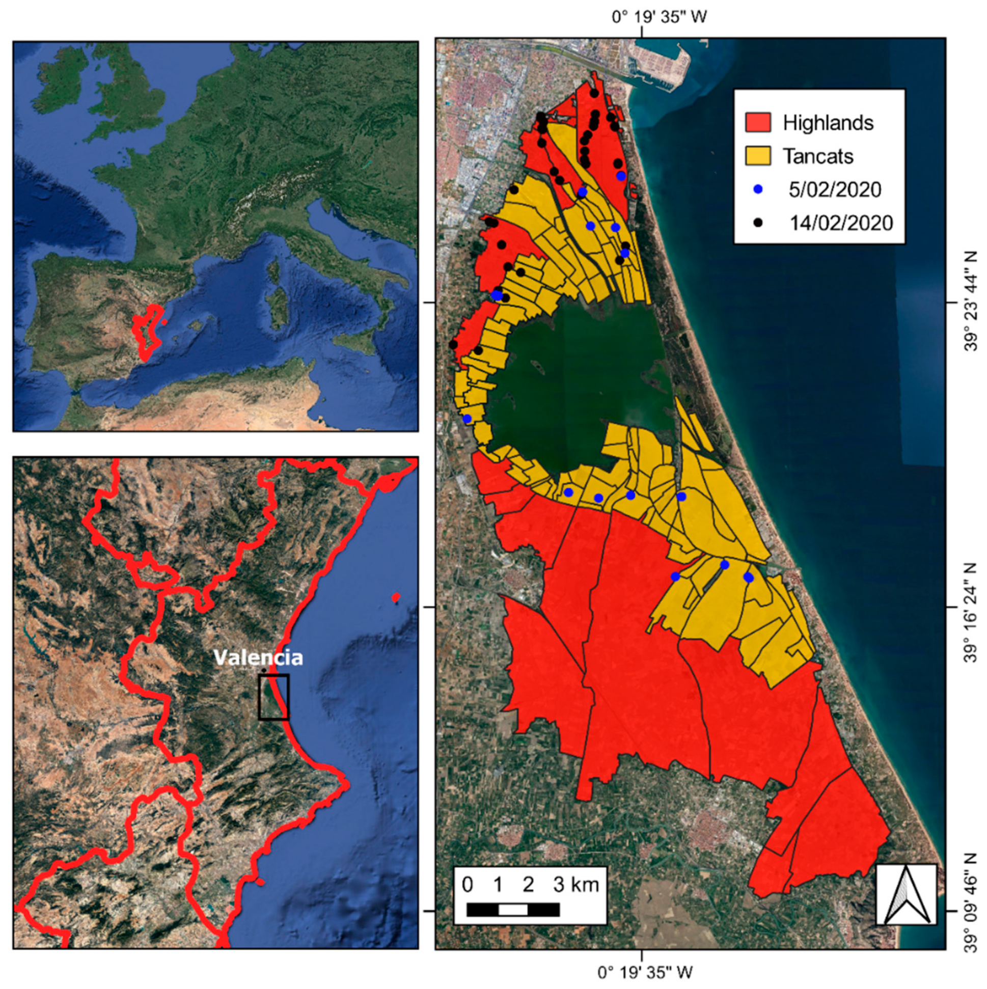
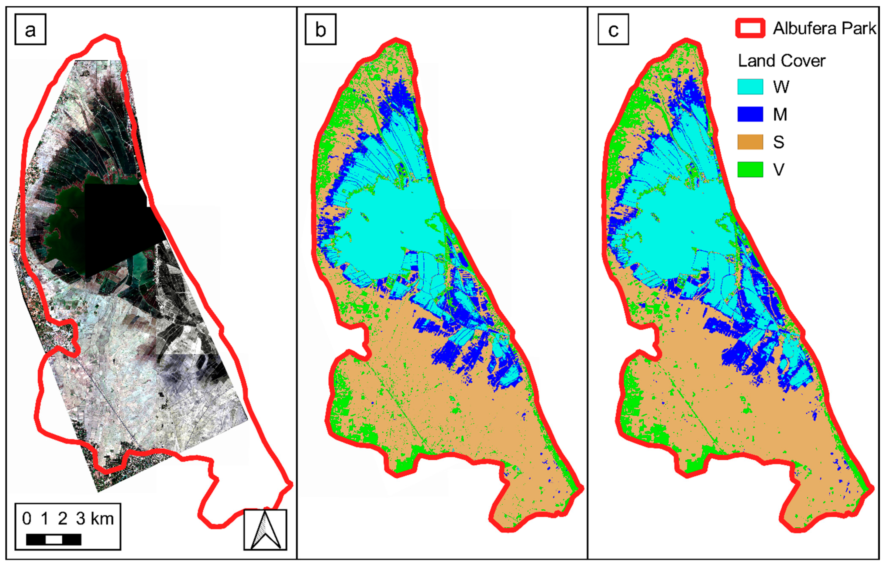
The Albufera is a Mediterranean coastal wetland located 10 km south of the city of Valencia in Spain (Figure 1). This wetland covers an area of 210 km²; it includes the Albufera lake, with a surface of approximately 24 km², and rice fields with an area of around 150 km².

The Albufera wetland was declared Natural Park in 1986 and was included in the Ramsar Convention on “Wetlands of International Importance” in 1989. It is also part of the Natura 2000 network as a Special Protection Area for Birds (SPA) under the Birds Directive 2009/147/EC (site code ES0000471), and a Site of Community Importance (SCI) under Habitats Directive 92/43/EEC (site code ES0000023). The SCI site hosts, in total, 115 species, referred to in Article 4 of the Birds Directive and listed in Annex II of the Habitats Directive. Among them, 64 winter and 35 reproduce in the wetland. Among protected fish species, there are the Spanish Cyprinodont, classified as endangered, and the Valencia Toothcarp, classified as critically endangered. The endangered plants Marsilea and Marsilea Quadrifolia are also present.

From a geological point of view, the site is located in a sedimentary basin of Holocene origin that includes the coastal plain of the province of Valencia. The climate is Mediterranean, with mild winters and warm to hot summers. The average annual precipitation is less than 460 mm, with a maximum in October and a minimum in July.

The Albufera lake is the largest freshwater body on the Iberian Peninsula; it is fed by irrigation channels, storm water streams and urban and industrial wastewater treatment plants. The Albufera lake is connected to the Mediterranean Sea through two natural channels and one artificial channel called “golas”, where sluice gates control the freshwater outflow towards the sea and regulate the water level of the lake. The wetland flooding is managed in two different ways (see Figure 1). The rice fields close to the lake correspond to the traditional area previously occupied by the lake. Earth dikes and pumping stations were introduced to regulate the water level in these lowlands, which are locally called “Tancats”. The highlands, further away from the lake and at higher elevation, are flooded from the Turia and Xuquer Rivers. In addition to these water sources, since 1990, the northern part of the wetland has been irrigated with the outlet of the wastewater treatment plant of Pinedo, located at the northern boundary of the natural park.

Water levels and the extension of the flooding area are regulated by different irrigation communities according to the needs of rice cultivation. There are two flooding periods, in winter and in summer. The summer flooding usually starts in May and ends in mid-September, when the farmers dry up the fields for harvesting. The duration of summer flooding is determined by the rice cultivation technique. Winter flooding starts around the end of October and lasts until the beginning of March. The purposes of winter flooding are to provide habitats for water-related animals and to support recreational activities such as hunting [40]. The winter flooding is economically supported by the European Agricultural Fund for Rural Development (EAFRD). In winter periods, the Tancats are completely flooded with the water level at the top of the dikes and the rice fields are hydraulically connected to each other. Parts of the highlands are also flooded but the water depth may be of the order of a few centimeters only. Given the unpredictability of the duration of winter flooding and its importance for maintaining biodiversity, in this work, we focused specifically on the monitoring of the winter period.

3. Material

We used a set of cloudless Landsat-8 (L8) and Sentinel-2 (S2) images to map land cover classes. In addition, we employed very high-resolution images (VHR) of the GeoEye-1 and WorldView-4 satellites and field data to validate the results obtained from the L8 and S2 images.

3.1. Landsat-8 Dataset

The Landsat mission provides an archive of Earth’s observations by multiple satellites launched in orbit at different times since 1972. Landsat data are provided for free by the joint efforts of the USGS and NASA. The data, acquired from 2013 to 2020 by the Operation Land Imager (OLI) sensor of the L8 satellite, were downloaded from the USGS web portal (https://earthexplorer.usgs.gov/, accessed on 30 August 2021). The OLI sensor acquires 9 spectral bands (see

Table 1. Spectral coverage of the employed satellite data.

Bands [µm]	Sentinel-2	Landsat-8	GeoEye-1	WorldView-4
VIS	0.46−0.52	0.45−0.51 0.53−0.59	0.45–0.51	0.45−0.51
	0.54−0.58	0.64−0.67	0.52–0.58	0.51−0.58
	0.65−0.68		0.65–0.69	0.65−0.69
RED-EDGE	0.698−0.712
	0.733−0.747
	0.773−0.793
NIR	0.784−0.9	0.85−0.88	0.78–0.92	0.78−0.92
	0.855−0.875
SWIR	1.565−1.655	1.57−1.67
	2.1−2.28	2.11−2.29
TIR		10.6−11.2
		11.5−12.5
PAN		0.500−0.680	0.450−0.90	0.450−0.800

), in the visual (VIS, 1-2-3-4 bands), near-infrared (NIR, 5 band) and short-wave infrared (SWIR, 6-7-9 bands). The temporal resolution is around 9 days and the spatial resolution is 30 m, except for the panchromatic band, which has a spatial resolution of 15 m [41]. The surface reflectance of L8 products (Level-2 data products) is generated by the Earth Resources Observation and Science (EROS) center. The on-demand interface EROS Science Processing Architecture (ESPA) corrects satellite images for atmospheric effects through the Land Surface Reflectance Code [42]. In this work, 81 cloud-free images, acquired from 2013 to 2020, from September to April, were used.

3.2. Sentinel-2 Dataset

The Copernicus S2 mission has provided multispectral images of the Earth’s surface since 2015. The free and open access to Sentinel missions’ data is guaranteed by the European Commission (EC) and the ESA. The data products were downloaded from the Copernicus Open Access Hub (https://scihub.copernicus.eu/dhus/#/, last accessed on 30 August 2021). The S2 mission comprises a constellation of two polar-orbiting satellites placed in the same orbit. The first satellite, Sentinel-2A, launched in 2015; it provides images with a revisit time of approximately 10 days. Since the launch of the second satellite, Sentinel-2B, in 2017, the overall revisit time has become around 5 days. Both satellites are equipped with an opto-electronic Multi Spectral Instrument (MSI) that acquires thirteen spectral bands (see Table 1) in the VIS (1-2-3-4 bands), RED-EDGE (5-6-7), NIR (8-8a bands) and SWIR (9-10-11-12 bands). The spatial resolution is 10 m for the 2, 3, 4 and 8 bands; 60 m for the 1, 9 and 10 bands and 20 m for the other bands. S2 collection delivers Top-of-Atmosphere (TOA) reflectance (level-1C) products for data acquired before 2017 and Bottom-of-Atmosphere (BOA) reflectance images (level-2A) for data acquired after 2017 [41]. Therefore, it is necessary to correct the atmospheric effects on the S2 Level 1C images acquired before 2017. The Sen2Cor tool, developed by ESA and Telespazio VEGA Deutschland GmbH, was used for this purpose. In addition, we adopted a bilinear interpolation algorithm, implemented in the Sentinel Application Platform (SNAP) tool, to resample at 10 m all the spectral bands that were originally acquired with lower resolutions. In this work, 69 cloud-free images, acquired from 2015 to 2020, from September to April, were used.

3.3. Very High-Resolution Images

Thanks to their very high spatial resolution, WorldView-4 (WV-4) and GeoEye-1 (GE-1) satellite images can be used as a reference condition to validate the classification tool. These images were provided by the European Space Agency (ESA) in the framework of the ESA third-party mission (© TPMO 2019). The WV-4 and GE-1 satellites were launched in 2016 and 2008, respectively. The WV-4 acquires five spectral bands covering the blue, green, red (VIS) and NIR bands at a resolution of 1.24 m and panchromatic images at a resolution of 0.31 m. GE-1 acquires VIS and NIR bands at 2 m and panchromatic images at 0.5 m. For both WV-4 and GE-1, pan-sharpened images, with a spatial resolution of 50 cm, were used. Details of all bands provided by all the considered missions are given in Table 1.

3.4. Field Data

Field data were also used as ground truths to validate the land cover classification. Geo-located pictures of the area of interest were acquired in various conditions: dry, flooded, with and without vegetation. On 5 February 2020, the photos were taken in correspondence to 18 points located in different parts of the Albufera wetland (see Figure 1). In this survey, the acquisition points were preferentially fixed in correspondence to the Tancats, where, at the time of acquisition, the area was mostly covered by water. On 14 February 2020, 38 geo-located pictures were taken in the north-west of the Albufera at the boundary between the Tancats and the highlands. This area is characterized by a variety of land cover patches. The survey was purposely scheduled on the same day of the WV-4 acquisition and within a few days of the L8 and S2 acquisitions. A set of the acquired pictures, showing the most common land cover types in the winter period, is provided in Section 4.1.

4. Methods

In this work, we jointly used the information acquired by L8 and S2 data in order to reduce the revisit time and consequently improve the temporal continuity of monitoring. The multidisciplinary nature of the project required simple, automatic and robust processing, easily employable also for non-expert users. Given the above-defined goal and constraints, we used a method based on the integration of information retrieved separately from L8 and S2 processing. This choice avoided the implementation of cross-calibration algorithms that could be challenging in the technical applications. The results and the compatibility of the information retrieved by the heterogeneous data were verified by checking the coherence of the land classification obtained by the two datasets (details are reported in Section 4.3).

4.1. Rule-Based Classification of Land Cover Classes

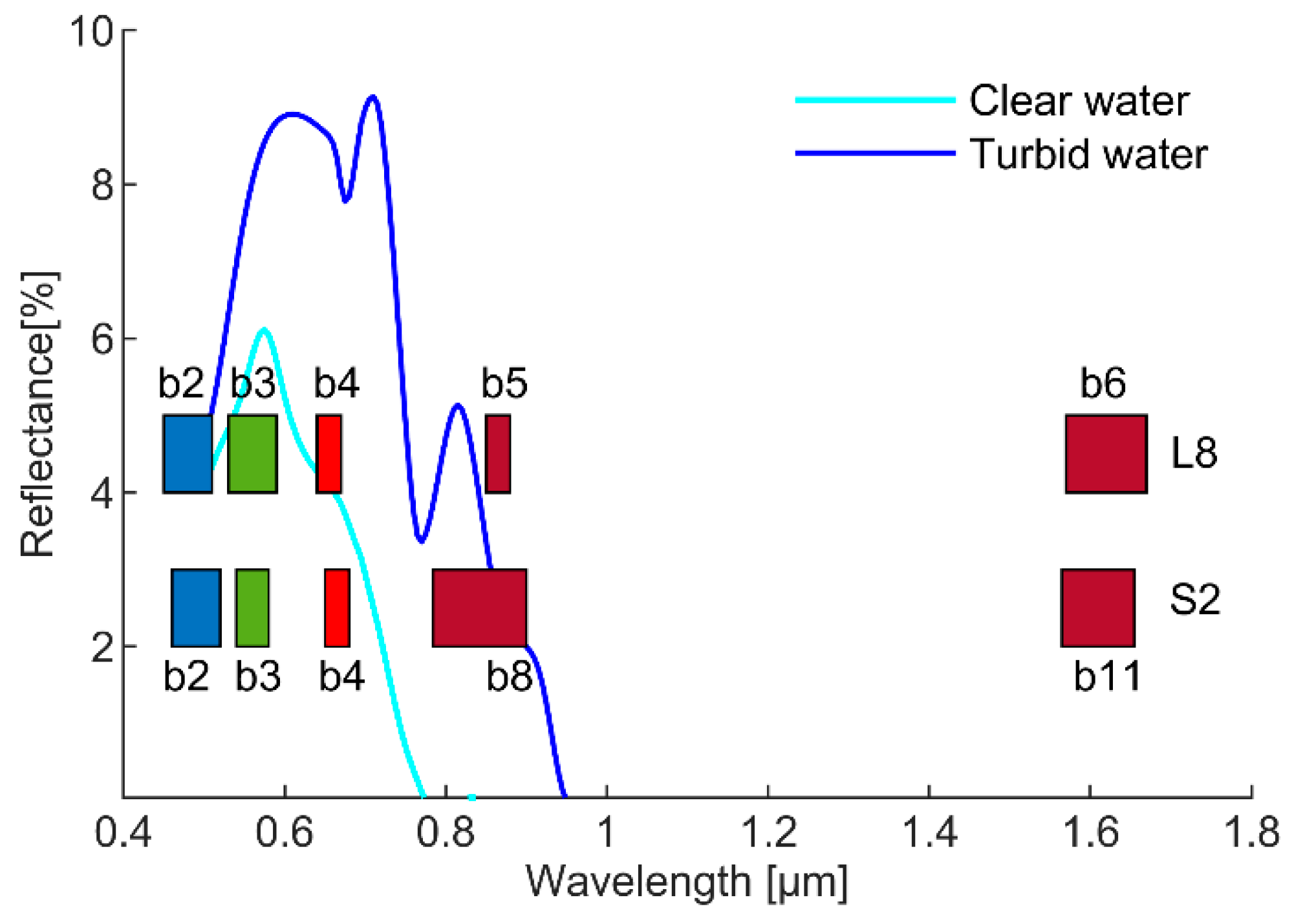
Different types of surfaces, such as water, vegetation, bare soil and urbanized areas, have different reflectivity spectra [43]. The spectrum of water depends on its chemical and physical characteristics. Indeed, the clear water reflectance spectrum peaks in the green wavelength band (0.50–0.56 µm) and decreases against increasing wavelengths, reaching a reflectance close to zero in the near-infrared (NIR) region (0.75–1.4 µm). The turbid water reflectance spectrum exhibits higher values than clear water in the near-infrared region and approaches zero at longer wavelengths [44]. This is due to the concentration of solutes, sediments and organic matter, whose presence reinforces the reflection in the near-infrared band. The above-described patterns are displayed in Figure 2. Typically, the water of wetlands, lakes and rivers contains solid particles and appears not clear. In the case of shallow water, the turbidity of the surface layer can be particularly high. Furthermore, in the case of shallow transparent water, the spectral signature can be influenced by the reflectance of the bed.

The differences in spectral signatures are typically exploited for the automatic classification of land cover, defining appropriate multispectral indices. For instance, the widely used Normalized Difference Water Index (NDWI) [45] is defined as:

$$\mathrm{NDWI}=\frac{{\rho }_{green}-{\rho }_{NIR}}{{\rho }_{green}+{\rho }_{NIR}}$$

(1)

where ρ_green and ρ_NIR are the reflectivity in the green and NIR bands. It can be argued from the spectra presented in Figure 2 that areas covered with clean water will be characterized by positive values of NDWI. On the contrary, it is expected that the surfaces covered by turbid waters will manifest almost null values of NDWI. In contrast, both clean and turbid water will be characterized by positive values of MNDWI [46], which uses the short-wavelength infrared ρ_{SWIR_1} (SWIR) (1.4–3 µm) in place of the NIR reflectivity:

$$\mathrm{MNDWI}=\frac{{\rho }_{green}-{\rho }_{SWIR\_1}}{{\rho }_{green}+{\rho }_{SWIR\_1}}$$

(2)

Along with water indices, the Normalized Difference Vegetation Index (NDVI) [47] is used to identify vegetated areas. The NDVI is defined as a combination of the NIR and visible red (${\rho }_{red}$) to bring out the significant difference in the vegetation spectrum in these bands:

$$\mathrm{NDVI}=\frac{{\rho }_{NIR}-{\rho }_{red}}{{\rho }_{NIR}+{\rho }_{red}}$$

(3)

Following previous literature studies [48,49], we used a threshold of 0.3 to discriminate the presence of vegetation in the observed area. In

Table 2. Specification of bands used in the multispectral indices’ calculation for both data sources.

Landsat-8	Sentinel-2
$\mathrm{NDWI}=\frac{{\rho }_3-{\rho }_5}{{\rho }_3+{\rho }_5}$	$\mathrm{NDWI}=\frac{{\rho }_3-{\rho }_8}{{\rho }_3+{\rho }_8}$
$\mathrm{MNDWI}=\frac{{\rho }_3-{\rho }_6}{{\rho }_3+{\rho }_6}$	$\mathrm{MNDWI}=\frac{{\rho }_3-{\rho }_{11}}{{\rho }_3+{\rho }_{11}}$
$\mathrm{NDVI}=\frac{{\rho }_5-{\rho }_4}{{\rho }_5+{\rho }_4}$	$\mathrm{NDVI}=\frac{{\rho }_8-{\rho }_4}{{\rho }_8+{\rho }_4}$

, the bands used to compute the NDWI, MNDWI and NDVI indices are specified for both the L8 and S2 datasets.

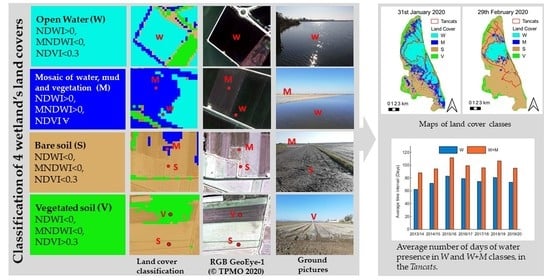
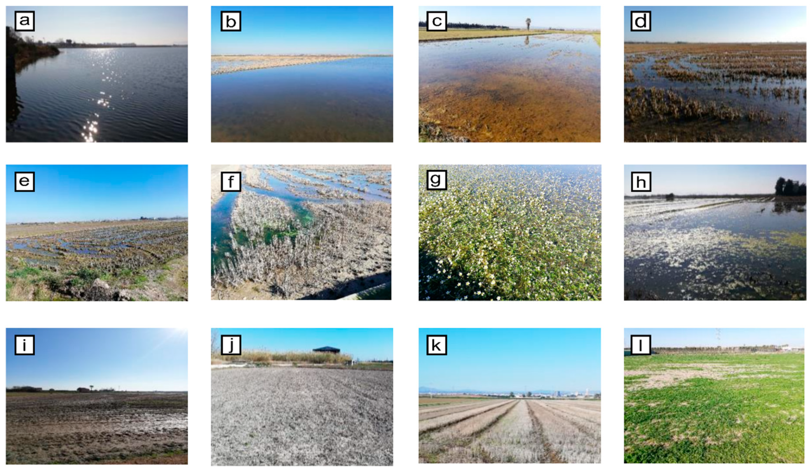
As illustrated in Figure 3, the Albufera wetland’s land cover, in the winter period, is extremely variegated. Considering the classification capacity of the multispectral indices, land cover types were grouped into four classes (see

Table 3. Rule-based classification method for the mapping of the four land cover classes.

Land Cover Classes	Photos	Class	NDWI	MNDWI	NDVI
Open water	a/b	W	>0	>0	<0.3
Mosaic of water, mud and vegetation	c/d/e/f/g/h	M	<0	>0	∀
Bare soil	i/j	S	<0	<0	<0.3
Vegetated soil	k/l	V	<0	<0	>0.3

). In the following, we describe these four classes and the rule-based classification method used to discriminate them.

The first class, labeled “Open water” (W), represents the typical winter condition in the Tancats that are flooded, with water depths ranging from around 0.5 to 1 m (see Figure 3a,b). Note that in some Tancats, dried rice plants could emerge from the shallow water, as shown in the background of Figure 3b. The W class refers to flooded areas with a smooth clear surface and significant depth (higher than approximately 20 cm). In these areas, the sediment content of the water layer close to the surface is low, as shown in the pictures in Figure 3. As the multispectral response is determined by this surface layer, the NDWI results in a positive value. Consequently, the W class can be identified in the satellite images because we expect that the corresponding pixels will exhibit positive values of the water indices (NDWI and MNDWI) and below-threshold values of the vegetation index (NDVI).

In the marginal areas of the wetland, patches of shallow water, mud and vegetation may coexist for transitional periods. As an example, Figure 3e,f show ponds of shallow water surrounded by mud, grass and dead vegetation. Figure 3c shows an area flooded with shallow and turbid water; Figure 3d shows an area flooded with a thin layer of water, from which dry rice plants emerge; Figure 3g,h show flooded areas partially covered with vegetation. All these situations are grouped into the second class, labeled “Mosaic of water, mud and vegetation” (M). These areas can be identified in the satellite images because we expect that the corresponding pixels will exhibit low values of the NDWI, high values of the MNDWI and any value (the ∀ sign) assumed by the NDVI. The third class, labeled “Bare soil” (S), represents wet and dry bare soils (see Figure 3i,j). These areas can be identified in the satellite images because we expect that the corresponding pixels will exhibit low values of the water and vegetation indices.

The fourth class, labeled “Vegetated soil” (V), represents soils partially or entirely covered by vegetation, in wet and dry conditions, as presented in Figure 3k,l. These areas can be identified in the satellite images because we expect that the corresponding pixels will exhibit negative values of the water indices and above-threshold values of the vegetation index.

Based on these considerations, we developed a rule-based classification that allows to distinguish the four classes by exploiting the combination of the responses of the three multispectral indices. The adopted rule-based classification method is summarized in Table 3. The few pixels that do not meet the adopted conditions were considered outliers and labeled as non-classified.

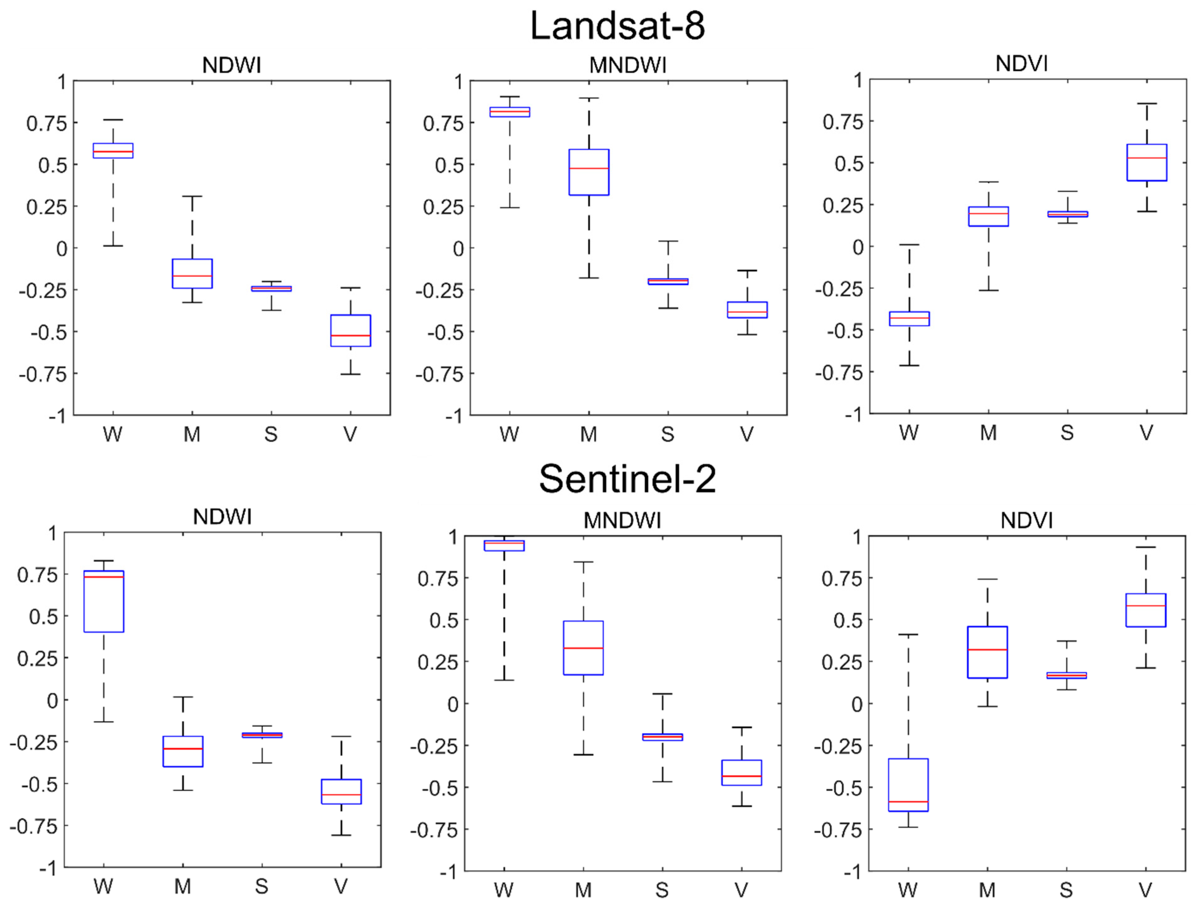
The actual possibility of identifying and distinguishing the four land cover classes was verified by calculating the values of the three multispectral indices for surfaces with known characteristics. These surfaces were mapped by the combined use of VHR images taken on the 14 of February 2020 and geo-located pictures. The detailed procedure for the generation of this ground truth is described in Section 4.2. The results displayed in Figure 4 show that for S2 data, pixels with positive NDWI values can be exclusively associated with the W class. For L8 data, pixels with positive NDWI values can be mostly associated with the W class, with a limited superposition with the M class. Pixels with positive MNDWI values can be only associated with the W and M classes. Pixels with negative MNDWI values can be associated with the V and S classes. Despite small regions of superposition, the MNDWI seems to be able to discriminate the four classes. Pixels with values of NDVI greater than 0.3 represent areas with a significant presence of vegetation and can be mostly associated with the V class. In the case of NDVI, the separability of classes is limited. In particular, the S and M classes are hardly separable with the exclusive use of the NDVI.

In synthesis, we can deduce that, although there is limited overlapping of the values of the indices if applied individually, the joint use of the three indices allows to separate the four classes fairly well.

4.2. Validation Approach

In order to validate the results of the land cover classification method, we compared the classification obtained from S2 and L8 images with the evidence extracted from the VHR images and the field data. Given the slow dynamic of the flooding, the scene can be assumed unchanged in a time interval of few days. Accordingly, we decided to accept the comparison between acquisitions with a maximum of three days of time-lapse. Such an approach led us to define 6 test cases. The acquisition dates of S2, L8, VHR images and field campaigns, of the 6 tests, are shown in

Table 4. Acquisition dates of the data used for the validation tests.

Case No.	Sentinel-2	Landsat-8	Very High-Resolution Image	Field Survey	Spatial Coverage VHR Images
1	15/02/20	13/02/20	14/02/20 GeoEye-1	14/02/20	160 km2—see Figure 5a
2		06/02/20	-	05/02/20	-
3	01/01/19	02/01/19	02/01/19 GeoEye-1	-	43 km2
4	28/10/18	-	25/10/18 WorldView-4	-	28 km2
5	12/03/18	-	13/03/18 WorldView-4	-	22 km2
6	21/01/18	22/01/18	20/01/18 GeoEye-1	-	37 km2

.

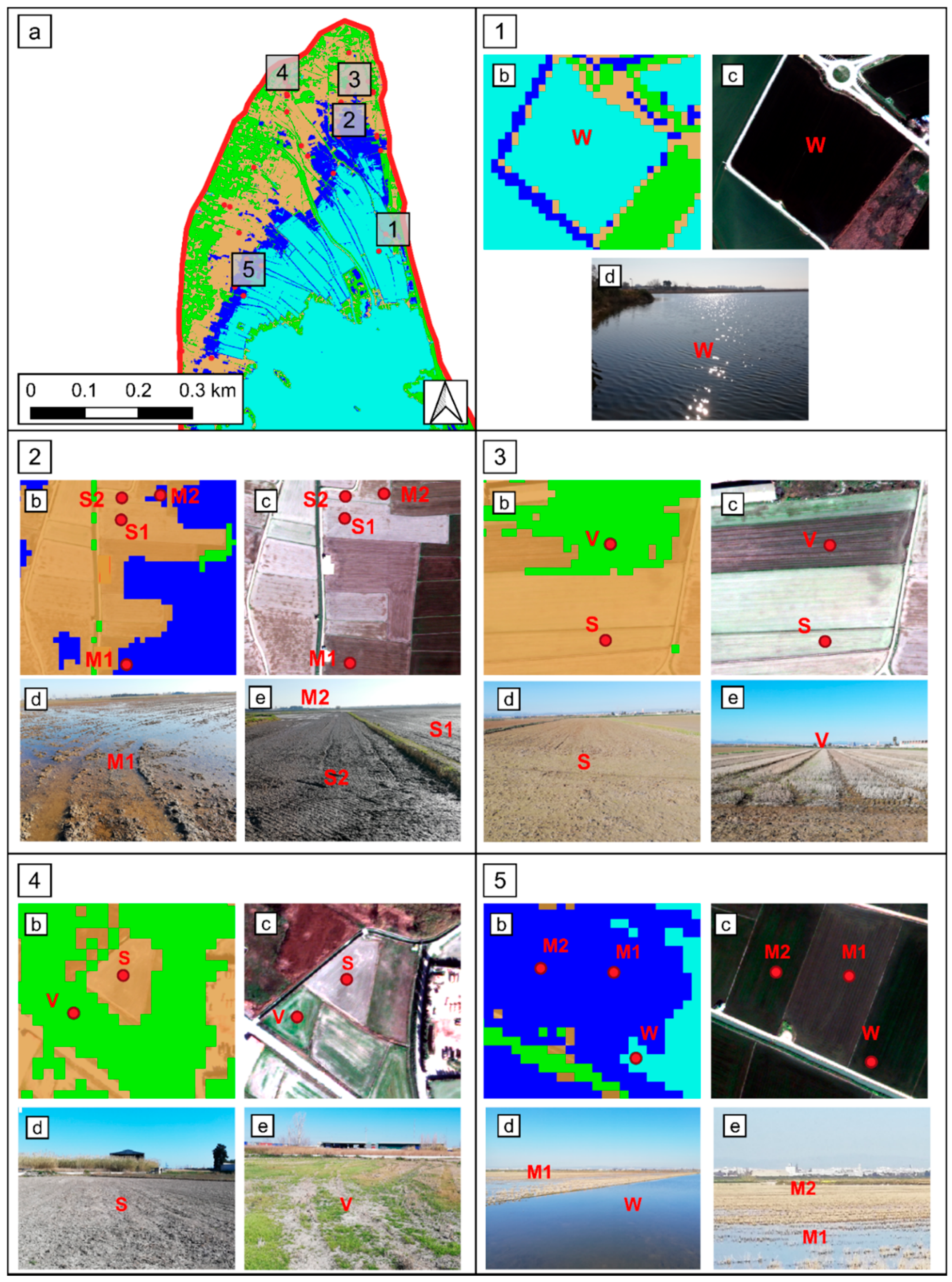
Given the different types and consistencies of the data available on the various cases listed in Table 4, it was necessary to use three different validation approaches. In particular, (i) a pixel-based comparison was employable for case 1, where both VHR images and field pictures were available, (ii) an object-based comparison was possible for case 2 by using only field data as ground truth, and (iii) a more qualitative visual comparison was possible for the cases in which only VHR images were available (cases 3, 4, 5 and 6). The three validation approaches are described below.

In the pixel-based approach, we reported the point of geo-located pictures on the VHR images, and then we manually drew polygons, on the VHR images, to identify the extent of given classes. This operation is based on the visual analysis of the VHR image and therefore depends on the interpretation by the operator. However, the geo-located pictures allow us to identify the type of land use with good accuracy and, once the type is defined, it is quite clear to identify the extension of the assigned type on the VHR image. The manually generated ground truth, thus obtained, was compared on a pixel basis with the predicted land cover classification. The performances were estimated by the computation of the confusion matrix for a multi-class classification [50]. The number of true positive (TPi), false positive (FPi), true negative (TPi) and false negative (FNi) results for the i-th class (W, S, V or M) were computed as follows:

$$T{P}_i=C_{ii}$$

(4)

$$F{P}_i={\displaystyle \sum }_{l=1}^n{C}_{li}-T{P}_i$$

(5)

$$F{N}_i={\displaystyle \sum }_{k=1}^n{C}_{ik}-T{P}_i$$

(6)

$$F{N}_i={\displaystyle \sum }_{l=1}^n{\displaystyle \sum }_{k=1}^n{C}_{lk}-T{P}_i-F{P}_i-F{N}_i$$

(7)

where C_lk is the generic confusion matrix element, the index l relates to the ground truth and the index k refers to the predicted classification. Overall Accuracy, Precision (P_i), Recall (R_i) and F1 score (F1_i) were than computed by:

$$\mathrm{Overall} \mathrm{Accuracy} =\frac{{{\displaystyle \sum }}_{i=1}^n{C}_{ii}}{{{\displaystyle \sum }}_{l=1}^n{{\displaystyle \sum }}_{k=1}^n{C}_{lk}}$$

(8)

$$P_i=\frac{T{P}_i}{T{P}_i+F{P}_i}$$

(9)

$$R_i=\frac{T{P}_i}{T{P}_i+F{N}_i}$$

(10)

$$F{1}_i=2\ast \frac{P_i\ast R_i}{P_i+R_i}$$

(11)

This approach could only be used in case 1, when we have contemporary acquisitions of VHR and ground pictures. The rule-based classification method was applied separately to the L8 image of 13 February 2020 and the S2 image of 15 February 2020, and the results were compared to the ground truth generated by the combination of ground pictures and VHR image.

The object-based approach consisted in the comparison between the predicted classification in a specific area and the land cover shown in the ground pictures for the same area. This approach was used for case 2. The acquisition points are concentrated inside the Tancats (see Figure 1), where water is almost always present in this period (W and M classes), and not enough points are available for the other two classes (S and V). For this reason, the comparison with the ground truth was made only for W and M classes. A two-class confusion matrix was computed and the classification metrics were then estimated by Equations (8)–(11).

The qualitative visual comparison is based on the simultaneous vision of the VHR image and the predicted land cover classification map. This approach is influenced to a greater extent by the interpretation made by the operator and therefore has a lower level of reliability than the other two approaches.

4.3. Consistency Check between the L8 and S2 Datasets

To evaluate the consistency between L8 and S2, the coherence of the land classification obtained by the two datasets was checked. With this aim, S2 and L8 cloud-free images, acquired on the same day, were selected. In the observation period, there are six contemporaneous S2 and L8 acquisitions. For this analysis, we resampled the L8 at the same resolution of the S2 images (10 m) using a bilinear interpolation algorithm. The performances were estimated by comparing each pixel of the so-called predicted condition (L8) with the so-called truth condition (S2). After computation of the confusion matrix, the Overall Accuracy, Precision (P_i), Recall (R_i) and F1 score (F1_i) were estimated with Equations (8)–(11).

4.4. Winter Flooding Duration Maps

The winter flooding duration is key information to evaluate the habitat availability for water-related species. Given the varied management of the wetland, this duration varies from point to point and can be represented with a raster map showing, for each pixel, the number of days in which the corresponding surface was covered with water. For this purpose, we jointly used the L8 and S2 datasets in order to exploit the maximum possible frequency of observation. We first implemented a temporal gap-filling on the MNDWI and NDWI maps. The gap-filling was separately performed on the S2 and L8 datasets to obtain two separate daily series of index values. For each day, the closest S2 or L8 acquisition was identified and the corresponding synthetic map included in the merged series. When the acquisitions S2 and L8 are contemporary, the S2 map is preferred. We used the linear temporal gap-filling proposed by Inglada et al. [51] to monitor vegetative processes and map land coverage through the NDVI on S2 data. This method has the advantage of being easily implemented and more robust than higher-order models. The temporal gap-filling is obtained by:

$$\widehat{I}=\frac{{\Delta }_{+}}{{\Delta }_{-}+{\Delta }_{+}}\cdot I_{-}+\frac{{\Delta }_{-}}{{\Delta }_{-}+{\Delta }_{+}}\cdot I_{+}$$

(12)

where $\widehat{I}$ is the estimated value of the multispectral index (i.e., NDWI and MNDWI) at a specific date, $I_{-}$ and $I_{+}$ are the previous and the subsequent available values, and ${\Delta }_{-}$ and ${\Delta }_{+}$ are the left and right temporal gaps.

Once we had obtained the two daily series of MNDWI and NDWI maps, we applied the rule-based classification to identify the W and M classes. Finally, for each pixel, the number of days per year, in which the W or M class was present, was computed.

5. Results and Validation

5.1. Pixel-Based Quantitative Validation through Comparison with Contemporary Field Data and VHR Images

In this section, we present the results of the quantitative validation, which used both the field and the VHR data (case 1 of Table 4). Figure 5 displays the RGB GeoEye-1 image acquired on 14 February 2020 along with the land cover maps derived by the S2 of 15 February and by the L8 of 13 February. These images show the Albufera wetland in the drying phase, a typical situation at the end of the winter flooding. In this period, several Tancats are still flooded and placed in the W class, while some fields are drying up and are partially or completely in the M class.

Following the procedure described in Section 4.2, 95 polygons of known soil cover classes were drawn for 1136 km², of which 675 km² were in the W class, 165 km² in the M class, 147 km² in the S class and 150 km² in the V class. The ground truth in the W class was found to be larger than the others. This occurred because the identification of the areas in the W class is more straightforward as these areas are clearly visible in the VHR. Furthermore, this class had a greater spatial extension than the others. In

Table 5. Confusion matrix between predicted S2 classification and ground truth.

		Predicted Condition
		W	M	S	V	TOTpixel,i
True condition	W	6691	54	2	0	6747
	M	3	1602	25	17	1647
	S	0	1	1468	2	1471
	V	0	0	72	1429	1501
					TOTpixel	11,366

and

Table 6. Confusion matrix between predicted L8 classification and ground truth.

		Predicted Condition
		W	M	S	V	TOTpixel,i
True condition	W	744	0	1	0	745
	M	25	145	6	1	177
	S	0	2	166	1	169
	V	0	0	9	166	175
					TOTpixel	1266

, the confusion matrices for S2 and L8 classification are reported.

It is worth noting that the pixel number in the ground truth classes was different for L8 and S2 because of the different spatial resolutions of the two datasets. In both the L8 and S2 cases, the confusion matrix was almost diagonal, showing that the rule-based classification method is efficient and reliable. The overall accuracy was very high for both datasets and, in particular, it was 0.985 for S2 and 0.965 for L8. In

Table 7. Performance metrics estimated for S2 land cover classification.

	W	M	S	V
Precision	1.000	0.967	0.937	0.987
Recall	0.992	0.973	0.998	0.952
F1 score	0.996	0.970	0.966	0.969

and

Table 8. Performance metrics estimated for L8 land cover classification.

	W	M	S	V
Precision	0.968	0.986	0.912	0.988
Recall	0.999	0.819	0.982	0.949
F1 score	0.983	0.895	0.946	0.968

, the most relevant performance metrics are presented for S2 and L8, respectively. The precision was always higher than 0.9, with minor differences between the classes: the W class was identified with the highest precision, while the S class was identified with the lowest value. The recall was higher than 0.950 for all the classes except for the M class derived by L8, for which the lowest metric was obtained (0.819). Similar results were obtained for the F1 score, which was always higher than 0.950, except for the M class of L8, for which it was 0.895. The performances obtained with the S2 data were slightly higher than those obtained with the L8 data, as was expected due to the lower spatial resolution of the L8 images. However, the small differences and the high performances for both datasets give a first positive indication in the direction of the joint use of the two datasets. The possibility was also verified by a direct comparison, as reported in Section 5.4.

5.2. Object-Based Quantitative Validation through Comparison with Field Data

In case 2, field data were available, but VHR images were not, and metrics were computed with the object-based procedure, as introduced in Section 4.2. It is worth noting that, in case 2, only the L8 image was available due to the absence of cloud-free S2 acquisition close enough in time. As specified above, in case 2, only a two-class (W and M) confusion matrix was computed. Of the 18 ground objects, one was excluded because it was in the S class, eight were correctly classified as W, eight were correctly classified as M and only one object of the M class was wrongly classified as W. The overall accuracy was 0.941. The F1 score was 0.947 for both the W and M classes. Albeit with a small number of comparisons, the estimated performances confirmed the previous paragraph’s evaluations (case 1).

5.3. Qualitative Validation through Comparison with VHR Images

The qualitative comparison between predicted land cover and VHR images was performed for all the cases in which VHR images were available (see Table 4). The results obtained in the various cases were comparable to each other and all showed satisfactory congruence. For the sake of brevity, we report in this paragraph only two examples, namely case 1 and case 5. Figure 6a reports a detail of the S2 land cover classification in the northern portion of the Albufera Park, for case 1. Figure 6b shows magnified sub-panels of the same map that are compared with the corresponding panels of the VHR image (Figure 6c) and with ground pictures (Figure 6d,e).

In Figure 6(1), an example of an area classified as “Open water” (W) is presented. The peculiar characteristic of the W class is the presence of water depths higher than approximately 20 cm. In this condition, the post-harvest rice plants, if present, are mostly submerged and the surface layer of water is characterized by low turbidity. Therefore, the rice fields are represented as a water body similar to the Albufera lake. As an example, the land cover classification, reported in Figure 6(1b), is in perfect agreement with the VHR (Figure 6(1c)) and the geo-located ground picture (Figure 6(1d)). The classification of Figure 6(2b) shows mosaic of water (M), bare soil (S) and a small vegetated area (V). The M class, frequently encountered at the boundary of the flooded area, is characterized by shallow water depths or a combination of water, mud and vegetation. Regions with ponds smaller than the resolution cell also fall into this class. The S class includes both dry and wet soil as the classification method could not distinguish the two. Looking at the picture of Figure 6(2d), it is possible to note an area (M1) with very shallow water that was correctly classified as the M class. In the picture of Figure 6(2e), bare soil (locations S1 and S2) was present in the foreground. In addition, a small isolated pond (M2) is also visible in the background. All these areas were correctly classified in their relative classes. It is worth noting that the classification could detect the presence of very shallow water (with a depth of few centimeters), pointing out the distinction between M and S, which is very well shown by Figure 6(2b,e).

Figure 6(3,4) display a composite of the S and V classes. Moreover, in these cases, the classification method responded confidently and could detect the vegetation patchiness. Figure 6(5) shows how the method could detect the presence of water mixed with the dry stalks of the cut rice and associated this area with the M class. The adjacent area, in which the water level was higher and there were no stalks emerging from the water surface, was correctly assigned to the W class.

The comparison between the classification obtained from the S2 image of 28 October 2018 and the GE-1 VHR image of 25 October 2018 is presented in Figure 7. W, M, S and V classes appear congruent with what can be deduced from the VHR image.

5.4. Consistency between Classification Maps Derived by L8 and S2

The consistency between the classifications made with L8 and those made with S2 is indirectly verified by the comparisons made in case 1. In fact, in case 1, the classifications obtained from two images, one L8 and one S2, close in time, were separately compared with the ground truth, obtaining satisfactory results for both. Further verification was obtained from direct comparisons between L8 and S2 cloud-free images acquired on the same day. As introduced in the Methods section, the comparison was performed between the land cover maps obtained with the rule-based classification.

Table 9. Performance metrics estimated for “predicted” L8 indices compared with “ground truth” S2 indices.

Date	F1 Score				Overall Accuracy
	W	M	S	V
17 March 2017	0.983	0.869	0.931	0.813	0.912
12 November 2017	0.941	0.572	0.875	0.787	0.853
31 January 2018	0.937	0.847	0.882	0.821	0.884
27 March 2018	0.984	0.552	0.964	0.811	0.944
8 October 2019	0.980	0.350	0.828	0.835	0.848
27 December 2019	0.931	0.796	0.755	0.808	0.848

reports the resulting performance metrics. The overall accuracy ranges from 0.848 to 0.944. The F1 score is always very high (between 0.931 and 0.984) for the W class and is extremely variable for the M class. The value of the F1 score is particularly low in the M class for the acquisitions of October, November and the end of March. In these periods of the year, the presence of water is mainly limited to the Albufera lake and to small, scattered areas. In fact, the portion of pixels classified as the M class by S2 on these dates is only 0.3% on 8 October 2019, 0.4% on 27 March 2018 and 6.5% on 12 November 2017. A high fragmentation of areas with pools or shallow and turbid waters occurs. In this situation, due to the higher resolution of S2 images, it is sometimes possible to distinguish single pixels or small groups of pixels that are in the conditions W, S or V. In contrast, L8 images, characterized by lower spatial resolution, tend to return more frequently the M class, which is intrinsically a mosaic of patches. This impacts the precision and, consequently, the F1 score of the classification for the M class on these dates. The comparison made in the flooding period between December and March gives, for the M class, higher classification performance (F1 score between 0.796 and 0.869). This is also coherent with the high performance obtained in the ground truth check of case 1, performed on 15 February and 13 February. The performances of S and V are less variable in time; the F1 score is between 0.755 and 0.964 for the S class and between 0.787 and 0.835 for the V class. The confusion matrixes showed that L8 places in the V class some pixels labeled by S2 as S class. This is the main source of discrepancy between the results of S2 and L8 for the S and V classes.

The L8 and S2 consistency can also be assessed by comparing the temporal trends of the surfaces, represented in km², for the different classes. In this way, a cross-check with the daily tests described above is also possible and the impact of seasonality can be further assessed. An example is reported in Figure 8, where the temporal trend of land cover types extracted from L8 is compared with the same trends extracted by S2 for 2019/20. On two dates of this period, L8 and S2 were acquired on the same day (8 October 2019 and 27 December 2019). Good agreement between the flooding dynamics (M and W classes) extracted by the two datasets is shown (Figure 8a). In September and October, the W area almost corresponds with the Albufera lake, and the M area is negligible. The L8 and S2 trends are similar even if the F1 score is very low for the M class on the 8 October (see Table 9). The increasing and decreasing trends of the following months are also similar, and this shows that the good performances found for 27 December are stable over time. Figure 8b indicates that the V class mapped by L8 is sometimes more extended than the S2 one (e.g., on 8 October), while the opposite occurs for the S class.

The joint use of the two datasets offered excellent advantages in terms of reducing the revisit time. From September to April of the observation period (2013–2020), the L8 archive contains a total of 166 images, with an average revisit time of around 8 days. Due to the presence of cloud cover, only 81 images with an average revisit time of 18 days were actually employable. The longest time interval between two cloud-free images was 57 days. In the S2 archive, a total of 175 images were available in the period from September to April, with an average revisit time of around 10 days between 2015 and 2017 and 5 days between 2017 and 2020. Due to the presence of the cloud cover, only 69 images with an average revisit time of 16 days were actually employable. The longest time interval between two cloud-free images was 120 days. In the period covered by both missions (2015–2020), the merging of the two datasets led to an effective average revisit time of around 7 days. In addition, the longest time interval between two cloud-free images dropped to 16 days. As an example, the revisit times of the separated and merged datasets in 2019 are shown in Figure 9.

5.5. Observed Land Cover Dynamics

One of the most interesting applications of the rule-based classification method concerns the monitoring of the spatial distribution and the temporal trend of the flooding. This paragraph shows some examples of the information obtained by the merged S2 and L8 dataset from September to April, outside the rice growing period. Figure 10 shows the winter annual flooding trend for the seven years of observation. In addition to the areas in open water conditions (W class), the figure also shows the overall area in which water was present (W + M classes), even if with small thicknesses or in a spatially discontinuous way.

The time evolution of the W area shows similar trends in the different years (Figure 10a). There is an enlargement period in autumn, a maximum extent of around 80 km² (almost the area of the lake plus the area of the Tancats) in December and January and a progressive reduction until March. In September and March, the flooded area is around 24 km², which is the area of the Albufera lake. In some years (2015/16 and 2018/19), the flooding started earlier than other years (at the beginning of October) and had a longer duration. The 2013/14 was the year with the shortest duration of flooding, which had already ended by 12 February.

The overall extension of the W + M area showed a similar trend to the W one, but with more pronounced variations between different years (Figure 10b). The maximum extent of around 120 km² was not reached every year, but the area always exceeded 100 km². The duration and seasonality of the W + M flooding varied from year to year.

As an example, the spatial distribution and temporal dynamics of the land cover of February 2020 are reported in Figure 11. The areas of the four classes W, M, V and S are mapped. Figure 11 well depicts the drying phase. Indeed, the area initially in W conditions progressively empties; for some time, there is still a residual water cover (M class), and it finally dries up completely. The duration of the drying phase varies in space. In the areas further away from the lake, the M conditions are prolonged for longer times.

5.6. Observed Winter Flooding Duration Maps

Figure 12 shows the spatial distribution of the duration of water presence. These figures were obtained with the technique explained in Section 4.4. Figure 12a shows the number of days on which open water (W class) is present. Figure 12b shows the days on which water is present in any condition, even if in shallow layers or discontinuous patches (W class plus M class).

The average duration of open water presence in the Tancats and the highlands, in winter period, is reported in Figure 13. The Tancats are flooded for a period between two and three months depending on the year in question, while the highlands are flooded for shorter periods (around 20 days). The overall presence of water lasts longer; in fact, the period with the presence of the W or M class in the Tancats is in the range of three or even, in some years, almost four months. In the highlands, these conditions last around 40 days, except in 2017/18. This effect can be explained by the particular weather conditions during the winter on the Mediterranean coast. In this area, it is normal to have cold front events with rainfall up to 200 mm in less than 48 h. These storms produce local floods in areas with worse drainage, sometimes correlated with traditional natural springs (named locally “ullals”) with higher water tables. The winter of 2017/2018 was particularly dry, without any cold front event, which can explain the reduction in water in the highlands.

6. Discussion

The classification of wetland land cover from remotely sensed data is particularly complex due to the large spatial and temporal variability of water depth, water turbidity, floating or emerging vegetation and the growth and harvest of crops [23]. Supervised algorithms have been implemented with good results for wetland land cover classification [24,25,52]. In some cases, various land cover classes were identified, as in the present paper. For example, Dronova et al. [35] mapped four land cover classes with an object-based supervised procedure. Nevertheless, the application of supervised methods seems to be limited due to the lack of local training datasets. Very high-resolution images, besides limited availability, do not provide reliable ground truth because the interpretation of the land cover types is uncertain, especially when plants are growing into the water or at the edges of submerged areas. To obtain reliable training samples, it is necessary to support the interpretation of high-resolution images with field surveys. Nevertheless, extensive field data collection is limited because it can be expensive and time-consuming. Unsupervised methods do not have these limitations and are generally characterized by higher transferability and therefore they can be implemented with less effort in different locations.

In this paper, we propose a straightforward and easily applicable, unsupervised, rule-based method for land cover classification in wetlands, exploiting the S2 and L8 datasets. The method is based on the combined use of three multispectral indices (MNDWI, NDWI and NDVI) and can be easily implemented by technicians and water managers with common GIS platforms. Another significant advantage of the proposed method is the possibility of distinguishing four land cover classes that are relevant for the evaluation of habitat availability for water-related animals and plants. The open water (W class) is distinguished from very shallow water or from a mosaic of water pools, vegetation and mud (M class). Adjacent non-water environments are also identified as vegetated land (V class) and bare soil (S class). After spectral analyses, Amani et al. [30] concluded that the spectral indices derived from the NIR, RE and red bands (e.g., NDWI and NDVI) were the most useful spectral bands for the differentiation of wetland land cover. They also found that the SWIR bands helped to discriminate the shallow water class from other wetland classes. In this application, the distribution of index values for the four land cover classes (W, M, S, V) was computed (Figure 4). The analysis showed that the NDWI index is useful to distinguish the open water condition, and the MNDWI allows us to classify the areas characterized by a mosaic of shallow water, mud and vegetation. Finally, the NDVI index allows us to distinguish bare soil from vegetated soil. Therefore, the proposed combination of these indices in a rule-based classification enhances the discrimination properties and reduces the ambiguity of each index. Amani et al. [30] pointed out that the SWIR band is sensitive to the moisture content in soil and vegetation. This could lead to possible misclassification between wet soil and shallow water conditions. However, this aspect was not observed with the index combination proposed in this work (see Figure 4 and Figure 6 and Table 7 and Table 8). Considering the strong spatial and temporal variability of humidity conditions, further analysis, at different times of the year, could help to determine the possible occurrence of misclassification at particular times or locations.

The threshold values that we used for the NDVI, MNDWI and NDWI are literature values and were not calibrated against data of the specific study area. Since these literature values have been verified by different authors in different contexts, it is reasonable to suppose that they are not dependent on the specific study case. Consequently, we believe that the thresholds would still be valid and the classification rules would be applicable in other wetlands with different characteristics. Further analysis could investigate whether and to what extent the accuracy of the results may vary in different contexts. The availability of ground truths is important to relate remotely sensed data to real features and the correct land cover on the ground. The processing of the ground truth data with manual operation or a qualitative comparison by visual inspection can be influenced by the subjective interpretation of the operator. It is worth nothing that, in the present case, the ground truths were used for the validation of the method and not for calibration of the parameters. Consequently, potential subjectivity would affect the performance evaluation and not the classification results. To exploit the different types of data available, we implemented three different procedures for comparing the classification results to ground truth. Of course, different levels of objectivity and reliability correspond to each of the procedures. Undoubtedly, the most stringent validation test for the proposed classification method was the pixel-based one (case 1), in which the ground truth was obtained by the contextual use of geo-located ground pictures and VHR images. The combination of these two different types of data allowed us to obtain a more objective and reliable ground truth than the widespread practice of using only remote images. The overall accuracy was very high for both datasets (0.985 for S2 and 0.965 for L8). The F1 score values were 0.996 (0.983) for the W class, 0.970 (0.895) for the M class, 0.966 (0.946) for the S class and 0.969 (0.968) for the V class. The L8 results are reported in brackets next to the S2 ones. The identification of the M class showed the most significant difference between S2 and L8 metrics (difference between F1 scores higher than 0.02). The slightly lower performance of L8 data in M class identification could be due to the lower spatial resolution of the L8 images, which had the greatest impact when the patchiness of land cover features was higher, as in the M class. Further differences could be due to the slightly different frequency bands acquired by the two sensors. This point was further investigated by comparing L8 and S2 images acquired on the same day, which is discussed below.

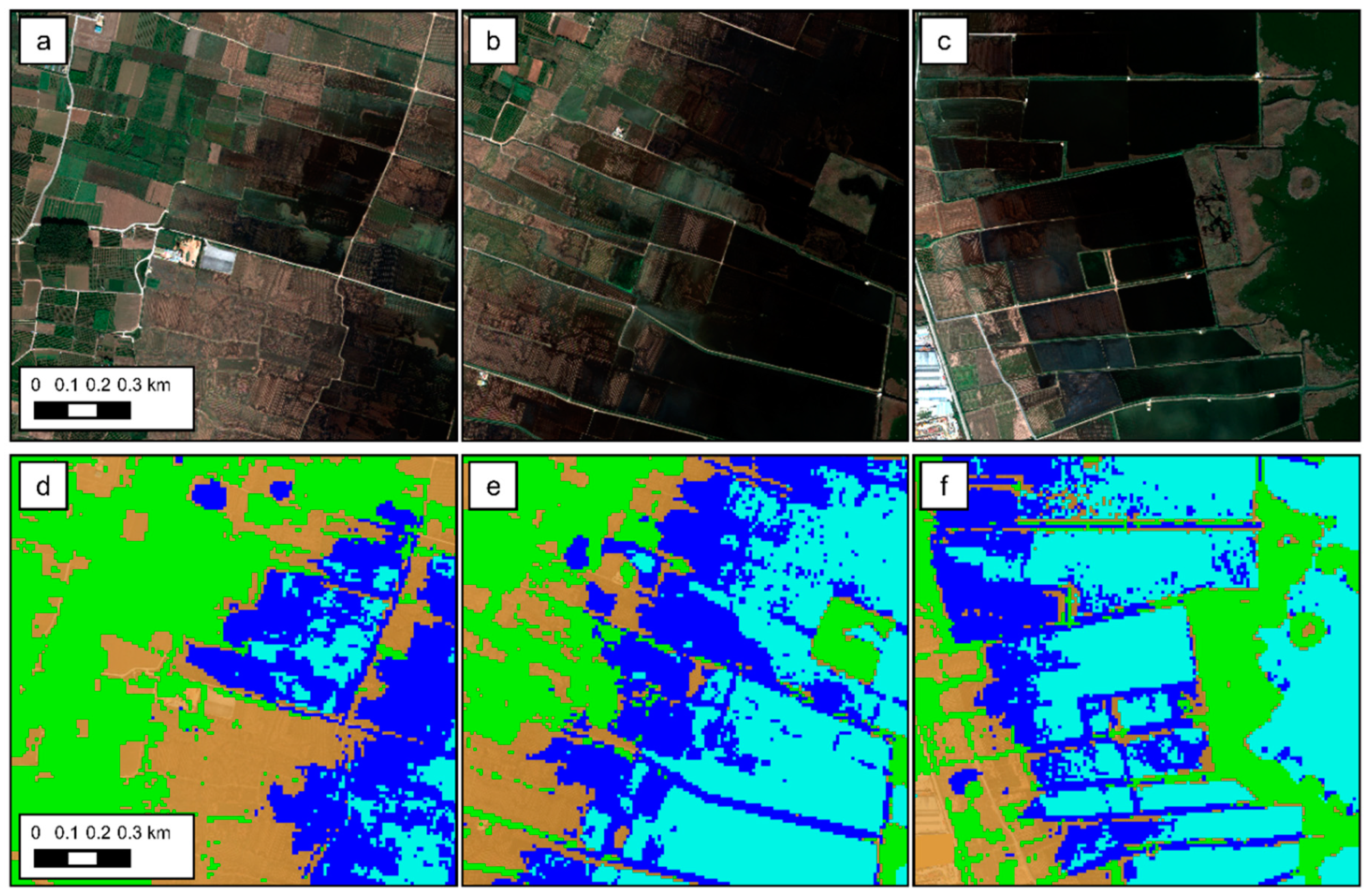
The same ground truth data of case 1 were also used for a visual inspection of the results (see the examples reported in Figure 6). This analysis showed how the method could discriminate surfaces with similar characteristics, such as humid soil and isolated pools of water. Since wetlands are highly variable over time, with a seasonal regime, it was necessary to verify the performance of the classification tool throughout the year. This was done through qualitative validation tests of cases 3, 4, 5 and 6. These validation tests confirmed the high classification capacity of the method and allowed us to verify that the results were stable regardless of the particular conditions of the day of acquisition.

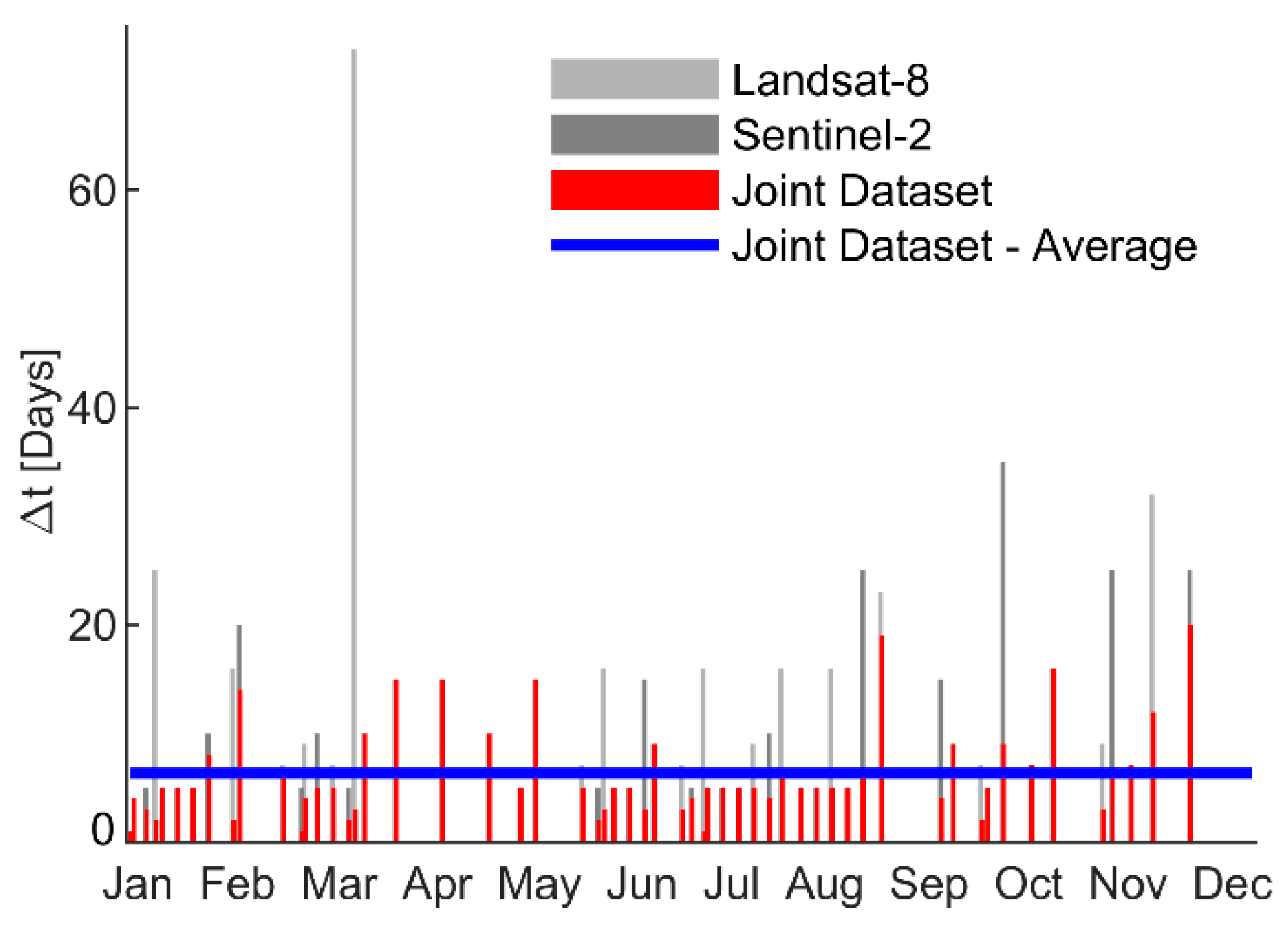
The revisit time of multispectral imagery can be highly impacted by the possible presence of the cloud cover. In order to mitigate this problem, we jointly used the two S2 and L8 datasets. In this way, the average revisit time between two cloud-free images dropped from 18 and 16 days for the L8 and S2 separate datasets to 6 days for the merged dataset. The possibility of integration of the two datasets was investigated by Mandanici and Bitelli [27]. They performed tests on images acquired with a time gap lower than 20 min and demonstrated a good correlation between corresponding bands of the two sensors. However, the radiometric characteristics of the two sensors were not identical. The authors suggested evaluating the impact of such discrepancies for each specific application, depending on the adopted methodology and the aim of the study. In this work, with the objective of providing a tool that is extremely easy to apply, the two datasets were separately processed, and the land cover maps were obtained independently for the S2 and the L8 datasets. To verify the validity of this approach, it is sufficient to verify the coherence between the classification results obtained by the two datasets. The direct comparison of the land cover classification, derived from S2 and L8 acquisitions made on the same days, showed satisfying coherence (overall accuracy between 0.848 and 0.944). The detailed analysis of the performance for the different classes showed that, when the flooding is scarcely present and scattered, pixels classified by L8 as the M class were placed by S2 in other classes. This is probably due to the lower spatial resolution of L8, which induces a sort of spatial average, thus shifting the response towards classes characterized by higher patchiness (i.e., the M class). Another small discrepancy was found between the V and S classes. In particular, L8 tended to classify as V class pixels that S2 classified as S class. These discrepancies may be adjusted by calibrating the threshold of the NDVI index separately for the L8 and S2. 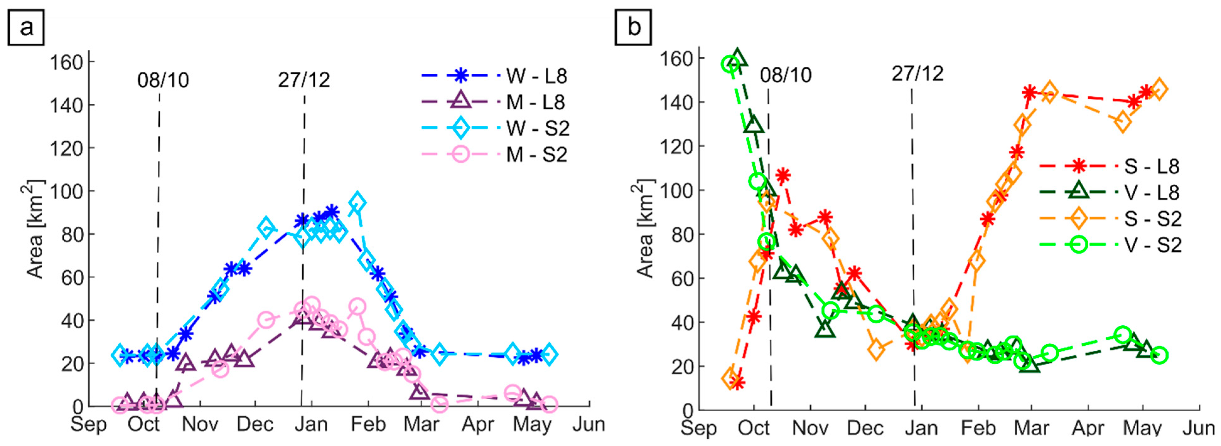A further confirmation of the overall coherence between S2 and L8 classifications is reported in Figure 8, showing that the temporal trends of estimated areas in different classes are similar for the two datasets. This result is particularly significant because it shows how, despite the high dynamism of the wetland context, the coherence between the two datasets was quite stable over time.

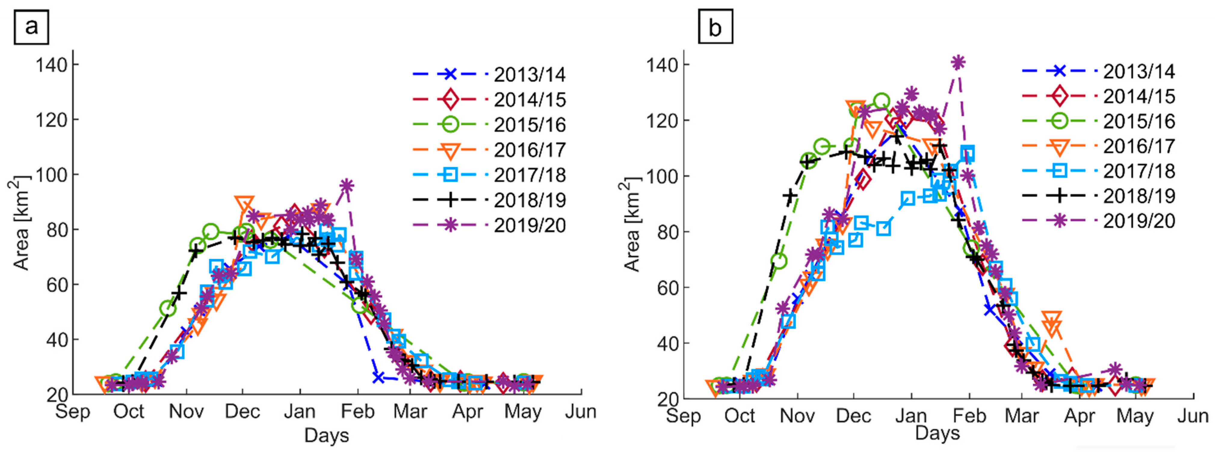
The possibility of mapping the four classes and quantifying the extent of submerged areas (W and M classes) showed interesting aspects of the hydrometric regime of the Albufera wetland. The spatial extension of the W class has an approximately constant trend from year to year, while the surface in the M class is more variable (see Figure 10). This can be explained by the fact that the surface classified as the W class is influenced by agricultural practices. The farmers can dry the rice fields easily and quickly by using pumps and opening the gates that connect the rice fields with the lake. The time at which the rice fields are dried up is decided by the irrigation communities and it is quite constant throughout the years. The variability of the M class over time can be explained by the fact that it may not depend on irrigation and agricultural practices only. Indeed, a mosaic of water, mud and vegetation (M class) can be observed also after intense precipitation or generated by high evapotranspiration.

Land cover maps, such as those shown in Figure 11, can be very useful for observing in detail the spatial distribution of the land cover and its evolution over time. For example, in 2019, the Tancats were flooded with high water depth in January and started emptying from the middle of February. In the southern area, the water depths started decreasing first and lasted until the end of February. Meanwhile, in the northern portion, the decrease began later and was more rapid. This is probably due to the different ways in which the emptying is carried out, as pumps are sometimes used to accelerate the drying up in the Tancats near the lake, while in the areas further away from the lake, the process takes place more slowly. 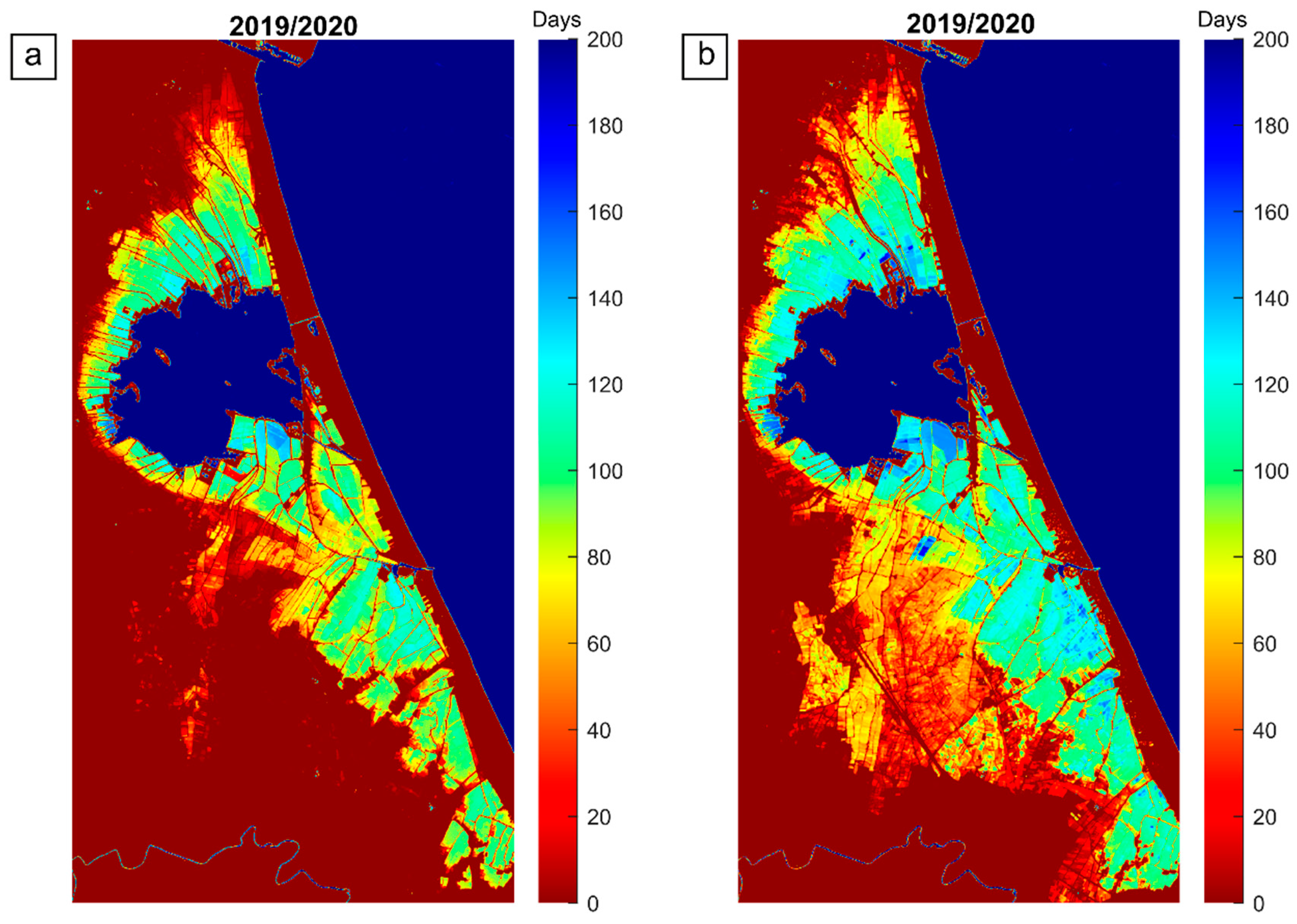Flood duration maps of the kind shown in Figure 12 can be produced for all years of observation and are particularly useful for the estimation of habitat availability for water-related species. The difference between the duration of the W and the M conditions is particularly evident in the highlands. The occasional and sparse presence of the M condition for short time intervals, as shown in Figure 12b, could be due to rainfall events and it can be independent of the artificial management of the wetland.

7. Conclusions

Artificial wetlands play a key role in the strategies to limit the decline of freshwater biodiversity. The timing, duration and extension of periodical flooding are crucial for the survival of many freshwater species. For this reason, continuous monitoring is essential to optimize water resources and quantify habitat availability for water-related organisms. In this work, remote sensing Landsat-8 (L8) and Sentinel-2 (S2) multispectral images were exploited to monitor the Albufera wetland (Spain).

The combination of three multispectral indices, NDWI, MNDWI and NDVI, allowed the implementation of an unsupervised, rule-based method for the automatic classification of four land cover classes: open water (W), mosaic of water, mud and vegetation (M), bare soil (S) and vegetated soil (V). The proposed method is simple and easily usable in practical applications. The MNDWI index, which exploits the SWIR band, allowed to distinguish the M class, characterized by shallow water depths or by patches of water, mud and/or vegetation. The comparison with ground truth data showed overall good agreement (overall accuracy equal to 0.985 for S2 and 0.965 for L8). The validation tests between the L8 and S2 datasets were performed on six days on which both L8 and S2 acquisitions were available. The overall accuracy was always higher than 0.840. The difference in radiometric characteristics and spatial resolution led to small discrepancies in peculiar conditions and classes, such as the occasional overestimation of the M class by the less resolute L8 images.

The joint use of the two datasets provides the advantage of reducing the revisit time; in the analyzed period, the maximum time interval between two cloud-free images was 120 and 57 days for S2 and L8, respectively, while, for the merged dataset, the maximum revisit time was reduced to 16 days.

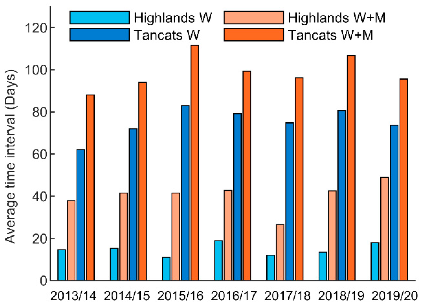
The implemented method allowed to monitor the flooding dynamics of the wetland from 2013 to the present. Both the maximum extent of the flooding and its timing and duration showed differences from year to year. The analyses of the yearly flooding duration showed that the highlands are in the W class, on average, for less than 20 days, and the Tancats are in this class for between 60 and 80 days. Given the short duration of the open water condition (W class), the duration of the time interval in which there are shallow waters or isolated pools (M class) could be crucial for habitat availability. The overall presence of water (M plus W land cover classes) lasted, on average, around 40 days in the highlands and for a period between roughly 90 and 110 days in the Tancats. The automatic land cover classification can be very useful for water management in wetland environments. Monitoring and observing in detail the spatial distribution of submerged areas and their evolution over time may provide important insights that can be used establish the proper timing and duration of flooding in order to support both rice production and habitats for water-related organisms. In wetlands, where there is significant flood risk, the method can also be used to observe the effects of extreme precipitation events and to assess their relative hazard.

References

1. Guo, M.; Li, J.; Sheng, C.; Xu, J.; Wu, L. A Review of Wetland Remote Sensing. Sensors 2017, 17, 777. [Google Scholar] [CrossRef] [PubMed] [Green Version]
2. Matthews, G.V.T. The Ramsar Convention on Wetlands: Its History and Development; Ramsar Convention Bureau: Gland, Switzerland, 1993. [Google Scholar]
3. Gezie, A.; Anteneh, W.; Dejen, E.; Mereta, S.T. Effects of human-induced environmental changes on benthic macroinvertebrate assemblages of wetlands in Lake Tana Watershed, Northwest Ethiopia. Environ. Monit. Assess. 2017, 189, 152. [Google Scholar] [CrossRef]
4. Revenga, C.; Brunner, J.; Henninger, N.; Kassem, K.; Payne, R. Freshwater Systems; World Resources Institute: Washington DC, USA, 2000. [Google Scholar]
5. Perennou, C.; Beltrame, C.; Guelmami, A.; Vives, P.T.; Caessteker, P. Existing areas and past changes of wetland extent in the Mediterranean region: An overview. Ecol. Mediterr. 2012, 38, 53–66. [Google Scholar] [CrossRef]
6. Tourenq, C.; Bennetts, R.E.; Kowalski, H.; Vialet, E.; Lucchesi, J.-L.; Kayser, Y.; Isenmann, P. Are ricefields a good alternative to natural marshes for waterbird communities in the Camargue, southern France? Biol. Conserv. 2001, 100, 335–343. [Google Scholar] [CrossRef]
7. Ma, Z.; Li, B.; Zhao, B.; Jing, K.; Tang, S.; Chen, J. Are artificial wetlands good alternatives to natural wetlands for waterbirds?—A case study on Chongming Island, China. Biodivers. Conserv. 2004, 13, 333–350. [Google Scholar] [CrossRef]
8. Balcombe, C.K.; Anderson, J.T.; Fortney, R.H.; Kordek, W.S. Aquatic macroinvertebrate assemblages in mitigated and natural wetlands. Hydrobiologia 2005, 541, 175–188. [Google Scholar] [CrossRef]
9. Bellio, M.; Kingsford, R.; Kotagama, S. Natural versus artificial-wetlands and their waterbirds in Sri Lanka. Biol. Conserv. 2009, 142, 3076–3085. [Google Scholar] [CrossRef]
10. Pires, M.M.; Kotzian, C.B.; Spies, M.R.; Baptista, V.D.A. Comparative assessment of aquatic macroinvertebrate diversity in irrigated rice fields and wetlands through different spatial scales: An additive partitioning approach. Mar. Freshw. Res. 2016, 67, 368–379. [Google Scholar] [CrossRef]
11. Lawler, S.P. Rice Fields as Temporary Wetlands: A Review. Isr. J. Zool. 2001, 47, 513–528. [Google Scholar] [CrossRef]
12. Pernollet, C.A.; Guelmami, A.; Green, A.J.; Masip, A.C.; Dies, B.; Bogliani, G.; Tesio, F.; Brogi, A.; Gauthier-Clerc, M.; Guillemain, M. A comparison of wintering duck numbers among European rice production areas with contrasting flooding regimes. Biol. Conserv. 2015, 186, 214–224. [Google Scholar] [CrossRef] [Green Version]
13. Stenert, C.; Bacca, R.C.; Maltchik, L.; Rocha, O. Can hydrologic management practices of rice fields contribute to macroinvertebrate conservation in southern Brazil wetlands? Hydrobiologia 2009, 635, 339–350. [Google Scholar] [CrossRef]
14. Baumgartner, D.; Mörtl, M.; Rothhaupt, K.-O. Effects of water-depth and water-level fluctuations on the macroinvertebrate community structure in the littoral zone of Lake Constance. In Ecological Effects of Water-Level Fluctuations in Lakes; Springer: Dordrecht, The Netherlands, 2008; pp. 97–107. [Google Scholar] [CrossRef] [Green Version]
15. White, E.D.; Reed, D.J.; Meselhe, E.A. Modeled Sediment Availability, Deposition, and Decadal Land Change in Coastal Louisiana Marshes under Future Relative Sea Level Rise Scenarios. Wetlands 2019, 39, 1233–1248. [Google Scholar] [CrossRef]
16. Preston, T.M.; Borgreen, M.J.; Ray, A.M. Effects of brine contamination from energy development on wetland macroinvertebrate community structure in the Prairie Pothole Region. Environ. Pollut. 2018, 239, 722–732. [Google Scholar] [CrossRef] [PubMed]
17. Burger, M.; Van Vuren, J.H.J.; De Wet, L.; Nel, A. A comparison of water quality and macroinvertebrate community structure in endorheic depression wetlands and a salt pan in the Gauteng province, South Africa. Environ. Monit. Assess. 2018, 191, 14. [Google Scholar] [CrossRef] [PubMed]
18. Kim, D.-K.; Jo, H.; Park, K.; Kwak, I.-S. Assessing Spatial Distribution of Benthic Macroinvertebrate Communities Associated with Surrounding Land Cover and Water Quality. Appl. Sci. 2019, 9, 5162. [Google Scholar] [CrossRef] [Green Version]
19. Schad, A.N.; Kennedy, J.H.; Dick, G.O.; Dodd, L. Aquatic macroinvertebrate richness and diversity associated with native submerged aquatic vegetation plantings increases in longer-managed and wetland-channeled effluent constructed urban wetlands. Wetl. Ecol. Manag. 2020, 28, 461–477. [Google Scholar] [CrossRef]
20. Machado, I.; Maltchik, L. Can management practices in rice fields contribute to amphibian conservation in southern Brazilian wetlands? Aquat. Conserv. Mar. Freshw. Ecosyst. 2009, 20, 39–46. [Google Scholar] [CrossRef]
21. Elphick, C.S. Functional Equivalency between Rice Fields and Seminatural Wetland Habitats. Conserv. Biol. 2000, 14, 181–191. [Google Scholar] [CrossRef] [Green Version]
22. Tajiri, H.; Ohkawara, K. The Effects of Flooding and Plowing on Foraging Site Selection by Wintering Dabbling Ducks in Rice Fields. Ornithol. Sci. 2013, 12, 127–136. [Google Scholar] [CrossRef]
23. Ozesmi, S.L.; Bauer, M.E. Satellite remote sensing of wetlands. Wetl. Ecol. Manag. 2002, 10, 381–402. [Google Scholar] [CrossRef]
24. Rebelo, L.-M.; Finlayson, C.; Nagabhatla, N. Remote sensing and GIS for wetland inventory, mapping and change analysis. J. Environ. Manag. 2009, 90, 2144–2153. [Google Scholar] [CrossRef]
25. Munyati, C. Wetland change detection on the Kafue Flats, Zambia, by classification of a multitemporal remote sensing image dataset. Int. J. Remote Sens. 2000, 21, 1787–1806. [Google Scholar] [CrossRef]
26. Yang, X.; Liu, Z. Using satellite imagery and GIS for land-use and land-cover change mapping in an estuarine watershed. Int. J. Remote Sens. 2005, 26, 5275–5296. [Google Scholar] [CrossRef]
27. Mandanici, E.; Bitelli, G. Preliminary Comparison of Sentinel-2 and Landsat 8 Imagery for a Combined Use. Remote Sens. 2016, 8, 1014. [Google Scholar] [CrossRef] [Green Version]
28. Carrasco, L.; O’Neil, A.W.; Morton, R.D.; Rowland, C.S. Evaluating Combinations of Temporally Aggregated Sentinel-1, Sentinel-2 and Landsat 8 for Land Cover Mapping with Google Earth Engine. Remote Sens. 2019, 11, 288. [Google Scholar] [CrossRef] [Green Version]
29. Wang, Q.; Blackburn, G.A.; Onojeghuo, A.O.; Dash, J.; Zhou, L.; Zhang, Y.; Atkinson, P. Fusion of Landsat 8 OLI and Sentinel-2 MSI Data. IEEE Trans. Geosci. Remote Sens. 2017, 55, 3885–3899. [Google Scholar] [CrossRef] [Green Version]
30. Amani, M.; Salehi, B.; Mahdavi, S.; Brisco, B. Spectral analysis of wetlands using multi-source optical satellite imagery. ISPRS J. Photogramm. Remote Sens. 2018, 144, 119–136. [Google Scholar] [CrossRef]
31. Davranche, A.; Poulin, B.; Lefebvre, G. Mapping flooding regimes in Camargue wetlands using seasonal multispectral data. Remote Sens. Environ. 2013, 138, 165–171. [Google Scholar] [CrossRef] [Green Version]
32. Li, W.; Du, Z.; Ling, F.; Zhou, D.; Wang, H.; Gui, Y.; Sun, B.; Zhang, X. A Comparison of Land Surface Water Mapping Using the Normalized Difference Water Index from TM, ETM+ and ALI. Remote Sens. 2013, 5, 5530–5549. [Google Scholar] [CrossRef] [Green Version]
33. Li, L.; Vrieling, A.; Skidmore, A.; Wang, T.; Muñoz, A.-R.; Turak, E. Evaluation of MODIS Spectral Indices for Monitoring Hydrological Dynamics of a Small, Seasonally-Flooded Wetland in Southern Spain. Wetlands 2015, 35, 851–864. [Google Scholar] [CrossRef] [Green Version]
34. Forkuor, G.; Hounkpatin, O.K.L.; Welp, G.; Thiel, M. High Resolution Mapping of Soil Properties Using Remote Sensing Variables in South-Western Burkina Faso: A Comparison of Machine Learning and Multiple Linear Regression Models. PLoS ONE 2017, 12, e0170478. [Google Scholar] [CrossRef]
35. Dronova, I.; Gong, P.; Wang, L. Object-based analysis and change detection of major wetland cover types and their classification uncertainty during the low water period at Poyang Lake, China. Remote Sens. Environ. 2011, 115, 3220–3236. [Google Scholar] [CrossRef]
36. Mahdavi, S.; Salehi, B.; Granger, J.; Amani, M.; Brisco, B.; Huang, W. Remote sensing for wetland classification: A comprehensive review. GIScience Remote Sens. 2018, 55, 623–658. [Google Scholar] [CrossRef]
37. Lopez-Garcia, M.J.; Caselles, V. Use of Thematic Mapper data to assess water quality in Albufera Lagoon of Valencia (Spain). In Proceedings of the 13th Annual Conference of the Remote Sensing Society, Nottingham, UK, 7–11 September 1987; pp. 510–519. [Google Scholar]
38. Dona, C.; Chang, N.-B.; Caselles, V.; Sánchez, J.M.; Camacho, A.; Delegido, J.; Vannah, B.W. Integrated satellite data fusion and mining for monitoring lake water quality status of the Albufera de Valencia in Spain. J. Environ. Manag. 2015, 151, 416–426. [Google Scholar] [CrossRef] [Green Version]
39. Sòria-Perpinyà, X.; Vicente, E.; Urrego, P.; Pereira-Sandoval, M.; Ruíz-Verdú, A.; Delegido, J.; Soria, J.; Moreno, J. Remote sensing of cyanobacterial blooms in a hypertrophic lagoon (Albufera of València, Eastern Iberian Peninsula) using multitemporal Sentinel-2 images. Sci. Total Environ. 2020, 698, 134305. [Google Scholar] [CrossRef]
40. Soria, J.; Vera-Herrera, L.; Calvo, S.; Romo, S.; Vicente, E.; Sahuquillo, M.; Sòria-Perpinyà, X. Residence Time Analysis in the Albufera of Valencia, a Mediterranean Coastal Lagoon, Spain. Hydrology 2021, 8, 37. [Google Scholar] [CrossRef]
41. Djamai, N.; Fernandes, R.; Weiss, M.; McNairn, H.; Goïta, K. Validation of the Sentinel Simplified Level 2 Product Prototype Processor (SL2P) for mapping cropland biophysical variables using Sentinel-2/MSI and Landsat-8/OLI data. Remote Sens. Environ. 2019, 225, 416–430. [Google Scholar] [CrossRef]
42. Vermote, E.; Justice, C.; Claverie, M.; Franch, B. Preliminary analysis of the performance of the Landsat 8/OLI land surface reflectance product. Remote Sens. Environ. 2016, 185, 46–56. [Google Scholar] [CrossRef] [PubMed]
43. Ma, S.; Zhou, Y.; Gowda, P.H.; Dong, J.; Zhang, G.; Kakani, V.G.; Wagle, P.; Chen, L.; Flynn, K.C.; Jiang, W. Application of the water-related spectral reflectance indices: A review. Ecol. Indic. 2019, 98, 68–79. [Google Scholar] [CrossRef]
44. Malinowski, R.; Groom, G.; Schwanghart, W.; Heckrath, G. Detection and Delineation of Localized Flooding from WorldView-2 Multispectral Data. Remote Sens. 2015, 7, 14853–14875. [Google Scholar] [CrossRef] [Green Version]
45. McFeeters, S.K. The use of the Normalized Difference Water Index (NDWI) in the delineation of open water features. Int. J. Remote Sens. 1996, 17, 1425–1432. [Google Scholar] [CrossRef]
46. Xu, H. Modification of normalised difference water index (NDWI) to enhance open water features in remotely sensed imagery. Int. J. Remote Sens. 2006, 27, 3025–3033. [Google Scholar] [CrossRef]
47. Curran, P.J. Multispectral remote sensing for the estimation of green leaf area index. In Philosophical Transactions of the Royal Society of London. Series A, Mathematical and Physical Sciences; Royal Society: London, UK, 1983; Volume 309, pp. 257–270. [Google Scholar] [CrossRef]
48. Holben, B.N. Characteristics of maximum-value composite images from temporal AVHRR data. Int. J. Remote Sens. 1986, 7, 1417–1434. [Google Scholar] [CrossRef]
49. Rutkay, A.T.U.N.; Kalkan, K.; Gürsoy, Ö. Determining the forest fire risk with sentinel 2 images. Turk. J. Geosci. 2020, 1, 22–26. [Google Scholar]
50. Story, M.; Congalton, R.G. Accuracy assessment: A user’s perspective. Photogramm. Eng. Remote Sens. 1986, 52, 397–399. [Google Scholar]
51. Inglada, J.; Arias, M.; Tardy, B.; Hagolle, O.; Valero, S.; Morin, D.; Dedieu, G.; Sepulcre, G.; Bontemps, S.; Defourny, P.; et al. Assessment of an Operational System for Crop Type Map Production Using High Temporal and Spatial Resolution Satellite Optical Imagery. Remote Sens. 2015, 7, 12356–12379. [Google Scholar] [CrossRef] [Green Version]
52. Dechka, J.A.; Franklin, S.E.; Watmough, M.D.; Bennett, R.P.; Ingstrup, D.W. Classification of wetland habitat and vegetation communities using multi-temporal Ikonos imagery in southern Saskatchewan. Can. J. Remote Sens. 2002, 28, 679–685. [Google Scholar] [CrossRef]
Figure 1. Overview of the Albufera wetland (© Google 2020) and outline of the rice fields with lower (Tancats) and higher elevation (highlands). The points represent the locations of field surveys performed on 5 February 2020 and 14 February 2020.
Remotesensing 13 03525 g001
Figure 2. Spectral reflectance of clear and turbid water compared to L8 and S2 acquired bands.
Remotesensing 13 03525 g002
Figure 3. Photographs of land cover classes taken in the Albufera wetland on 14 February 2020; (a,b) water; (c) shallow turbid water; (d) shallow water with dead vegetation; (e,f) mosaic of water ponds, mud and vegetation; (g,h) flooded area partially covered by vegetation; (i) wet soil; (j) dry soil; (k,l) vegetated soil.
Remotesensing 13 03525 g003
Figure 4. Distribution of indices values for the four land cover classes (W, M, S, V).
Remotesensing 13 03525 g004
Figure 5. (a) RGB GeoEye-1 of 14 February 2020 provided by ESA (© TPMO 2020); (b) Land cover classification extracted by S2 image of 15 February 2020; (c) Land cover classification extracted by L8 image of 13 February 2020.
Remotesensing 13 03525 g005
Figure 6. (a) Land cover classification extracted by S2 image of 15 February 2020 with field survey locations of 14 February (points) and the position of the frames displayed with larger scales in the panels 1,2 3, 4 and 5; (b) zoom of land cover classification; (c) zoom of the RGB GeoEye-1 (© TPMO 2020) of 14 February; (d,e) ground pictures taken on 14 February.
Remotesensing 13 03525 g006
Figure 7. Comparison between GE-1 VHR of 25 October 2018 (ac) and land cover classification extracted by S2 image of 28 October 2018 (df).
Remotesensing 13 03525 g007
Figure 8. (a) Extent of W, M areas extracted by L8 and S2 in 2019/2020; (b) extent of S and V areas extracted by L8 and S2 in 2019/2020.
Remotesensing 13 03525 g008
Figure 9. Number of days between two usable images of the L8 and S2 datasets taken individually and of the merged dataset in 2019.
Remotesensing 13 03525 g009
Figure 10. (a) Temporal trend of area in W class (open water); (b) temporal trend of area in W or M class (open water or mosaic of water, mud and vegetation).
Remotesensing 13 03525 g010
Figure 11. Maps of land cover classes in February 2020 obtained by L8 and S2. The continuous line is the boundary of Tancats area.
Remotesensing 13 03525 g011
Figure 12. Days of water presence from October to April in 2019/20; (a) W class; (b) W class plus M class.
Remotesensing 13 03525 g012
Figure 13. Average number of days of water presence in W and W + M classes, in the Tancats and in the highlands.
Remotesensing 13 03525 g013