
Boosting Few-Shot Hyperspectral Image Classification Using Pseudo-Label Learning
by
 , , and
Chen Ding
1,2,3 ,
,
Yu Li
4,5,
Yue Wen
4,5,
Mengmeng Zheng
1,2,3,
Lei Zhang
4,5,
Wei Wei
4,5,* and
Yanning Zhang
4,5 1
School of Computer Science and Technology, Xi’an University of Posts and Telecommunications, Xi’an 710121, China
2
Shaanxi Key Laboratory of Network Data Analysis and Intelligent Processing, Xi’an 710121, China
3
Xi’an Key Laboratory of Big Data and Intelligent Computing, Xi’an 710121, China
4
Shaanxi Key Lab of Speech & Image Information Processing (SAIIP), School of Computer Science and Engineering, Northwestern Polytechnical University, Xi’an 710129, China
5
National Engineering Laboratory for Integrated Aero-Space-Ground-Ocean Big Data Application Technology, Xi’an 710129, China
*
Author to whom correspondence should be addressed.
Remote Sens. 2021, 13(17), 3539; https://0-doi-org.brum.beds.ac.uk/10.3390/rs13173539
Submission received: 11 August 2021
/
Revised: 1 September 2021
/
Accepted: 3 September 2021
/
Published: 6 September 2021
Abstract
:Deep neural networks have underpinned much of the recent progress in the field of hyperspectral image (HSI) classification owing to their powerful ability to learn discriminative features. However, training a deep neural network often requires the availability of a large number of labeled samples to mitigate over-fitting, and these labeled samples are not always available in practical applications. To adapt the deep neural network-based HSI classification approach to cases in which only a very limited number of labeled samples (i.e., few or even only one labeled sample) are provided, we propose a novel few-shot deep learning framework for HSI classification. In order to mitigate over-fitting, the framework borrows supervision from an auxiliary set of unlabeled samples with soft pseudo-labels to assist the training of the feature extractor on few labeled samples. By considering each labeled sample as a reference agent, the soft pseudo-label is assigned by computing the distances between the unlabeled sample and all agents. To demonstrate the effectiveness of the proposed method, we evaluate it on three benchmark HSI classification datasets. The results indicate that our method achieves better performance relative to existing competitors in few-shot and one-shot settings.
1. Introduction
Hyperspectral images (HSIs) collect the continuous reflectance of the imaging scene under a wide spectral range, which is often represented as a three-dimensional (3D) data cube and consists of hundreds of narrow spectral bands with a high spectral resolution [1]. Because they contain abundant spectral information, HSIs have been widely employed in many remote sensing-related applications [1,2,3,4,5,6], including environmental monitoring, target localization, military surveillance, and terrain classification, etc.
Among the various HSI-related applications, one of the most essential tasks is HSI classification, which aims at assigning a predefined class label to each pixel. Although many conventional machine learning-based methods, e.g., support vector machine (SVM) and k-nearest neighbors ( NN) [7] etc., have been proposed for HSI classification, the inherently shallow structures of their feature extraction models prevent these methods from learning discriminative features, as well as from appropriately generalizing to challenging cases. As a result, performance may be further improved. Other mathematics based methods are also used in the HSI classification tasks with effective results [8,9].
Unlike conventional machine learning-based methods, deep neural networks can cast feature representation and classifier construction to train an end-to-end hierarchical network with labeled samples. Due to their deep structures, deep neural networks have the powerful ability to learn discriminative features for classification [10,11,12,13,14,15]. To date, extensive deep neural network-based methods for HSI classification [16,17,18,19,20,21] have been proposed and have achieved promising classification performance. For example, Liang et al. [16] propose extracting the deep feature representation of the samples using a stacked denoising auto encoder (SDAE), which is learned without supervision, to then predict the label of samples with a trained back-propagation network under supervision. In [18], Lakhal et al. introduce a deep recurrent neural network that incorporates high-level feature descriptors to tackle the challenging HSI classification problem. After witnessing the success of deep convolution neural networks (DCNNs) in various computer vision tasks [22,23], an increasing number of deep HSI classification methods have adopted the DCNN structure as their backbone. For example, Chen et al. [22] employed several 3D convolutional and pooling layers for deep feature extraction. Moreover, several other strategies to mitigate over-fitting, such as regularization and dropout, have been investigated. In [23], Gong et al. propose integrating the DCNN with multi-scale convolution with determinantal point process-based diversity-promoting deep metrics to obtain discriminative features for HSI classification. Recent progress has shown that due to the gradient vanishing problem, it is difficult to train a deep neural network as the network depth increases. To address this problem, He et al. [24] proposed a novel residual learning structure that can successfully mitigate the gradient vanishing problem. Inspired by this, many recent HSI classification methods have also begun to take advantage of residual learning for training deeper neural networks. For example, Zhang et al. [25] employed a 3D densely connected convolutional neural network (3D-DenseNet) to learn the spectral-spatial features of HSIs for classification. With its densely connected structure, the deeper network can be easier to train. Zhong et al. [26] develop an end-to-end spectral-spatial residual network (SSRN) that takes raw 3D cubes as input data, then employs residual blocks to connect every other 3D convolutional layer through identity mapping for HSI classification purposes.
Compared with conventional machine learning-based HSI classification methods, deep neural network-based methods often achieve much better performance. In order to succeed, these approaches require the network to be trained with sufficient labeled samples. In the HSI classification task, labeled samples are obtained by manually annotating some samples in the given HSI data set with a set of predefined class labels. In practice, since manually annotating an HSI pixel is generally laborious, time-consuming, and can only be accomplished by experts, the labeled samples obtained are always insufficient or even deficient. In such cases, the trained networks are prone to be overfitting (i.e., fail to appropriately generalize to the unseen test samples). To alleviate this problem, some transfer learning-based methods [27,28,29] have been developed. These methods aim to train on an HSI dataset (i.e., source domain) and classify the pixels of same classes on another HSI dataset (i.e., target domain).
However, this kind of method requires a large number of labeled samples to be available in the source domain, which is still unfeasible for lots of applications. Thus, some methods [30,31,32] propose utilizing data augmentation to increase the number of labeled training samples on the given dataset (i.e., target domain), without relying on another, similar dataset (i.e., source domain). For example, in [30], Li et al. proposed to substantially increase the number of labeled training samples using a novel pixel-pair strategy, which combines two pixels (to form a pair of pixels) and then classifies the pixel-pair using a trained DCNN. Although methods of this kind can generate more labeled samples from the existing labeled ones, they rely heavily on those samples. Once the number of the labeled samples has been heavily limited (i.e., providing only one labeled sample per class), the labeled samples generated will still be insufficient to overcome the overfitting problem. Other methods emphasize the need to find a suitable way to use the unlabeled samples, since there are plenty of unlabeled samples in real applications. These methods are also denoted as semi-supervised methods [33,34,35,36,37,38,39]. Such methods have been explored in the context of conventional machine learning-based approaches. For example, Yang et al. [39] proposed a new spatio-spectral Laplacian support vector machine (SS-LapSVM) method for semi-supervised HSI classification, which utilizes a clustering assumption on spectral vectors and the neighborhood spatial constraints of the given HSI to formulate a manifold regularizer and a spatial regularizer separately. These regularizers are then utilized to regularize the classification results of the conventional SVM-based methods. Meanwhile, the semi-supervised methods have been applied in deep learning-based methods. The main idea of Zhu et al. [39] is based on an auxiliary classifier generative adversarial network (ACGAN) [40], which uses a generator that regards the label and noise information as input to create fake data in order to train the discriminator jointly with the labeled data. Liu et al. [38] proposed a multi-task framework based on a ladder network [41] that combines an encoder-decoder for utilizing the unlabeled data. Although the above methods can to some extent mitigate the problem resulting from insufficient labeled samples, few of them have attempted to deal with a more challenging deep learning-based HSI classification problem in which only a few or even only one labeled sample per class is provided for training. For simplicity, we refer to this problem as few-shot or one-shot HSI classification.
To adapt the deep neural network-based HSI classification method to cases with few or even only one labeled sample, we propose a novel few-shot deep learning framework for HSI classification, which aims to appropriately mitigate the overfitting problem resulting from a limitation in the number of labeled samples. To this end, we first revisit the HSI utilized for classification. More specifically, in HSI, there are a large number of unlabeled samples in addition to a few labeled ones. These unlabeled samples have underlying relations with the labeled samples (e.g., intra-class similarity or inter-class dissimilarity). Inspired by this observation, we propose to annotate these unlabeled samples with pseudo-labels by using their relation to the labeled samples as an auxiliary dataset, then incorporate this dataset into a joint learning framework in order to assist in training the network on a few labeled samples. In more detail, we first develop a new two-heads DCNN architecture in which the labeled and unlabeled samples share the same feature extractor sub-network, but two different classifier sub-networks (i.e., heads) to achieve classification on the few provided labeled samples and the auxiliary unlabeled dataset separately. To this end, by considering each labeled sample as a reference agent, we assign each unlabeled sample a soft pseudo-label by computing the distances between the unlabeled sample and all agents, which is a totally different approach from that adopted by the existing semi-supervised HSI classification method. Through joint learning on both labeled and unlabeled samples, the proposed framework automatically borrows the weak supervision from the unlabeled samples in order to enhance the supervision from the labeled samples for feature learning purposes, and thus appropriately mitigates overfitting. It is notable that the proposed framework provides a general learning framework, through the use of which any kind of deep neural network can be exploited as the feature extractor. With extensive experiments on three HSI classification benchmark datasets, the proposed method exhibits obvious superiority over existing competitors in few-shot and one-shot settings.
The main contributions of this study can be summarized as follows:
(1) We propose a novel few-shot deep learning framework for HSI classification, which borrows the supervision from the unlabeled samples to assist in training the deep neural network on a few labeled samples with a joint learning strategy.
(2) A soft pseudo-label learning method is proposed to assign soft pseudo-labels to unlabeled samples for joint learning.
(3) The proposed framework provides a general learning framework, with which any kind of deep neural network can be exploited as the feature extractor sub-network.
(4) The proposed method demonstrates state-of-the-art few-shot and one-shot HSI classification performance on three benchmark HSI classification datasets.
2. The Proposed Methods
2.1. The Proposed Few-Shot Deep Learning Framework
In this study, we denote the labeled training samples and unlabeled samples as and , respectively. denotes the -th -dimensional labeled sample, is the class label of and is the -th unlabeled sample.
In essence, the HSI classification method aims to learn a mapping function between the training sample and its label , then exploits the learned function to predict the label of the unlabeled sample . Since the deep neural network has a powerful non-linearity representation ability, it is suitable for building such a mapping function. Thus, large numbers of deep learning-based methods have been proposed for HSI classification, among which DCNNs and residual networks have attracted significant attention.
An important aspect underpinning the success of deep learning-based methods is the training of a deep neural network containing large numbers of parameters with sufficient training samples. However, due to the high cost of labeling in real applications, only a few labeled samples (i.e., is very small) or even only one labeled sample per class can be provided for network training, which results in the deep network overfitting, i.e., fails to appropriately generalize to the unseen test samples. It is therefore necessary to adapt the deep learning-based method to a few labeled training samples in real applications.
Although collecting labeled samples is difficult, a large number of unlabeled samples are always available (i.e., can be very large). More importantly, these unlabeled samples exhibit underlying relations to these labeled ones, such as intra-class similarity or inter-class dissimilarity, which inspires us to capture the underlying relations and exploit these relations for few-shot HSI classification. In more detail, we propose to exploit pseudo-labels to reflect such underlying relations, then annotate the unlabeled samples with those pseudo-labels, from which an auxiliary dataset containing pseudo-labels can be obtained (the details of this pseudo-label learning can be seen in Section 2.2). Based on the generated auxiliary dataset, we then borrow the supervision from the auxiliary unlabeled dataset to assist the feature in learning on a few labeled samples, which allows us to appropriately mitigate the overfitting problem.
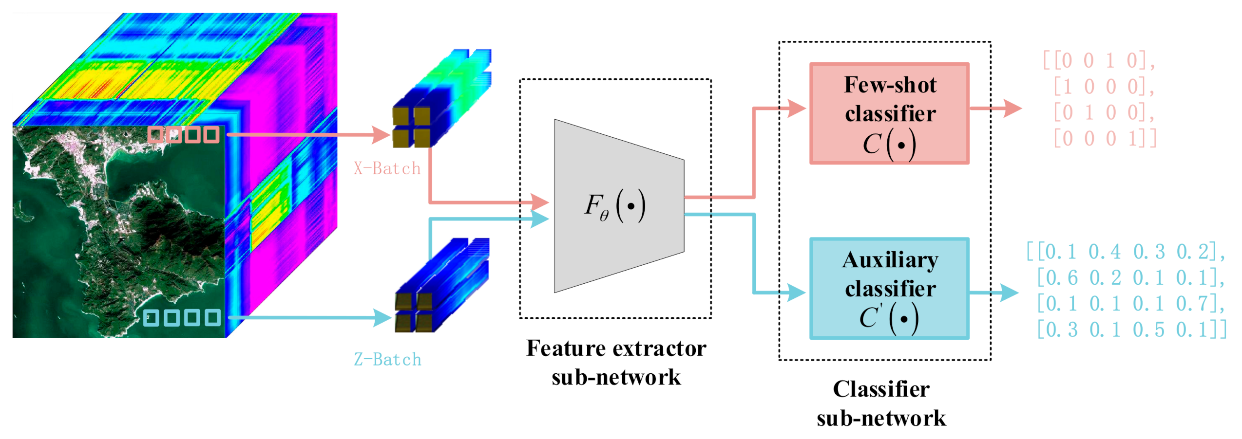
In line with this concept, we propose a two-heads few-shot deep learning framework, illustrated in Figure 1. Two different classifier sub-networks, and separately achieve classification on and , but share a common feature extractor sub-network , denotes the parameters in the feature extractor sub-network. For the classification branch on , the predicted label can be obtained as follows:
where denotes the predicted label for sample . In addition, for the classification branch on , the relationship between the pseudo-label and the sample is formulated as follows:
in which is the predicted label for the unlabeled sample .
We regard four samples as one batch just for convenience, though it is irrelevant to the real settings in experiments. Thanks to the shared feature extractor sub-network, both labeled and unlabeled samples are integrated into one framework, to which more samples are introduced in order to regularize the original few-shot supervised branch. Through joint learning the proposed network via a back-propagation algorithm, the supervision from the auxiliary unlabeled dataset is exploited to appropriately mitigate the overfitting problem resulting from the existence of few labeled samples, i.e., the auxiliary dataset acts as a regularizer that trains the feature extractor. The details of training the proposed model can be seen in Section 2.4.
It is notable that the proposed framework is a general learning framework, through the use of which any kind of deep neural network can be exploited as the feature extractor sub-network. In this paper, we use DCNNs and residual networks, two state-of-the-art network structures, to construct the extraction sub-network. The details are outlined in Section 2.3.
2.2. Soft Pseudo-Label Learning
The proposed framework is trained in a supervised manner using both the labeled and unlabeled samples with pseudo-labels. To achieve this, we require a suitable strategy that assigns a pseudo-label to each unlabeled sample. Some semi-supervised methods conduct clustering (e.g., -means algorithm) on the unlabeled samples to obtain the cluster labels [42], and the cluster labels are then exploited as the pseudo-labels. The -means method can only assign each unlabeled sample a specific unique cluster label that is equivalent to the hard label. For this reason, we use the resulting cluster labels obtained via -means clustering as the hard pseudo-labels. However, this simple strategy has a number of limitations. First, it ignores the relationship between the labeled samples. Second, the hard label cannot adequately represent samples in which the distance to one cluster center is closer than the distances to the other cluster centers. Thus, the classification performance of these methods using hard pseudo-labels is still limited, especially in the few-shot or one-shot setting.
In contrast to hard labels, soft labels have high entropy, and can thus convey more valuable information during the classification process. In addition, soft labels can lead to continuous gradients during network training, which is beneficial for convergence and mitigates the problem of the algorithm becoming trapped into bad local minima [43]. Inspired by this, we propose a soft pseudo-label learning method that operates by exploiting the underlying relation between the labeled and unlabeled sample. In particular, we conclude that specific underlying relations exist such as intra-class similarity and inter-class dissimilarity between the unlabeled sample and the labeled sample. Samples (labeled or not) that belong to the same class show high similarity, while samples (labeled or not) that belong to different classes exhibit obvious difference, and vice versa. Therefore, by considering each labeled sample as a reference agent, we can assign each unlabeled sample a soft pseudo-label by computing the distances between the unlabeled sample and all agents.
In more detail, taking an unlabeled sample as an example, we generate its soft pseudo-label as follows. Firstly, each labeled sample is adopted as an agent, i.e.,
in which denotes the -th training sample from -th class. We then compute the distances between the unlabeled sample and all agents as follows:
Here, is the distance between the agent and the unlabeled sample , which is calculated via the similarity function . For simplicity, we utilize the Euclidean distance as the function , the features used in the function are the original pixel of the HSI. From the distances between and all agents in class , we select the one with the smallest distance as the reference agent in the -th class as follows:
Then, the -th element of pseudo-label can thus be obtained via
By applying the same operations on all classes, the soft pseudo-label of the unlabeled sample can be finally represented as:
It should be noted that all labeled samples of each class are exploited as agents in the proposed method. Although we can average the labeled samples to create a representative agent, this averaging strategy is likely to impair the underlying relation to some extent. For example, some samples are more similar to a specific agent than the average agent, and thus degrade the performance of the proposed method. The experimental results can be seen from the ablation study in Section 3.4.
2.3. The Architecture of the Adopted Feature Extractor Sub-Network and Classifier Sub-Network
Figure 1 illustrates the pipeline of the proposed two-heads few-shot deep learning framework, which includes one shared-feature extractor sub-network, one few-shot classifier sub-network for labeled data, and one auxiliary classifier sub-network for unlabeled data with soft pseudo-labels. Because both labeled and unlabeled data are utilized for training, the proposed method can be seen as a semi-supervised deep learning method. If we utilized a feature extractor sub-network and a few-shot classifier sub-network only within the proposed framework, the proposed framework would degenerate into a standardly used supervised deep learning method. Thus, by comparing the proposed method with its supervised counterpart (i.e., utilizing the feature extractor sub-network and few-shot classifier sub-network only), the advantage of introducing unlabeled data for HSI classification can be observed. For this reason, we refer to the supervised counterpart as the backbone. It is notable that the proposed network is a two-head network structure, while its supervised counterpart is a one-head network structure (with a few-shot classifier sub-network, but without an auxiliary classifier sub-network).
The proposed framework is a general learning framework, which enables any kind of deep neural network to be exploited as the feature extractor sub-network. In various applications, to demonstrate the adaptability of the proposed framework to different network structures, two network structures that are widely used for HSI classification (i.e., 3D-CNN and SSRN) are adopted as the feature extraction sub-network. It is notable that the structure of the classifier sub-network (i.e., the heads) is fixed because it is rather simple (i.e., the classifier sub-network is implemented via a fully connected layer).
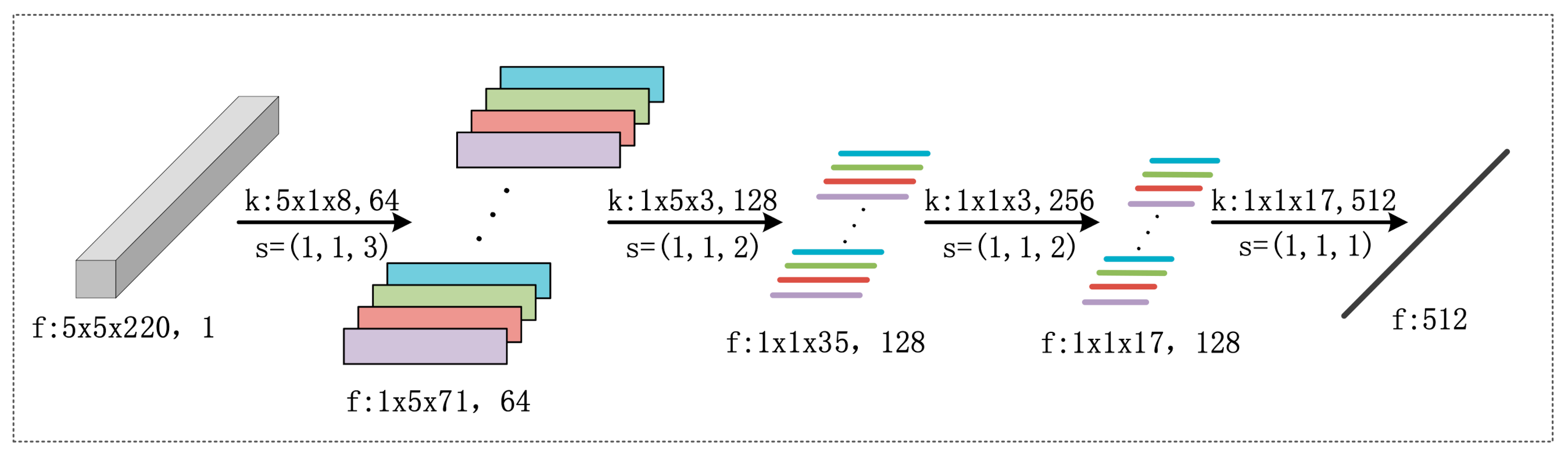
(1) 3D-CNN feature extractor sub-network: It has been demonstrated that a 3D-CNN structure that utilizes both spatial and spectral information can result in better HSI classification performance when compared with a method which utilizes only the spectrum information. This is because HSI data is inherently a 3D data cube that contains both spatial and spectral information, which makes 3D-CNN a natural structure choice. Thus, 3D-CNN is adopted as the first backbone network for feature extraction. By following the settings of existing 3D-CNN structures for HSI classification, we constructed a 3D-CNN network for feature extraction, as illustrated in Figure 2. The network consists of four convolutional layers, each of which is equipped with 3D convolutional kernels for feature extraction. The detailed parameter settings (such as convolution kernels and stride) are also included in Figure 2. The network contains 3 convolutional layers and a fully connected layer. In the first convolutional layer, the kernel size is 5 × 1 × 8 and 64 feature maps; in the second convolutional layer, the kernel size is 1 × 5 × 3 and 128 feature maps; in the third convolutional layer, the kernel size is 1 × 1 × 3 and 256 feature maps, s is the step size. The finally fully connected layer includes 512 nodes.
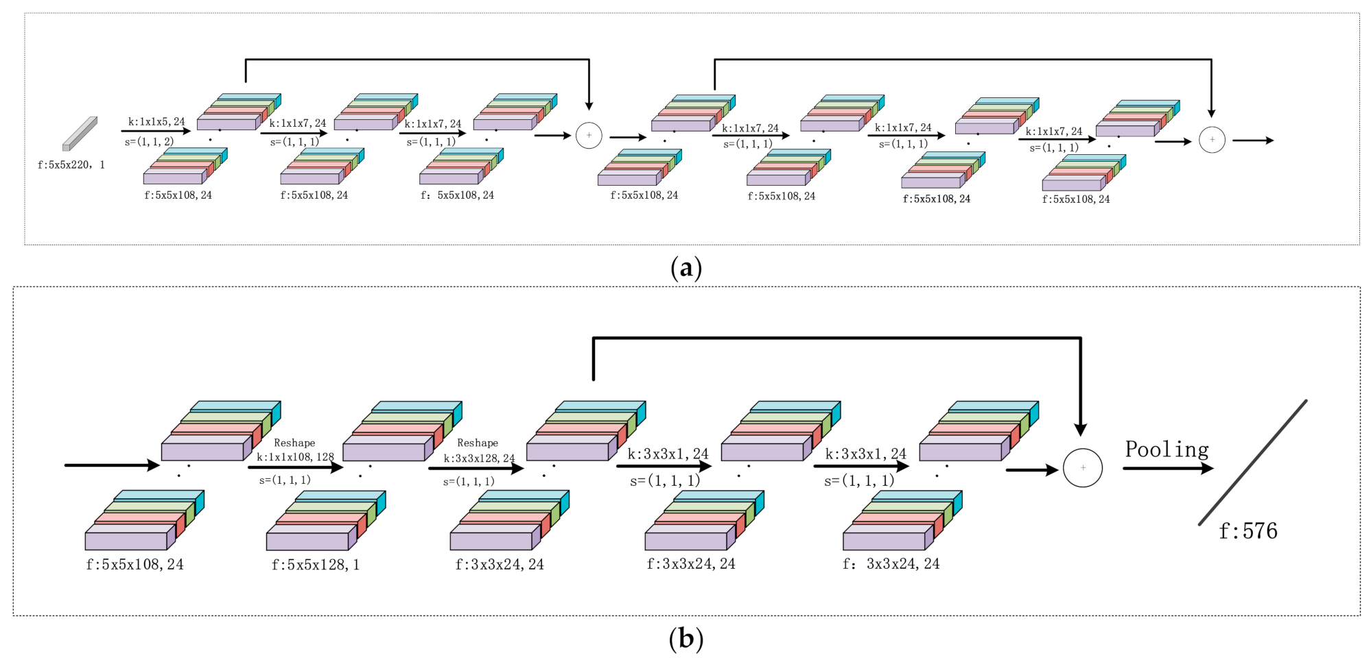
(2) SSRN feature extractor sub-network: Although DCNN has a strong feature extraction ability, due to the gradient vanishing problem it becomes difficult to train a deep neural network as the network depth increases. To overcome the gradient vanishing problem due to increasing network depth, He et al. propose a novel residual learning structure that can successfully mitigate the gradient vanishing problem [24]. The key to residual learning is to introduce a shortcut connection into the original network structure, with which the gradient vanishing problem can be well mitigated. Inspired by this, many recent HSI classification methods have also begun to take advantage of residual learning to train a deeper neural network. For this purpose, SSRN, a typical residual learning structure-based network, is exploited as the feature extractor sub-network within the proposed network. More specifically, we constructed a spectral-spatial residual network to capture both the spectral and spatial information. In this network, the spectral and spatial information is extracted consecutively based on the spectral and spatial residual blocks. For the spectral residual learning block, the convolutional layers, together with two shortcut connections, are utilized to extract the spectral features. For the spatial residual learning block, the convolutional layers, together with one shortcut connection, are exploited to extract spatial information. The details of the modeled residual network can be seen in Figure 3, which also includes the architecture and the parameter settings.
(3) Classifier sub-network: In general, the classifier sub-network adopts a much simpler architecture when compared with the feature extractor sub-network above. For the supervised deep learning-based classification task, it often consists of a fully connected layer. In this study, we use two fully connected layers to form the classifier sub-networks on and independently.
2.4. Loss Function
The constructed deep neural network contains a number of unknown parameters. To train and determine those parameters using a back-propagation algorithm, an appropriate loss needs to be defined beforehand.
Since the proposed network is a two-branch network, which includes two separate classification tasks on and , for the classification branch on , we adopt the cross-entropy loss, defined as follows:
Here, is an -dimensional vector calculated via Equation (1), which predicts the label of .
It is notable that this achieves a classification task with very limited labeled samples. However, a deep neural network with a large number of parameters will confront a heavily ill-posed problem when provided with few labeled training samples (e.g., five samples per class) for an HSI classification task. This is primarily because a large number of parameters cannot be fully and directly trained with a small number of labeled training samples; i.e., the parameters obtained by optimizing Equation (8) are unstable.
To resolve this issue, an effective method in the machine learning field is to enforce a suitable regularization item into Equation (8), from which the solution space can be effectively reduced to find a stable parameter. Inspired by this, we propose utilizing the unlabeled data with soft labels (i.e., the classification task on the auxiliary dataset ) as the regularization item, as follows:
where is an -dimensional vector calculated by Equation (2).
With these two loss functions defined above, we can formulate the overall loss function of the proposed two-branch network as follows:
where is a predefined weighting factor. It is notable that the shared feature extractor module can guarantee these two branches are trained jointly. Then, by minimizing the loss , the parameters can be trained with the back-propagation algorithm.
3. Experiments
To demonstrate the effectiveness of the proposed method in terms of few-shot HSI classification, we conducted experiments on three benchmark HSI datasets. In the below, we will first introduce the adopted benchmark HSI datasets and the experimental settings. We will next explain the undertaken appropriate and adequate comparison experiments between the proposed method and some state-of-the-art HSI classification methods in various cases, followed by some ablation studies.
3.1. Datasets
In this study, three benchmark HSI datasets were adopted to verify the efficacy of the proposed method including the Pavia University (PaviaU) dataset, the Salinas dataset, and the Indian Pines dataset [44].
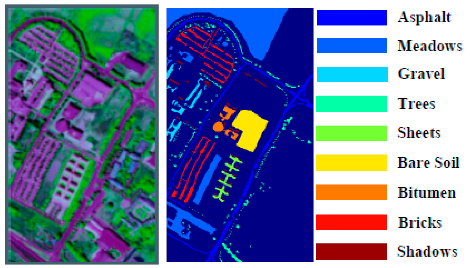
PaviaU dataset: The PaviaU dataset was acquired by a sensor during a flight campaign over the university of Pavia, Italy, and includes 9 classes and pixels, as shown in Table 1. In addition, the false color image and the ground truth map are shown in Figure 4. For the PaviaU dataset, each pixel has 103 spectral reflectance bands ranging from 430 to 860 nm, and the spatial resolution is 1.3 m. In these experiments, all bands are utilized for HSI classification.
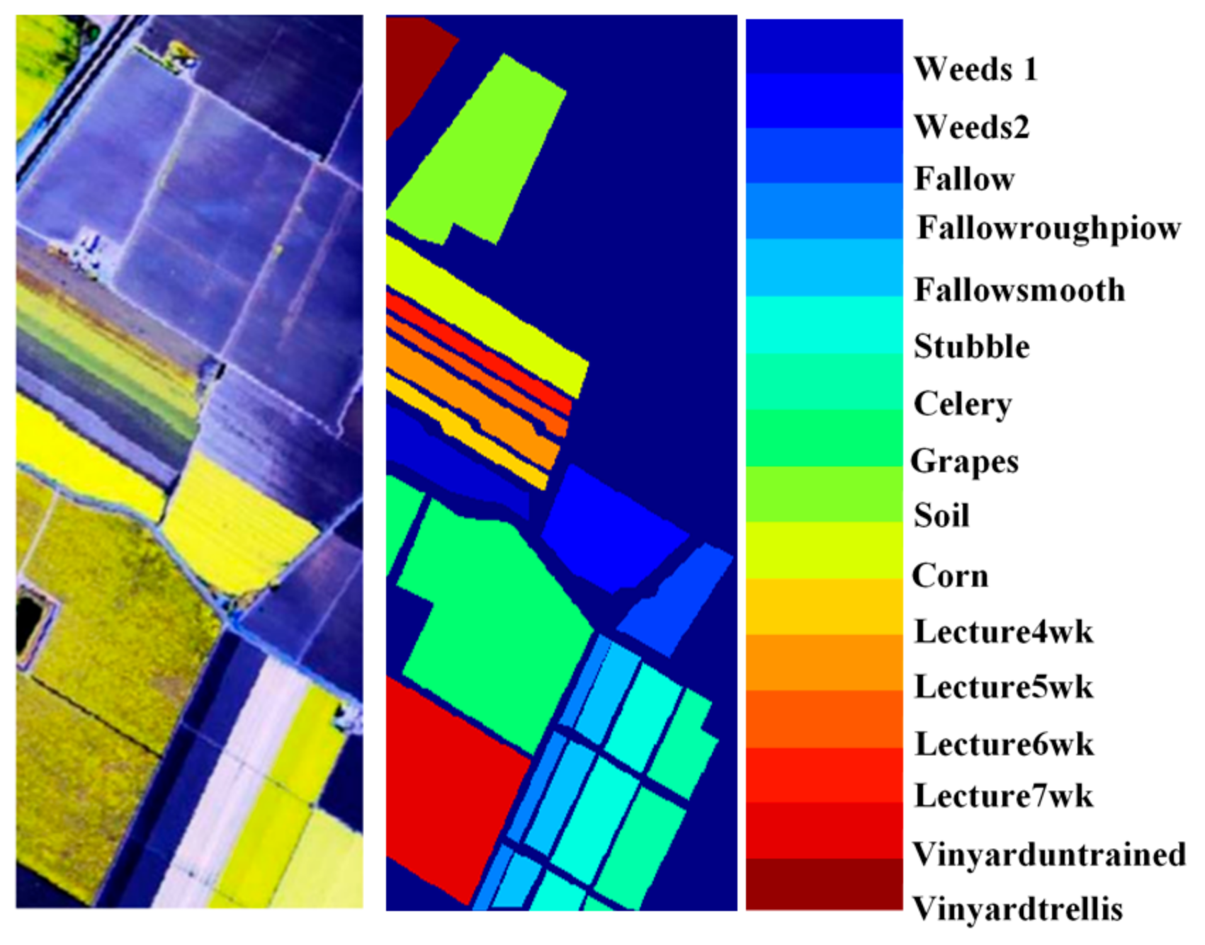
Salinas dataset: The Salinas dataset was acquired using the Airborne Visible/Infrared Imaging Spectrometer (AVIRIS) from California, which includes 16 classes and pixels (shown in Table 1). The spatial resolution is 3.7 m. The false color image and the ground truth map are shown in Figure 5. For this dataset, each pixel has 224 bands ranging from 400 to 2450 nm. After the water-absorption bands were removed, 204 bands were retained for the experiments.
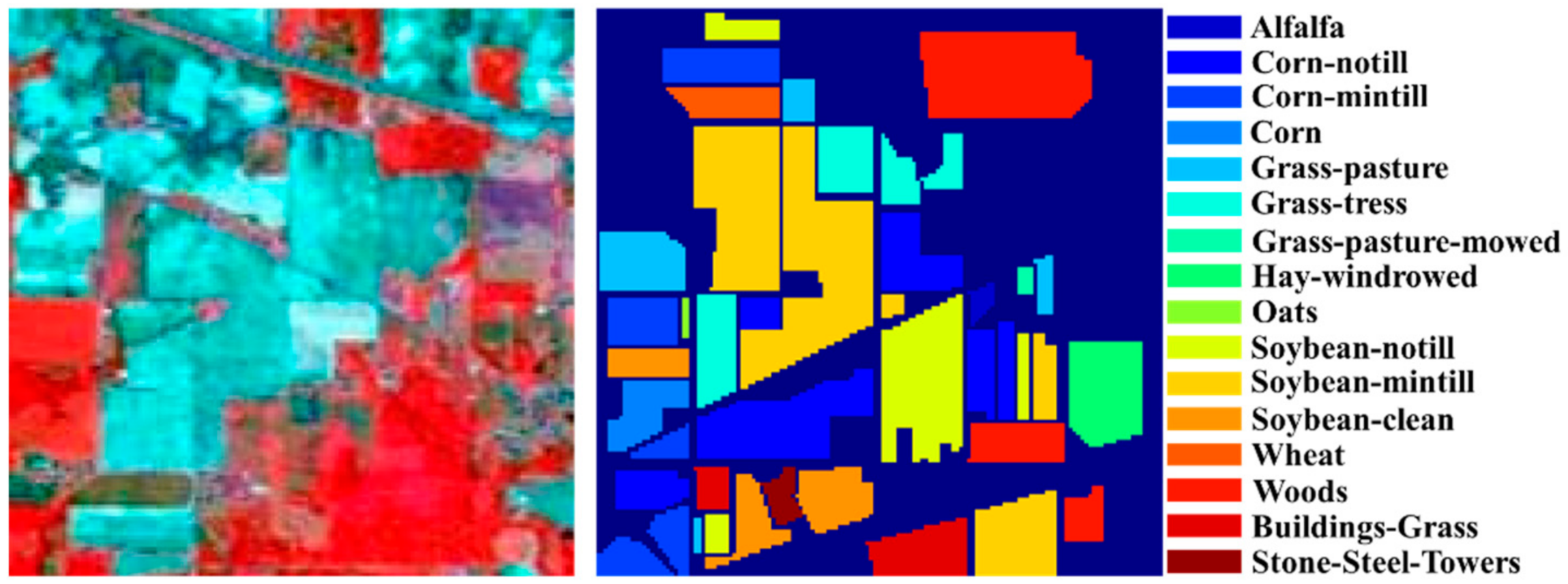
Indian Pines dataset: The Indian Pines dataset was collected by AVIRIS from the agricultural Indiana Pines test site in northwestern Indiana. It contains 16 land cover classes and images of pixels. The detailed class name, the numbers of labeled pixels and the class map can be seen in Table 1 and Figure 6. The spatial resolution of HSI in this dataset is about 20 m. Each pixel has 220 spectral reflectance bands ranging from 400 to 2450 nm. All 220 bands were utilized for HSI classification in this experiment.
These three datasets have a public characteristic, which are all unbalanced datasets.
3.2. Comparison Methods and Measures
To verify the performance of the proposed method, we compared it with Support Vector Machine (SVM), Spatio-Spectral Laplacian Support Vector Machine (SS-LapSVM) [37], 3D-GAN [39], SS-CNN [38], 3D-CNN, SSRN [26], and 3D Densely Connected Convolutional Network (3D-Densenet) [25]-based HSI classification methods. Among these competing methods, the SVM-based method is a conventional machine learning-based method that specializes in dealing with small sample problems. SS-LapSVM is a traditional semi-supervised method that utilizes both labeled and unlabeled samples. 3D-GAN and SS-CNN are deep learning-based methods for semi-supervised HSI classification. 3D-CNN and SSRN are two representative deep learning-based methods, which utilize the labeled samples only for classification and also serve as the backbone for feature extraction. Based on these two backbone feature extractor networks, we obtained two different versions of the proposed method. For the sake of simplicity, we denote the proposed method based on 3D-CNN and SSRN as and , respectively. To facilitate further comparison, variants of the proposed two-branch networks were specifically designed so that only the soft pseudo-labels are replaced by the hard pseudo-labels generated via k-means clustering [42]. We denote these two variant methods as and . For the adopted k-means clustering method, the number of clusters is set equal to the categories within the HSI dataset (e.g., we set the number of clusters to 16, since there are 16 categories in the Indian Pines dataset). To further testify the effectiveness of proposed soft pseudo-labels, we generate the hard label via the proposed soft pseudo-label learning method, in which one sample can only belong to one category. The proposed method with hard pseudo-label is denoted as and . In addition, 3D-Densenet, a newly proposed deep learning-based method that achieves excellent HSI classification performance when provided with plenty of labeled samples was also introduced as a competing method.
As for the evaluation measurement, three conventional evaluation metrics including overall accuracy (OA), average accuracy (AA) and the Kappa coefficient were adopted to evaluate the HSI classification performance of different methods.
3.3. Experimental Results
In this subsection, we focus primarily on comparing the proposed method with other competing methods in order to demonstrate its effectiveness in the field of HSI classification under few-shot and one-shot settings. Since the problem we are addressing involves obtaining an appropriate deep learning-based method when heavily limited labeled samples are provided for training, we conducted experiments with three and five labeled samples per class and experiments with one labeled sample per class. In more detail, the experiments with three and five labeled samples per class correspond to the few-shot HSI classification problem, while the experiments with one labeled sample are for a more challenging one-shot HSI classification task.
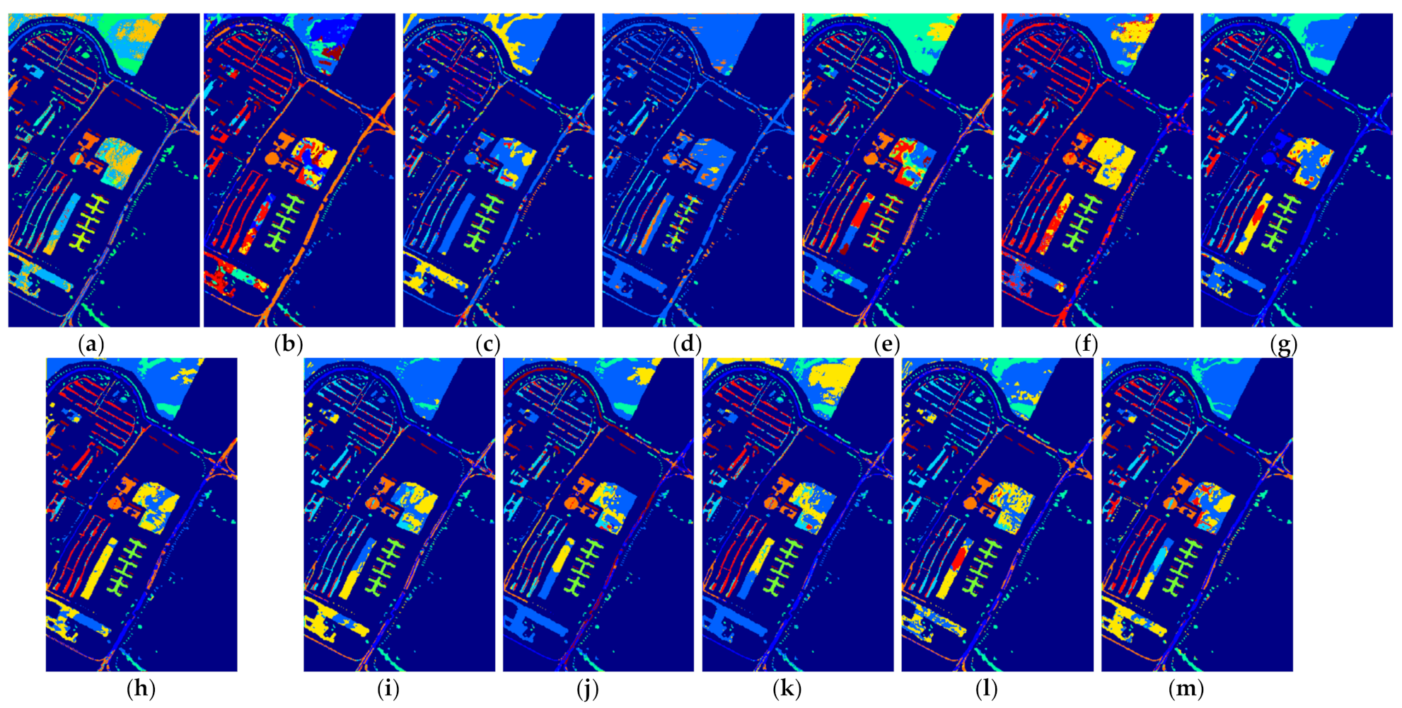
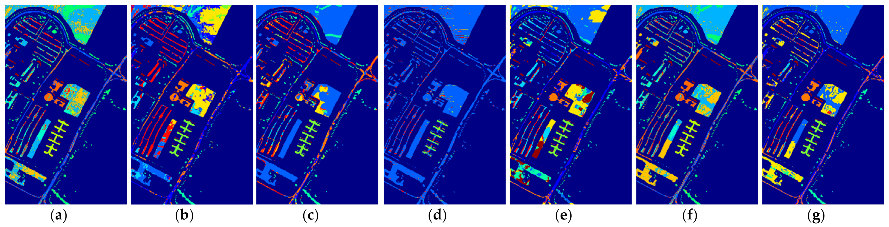
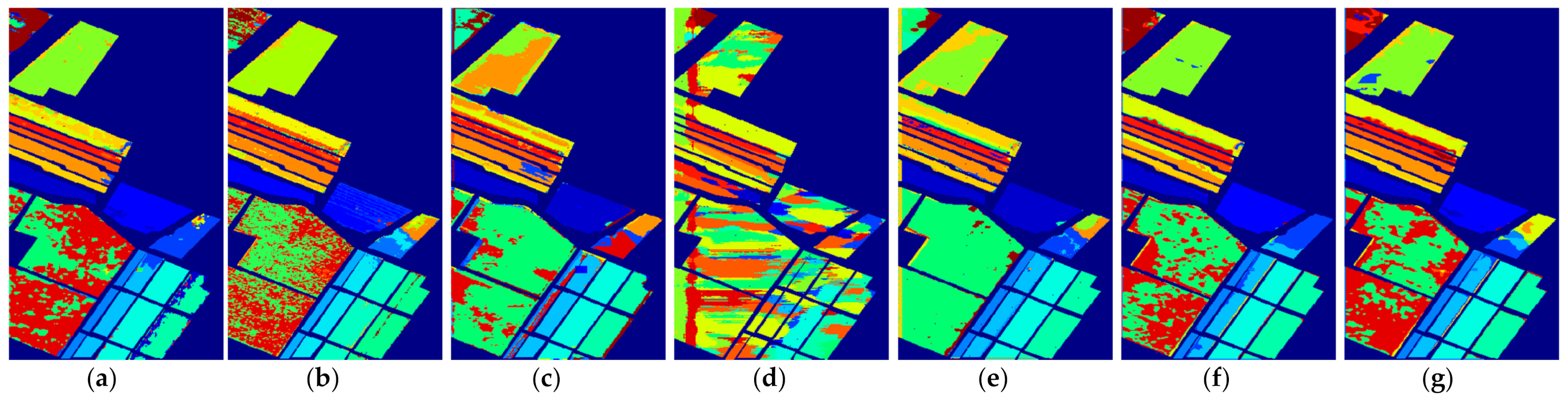
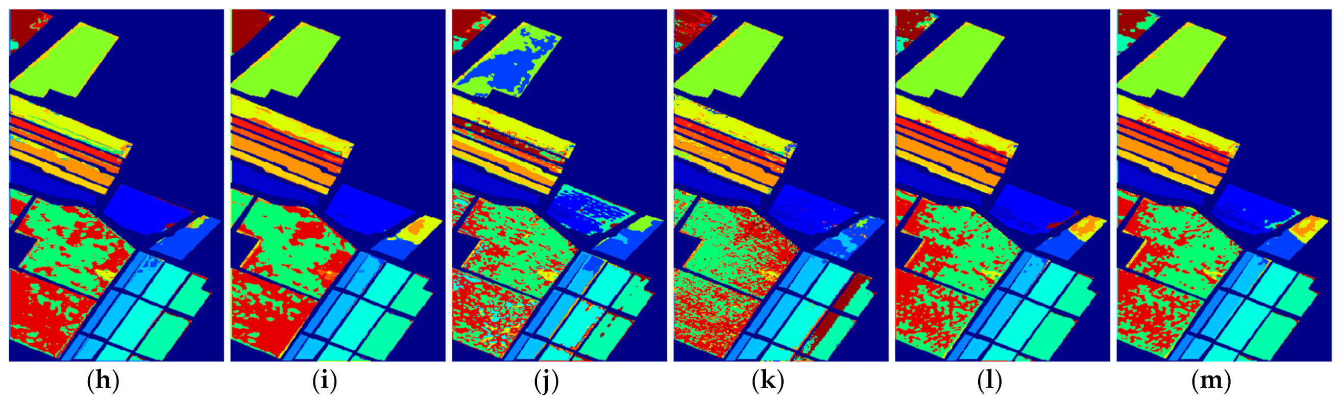
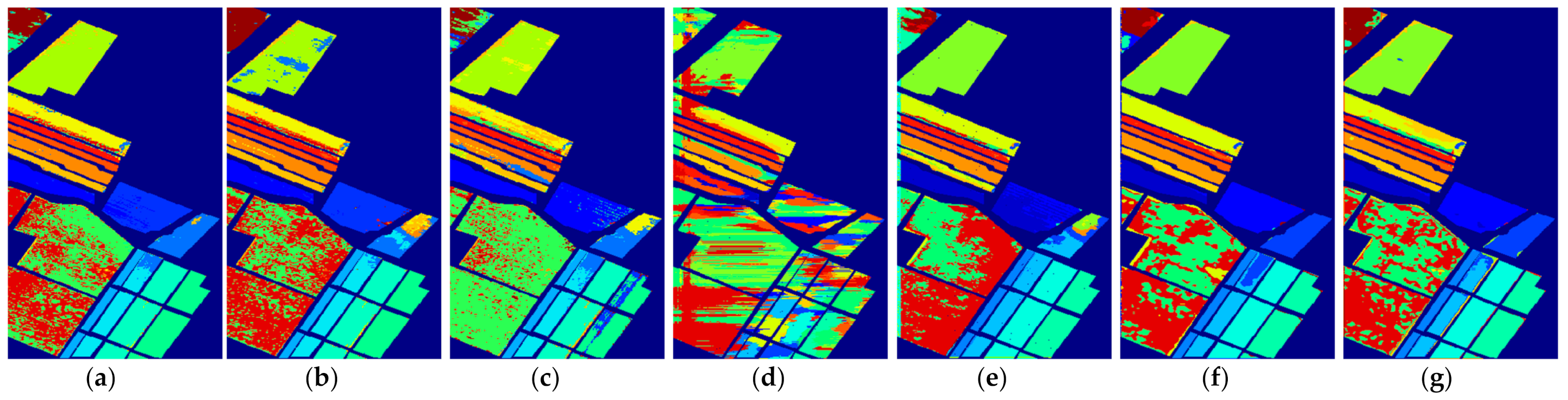
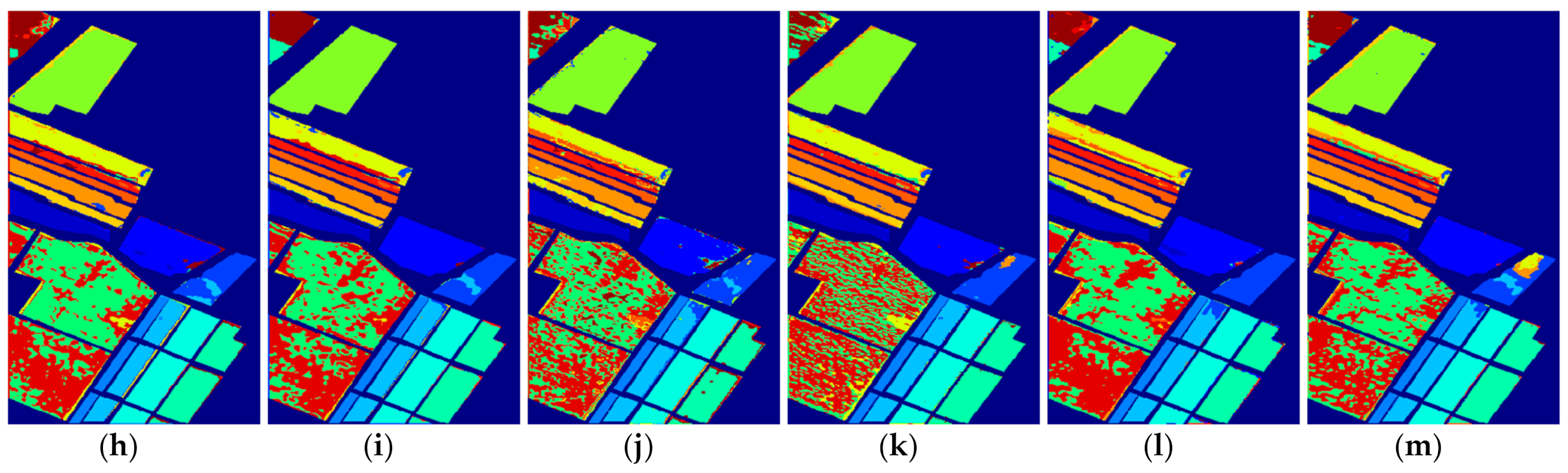
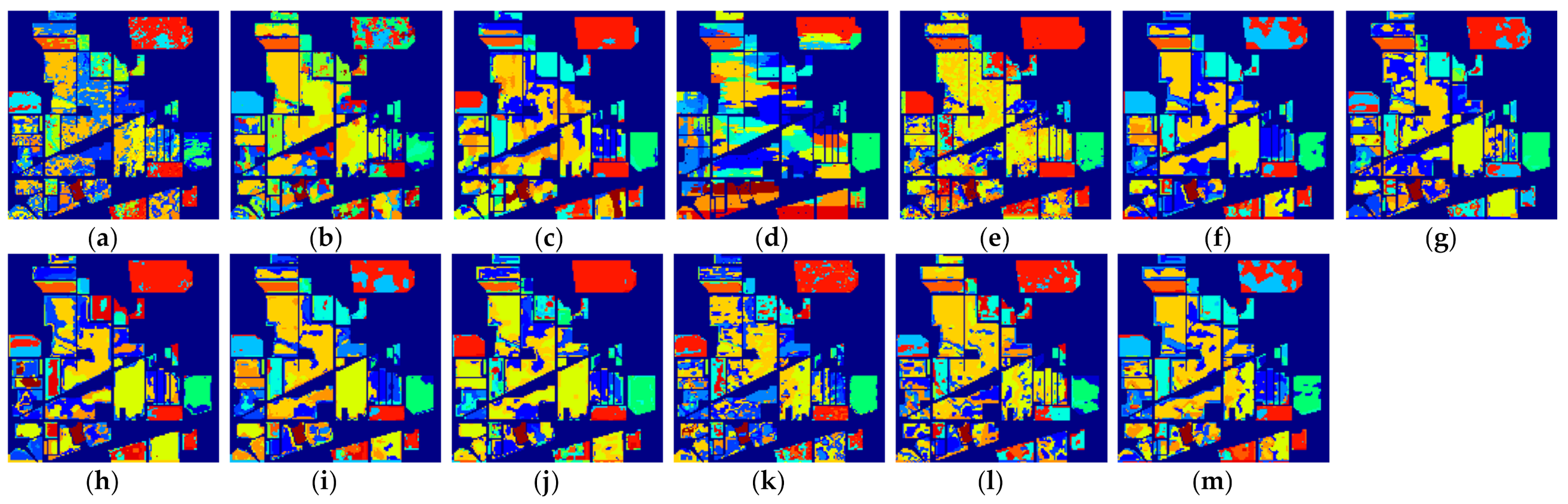
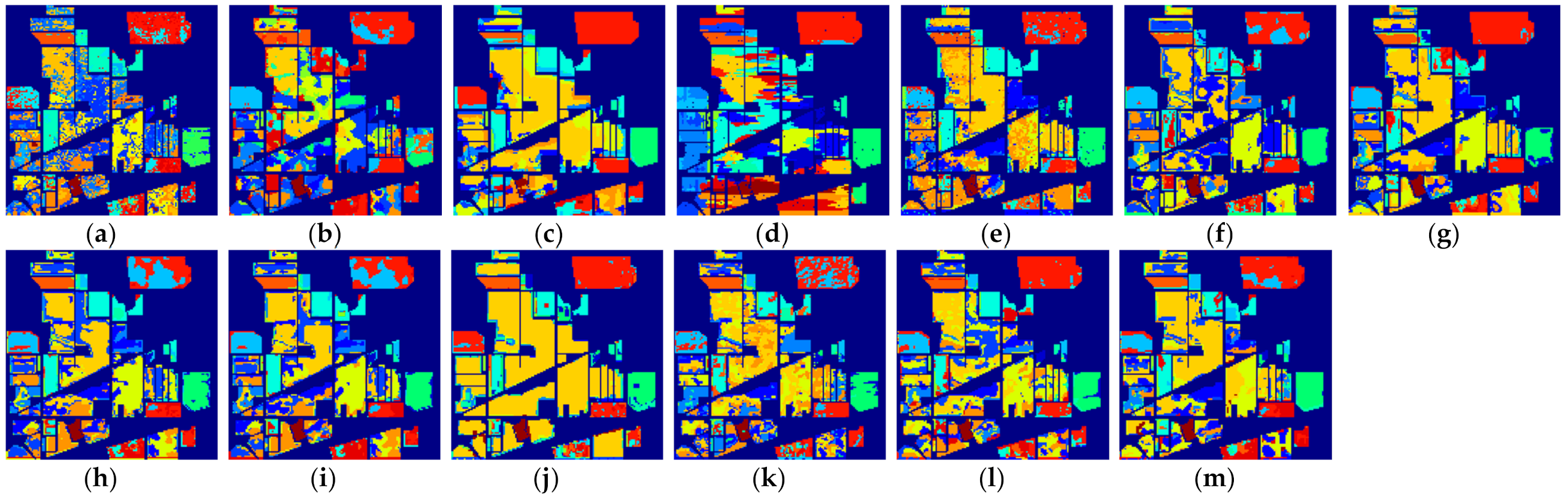
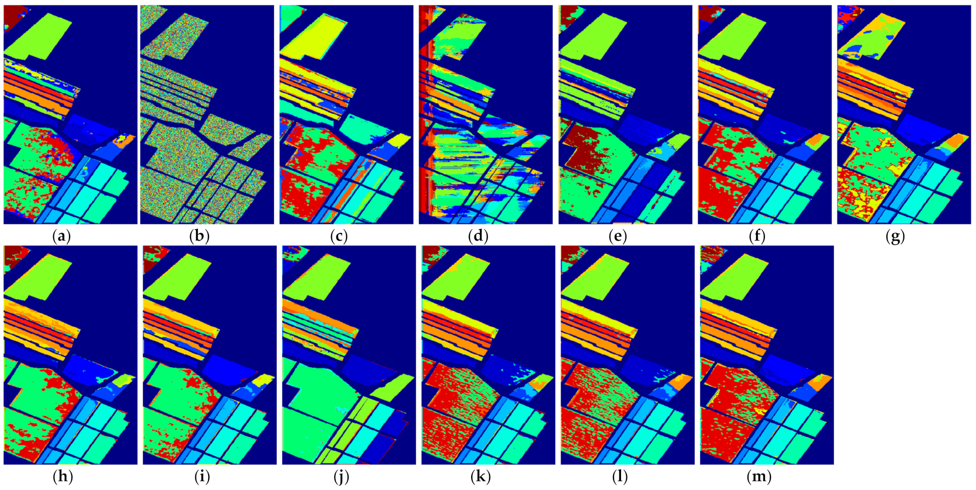
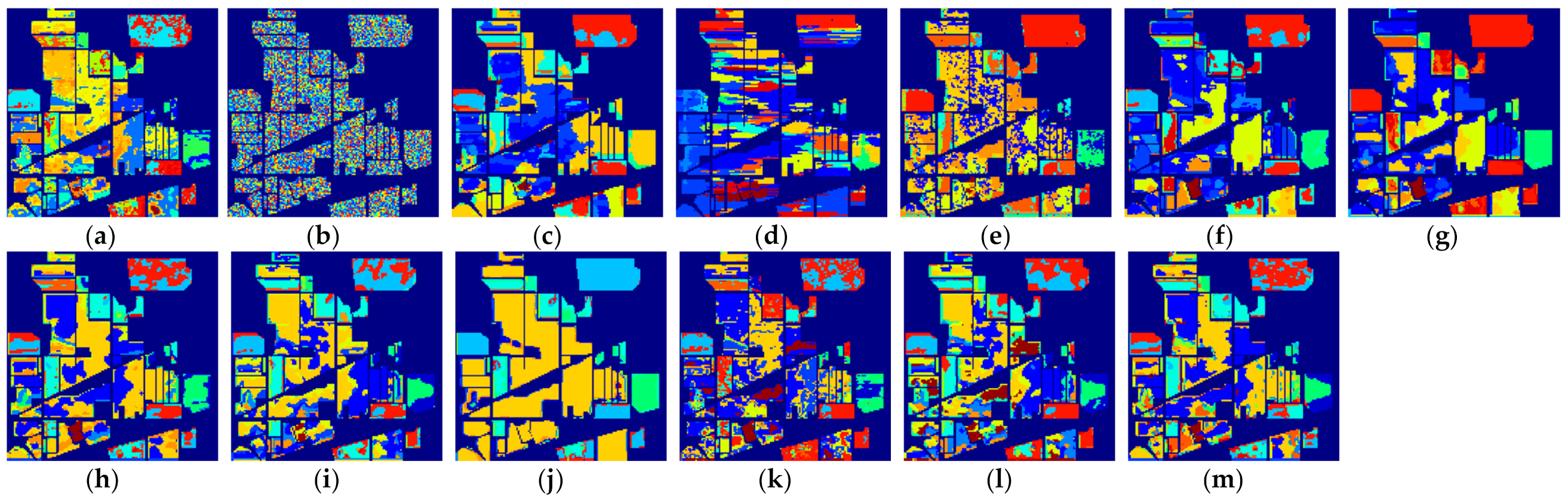
We repeated the same HSI classification process for each number of labeled samples. Taking three labeled samples as an example, we randomly chose three labeled samples per class as the training set, then treated the rest of the samples as the test set in the classification experiments. To eliminate the influence of randomness on classification accuracy when selecting training samples, the final classification accuracy for each method was calculated by averaging the classification results independently obtained from ten random training and testing rounds. The average classification results for all methods on different datasets are summarized and reported in Table 2, Table 3, Table 4, Table 5, Table 6, Table 7, Table 8, Table 9 and Table 10. To more accurately assess the performance of the different methods, the classification maps of these methods on three datasets are also visualized in Figure 7, Figure 8, Figure 9, Figure 10, Figure 11, Figure 12, Figure 13, Figure 14 and Figure 15, where (a)–(m) represent the results from different classification methods. From these listed results, we obtained the following conclusions.
(1) Comparison with conventional machine learning-based method: Although the effectiveness of the deep learning-based methods has been demonstrated when a large number of labeled samples are provided for training, it can be seen from the results in Table 2 that the performance of the deep learning-based methods cannot be guaranteed when only a few labeled samples are provided. In most cases, the performance of 3D-Densenet and are even inferior to that of SVM. This is because deep structured network-based methods are prone to overfitting when few labeled training samples are provided. Nevertheless, the proposed deep learning methods obtain better performance in the majority of cases than SVM. For example, the proposed method improves OA over SVM by about 5.52% when five labeled samples in PaviaU dataset are provided, which demonstrates that the proposed networks can better adapt to the few-shot HSI classification problem.
(2) Comparison with semi-supervised method: In all methods, SS-LapSVM, 3D-GAN, SS-CNN, the proposed methods (i.e., and ), two variants of our methods (including and ), and the proposed method with hard pseudo-label (including and ) are semi-supervised methods. From the results, we can observe that the proposed methods have obvious advantages over the competing semi-supervised methods in terms of HSI classification when only a very limited number of training samples are provided for training. It is notable that the traditional semi-supervised method SS-LapSVM achieves almost the worst performance out of all comparison methods. Compared with deep learning-based semi-supervised methods such as 3D-GAN and SS-CNN, the proposed method (i.e., ) shows promising results with a higher accuracy. Considering all these methods are semi-supervised methods, we can conclude that the proposed method can better utilize the unlabeled data for better HSI classification results. In addition, by comparing the performance of the proposed methods with and as well as and , we can see that the soft pseudo-labels also contribute to the improvement of HSI classification.
(3) Comparison with deep learning-based method: 3D-Densenet, 3D-CNN, SSRN, the proposed methods ( and ) and the two variants of the proposed methods ( and ) are all deep learning-based methods. From the results, we can see that the proposed methods achieve better classification performance than other competing deep learning-based methods. This is because the competing methods, such as 3D-Densenet, are more likely to be overfitting when heavily few-labeled samples are available for HSI classification. By contrast, with the regularization from the auxiliary dataset with soft pseudo-labels, the overfitting problem of the proposed method can be effectively reduced, with which the classification accuracy is improved.
(4) Applicability to different kinds of networks: The proposed framework is a general semi-supervised framework, with which the unlabeled samples could be effectively used to mitigate overfitting and improve the HSI classification accuracy. To demonstrate the applicability of the proposed framework to different kinds of networks, we used a 3D-CNN and SSRN as the backbones (i.e., only utilizing the labeled samples for training). By comparing the results between (i.e., the proposed method) and 3D-CNN, we can find that the proposed method based on the structure could obtain better performance on three datasets with different number of training samples. For example, when provided five labeled training samples on the PaviaU dataset, the average OA of is improved by 3.89% over 3D-CNN. Similar, the experimental results from SSRN and also reflect that the obtains better classification results. In summary, from the results of both 3D-CNN and SSRN, we can conclude that the proposed framework is applicable to different kinds of networks for few-shot learning.
(5) Applicability to one-shot HSI classification: The proposed methods do not only improve the few-shot HSI classification with heavily limited training samples (i.e., three and five labeled samples), but can also improve the one-shot HSI classification when only one training sample per class is provided. Although the performance from the one-shot classification cannot be compared with that of the few-shot classification for all methods, it can be observed in Table 8 that the proposed methods still achieve better performance relative to the other comparison methods. For example, the proposed method outperforms SVM by 8.68% in terms of OA on the Indian Pines dataset. In addition, it can be observed that when only one labeled sample is provided, the SS-LapSVM method even fails to classify the test samples in these benchmark datasets, which indicates the difficulty of utilizing the unlabeled samples with only one labeled training sample. Nevertheless, the proposed method effectively utilizes the unlabeled samples and thus yields better classification results. We can therefore conclude that the proposed method is also effective for one-shot classification.
3.4. Ablation Study
(1) Effectiveness of the reference agent: In this paper, a group of agent references were adopted to assign soft pseudo-labels, among which all labeled samples of each class were exploited as agents. In addition to this strategy, we also average all labeled samples to generate a representative agent for each class, then utilized the representative agent to obtain the soft pseudo-label, which is referred to as Average in this study. To demonstrate the superiority of the proposed agent learning method, we conducted comparison experiments between Ours and Average. Table 11 reports the comparison results, in which 3D-CNN was adopted as the backbone and five labeled samples were provided for training. It can thus be seen that the performance of Ours achieves promising results with a higher accuracy than that of Average, as shown in Table 11. For example, the OA of Ours outperforms Average by 1.45%. This is because the underlying relation is impaired to some extent when averaging all labeled samples of each class, whereas the method we adopt preserves these relations.
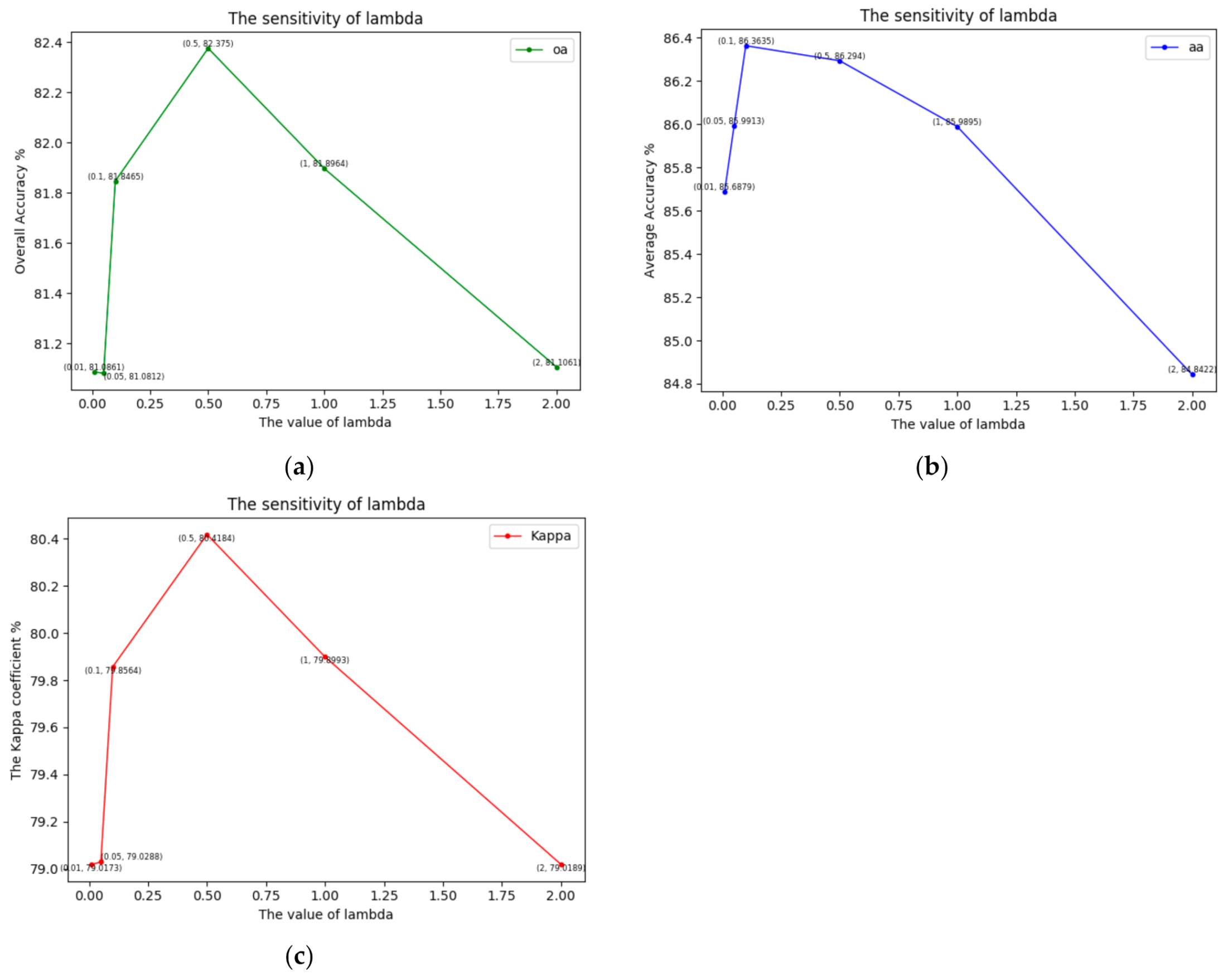
(2) Sensitivity of : We used the loss function defined in Equation (10) to train and determine the parameters contained in the proposed two-branch deep neural network, where was used to balance the loss function from each branch. Figure 16 illustrates the performance of OA, AA and the Kappa coefficient κ as it varies with different , in which the OA, AA and the Kappa coefficient are average results from 10 rounds of experiments with the 3D-CNNours feature extractor, trained with three labeled samples. From the results, we can determine that the classification performance of the proposed method first increases and then decreases as increases from 0 to 2. When λ is around 0.5, the proposed method can obtain its best performance.
(3) The impact of feature extraction: According to the proposed framework, the features were automatically extracted from the data since the proposed method is an end-to-end deep learning-based method. To verify that the proposed network may also be utilized with other feature extraction methods (i.e., we input the extracted feature rather than the original data into the constructed network), we utilized a commonly used feature extraction method termed principal component analysis (PCA) for experiments. More specifically, we extract the PCA features from the original spectrum for each pixel, then input the PCA feature instead of the original spectrum into the constructed two-head network. The results are summarized in the following Table 12. It can be seen that the proposed method still achieves better performance when input with PCA features.
(4) Effectiveness of the two-head network: To demonstrate the effectiveness of the constructed two-head network, we constructed a one-head network structure which includes only the shared feature extraction module and one classification module. Both labeled data (with true-class label) and un-labeled data (with pseudo-label) were trained with the same network structure. In this case, the only difference between the proposed method and this competing method is that the proposed method utilizes a two-branch network structure while the competing method utilizes a one-branch network. Results from the experiments conducted on the PaviaU dataset are summarized in Table 13. It can be clearly seen that the constructed two-head network obtains better performance compared with the one-head structure-based method in most cases, to which we can attribute the improvement of the proposed method over one-head 3D-CNN to the two-branch strategy.
(5) Effect of the proposed pseudo-label generation method: To further verify the effectiveness of the adopted soft pseudo-label generation method based on reference agent, we further conducted a comparison method, in which only the soft pseudo-labels were generated based on the k-means method. Specifically, we first run -means to get the cluster centers, and then utilized the distances between the unlabeled data and the cluster centers to compute the soft-labels for the unlabeled data. The relative experiments are summarized in Table 14. It can be clearly seen that the proposed pseudo-label generation method based on a reference agent has better performance compared with the pseudo-label generation method based on -means.
4. Conclusions
The training process of deep neural networks usually depends on the availability of a large number of training labeled samples. However, owing to the heavy labeling cost for HSI data, the number of labeled samples available in practical applications is heavily limited, resulting in the deep neural network-based HSI classification method overfitting and achieving a poor generalization ability. To address this issue, this paper has proposed a novel few-shot learning method for HSI classification, which borrows the supervision from the auxiliary dataset with soft pseudo-labels in order to train the feature extractor on the few-shot dataset. By employing joint training on both a few-shot dataset and auxiliary dataset with soft pseudo-labels, the proposed method can achieve better classification results on both few-shot HSI classification and one-shot HSI classification tasks. Experimental results demonstrate the superiority of the proposed approach on three hyperspectral benchmark datasets, compared with other competing methods.
Author Contributions
All of the authors made significant contributions to this work. C.D., W.W. and L.Z. devised the approach and analyzed the data; L.Z., Y.Z. and W.W. helped design the remote sensing experiments and provided advice for the preparation and revision of the work; and Y.L., Y.W. and M.Z. performed the experiments. All authors have read and agreed to the published version of the manuscript.
Funding
This work was supported by the National Natural Science Foundations of China (Grant no.61901369 and Grant no.62071387), the Foundation of National Engineering Laboratory for Integrated Aero-Space-Ground-Ocean Big Data Application Technology (Grant No.20200203) and the National Key Research and Development Project of China (No. 2020AAA0104603).
Data Availability Statement
Not applicable.
Acknowledgments
The paper is funded by the key discipline special fund construction project of Shaanxi Province. We acknowledge the author for the HSI datasets.
Conflicts of Interest
The authors declare no conflict of interest.
References
- Ghamisi, P.; Yokoya, N.; Li, J.; Liao, W.; Liu, S.; Plaza, J.; Rasti, B.; Plaza, A. Advances in Hyperspectral Image and Signal Processing: A Comprehensive Overview of the State of the Art. IEEE Geosci. Remote Sens. Mag. 2017, 5, 37–78. [Google Scholar] [CrossRef] [Green Version]
- Wei, W.; Zhang, L.; Jiao, Y.; Tian, C.; Wang, C.; Zhang, Y. Intracluster Structured Low-Rank Matrix Analysis Method for Hyperspectral Denoising. IEEE Trans. Geosci. Remote Sens. 2018, 57, 866–880. [Google Scholar] [CrossRef]
- He, L.; Li, J.; Liu, C.; Li, S. Recent Advances on Spectral-Spatial Hyperspectral Image Classification: An Overview and New guidelines. IEEE Trans. Geosci. Remote Sens. 2017, 56, 1579–1597. [Google Scholar] [CrossRef]
- Guerra, R.; Barrios, Y.; Díaz, M.; Santos, L.; López, S.; Sarmiento, R. A new algorithm for the on-board compression of hyperspectral images. Remote Sens. 2018, 10, 428. [Google Scholar] [CrossRef] [Green Version]
- Zhang, L.; Wei, W.; Bai, C.; Gao, Y.; Zhang, Y. Exploiting Clustering Manifold Structure for Hyperspectral Imagery Super-Resolution. IEEE Trans. Image Process. 2018, 27, 5969–5982. [Google Scholar] [CrossRef] [PubMed]
- Weiss, M.; Jacob, F.; Duveiller, G. Remote sensing for agricultural applications: A meta-review. Remote Sens. Environ. 2020, 236, 111402. [Google Scholar] [CrossRef]
- Tu, B.; Wang, J.; Kang, X.; Zhang, G.; Ou, X.; Guo, L. KNN-Based Representation of Superpixels for Hyperspectral Image Classification. IEEE J. Sel. Top. Appl. Earth Obs. Remote Sens. 2018, 11, 4032–4047. [Google Scholar] [CrossRef]
- Andriyanov, N.; Dementiev, V.; Kondratiev, D. Tracking of Objects in Video Sequences. Intell. Decis. Technol. 2021, 253–262. [Google Scholar]
- Andriyanov, N.A.; Vasil’ev, K.K.; Dement’ev, V.E. Investigation of Filtering and Objects Detection Algorithms for A Multizone Image Sequence. Int. Arch. Photogramm. Remote Sens. Spat. Inf. Sci. 2019, 4, 7–10. [Google Scholar] [CrossRef] [Green Version]
- Hu, H.; Gu, J.; Zhang, Z.; Dai, J.; Wei, Y. Relation Networks for Object Detection. In Proceedings of the 2018 IEEE/CVF Conference on Computer Vision and Pattern Recognition, Salt Lake City, UT, USA, 18–23 June 2018; pp. 3588–3597. [Google Scholar]
- Cai, Z.; Vasconcelos, N. Cascade R-CNN: Delving Into High Quality Object Detection. In Proceedings of the 2018 IEEE/CVF Conference on Computer Vision and Pattern Recognition, Salt Lake City, UT, USA, 18–23 June 2018; pp. 6154–6162. [Google Scholar]
- Chen, L.-C.; Zhu, Y.; Papandreou, G.; Schroff, F.; Adam, H. Encoder-Decoder with Atrous Separable Convolution for Semantic Image Segmentation. In Proceedings of the European Conference on Computer Vision (ECCV), Munich, Germany, 8–14 September 2018; pp. 833–851. [Google Scholar]
- Wang, P.; Chen, P.; Yuan, Y.; Liu, D.; Huang, Z.; Hou, X.; Cottrell, G. Understanding Convolution for Semantic Segmentation. In Proceedings of the 2018 IEEE Winter Conference on Applications of Computer Vision (WACV), Lake Tahoe, NV, USA, 12–15 March 2018; pp. 1451–1460. [Google Scholar]
- Zhang, H.; Dana, K.; Shi, J.; Zhang, Z.; Wang, X.; Tyagi, A.; Agrawal, A. Context Encoding for Semantic Segmentation. In Proceedings of the IEEE Conference on Computer Vision and Pattern Recognition (CVPR), Salt Lake City, UT, USA, 18–23 June 2018; pp. 7151–7160. [Google Scholar]
- Yalniz, I.Z.; Jégou, H.; Chen, K.; Paluri, M.; Mahajan, D. Billion-scale semi-supervised learning for image classification. arXiv 2019, arXiv:1905.00546. [Google Scholar]
- Liang, P.; Shi, W.; Zhang, X. Remote Sensing Image Classification Based on Stacked Denoising Autoencoder. Remote Sens. 2017, 10, 16. [Google Scholar] [CrossRef] [Green Version]
- Paul, S.; Kumar, D.N. Spectral-spatial classification of hyperspectral data with mutual information based segmented stacked autoencoder approach. ISPRS J. Photogramm. Remote Sens. 2018, 138, 265–280. [Google Scholar] [CrossRef]
- Lakhal, M.I.; Çevikalp, H.; Escalera, S.; Ofli, F. Recurrent neural networks for remote sensing image classification. IET Comput. Vis. 2018, 12, 1040–1045. [Google Scholar] [CrossRef] [Green Version]
- Liu, B.; Yu, X.; Zhang, P.; Yu, A.; Fu, Q.; Wei, X. Supervised Deep Feature Extraction for Hyperspectral Image Classification. IEEE Trans. Geosci. Remote Sens. 2017, 56, 1909–1921. [Google Scholar] [CrossRef]
- Jiao, L.; Liang, M.; Chen, H.; Yang, S.; Liu, H.; Cao, X. Deep Fully Convolutional Network-Based Spatial Distribution Prediction for Hyperspectral Image Classification. IEEE Trans. Geosci. Remote Sens. 2017, 55, 5585–5599. [Google Scholar] [CrossRef]
- Haut, J.M.; Paoletti, M.E.; Plaza, J.; Plaza, A.; Li, J. Hyperspectral Image Classification Using Random Occlusion Data Augmentation. IEEE Geosci. Remote Sens. Lett. 2019, 16, 1751–1755. [Google Scholar] [CrossRef]
- Chen, Y.; Jiang, H.; Li, C.; Jia, X.; Ghamisi, P. Deep Feature Extraction and Classification of Hyperspectral Images Based on Convolutional Neural Networks. IEEE Trans. Geosci. Remote Sens. 2016, 54, 6232–6251. [Google Scholar] [CrossRef] [Green Version]
- Gong, Z.; Zhong, P.; Yu, Y.; Hu, W.; Li, S.A. Cnn with multiscale convolution and diversified metric for hyperspectral image classification. IEEE Trans. Geosci. Remote Sens. 2019, 57, 3599–3618. [Google Scholar] [CrossRef]
- He, K.; Zhang, X.; Ren, S.; Sun, J. Deep residual learning for image recognition. In Proceedings of the IEEE Conference on Computer Vision and Pattern Recognition, Las Vegas, NV, USA, 27–30 June 2016; pp. 770–778. [Google Scholar]
- Zhang, C.; Li, G.; Du, S.; Tan, W.; Gao, F. Three-dimensional densely connected convolutional network for hyperspectral remote sensing image classification. J. Appl. Remote Sens. 2019, 13, 016519. [Google Scholar] [CrossRef]
- Zhong, Z.; Li, J.; Luo, Z.; Chapman, M. Spectral–Spatial Residual Network for Hyperspectral Image Classification: A 3-D Deep Learning Framework. IEEE Trans. Geosci. Remote Sens. 2017, 56, 847–858. [Google Scholar] [CrossRef]
- Qu, Y.; Baghbaderani, R.K.; Qi, H. Few-Shot Hyperspectral Image Classification Through Multitask Transfer Learning. In Proceedings of the 2019 10th Workshop on Hyperspectral Imaging and Signal Processing: Evolution in Remote Sensing (WHISPERS), Amsterdam, The Netherlands, 24–26 September 2019; pp. 1–5. [Google Scholar]
- Liu, B.; Yu, X.; Yu, A.; Zhang, P.; Wan, G.; Wang, R. Deep Few-Shot Learning for Hyperspectral Image Classification. IEEE Trans. Geosci. Remote Sens. 2019, 57, 2290–2304. [Google Scholar] [CrossRef]
- Masarczyk, W.; Glomb, P.; Grabowski, B.; Ostaszewski, M. Effective transfer learning for hyperspectral image classification with deep convolutional neural networks. arXiv 2019, arXiv:1909.05507. [Google Scholar]
- Li, W.; Wu, G.; Zhang, F.; Du, Q. Hyperspectral Image Classification Using Deep Pixel-Pair Features. IEEE Trans. Geosci. Remote Sens. 2016, 55, 844–853. [Google Scholar] [CrossRef]
- Wei, W.; Zhang, J.; Zhang, L.; Tian, C.; Zhang, Y. Deep Cube-Pair Network for Hyperspectral Imagery Classification. Remote Sens. 2018, 10, 783. [Google Scholar] [CrossRef] [Green Version]
- Li, W.; Chen, C.; Zhang, M.; Li, H.; Du, Q. Data Augmentation for Hyperspectral Image Classification with Deep CNN. IEEE Geosci. Remote Sens. Lett. 2018, 16, 593–597. [Google Scholar] [CrossRef]
- Kipf, T.; Welling, M. Semi-Supervised Classification with Graph Convolutional Networks. arXiv 2017, arXiv:1609.02907. [Google Scholar]
- Sakai, T.; Plessis MC du Niu, G.; Sugiyama, M. Semi-supervised classification based on classification from positive and unlabeled data. In Proceedings of the ICML’17 Proceedings of the 34th International Conference on Machine Learning-Volume 70, Sydney, NSW, Australia, 6–11 August 2017; pp. 2998–3006. [Google Scholar]
- Liao, R.; Brockschmidt, M.; Tarlow, D.; Gaunt, A.; Urtasun, R.; Zemel, R. Graph Partition Neural Networks for Semi-Supervised Classification. arXiv 2018, arXiv:1803.06272. [Google Scholar]
- Tan, K.; Hu, J.; Li, J.; Du, P. A novel semi-supervised hyperspectral image classification approach based on spatial neighborhood information and classifier combination. ISPRS J. Photogramm. Remote Sens. 2015, 105, 19–29. [Google Scholar] [CrossRef]
- Yang, L.; Yang, S.; Jin, P.; Zhang, R. Semi-Supervised Hyperspectral Image Classification Using Spatio-Spectral Laplacian Support Vector Machine. IEEE Geosci. Remote Sens. Lett. 2013, 11, 651–655. [Google Scholar] [CrossRef]
- Liu, B.; Yu, X.; Zhang, P.; Tan, X.; Yu, A.; Xue, Z. A semi-supervised convolutional neural network for hyperspectral image classification. Remote Sens. Lett. 2017, 8, 839–848. [Google Scholar] [CrossRef]
- Zhu, L.; Chen, Y.; Ghamisi, P.; Benediktsson, J.A. Generative Adversarial Networks for Hyperspectral Image Classification. IEEE Trans. Geosci. Remote Sens. 2018, 56, 5046–5063. [Google Scholar] [CrossRef]
- Odena, A.; Olah, C.; Shlens, J. Conditional image synthesis with auxiliary classifier GANs. In Proceedings of the ICML’17 Proceedings of the 34th International Conference on Machine Learning-Volume 70, Sydney, NSW, Australia, 6–11 August 2017; pp. 2642–2651. [Google Scholar]
- Rasmus, A.; Valpola, H.; Honkala, M.; Berglund, M.; Raiko, T. Semi-supervised learning with Ladder networks. In Proceedings of the NIPS’15 the 28th International Conference on Neural Information Processing Systems-Volume 2, Montreal, QC, Canada, 7–12 December 2015; Volume 28, pp. 3546–3554. [Google Scholar]
- Zhang, J.; Wei, W.; Zhang, L.; Zhang, Y. Improving Hyperspectral Image Classification with Unsupervised Knowledge Learning. In Proceedings of the IGARSS 2019—2019 IEEE International Geoscience and Remote Sensing Symposium, Yokohama, Japan, 28 June–2 August 2019; pp. 2722–2725. [Google Scholar]
- Hinton, G.E.; Vinyals, O.; Dean, J. Distilling the Knowledge in a Neural Network. arXiv 2015, arXiv:1503.02531. [Google Scholar]
- Aviris, N. Indianas indian pines 1992 data, s.e.t. 2012. [Google Scholar]
Figure 1.
Pipeline of the proposed two-branch few-shot deep learning framework for HSI classification.
Figure 1.
Pipeline of the proposed two-branch few-shot deep learning framework for HSI classification.

Figure 2.
Illustration of the adopted 3D-CNN architecture for the feature extractor sub-network, together with parameter settings (such as dimension of feature (f), convolution kernels (k) and stride (s)) for all convolutional layers and feature maps.
Figure 2.
Illustration of the adopted 3D-CNN architecture for the feature extractor sub-network, together with parameter settings (such as dimension of feature (f), convolution kernels (k) and stride (s)) for all convolutional layers and feature maps.

Figure 3.
Illustrations of the adopted SSRN architecture for the feature extractor sub-network, together with parameter settings (such as dimension of feature (f), convolution kernels (k) and stride (s)) for all layers and feature maps. (a) Spectral residual learning block, (b) spatial residual learning block. The two residual learning blocks contain shortcut connections between the two convolutional layers.

Figure 4.
The false color images and ground truth map of the PaviaU dataset. The original image size is pixels.
Figure 4.
The false color images and ground truth map of the PaviaU dataset. The original image size is pixels.

Figure 5.
The false color image and ground truth map of the Salinas dataset. The original image size is pixels.
Figure 5.
The false color image and ground truth map of the Salinas dataset. The original image size is pixels.

Figure 6.
The false color image and ground truth map of the Indian Pines dataset. The original image size is pixels.
Figure 6.
The false color image and ground truth map of the Indian Pines dataset. The original image size is pixels.

Figure 7.
The classification maps of all methods with three samples on PaviaU dataset. (a) SVM; (b) SS-LapSVM; (c) 3D-DENSEnet; (d) 3D-Gan; (e) SS-CNN; (f) 3D-CNN; (g)
(h) ; (i) ; (j) SSRN; (k) ; (l) ; (m) .
Figure 7.
The classification maps of all methods with three samples on PaviaU dataset. (a) SVM; (b) SS-LapSVM; (c) 3D-DENSEnet; (d) 3D-Gan; (e) SS-CNN; (f) 3D-CNN; (g)
(h) ; (i) ; (j) SSRN; (k) ; (l) ; (m) .

Figure 8.
The classification maps of all methods with five samples on PaviaU dataset. (a) SVM; (b) SS-LapSVM; (c) 3D-DENSEnet; (d) 3D-Gan; (e) SS-CNN; (f) 3D-CNN; (g)
(h) ; (i) ; (j) SSRN; (k) ; (l) ; (m) .
Figure 8.
The classification maps of all methods with five samples on PaviaU dataset. (a) SVM; (b) SS-LapSVM; (c) 3D-DENSEnet; (d) 3D-Gan; (e) SS-CNN; (f) 3D-CNN; (g)
(h) ; (i) ; (j) SSRN; (k) ; (l) ; (m) .


Figure 9.
The classification maps of all methods with three samples on Salinas dataset. (a) SVM; (b) SS-LapSVM; (c) 3D-DENSEnet; (d) 3D-Gan; (e) SS-CNN; (f) 3D-CNN; (g)
(h) ; (i) ; (j) SSRN; (k) ; (l) ; (m) .
Figure 9.
The classification maps of all methods with three samples on Salinas dataset. (a) SVM; (b) SS-LapSVM; (c) 3D-DENSEnet; (d) 3D-Gan; (e) SS-CNN; (f) 3D-CNN; (g)
(h) ; (i) ; (j) SSRN; (k) ; (l) ; (m) .


Figure 10.
The classification maps of all methods with five samples on Salinas dataset. (a) SVM; (b) SS-LapSVM; (c) 3D-DENSEnet; (d) 3D-Gan; (e) SS-CNN; (f) 3D-CNN; (g)
(h) ; (i) ; (j) SSRN; (k) ; (l) ; (m) .
Figure 10.
The classification maps of all methods with five samples on Salinas dataset. (a) SVM; (b) SS-LapSVM; (c) 3D-DENSEnet; (d) 3D-Gan; (e) SS-CNN; (f) 3D-CNN; (g)
(h) ; (i) ; (j) SSRN; (k) ; (l) ; (m) .


Figure 11.
The classification maps of all methods with three samples on Indian Pines dataset. (a) SVM; (b) SS-LapSVM; (c) 3D-DENSEnet; (d) 3D-Gan; (e) SS-CNN; (f) 3D-CNN; (g)
(h) ; (i) ; (j) SSRN; (k) ; (l) ; (m) .
Figure 11.
The classification maps of all methods with three samples on Indian Pines dataset. (a) SVM; (b) SS-LapSVM; (c) 3D-DENSEnet; (d) 3D-Gan; (e) SS-CNN; (f) 3D-CNN; (g)
(h) ; (i) ; (j) SSRN; (k) ; (l) ; (m) .

Figure 12.
The classification maps of all methods with five samples on Indian Pines dataset. (a) SVM; (b) SS-LapSVM; (c) 3D-DENSEnet; (d) 3D-Gan; (e) SS-CNN; (f) 3D-CNN; (g)
(h) ; (i) ; (j) SSRN; (k) ; (l) ; (m) .
Figure 12.
The classification maps of all methods with five samples on Indian Pines dataset. (a) SVM; (b) SS-LapSVM; (c) 3D-DENSEnet; (d) 3D-Gan; (e) SS-CNN; (f) 3D-CNN; (g)
(h) ; (i) ; (j) SSRN; (k) ; (l) ; (m) .

Figure 13.
The classification maps of all methods with one sample on PaviaU dataset. (a) SVM; (b) SS-LapSVM; (c) 3D-DENSEnet; (d) 3D-Gan; (e) SS-CNN; (f) 3D-CNN; (g)
(h) ; (i) ; (j) SSRN; (k) ; (l) ; (m) .
Figure 13.
The classification maps of all methods with one sample on PaviaU dataset. (a) SVM; (b) SS-LapSVM; (c) 3D-DENSEnet; (d) 3D-Gan; (e) SS-CNN; (f) 3D-CNN; (g)
(h) ; (i) ; (j) SSRN; (k) ; (l) ; (m) .

Figure 14.
The classification maps of all methods with one sample on Salinas dataset. (a) SVM; (b) SS-LapSVM; (c) 3D-DENSEnet; (d) 3D-Gan; (e) SS-CNN; (f) 3D-CNN; (g) -means method, soft label with the proposed method. The experiments were conducted with five training samples per class on the Indian Pines and PaviaU dataset.

Figure 15.
The classification maps of all methods with one sample on Indian Pines dataset. (a) SVM; (b) SS-LapSVM; (c) 3D-DENSEnet; (d) 3D-Gan; (e) SS-CNN; (f) 3D-CNN; (g)
(h) ; (i) ; (j) SSRN; (k) ; (l) ; (m) .
Figure 15.
The classification maps of all methods with one sample on Indian Pines dataset. (a) SVM; (b) SS-LapSVM; (c) 3D-DENSEnet; (d) 3D-Gan; (e) SS-CNN; (f) 3D-CNN; (g)
(h) ; (i) ; (j) SSRN; (k) ; (l) ; (m) .

Figure 16.
Illustration of the sensitivity of . It reflects the classification accuracy of OA, AA and with different values of . (a) OA; (b) AA; (c) .
Figure 16.
Illustration of the sensitivity of . It reflects the classification accuracy of OA, AA and with different values of . (a) OA; (b) AA; (c) .


Table 1.
The name and number of samples per class on the Indian Pines dataset, PaviaU dataset, and Salinas dataset respectively.
Table 1.
The name and number of samples per class on the Indian Pines dataset, PaviaU dataset, and Salinas dataset respectively.
| No. | PaviaU | Salinas | Indian Pines | |||
|---|---|---|---|---|---|---|
| Class Name | Number | Class Name | Number | Class Name | Number | |
| 1 | Asphalt | 6631 | Weeds 1 | 2009 | Alfafa | 46 |
| 2 | Meadows | 18,649 | Weeds 2 | 3726 | Corn-notill | 1428 |
| 3 | Gravel | 2099 | Fallow | 1976 | Corn-mintill | 830 |
| 4 | Trees | 3064 | Fallow rough piow | 1394 | Corn | 237 |
| 5 | Sheets | 1345 | Fallow smooth | 2678 | Grass-pasture | 483 |
| 6 | Bare Soil | 5029 | Stubble | 3959 | Grass-tress | 730 |
| 7 | Bitumen | 1330 | Celery | 3579 | Grass-pasture-mowed | 28 |
| 8 | Bricks | 3682 | Grapes | 11,271 | Hay-windrowed | 478 |
| 9 | Shadows | 947 | Soil | 6203 | Oats | 20 |
| 10 | Corn | 3278 | Soybean-notill | 972 | ||
| 11 | Lecture 4 wk | 1068 | Soybean-mintill | 2455 | ||
| 12 | Lecture 5 wk | 1927 | Soybean-clean | 593 | ||
| 13 | Lecture 6 wk | 916 | Wheat | 205 | ||
| 14 | Lecture 7 wk | 1070 | Woods | 1265 | ||
| 15 | Vinyard untrained | 7268 | Buildings-Grass | 386 | ||
| 16 | Vinyard trellis | 1807 | Stone-Steel-Towers | 93 | ||
| sum | 42,776 | 54,129 | 10,249 | |||
Table 2.
Classification accuracy (%) for all methods with three training samples on the PaviaU dataset. Best results are in bold. The numbers in parentheses are standard variances (%).
Table 2.
Classification accuracy (%) for all methods with three training samples on the PaviaU dataset. Best results are in bold. The numbers in parentheses are standard variances (%).
| SVM | DenseNet | CNN | ResNet | ||||||||||
|---|---|---|---|---|---|---|---|---|---|---|---|---|---|
| SVM | SS-LapSVM | DenseNet | 3D-Gan | SS-CNN | 3D-CNN | SSRN | |||||||
| 1 | 62.10 | 66.69 | 25.39 | 75.54 | 83.27 | 59.04 | 57.20 | 70.30 | 50.67 | 60.84 | 66.20 | 62.25 | 65.64 |
| 2 | 53.24 | 27.74 | 68.60 | 47.81 | 69.60 | 64.66 | 76.20 | 66.14 | 67.52 | 64.72 | 51.38 | 60.97 | 62.28 |
| 3 | 56.75 | 44.24 | 27.04 | 49.74 | 24.92 | 55.95 | 50.03 | 48.14 | 54.49 | 54.53 | 52.65 | 51.21 | 46.33 |
| 4 | 75.35 | 73.76 | 63.77 | 67.09 | 21.74 | 73.37 | 50.63 | 73.30 | 69.55 | 50.90 | 77.48 | 71.42 | 72.72 |
| 5 | 97.08 | 85.90 | 97.52 | 86.32 | 67.24 | 99.02 | 96.61 | 98.53 | 98.82 | 94.39 | 98.88 | 95.29 | 97.28 |
| 6 | 49.41 | 61.33 | 29.45 | 58.20 | 32.92 | 41.41 | 29.65 | 48.48 | 37.81 | 48.83 | 47.21 | 49.46 | 48.11 |
| 7 | 88.71 | 60.45 | 11.94 | 57.53 | 21.55 | 79.13 | 69.65 | 75.20 | 85.65 | 68.59 | 82.16 | 84.48 | 86.53 |
| 8 | 49.60 | 56.64 | 21.85 | 57.10 | 49.85 | 62.59 | 51.32 | 57.17 | 55.59 | 33.70 | 59.37 | 61.76 | 61.27 |
| 9 | 99.80 | 85.98 | 92.04 | 78.51 | 34.03 | 96.79 | 92.44 | 94.10 | 96.63 | 87.82 | 99.88 | 98.01 | 98.63 |
| OA | 59.15(3.80) | 48.46(8.65) | 50.56(6.25) | 46.65(3.08) | 39.92(6.38) | 63.31(5.77) | 63.32(2.61) | 65.48(3.18) | 62.08(3.30) | 59.65(6.24) | 59.32(4.68) | 63.09(4.60) | 63.67(4.56) |
| AA | 70.23(2.37) | 62.53(8.93) | 48.62(4.17) | 22.14(9.10) | 45.01(6.00) | 70.22(4.02) | 63.75(2.35) | 70.15(3.73) | 68.52(2.16) | 62.70(6.97) | 70.58(1.80) | 70.76(3.31) | 70.98(2.98) |
| 49.69(4.07) | 39.57(8.63) | 33.15(7.37) | 12.40(9.76) | 31.85(5.67) | 53.74(6.27) | 51.95(2.78) | 56.28(3.60) | 51.76(3.88) | 48.82(7.25) | 50.09(4.31) | 53.74(5.38) | 54.35(5.42) | |
Table 3.
Classification accuracy (%) for all methods with five training samples on the PaviaU dataset.
Table 3.
Classification accuracy (%) for all methods with five training samples on the PaviaU dataset.
| SVM | DenseNet | CNN | ResNet | ||||||||||
|---|---|---|---|---|---|---|---|---|---|---|---|---|---|
| SVM | SS-LapSVM | DenseNet | 3D-Gan | SS-CNN | 3D-CNN | SSRN | |||||||
| 1 | 64.39 | 67.14 | 18.88 | 65.76 | 84.97 | 65.17 | 63.53 | 74.74 | 64.01 | 67.40 | 71.12 | 72.89 | 71.13 |
| 2 | 50.31 | 40.54 | 44.60 | 48.60 | 84.61 | 56.99 | 69.50 | 65.37 | 62.61 | 66.16 | 57.35 | 63.38 | 63.75 |
| 3 | 62.56 | 54.89 | 16.13 | 53.72 | 28.09 | 61.65 | 34.89 | 61.17 | 55.19 | 41.51 | 55.67 | 56.02 | 53.85 |
| 4 | 88.47 | 82.52 | 42.86 | 54.23 | 44.35 | 86.33 | 78.61 | 85.73 | 80.07 | 85.90 | 82.85 | 92.08 | 82.42 |
| 5 | 98.60 | 98.88 | 56.10 | 79.76 | 97.38 | 99.05 | 99.37 | 99.81 | 99.04 | 96.80 | 99.90 | 99.24 | 98.60 |
| 6 | 63.88 | 69.46 | 14.76 | 52.23 | 40.37 | 47.44 | 35.38 | 50.95 | 52.63 | 49.82 | 52.36 | 55.23 | 52.93 |
| 7 | 85.00 | 86.24 | 19.27 | 66.98 | 27.67 | 81.55 | 62.17 | 76.06 | 82.45 | 73.60 | 80.44 | 85.57 | 86.29 |
| 8 | 67.75 | 53.69 | 17.41 | 68.98 | 62.37 | 71.14 | 68.07 | 55.72 | 60.15 | 60.44 | 69.48 | 64.66 | 66.14 |
| 9 | 99.82 | 99.91 | 56.57 | 76.79 | 51.28 | 97.88 | 96.00 | 92.26 | 97.68 | 96.17 | 99.87 | 98.78 | 99.13 |
| OA | 62.68(5.81) | 57.48(8.50) | 55.13(10.07) | 46.89(3.47) | 56.61(6.79) | 63.66(5.26) | 64.69(2.27) | 67.55(3.75) | 64.86(3.61) | 65.98(3.86) | 64.67(5.47) | 68.20(3.79) | 67.25(4.31) |
| AA | 75.64(2.38) | 72.59(7.98) | 53.07(4.42) | 23.43(11.06) | 57.90(3.86) | 74.13(3.17) | 67.50(2.20) | 73.53(3.26) | 72.65(1.88) | 70.85(2.87) | 74.34(1.67) | 76.09(1.91) | 74.92(1.88) |
| 54.46(6.09) | 48.94(9.59) | 40.73(11.18) | 13.23(12.22) | 48.20(6.45) | 54.92(5.57) | 54.71(1.93) | 59.00(4.12) | 55.86(3.67) | 56.92(3.89) | 56.14(5.55) | 60.09(3.89) | 58.78(4.12) | |
Table 4.
Classification accuracy (%) for all methods with three training samples on the Salinas dataset.
Table 4.
Classification accuracy (%) for all methods with three training samples on the Salinas dataset.
| SVM | DenseNet | CNN | ResNet | ||||||||||
|---|---|---|---|---|---|---|---|---|---|---|---|---|---|
| SVM | SS-LapSVM | DenseNet | 3D-Gan | SS-CNN | 3D-CNN | SSRN | |||||||
| 1 | 95.03 | 95.30 | 65.81 | 58.86 | 20.16 | 94.64 | 94.59 | 93.95 | 94.82 | 76.09 | 95.57 | 94.40 | 95.15 |
| 2 | 87.24 | 79.68 | 44.32 | 62.34 | 70.58 | 95.94 | 96.20 | 97.25 | 96.50 | 66.13 | 88.25 | 93.32 | 91.97 |
| 3 | 69.95 | 66.39 | 40.16 | 35.88 | 47.52 | 57.48 | 51.69 | 66.11 | 63.15 | 45.66 | 65,51 | 72.81 | 65.16 |
| 4 | 99.05 | 97.35 | 75.95 | 36.33 | 63.23 | 98.31 | 93.21 | 98.82 | 98.92 | 84.36 | 99.26 | 98.34 | 98.64 |
| 5 | 90.02 | 87.76 | 60.55 | 72.24 | 79.25 | 87.52 | 84.13 | 88.40 | 87.82 | 77.84 | 90.06 | 87.74 | 85.14 |
| 6 | 83.79 | 96.54 | 93.15 | 81.76 | 99.51 | 98.48 | 98.27 | 98.67 | 98.49 | 94.44 | 96.96 | 98.00 | 98.29 |
| 7 | 95.53 | 85.32 | 62.24 | 84.31 | 90.74 | 95.55 | 93.28 | 93.87 | 92.60 | 76.46 | 84.22 | 90.73 | 91.29 |
| 8 | 71.31 | 52.88 | 41.51 | 50.14 | 665.33 | 59.03 | 64.19 | 69.35 | 65.49 | 58.04 | 55.18 | 57.25 | 63.73 |
| 9 | 95.53 | 87.29 | 62.66 | 35.83 | 78.92 | 95.67 | 93.58 | 94.86 | 95.53 | 79.57 | 94.47 | 92.96 | 94.48 |
| 10 | 71.31 | 61.57 | 39.42 | 41.48 | 59.74 | 65.29 | 65.46 | 73.04 | 73.52 | 46.89 | 55.06 | 62.70 | 56.59 |
| 11 | 83.55 | 63.54 | 53.83 | 48.22 | 31.99 | 85.54 | 86.87 | 84.20 | 82.51 | 68.79 | 80.53 | 80.52 | 80.06 |
| 12 | 94.79 | 88.41 | 62.43 | 68.28 | 67.84 | 83.86 | 79.78 | 94.52 | 98.79 | 62.08 | 96.69 | 94.19 | 97.81 |
| 13 | 98.08 | 95.08 | 69.93 | 37.86 | 99.08 | 94.84 | 91.76 | 93.73 | 97.27 | 83.59 | 92.12 | 95.54 | 95.96 |
| 14 | 88.15 | 76.51 | 64.89 | 37.41 | 81.31 | 88.30 | 83.25 | 92.59 | 92.48 | 66.63 | 88.93 | 93.72 | 91.24 |
| 15 | 64.05 | 54.49 | 50.84 | 44.30 | 43.02 | 66.19 | 62.42 | 64.89 | 66.82 | 38.74 | 59.14 | 66.18 | 59.56 |
| 16 | 76.29 | 72.36 | 51.60 | 73.77 | 74.53 | 70.99 | 66.60 | 76.47 | 72.69 | 48.20 | 53.97 | 65.28 | 62.71 |
| OA | 78.33(2.25) | 72.99(3.79) | 55.35(7.81) | 31.05(3.42) | 63.06(4.75) | 79.08(3.26) | 78.35(3.26) | 82.38(2.49) | 81.72(3.12) | 64.18(7.62) | 75.51(2.97) | 78.47(3.14) | 78.32(3.19) |
| AA | 84.70(1.36) | 78.78(4.23) | 58.70(8.06) | 37.01(4.05) | 66.96(3.27) | 83.60(2.18) | 81.58(2.07) | 86.29(1.18) | 86.09(2.13) | 67.10(10.84) | 81.04(2.60) | 83.98(2.08) | 82.99(2.59) |
| 75.93(2.41) | 70.13(4.09) | 50.90(8.42) | 24.58(3.25) | 59.02(4.76) | 76.82(3.57) | 75.99(3.57) | 80.42(2.71) | 79.75(3.41) | 60.44(8.49) | 72.92(3.21) | 76.18(3.39) | 75.95(3.52) | |
Table 5.
Classification accuracy (%) for all methods with five training samples on the Salinas dataset.
Table 5.
Classification accuracy (%) for all methods with five training samples on the Salinas dataset.
| SVM | DenseNet | CNN | ResNet | ||||||||||
|---|---|---|---|---|---|---|---|---|---|---|---|---|---|
| SVM | SS-LapSVM | DenseNet | 3D-Gan | SS-CNN | 3D-CNN | SSRN | |||||||
| 1 | 94.32 | 97.57 | 81.98 | 75.29 | 46.53 | 93.86 | 93.78 | 94.42 | 94.79 | 90.38 | 94.61 | 96.19 | 95.11 |
| 2 | 94.24 | 91.17 | 54.58 | 50.28 | 86.71 | 97.46 | 97.33 | 97.73 | 96.31 | 87.69 | 94.52 | 95.84 | 96.86 |
| 3 | 86.76 | 86.03 | 41.40 | 43.96 | 77.74 | 85.29 | 76.31 | 89.97 | 89.70 | 77.22 | 84.56 | 90.80 | 86.06 |
| 4 | 99.37 | 98.39 | 86.20 | 45.11 | 75.97 | 98.78 | 98.15 | 98.95 | 98.96 | 94.79 | 99.45 | 99.16 | 99.30 |
| 5 | 89.56 | 90.67 | 68.10 | 68.82 | 89.43 | 85.75 | 83.38 | 85.02 | 85.32 | 83.94 | 92.21 | 87.68 | 86.55 |
| 6 | 98.62 | 96.50 | 96.11 | 88.67 | 99.78 | 97.46 | 97.13 | 98.39 | 98.12 | 96.42 | 98.08 | 91.35 | 98.12 |
| 7 | 95.12 | 94.69 | 87.54 | 82.96 | 92.89 | 91.50 | 90.93 | 93.82 | 91.74 | 87.92 | 90.53 | 90.49 | 91.48 |
| 8 | 57.55 | 54.56 | 47.86 | 55.65 | 66.23 | 66.27 | 68.07 | 65.24 | 66.89 | 60.50 | 61.17 | 64.52 | 65.68 |
| 9 | 94.24 | 94.88 | 81.23 | 35.67 | 93.02 | 94.96 | 92.29 | 94.87 | 94.61 | 94.95 | 93.34 | 93.76 | 93.34 |
| 10 | 72.83 | 67.13 | 37.17 | 43.76 | 87.69 | 74.81 | 71.74 | 76.81 | 75.97 | 60.19 | 63.09 | 70.06 | 69.04 |
| 11 | 90.40 | 90.66 | 54.04 | 69.92 | 63.28 | 89.17 | 88.65 | 88.43 | 90.38 | 85.64 | 86.11 | 91.13 | 89.67 |
| 12 | 98.29 | 98.14 | 88.46 | 65.94 | 76.60 | 94.36 | 96.55 | 96.74 | 95.77 | 85.48 | 93.62 | 94.84 | 95.72 |
| 13 | 97.51 | 97.47 | 88.25 | 34.93 | 95.57 | 93.06 | 91.39 | 93.19 | 93.68 | 94.97 | 90.96 | 94.52 | 94.68 |
| 14 | 89.28 | 88.27 | 81.82 | 37.28 | 95.51 | 91.48 | 86.69 | 90.39 | 92.72 | 79.75 | 86.39 | 94.37 | 93.90 |
| 15 | 66.87 | 60.09 | 48.17 | 43.28 | 46.26 | 64.60 | 64.01 | 67.13 | 65.91 | 58.90 | 57.27 | 63.98 | 65.43 |
| 16 | 79.97 | 77.88 | 59.39 | 76.28 | 97.43 | 74.30 | 68.54 | 76.37 | 77.61 | 62.92 | 61.39 | 79.76 | 75.18 |
| OA | 81.23(1.64) | 79.02(4.32) | 64.04(6.07) | 41.99(5.17) | 72.51(3.82) | 82.13(2.91) | 81.15(2.08) | 82.90(2.28) | 82.85(1.77) | 76.72(2.45) | 78.55(1.26) | 81.78(2.84) | 81.88(2.56) |
| AA | 87.75(1.20) | 86.51(1.82) | 68.92(6.18) | 49.58(5.75) | 80.88(3.52) | 87.07(1.67) | 85.31(1.80) | 87.98(1.76) | 88.03(1.46) | 81.37(3.68) | 84.08(1.87) | 87.78(1.68) | 87.26(2.22) |
| 79.08(1.78) | 76.76(4.74) | 60.30(6.60) | 36.81(5.27) | 69.42(4.19) | 80.20(3.13) | 79.12(2.26) | 81.04(2.48) | 80.98(1.94) | 74.25(2.75) | 76.23(1.38) | 79.81(3.11) | 79.90(2.84) | |
Table 6.
Classification accuracy (%) for all methods with three training samples on the Indian Pines dataset.
Table 6.
Classification accuracy (%) for all methods with three training samples on the Indian Pines dataset.
| SVM | DenseNet | CNN | ResNet | ||||||||||
|---|---|---|---|---|---|---|---|---|---|---|---|---|---|
| SVM | SS-LapSVM | DenseNet | 3D-Gan | SS-CNN | 3D-CNN | SSRN | |||||||
| 1 | 76.30 | 65.87 | 51.74 | 20.56 | 36.52 | 48.60 | 47.33 | 44.65 | 58.84 | 31.86 | 63.02 | 65.58 | 68.60 |
| 2 | 26.88 | 16.51 | 22.84 | 45.78 | 38.84 | 31.22 | 33.78 | 31.94 | 31.60 | 14.13 | 30.67 | 27.35 | 30.26 |
| 3 | 25.98 | 23.80 | 18.35 | 64.71 | 28.27 | 36.37 | 39.67 | 35.11 | 35.90 | 20.02 | 23.76 | 25.74 | 23.35 |
| 4 | 35.70 | 29.96 | 23.88 | 34.14 | 21.23 | 50.51 | 46.53 | 49.96 | 51.11 | 28.63 | 42.27 | 36.75 | 39.91 |
| 5 | 60.77 | 11.57 | 22.13 | 45.76 | 41.78 | 56.31 | 47.80 | 46.85 | 56.69 | 6.54 | 36.81 | 46.81 | 50.81 |
| 6 | 57.67 | 23.95 | 77.78 | 42.22 | 70.72 | 63.18 | 61.80 | 61.88 | 61.29 | 19.56 | 58.01 | 55.71 | 62.68 |
| 7 | 89.64 | 92.50 | 89.64 | 5.95 | 15.69 | 76.00 | 77.78 | 83.60 | 83.20 | 54.00 | 71.20 | 74.40 | 80.40 |
| 8 | 50.75 | 66.86 | 79.39 | 80.14 | 87.98 | 80.72 | 77.53 | 82.32 | 79.43 | 82.59 | 83.28 | 76.74 | 76.21 |
| 9 | 82.50 | 72.00 | 94.50 | 13.55 | 14.62 | 94.12 | 91.58 | 93.53 | 91.18 | 84.71 | 90.00 | 99.41 | 97.65 |
| 10 | 44.73 | 31.16 | 39.84 | 40.85 | 25.31 | 65.75 | 64.26 | 63.02 | 60.94 | 33.95 | 45.46 | 49.85 | 46.35 |
| 11 | 41.10 | 15.06 | 46.61 | 68.03 | 50.17 | 47.48 | 44.23 | 48.25 | 49.96 | 56.13 | 44.71 | 49.83 | 44.84 |
| 12 | 24.62 | 16.46 | 18.67 | 44.94 | 21.11 | 26.68 | 27.57 | 26.12 | 27.86 | 13.92 | 20.37 | 22.95 | 23.86 |
| 13 | 82.93 | 83.32 | 62.98 | 67.78 | 49.66 | 86.53 | 82.70 | 84.80 | 86.78 | 47.08 | 87.57 | 77.52 | 86.53 |
| 14 | 63.21 | 73.73 | 86.48 | 80.28 | 75.53 | 67.39 | 76.61 | 74.85 | 67.35 | 88.95 | 71.09 | 71.17 | 70.47 |
| 15 | 22.82 | 11.50 | 27.80 | 37.05 | 50.49 | 36.68 | 38.23 | 40.26 | 38.59 | 15.38 | 22.48 | 36.45 | 24.28 |
| 16 | 88.71 | 89.35 | 60.75 | 26.62 | 77.01 | 99.00 | 98.70 | 99.56 | 98.89 | 83.11 | 87.56 | 89.56 | 86.11 |
| OA | 43.60(3.84) | 30.50(5.48) | 45.68(2.81) | 39.82(3.28) | 43.33(4.28) | 51.43(2.68) | 51.59(1.77) | 51.88(2.38) | 51.62(2.73) | 40.98(2.48) | 45.90(2.86) | 47.66(2.68) | 46.76(3.29) |
| AA | 54.64(2.20) | 45.22(3.20) | 51.45(1.77) | 58.75(2.37) | 44.06(1.68) | 60.41(2.08) | 59.76(21.80) | 60.42(2.35) | 61.23(1.93) | 42.54(5.84) | 54.89(2.00) | 56.61(3.55) | 57.02(2.86) |
| 36.86(4.17) | 23.74(5.35) | 38.66(2.74) | 34.41(2.97) | 36.69(4.10) | 45.80(3.05) | 46.11(1.98) | 46.21(2.78) | 45.99(2.94) | 32.49(2.72) | 39.37(3.16) | 41.24(2.80) | 40.29(3.32) | |
Table 7.
Classification accuracy (%) for all methods with five training samples on the Indian Pines dataset.
Table 7.
Classification accuracy (%) for all methods with five training samples on the Indian Pines dataset.
| SVM | DenseNet | CNN | ResNet | ||||||||||
|---|---|---|---|---|---|---|---|---|---|---|---|---|---|
| SVM | SS-LapSVM | DenseNet | 3D-Gan | SS-CNN | 3D-CNN | SSRN | |||||||
| 1 | 86.09 | 74.57 | 62.21 | 19.99 | 44.13 | 62.43 | 62.28 | 63.61 | 66.34 | 54.15 | 74.39 | 86.10 | 73.90 |
| 2 | 30.51 | 29.27 | 34.87 | 54.90 | 46.63 | 38.83 | 39.80 | 37.42 | 35.38 | 19.96 | 24.31 | 32.03 | 29.01 |
| 3 | 39.27 | 24.77 | 19.58 | 75.41 | 33.32 | 44.25 | 38.86 | 40.35 | 41.14 | 20.01 | 24.73 | 34.70 | 29.15 |
| 4 | 56.29 | 62.36 | 25.19 | 53.98 | 23.05 | 61.64 | 55.13 | 60.52 | 59.74 | 46.47 | 61.90 | 50.65 | 46.38 |
| 5 | 64.76 | 62.44 | 35.71 | 59.45 | 57.77 | 61.03 | 54.87 | 57.26 | 57.49 | 15.75 | 43.03 | 57.59 | 60.59 |
| 6 | 76.05 | 71.48 | 74.93 | 49.86 | 78.98 | 73.30 | 69.72 | 74.04 | 74.22 | 47.23 | 65.90 | 72.19 | 74.36 |
| 7 | 89.64 | 92.86 | 93.93 | 7.33 | 22.78 | 91.74 | 91.74 | 93.48 | 94.78 | 81.30 | 89.57 | 86.96 | 94.35 |
| 8 | 63.49 | 73.31 | 80.96 | 90.40 | 93.85 | 81.12 | 80.06 | 80.59 | 79.26 | 72.90 | 86.26 | 74.99 | 84.33 |
| 9 | 78.00 | 74.00 | 98.00 | 17.09 | 15.77 | 90.00 | 88.67 | 91.33 | 92.00 | 83.33 | 87.33 | 99.33 | 93.33 |
| 10 | 38.74 | 40.75 | 31.41 | 62.03 | 33.47 | 58.31 | 65.94 | 61.21 | 57.61 | 20.94 | 42.21 | 44.41 | 42.37 |
| 11 | 38.55 | 15.27 | 46.18 | 65.95 | 56.32 | 47.57 | 48.49 | 47.15 | 51.59 | 54.12 | 44.85 | 45.78 | 49.69 |
| 12 | 30.46 | 23.81 | 22.41 | 63.29 | 25.08 | 37.39 | 36.99 | 40.02 | 35.94 | 9.10 | 27.44 | 28.49 | 29.76 |
| 13 | 90.34 | 92.00 | 65.27 | 64.78 | 60.39 | 90.30 | 88.60 | 92.60 | 92.80 | 66.65 | 82.20 | 89.55 | 87.10 |
| 14 | 64.85 | 68.13 | 83.15 | 82.51 | 81.22 | 72.54 | 75.86 | 77.05 | 73.82 | 87.78 | 72.14 | 76.33 | 74.19 |
| 15 | 32.38 | 39.07 | 21.53 | 50.24 | 63.78 | 41.29 | 41.94 | 46.90 | 50.34 | 27.59 | 27.66 | 41.44 | 34.70 |
| 16 | 88.49 | 91.51 | 65.38 | 42.09 | 88.33 | 98.75 | 97.95 | 99.89 | 98.98 | 91.82 | 90.68 | 94.43 | 90.91 |
| OA | 47.83(2.64) | 41.47(5.96) | 46.85(4.31) | 49.52(6.57) | 51.73(3.12) | 55.23(4.34) | 55.50(3.03) | 55.70(3.72) | 55.65(3.89) | 43.07(3.55) | 46.98(3.68) | 50.97(3.50) | 50.92(3.07) |
| AA | 60.50(2.01) | 58.48(2.56) | 53.80(3.40) | 64.89(7.05) | 51.54(1.98) | 65.67(2.23) | 64.83(3.33) | 66.45(1.74) | 66.34(2.09) | 49.94(6.16) | 59.05(2.62) | 63.44(2.43) | 62.13(2.48) |
| 41.53(2.71) | 35.24(5.70) | 39.81(4.57) | 44.15(6.72) | 45.28(2.75) | 50.01(4.77) | 50.24(3.40) | 50.48(4.05) | 50.35(4.18) | 35.00(3.58) | 40.49(3.66) | 44.98(3.67) | 44.78(3.05) | |
Table 8.
Classification accuracy (%) for all methods with one training samples on the PaviaU dataset.
Table 8.
Classification accuracy (%) for all methods with one training samples on the PaviaU dataset.
| SVM | DenseNet | CNN | ResNet | ||||||||||
|---|---|---|---|---|---|---|---|---|---|---|---|---|---|
| SVM | SS-LapSVM | DenseNet | 3D-Gan | SS-CNN | 3D-CNN | SSRN | |||||||
| 1 | 55.39 | 7.13 | 44.05 | 60.16 | 64.37 | 59.96 | 59.08 | 54.81 | 35.82 | 48.00 | 20.21 | 53.09 | 58.69 |
| 2 | 39.25 | 16.91 | 61.76 | 44.78 | 66.37 | 50.10 | 65.776 | 64.27 | 47.09 | 33.46 | 32.73 | 49.89 | 40.35 |
| 3 | 24.69 | 9.25 | 23.64 | 85.25 | 20.11 | 18.23 | 16.91 | 21.32 | 25.88 | 22.61 | 15.79 | 29.59 | 30.07 |
| 4 | 88.56 | 55.23 | 54.38 | 90.00 | 18.63 | 70.25 | 60.60 | 58.45 | 74.78 | 88.71 | 93.59 | 86.70 | 84.25 |
| 5 | 79.43 | 5.30 | 70.56 | 94.80 | 41.04 | 83.97 | 94.34 | 93.35 | 98.42 | 88.76 | 99.40 | 95.26 | 96.09 |
| 6 | 42.52 | 15.77 | 22.13 | 64.40 | 38.48 | 32.84 | 14.07 | 26.39 | 40.04 | 33.91 | 42.13 | 34.16 | 43.01 |
| 7 | 79.88 | 22.77 | 9.18 | 82.73 | 14.57 | 29.67 | 17.31 | 52.72 | 75.05 | 65.73 | 63.33 | 52.77 | 72.02 |
| 8 | 68.82 | 16.18 | 54.62 | 55.73 | 39.28 | 35.51 | 33.24 | 34.37 | 54.31 | 51.44 | 82.83 | 54.81 | 56.37 |
| 9 | 99.85 | 8.95 | 65.19 | 71.42 | 19.38 | 75.40 | 72.23 | 66.56 | 96.85 | 83.79 | 99.84 | 97.73 | 97.84 |
| OA | 51.38(11.07) | 18.71(6.59) | 50.53(4.38) | 43.07(4.92) | 29.76(9.36) | 49.21(6.79) | 52.62(7.20) | 53.86(7.98) | 49.66(9.27) | 44.59(9.98) | 48.92(8.30) | 53.17(8.62) | 51.53(9.64) |
| AA | 64.27(4.77) | 22.80(5.27) | 45.06(4.26) | 14.70(3.97) | 35.41(4.30) | 50.66(15.80) | 48.17(8.10) | 52.47(7.93) | 60.91(3.51) | 57.38(6.28) | 64.43(4.18) | 61.55(4.74) | 64.30(2.93) |
| 42.21(10.75) | 9.85(4.64) | 31.16(3.87) | 4.04(4.83) | 22.07(6.59) | 35.65(10.66) | 38.39(5.40) | 39.97(9.21) | 39.05(7.89) | 34.99(8.37) | 39.91(7.85) | 42.89(7.82) | 42.08(8.84) | |
Table 9.
Classification accuracy (%) for all methods with one training sample on the Salinas dataset. The symbol ‘-’ means the method failed to classify.
Table 9.
Classification accuracy (%) for all methods with one training sample on the Salinas dataset. The symbol ‘-’ means the method failed to classify.
| SVM | DenseNet | CNN | ResNet | ||||||||||
|---|---|---|---|---|---|---|---|---|---|---|---|---|---|
| SVM | SS-LapSVM | DenseNet | 3D-Gan | SS-CNN | 3D-CNN | SSRN | |||||||
| 1 | 97.16 | - | 46.55 | 48.03 | 23.10 | 94.93 | 94.91 | 93.95 | 95.32 | 58.56 | 95.04 | 96.22 | 96.61 |
| 2 | 64.30 | - | 45.09 | 24.91 | 11.07 | 68.39 | 71.90 | 84.99 | 78.88 | 21.36 | 80.43 | 70.44 | 72.38 |
| 3 | 54.28 | - | 17.04 | 33.79 | 28.64 | 37.22 | 38.33 | 57.41 | 53.50 | 18.92 | 47.31 | 50.95 | 54.04 |
| 4 | 98.63 | - | 54.45 | 19.00 | 33.49 | 96.40 | 95.81 | 97.42 | 97.82 | 45.18 | 99.43 | 97.70 | 98.52 |
| 5 | 89.30 | - | 45.93 | 45.15 | 51.27 | 89.16 | 68.55 | 87.03 | 85.75 | 32.84 | 91.00 | 84.96 | 86.42 |
| 6 | 96.09 | - | 81.96 | 58.80 | 97.43 | 97.88 | 97.43 | 98.38 | 98.46 | 44.39 | 95.93 | 97.56 | 97.70 |
| 7 | 90.96 | - | 48.20 | 65.06 | 49.31 | 88.86 | 77.65 | 82.59 | 93.88 | 56.06 | 84.46 | 93.74 | 92.56 |
| 8 | 50.50 | - | 54.61 | 44.97 | 54.09 | 46.95 | 54.39 | 52.94 | 54.06 | 56.77 | 58.31 | 47.05 | 44.74 |
| 9 | 92.37 | - | 60.24 | 43.34 | 59.42 | 94.92 | 86.52 | 92.60 | 93.62 | 78.20 | 92.33 | 92.41 | 92.75 |
| 10 | 33.80 | - | 47.66 | 41.84 | 59.79 | 32.12 | 28.50 | 34.58 | 32.70 | 10.46 | 25.09 | 31.08 | 29.45 |
| 11 | 74.19 | - | 19.70 | 35.49 | 12.99 | 83.05 | 77.45 | 82.51 | 83.02 | 32.17 | 78.89 | 78.79 | 82.07 |
| 12 | 80.79 | - | 27.12 | 47.31 | 9.35 | 73.52 | 59.24 | 83.10 | 84.79 | 13.12 | 87.99 | 81.97 | 83.10 |
| 13 | 95.82 | - | 36.91 | 21.43 | 100.00 | 89.33 | 75.75 | 91.84 | 95.28 | 66.61 | 92.48 | 93.30 | 94.56 |
| 14 | 78.85 | - | 39.67 | 27.76 | 6.60 | 83.01 | 58.54 | 84.89 | 88.84 | 20.48 | 85.93 | 90.91 | 85.91 |
| 15 | 44.36 | - | 33.81 | 30.74 | 19.65 | 65.53 | 53.46 | 64.59 | 57.38 | 28.59 | 37.06 | 57.15 | 59.88 |
| 16 | 41.06 | - | 38.69 | 57.68 | 18.34 | 47.81 | 28.25 | 52.08 | 50.90 | 14.36 | 38.44 | 43.59 | 41.94 |
| OA | 68.03(5.01) | - | 42.42(7.08) | 25.06(2.92) | 37.57(7.75) | 69.92(5.90) | 65.15(6.30) | 72.86(3.99) | 72.48(4.12) | 42.44(6.78) | 68.91(5.47) | 69.58(4.31) | 69.66(4.35) |
| AA | 73.90(3.01) | - | 43.60(7.24) | 27.51(6.33) | 39.28(4.84) | 74.32(4.80) | 66.67(6.77) | 77.56(2.99) | 77.76(2.48) | 37.38(12.73) | 74.38(3.59) | 75.49(2.52) | 75.79(2.61) |
| 64.58(5.45) | - | 36.95(6.96) | 16.43(5.22) | 32.53(6.85) | 32.53(6.85) | 61.48(6.84) | 69.99(4.33) | 69.99(4.42) | 36.00(7.74) | 65.54(5.98) | 66.40(4.59) | 66.50(4.62) | |
Table 10.
Classification accuracy (%) for all methods with one training sample on the Indian Pines dataset. The symbol ‘-’ means the method is failed to classify.
Table 10.
Classification accuracy (%) for all methods with one training sample on the Indian Pines dataset. The symbol ‘-’ means the method is failed to classify.
| SVM | DenseNet | CNN | ResNet | ||||||||||
|---|---|---|---|---|---|---|---|---|---|---|---|---|---|
| SVM | SS-LapSVM | DenseNet | 3D-Gan | SS-CNN | 3D-CNN | SSRN | |||||||
| 1 | 73.04 | - | 17.51 | 10.77 | 18.61 | 39.56 | 29.11 | 50.89 | 46.44 | 12.44 | 43.78 | 60.67 | 57.11 |
| 2 | 24.09 | - | 7.32 | 44.11 | 30.08 | 33.97 | 33.31 | 33.34 | 31.52 | 16.57 | 20.76 | 28.84 | 28.09 |
| 3 | 24.23 | - | 28.52 | 44.61 | 13.94 | 22.01 | 21.31 | 21.64 | 20.49 | 5.63 | 17.42 | 16.41 | 15.42 |
| 4 | 17.34 | - | 21.90 | 36.83 | 16.81 | 35.08 | 28.77 | 28.73 | 21.40 | 10.93 | 24.36 | 19.49 | 19.58 |
| 5 | 45.24 | - | 32.02 | 50.20 | 27.57 | 40.27 | 33.01 | 37.45 | 39.32 | 10.35 | 34.98 | 36.89 | 40.95 |
| 6 | 37.16 | - | 50.01 | 48.62 | 58.96 | 46.05 | 42.95 | 47.82 | 51.39 | 14.64 | 35.67 | 43.73 | 47.08 |
| 7 | 88.57 | - | 10.71 | 13.26 | 15.43 | 61.11 | 42.22 | 63.33 | 55.19 | 30.74 | 59.26 | 74.44 | 70.00 |
| 8 | 41.99 | - | 53.00 | 58.66 | 80.31 | 71.91 | 63.75 | 66.21 | 51.51 | 49.98 | 59.96 | 44.53 | 54.57 |
| 9 | 62.00 | - | 12.57 | 7.99 | 11.09 | 67.89 | 45.26 | 77.89 | 75.79 | 35.26 | 57.37 | 83.68 | 83.68 |
| 10 | 23.91 | - | 20.86 | 37.29 | 25.35 | 36.08 | 33.79 | 36.31 | 28.04 | 8.91 | 20.55 | 27.77 | 23.25 |
| 11 | 29.88 | - | 47.01 | 51.56 | 45.32 | 35.34 | 36.92 | 39.61 | 41.47 | 65.77 | 32.26 | 31.55 | 37.68 |
| 12 | 19.09 | - | 34.19 | 56.90 | 21.74 | 13.43 | 14.80 | 15.05 | 14.97 | 2.35 | 14.49 | 18.75 | 15.84 |
| 13 | 70.34 | - | 42.10 | 31.50 | 32.92 | 47.11 | 53.58 | 49.95 | 54.41 | 7.94 | 61.72 | 43.28 | 39.66 |
| 14 | 39.57 | - | 55.32 | 77.11 | 65.53 | 53.31 | 58.73 | 60.53 | 57.18 | 81.80 | 66.00 | 58.50 | 56.06 |
| 15 | 16.22 | - | 45.51 | 37.67 | 28.33 | 22.29 | 22.39 | 25.12 | 21.66 | 10.88 | 16.57 | 24.00 | 17.48 |
| 16 | 67.31 | - | 42.61 | 26.75 | 54.62 | 94.35 | 86.20 | 92.83 | 89.46 | 38.91 | 58.59 | 74.35 | 62.72 |
| OA | 31.24(2.67) | - | 32.92(3.87) | 25.66(2.87) | 36.77(5.11) | 38.21(4.35) | 37.80(3.61) | 39.92(4.34) | 38.19(4.29) | 34.86(3.10) | 33.36(3.53) | 34.29(3.84) | 35.13(3.77) |
| AA | 42.50(4.74) | - | 34.45(4.08) | 38.23(7.47) | 34.65(3.78) | 44.98(3.99) | 40.38(4.24) | 46.67(3.05) | 43.76(2.53) | 25.20(5.03) | 39.98(3.27) | 42.93(3.87) | 41.82(2.33) |
| 24.15(2.40) | - | 24.96(3.56) | 18.23(3.80) | 28.51(4.51) | 30.99(4.59) | 30.45(3.44) | 32.67(4.22) | 30.67(4.00) | 23.72(3.62) | 25.82(2.99) | 27.17(3.64) | 27.46(3.58) | |
Table 11.
Classification accuracy of 3D-CNN with five training samples via average and ours on the PaviaU dataset respectively.
Table 11.
Classification accuracy of 3D-CNN with five training samples via average and ours on the PaviaU dataset respectively.
| Method | Average | Ours | |
|---|---|---|---|
| Criterion | |||
| OA | 66.10 | 67.55 | |
| AA | 73.32 | 73.53 | |
| 57.24 | 59.00 | ||
Table 12.
Classification accuracy (%) with five training samples of the Salinas dataset after using PCA to reserve 100 important bands.
Table 12.
Classification accuracy (%) with five training samples of the Salinas dataset after using PCA to reserve 100 important bands.
| Method | 3D-CNN | ||
|---|---|---|---|
| Criterion | |||
| OA | 23.98 | 30.34 | |
| AA | 26.64 | 34.19 | |
| 17.85 | 24.74 | ||
Table 13.
Classification accuracy (%) of the proposed two-head network and the comparison one-head network. The experiment is conducted with one, three and five training samples per class on the PaviaU dataset.
Table 13.
Classification accuracy (%) of the proposed two-head network and the comparison one-head network. The experiment is conducted with one, three and five training samples per class on the PaviaU dataset.
| 3D-CNN | SSRN | |||||||||||
|---|---|---|---|---|---|---|---|---|---|---|---|---|
| 1 Sample per Class | 3 Samples per Class | 5 Samples per Class | 1 Sample per Class | 3 Samples per Class | 5 Samples per Class | |||||||
| One-Head | Two-Head | One-Head | Two-Head | One-Head | Two-Head | One-Head | Two-Head | One-Head | Two-Head | One-Head | Two-Head | |
| 1 | 32.21 | 54.81 | 47.89 | 70.30 | 63.58 | 74.74 | 26.51 | 53.09 | 43.63 | 62.25 | 63.29 | 72.89 |
| 2 | 51.96 | 64.27 | 69.23 | 66.14 | 66.04 | 65.37 | 59.84 | 49.89 | 81.24 | 60.97 | 78.35 | 63.38 |
| 3 | 22.63 | 21.32 | 49.74 | 48.14 | 52.10 | 61.17 | 14.46 | 29.59 | 26.33 | 51.21 | 42.90 | 56.02 |
| 4 | 74.86 | 58.45 | 58.02 | 73.30 | 64.98 | 85.73 | 47.06 | 86.70 | 35.88 | 71.42 | 55.24 | 92.08 |
| 5 | 84.18 | 93.35 | 91.85 | 98.53 | 93.78 | 99.81 | 54.49 | 95.26 | 56.69 | 95.29 | 80.12 | 99.24 |
| 6 | 33.98 | 26.39 | 37.21 | 48.48 | 44.08 | 50.95 | 34.10 | 34.16 | 25.36 | 49.46 | 29.97 | 55.23 |
| 7 | 64.02 | 52.72 | 83.76 | 75.20 | 80.19 | 76.06 | 47.69 | 52.77 | 56.71 | 84.48 | 71.96 | 85.57 |
| 8 | 51.80 | 34.37 | 51.20 | 57.17 | 57.94 | 55.72 | 42.26 | 54.81 | 42.21 | 61.76 | 53.72 | 64.66 |
| 9 | 85.12 | 66.56 | 95.23 | 94.10 | 95.76 | 92.26 | 66.27 | 97.73 | 65.78 | 98.01 | 96.31 | 98.78 |
| OA | 49.09(10.05) | 53.86(7.98) | 60.58(4.06) | 65.48(3.18) | 63.58(3.76) | 67.55(3.75) | 46.59(14.93) | 53.17(8.62) | 57.67(9.57) | 63.09(4.60) | 65.07(7.39) | 68.20(3.79) |
| AA | 55.64(15.24) | 52.47(7.93) | 64.90(2.66) | 70.15(3.73) | 68.72(3.54) | 73.53(3.26) | 43.63(21.70) | 61.55(4.74) | 48.20(24.35) | 70.76(3.31) | 63.54(14.03) | 76.09(1.91) |
| 35.52(14.66) | 39.97(9.21) | 49.59(4.74) | 56.28(3.60) | 53.58(3.77) | 59.00(4.12) | 28.63(20.30) | 42.89(7.82) | 36.91(24.35) | 53.74(5.38) | 51.83(15.96) | 60.09(3.89) | |
Table 14.
Classification accuracy (%) with hard label obtained from -means method, soft label with the proposed method. The experiments were conducted with five training samples per class on the Indian Pines and PaviaU dataset.
Table 14.
Classification accuracy (%) with hard label obtained from -means method, soft label with the proposed method. The experiments were conducted with five training samples per class on the Indian Pines and PaviaU dataset.
| Indian Pines | PaviaU | |||||||||||
|---|---|---|---|---|---|---|---|---|---|---|---|---|
| 3D-CNN | SSRN | 3D-CNN | SSRN | |||||||||
| OA | 55.50 | 55.37 | 55.70 | 46.98 | 41.63 | 50.97 | 64.69 | 66.21 | 67.55 | 64.67 | 67.50 | 68.20 |
| AA | 64.83 | 65.97 | 66.45 | 59.05 | 48.52 | 63.44 | 67.50 | 71.06 | 73.53 | 74.34 | 74.45 | 76.09 |
| 50.24 | 50.07 | 50.48 | 40.49 | 34.43 | 44.98 | 54.71 | 56.50 | 59.00 | 56.14 | 59.24 | 60.09 | |
Publisher’s Note: MDPI stays neutral with regard to jurisdictional claims in published maps and institutional affiliations. |
© 2021 by the authors. Licensee MDPI, Basel, Switzerland. This article is an open access article distributed under the terms and conditions of the Creative Commons Attribution (CC BY) license (https://creativecommons.org/licenses/by/4.0/).
Share and Cite
MDPI and ACS Style
Ding, C.; Li, Y.; Wen, Y.; Zheng, M.; Zhang, L.; Wei, W.; Zhang, Y. Boosting Few-Shot Hyperspectral Image Classification Using Pseudo-Label Learning. Remote Sens. 2021, 13, 3539. https://0-doi-org.brum.beds.ac.uk/10.3390/rs13173539
AMA Style
Ding C, Li Y, Wen Y, Zheng M, Zhang L, Wei W, Zhang Y. Boosting Few-Shot Hyperspectral Image Classification Using Pseudo-Label Learning. Remote Sensing. 2021; 13(17):3539. https://0-doi-org.brum.beds.ac.uk/10.3390/rs13173539
Chicago/Turabian StyleDing, Chen, Yu Li, Yue Wen, Mengmeng Zheng, Lei Zhang, Wei Wei, and Yanning Zhang. 2021. "Boosting Few-Shot Hyperspectral Image Classification Using Pseudo-Label Learning" Remote Sensing 13, no. 17: 3539. https://0-doi-org.brum.beds.ac.uk/10.3390/rs13173539
Note that from the first issue of 2016, this journal uses article numbers instead of page numbers. See further details here.