
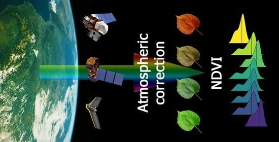
Effect of Atmospheric Corrections on NDVI: Intercomparability of Landsat 8, Sentinel-2, and UAV Sensors


Abstract
:
1. Introduction
2. Materials and Methods
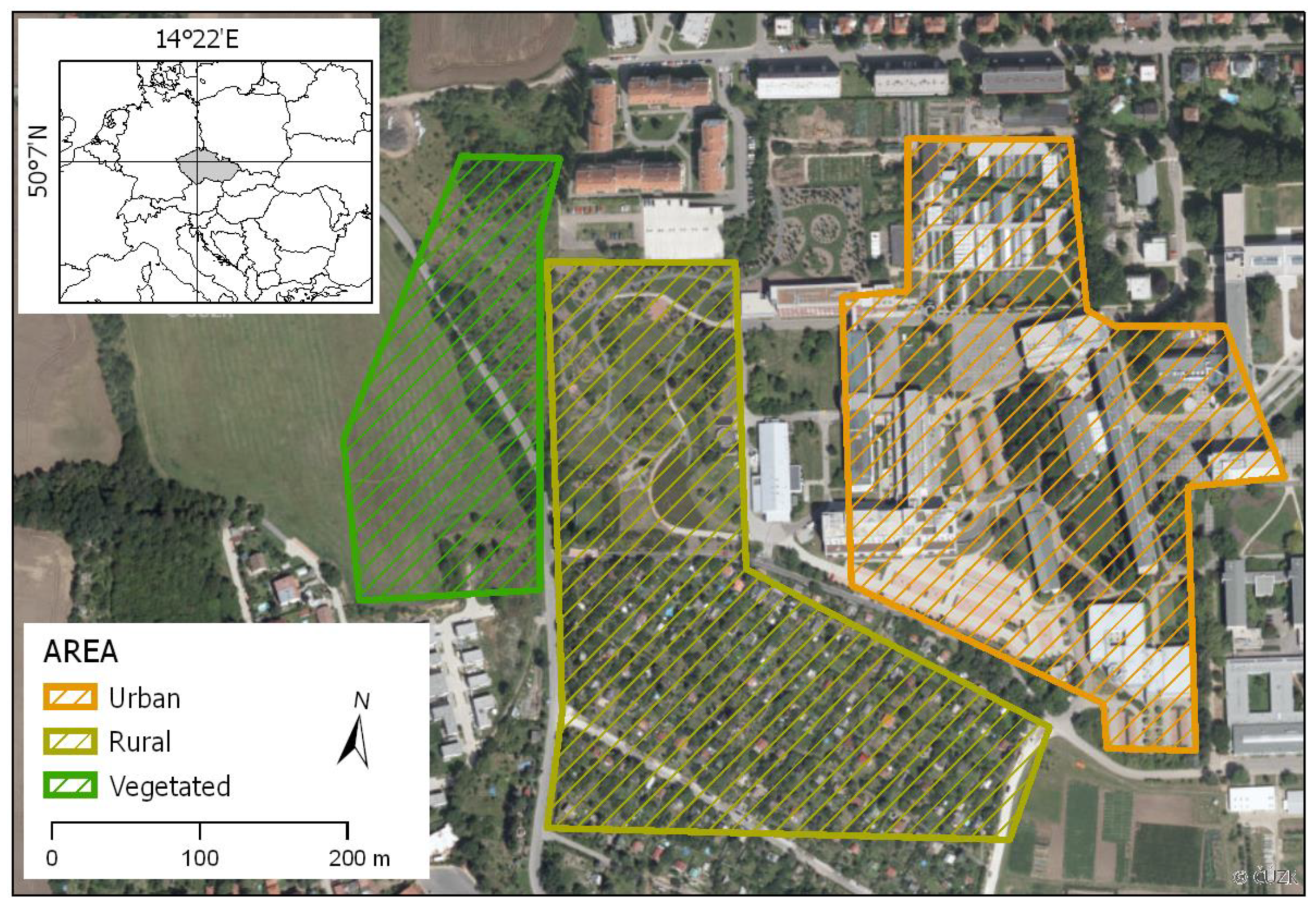
2.1. Study Site
2.2. Geospatial Imagery Data
2.2.1. Satellite Imagery Collection
2.2.2. UAV-Borne Data Acquisition and Processing
2.3. Atmospheric Correction Algorithms
2.3.1. Quick Atmospheric Correction (QUAC)
2.3.2. Dark Object Subtraction 1 (DOS)
2.3.3. Atmospheric Correction for OLI ‘lite’ (ACOLITE)
2.3.4. Fast Line-of-Sight Atmospheric Analysis of Hypercubes (FLAASH)
2.3.5. Second Simulation of Satellite Signal in the Solar Spectrum (6S)
2.3.6. Sen2Cor
2.4. Data Analysis
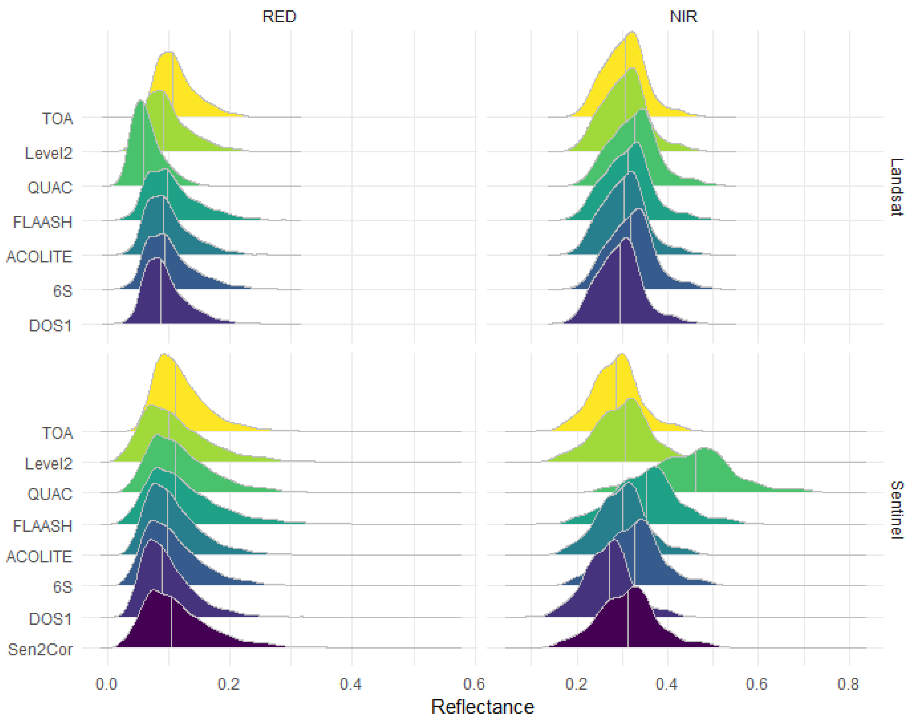
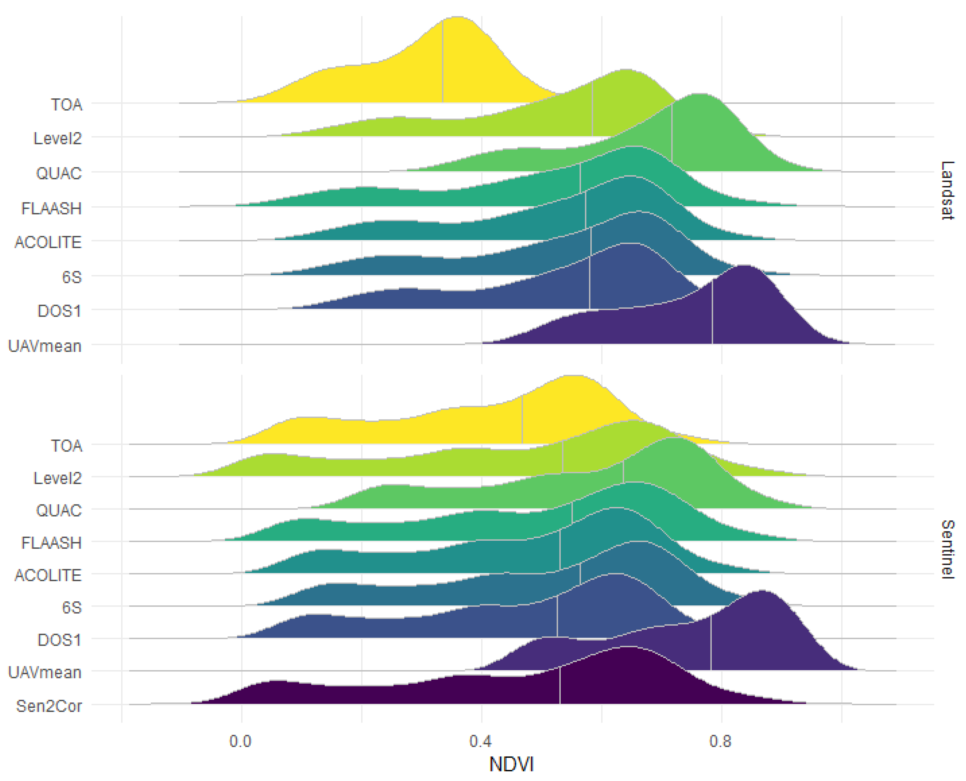
3. Results
4. Discussion
5. Conclusions
Author Contributions
Funding
Institutional Review Board Statement
Informed Consent Statement
Data Availability Statement
Conflicts of Interest
Appendix A

| Landsat 8 | UAV | TOA | DOS1 | 6S | ACOLITE | FLAASH | QUAC | Level2 | |
|---|---|---|---|---|---|---|---|---|---|
| UAV | 0.8878 | 0.8821 | 0.8901 | 0.8906 | 0.8909 | 0.8904 | 0.8882 | ||
| TOA | 0.8878 | 0.9807 | 0.9887 | 0.9903 | 0.9915 | 0.9889 | 0.9875 | ||
| DOS1 | 0.8821 | 0.9807 | 0.9963 | 0.9959 | 0.9955 | 0.9966 | 0.9959 | ||
| 6S | 0.8901 | 0.9887 | 0.9963 | 0.9999 | 0.9997 | 0.9998 | 0.9992 | ||
| ACOLITE | 0.8906 | 0.9903 | 0.9959 | 0.9999 | 0.9999 | 0.9998 | 0.9993 | ||
| FLAASH | 0.8909 | 0.9915 | 0.9955 | 0.9997 | 0.9999 | 0.9996 | 0.9993 | ||
| QUAC | 0.8904 | 0.9889 | 0.9966 | 0.9998 | 0.9998 | 0.9996 | 0.9989 | ||
| Level2 | 0.8882 | 0.9875 | 0.9959 | 0.9992 | 0.9993 | 0.9993 | 0.9989 | ||
| Sentinel-2 | UAV | TOA | DOS1 | 6S | ACOLITE | FLAASH | QUAC | Level2 | Sen2Cor |
| UAV | 0.8994 | 0.8991 | 0.8988 | 0.8993 | 0.8996 | 0.8988 | 0.8990 | 0.8993 | |
| TOA | 0.8994 | 0.9985 | 0.9982 | 0.9992 | 0.9995 | 0.9978 | 0.9982 | 0.9988 | |
| DOS1 | 0.8991 | 0.9985 | 0.9995 | 0.9995 | 0.9996 | 0.9996 | 0.9991 | 1.0000 | |
| 6S | 0.8988 | 0.9982 | 0.9995 | 0.9998 | 0.9996 | 0.9994 | 0.9996 | 0.9995 | |
| ACOLITE | 0.8993 | 0.9992 | 0.9995 | 0.9998 | 0.9999 | 0.9993 | 0.9995 | 0.9996 | |
| FLAASH | 0.8996 | 0.9995 | 0.9996 | 0.9996 | 0.9999 | 0.9991 | 0.9995 | 0.9997 | |
| QUAC | 0.8988 | 0.9978 | 0.9996 | 0.9994 | 0.9993 | 0.9991 | 0.9990 | 0.9996 | |
| Level2 | 0.8990 | 0.9982 | 0.9991 | 0.9996 | 0.9995 | 0.9995 | 0.9990 | 0.9992 | |
| Sen2Cor | 0.8993 | 0.9988 | 1.0000 | 0.9995 | 0.9996 | 0.9997 | 0.9996 | 0.9992 | |
Appendix B
| Landsat 8 | TOA | Level2 | QUAC | FLAASH | ACOLITE | 6S | |
|---|---|---|---|---|---|---|---|
| Level2 | <0.001 | ||||||
| QUAC | <0.001 | <0.001 | |||||
| FLAASH | <0.001 | 0.098 | <0.001 | ||||
| ACOLITE | <0.001 | 1.000 | <0.001 | <0.001 | |||
| 6S | <0.001 | 0.069 | <0.001 | <0.001 | <0.001 | ||
| DOS1 | <0.001 | 0.002 | <0.001 | <0.001 | <0.001 | 1.000 | |
| Sentinel-2 | TOA | Level2 | QUAC | FLAASH | ACOLITE | 6S | DOS1 |
| Level2 | <0.001 | ||||||
| QUAC | <0.001 | <0.001 | |||||
| FLAASH | <0.001 | <0.001 | <0.001 | ||||
| ACOLITE | <0.001 | 0.610 | <0.001 | <0.001 | |||
| 6S | <0.001 | <0.001 | <0.001 | <0.001 | <0.001 | ||
| DOS1 | <0.001 | 1.000 | <0.001 | <0.001 | <0.001 | <0.001 | |
| Sen2Cor | <0.001 | <0.001 | <0.001 | <0.001 | 0.010 | <0.001 | 1.000 |
References
- Rouse, J.W., Jr.; Haas, R.H.; Schell, J.A.; Deering, D.W. Monitoring the Vernal Advancement and Retrogradation (Green Wave Effect) of Natural Vegetation; Texas A & M University, Remote Sensing Center: College Station, TX, USA, 1973. [Google Scholar]
- Tucker, C.J. Red and photographic infrared linear combinations for monitoring vegetation. Remote Sens. Environ. 1979, 8, 127–150. [Google Scholar] [CrossRef] [Green Version]
- Nijland, W.; de Jong, R.; de Jong, S.M.; Wulder, M.A.; Bater, C.W.; Coops, N.C. Monitoring plant condition and phenology using infrared sensitive consumer grade digital cameras. Agric. For. Meteorol. 2014, 184, 98–106. [Google Scholar] [CrossRef] [Green Version]
- Pettorelli, N.; Ryan, S.; Mueller, T.; Bunnefeld, N.; Jedrzejewska, B.; Lima, M.; Kausrud, K. The Normalized Difference Vegetation Index (NDVI): Unforeseen successes in animal ecology. Clim. Res. 2011, 46, 15–27. [Google Scholar] [CrossRef]
- Sun, L.; Gao, F.; Anderson, M.C.; Kustas, W.P.; Alsina, M.M.; Sanchez, L.; Sams, B.; McKee, L.; Dulaney, W.; White, W.A.; et al. Daily mapping of 30 m LAI and NDVI for grape yield prediction in California vineyards. Remote Sens. 2017, 9, 317. [Google Scholar] [CrossRef] [Green Version]
- Ghaderpour, E.; Ben Abbes, A.; Rhif, M.; Pagiatakis, S.D.; Farah, I.R. Non-stationary and unequally spaced NDVI time series analyses by the LSWAVE software. Int. J. Remote Sens. 2020, 41, 2374–2390. [Google Scholar] [CrossRef]
- Hazaymeh, K.; Hassan, Q.K. Remote sensing of agricultural drought monitoring: A state of art review. Aims Environ. Sci. 2016, 3, 604–630. [Google Scholar] [CrossRef]
- Defries, R.S.; Townshend, J.R. Ndvi-Derived Land Cover Classifications At a Global Scale. Int. J. Remote Sens. 1994, 15, 3567–3586. [Google Scholar] [CrossRef]
- Lunetta, R.S.; Knight, J.F.; Ediriwickrema, J.; Lyon, J.G.; Worthy, L.D. Land-cover change detection using multi-temporal MODIS NDVI data. Remote Sens. Environ. 2006, 105, 142–154. [Google Scholar] [CrossRef]
- Gandhi, G.M.; Parthiban, S.; Thummalu, N.; Christy, A. Ndvi: Vegetation Change Detection Using Remote Sensing and Gis—A Case Study of Vellore District. Procedia Comput. Sci. 2015, 57, 1199–1210. [Google Scholar] [CrossRef] [Green Version]
- Min, C.K.; Muchtar, A.; Bahar, A.; Udin, W.S. Landslide Assessment Using Normalized Difference Vegetation Index (NDVI). J. Trop. Resour. Sustain. Sci. 2016, 4, 98–104. [Google Scholar]
- Agapiou, A.; Hadjimitsis, D.G.; Papoutsa, C.; Alexakis, D.D.; Papadavid, G. The Importance of accounting for atmospheric effects in the application of NDVI and interpretation of satellite imagery supporting archaeological research: The case studies of Palaepaphos and Nea Paphos sites in Cyprus. Remote Sens. 2011, 3, 2605–2629. [Google Scholar] [CrossRef] [Green Version]
- Löfgren, O.; Prentice, H.C.; Moeckel, T.; Schmid, B.C.; Hall, K. Landscape history confounds the ability of the NDVI to detect fine-scale variation in grassland communities. Methods Ecol. Evol. 2018, 9, 2009–2018. [Google Scholar] [CrossRef]
- Neinavaz, E.; Skidmore, A.K.; Darvishzadeh, R. Effects of prediction accuracy of the proportion of vegetation cover on land surface emissivity and temperature using the NDVI threshold method. Int. J. Appl. Earth Obs. Geoinf. 2020, 85, 101984. [Google Scholar] [CrossRef]
- Liu, L.; Zhang, Y. Urban heat island analysis using the landsat TM data and ASTER Data: A case study in Hong Kong. Remote Sens. 2011, 3, 1535–1552. [Google Scholar] [CrossRef] [Green Version]
- Ke, Y.; Im, J.; Lee, J.; Gong, H.; Ryu, Y. Characteristics of Landsat 8 OLI-derived NDVI by comparison with multiple satellite sensors and in-situ observations. Remote Sens. Environ. 2015, 164, 298–313. [Google Scholar] [CrossRef]
- Houborg, R.; McCabe, M.F. High-Resolution NDVI from planet’s constellation of earth observing nano-satellites: A new data source for precision agriculture. Remote Sens. 2016, 8, 768. [Google Scholar] [CrossRef] [Green Version]
- Loveland, T.R.; Irons, J.R. Landsat 8: The plans, the reality, and the legacy. Remote Sens. Environ. 2016, 185, 1–6. [Google Scholar] [CrossRef] [Green Version]
- Drusch, M.; Del Bello, U.; Carlier, S.; Colin, O.; Fernandez, V.; Gascon, F.; Hoersch, B.; Isola, C.; Laberinti, P.; Martimort, P.; et al. Sentinel-2: ESA’s Optical High-Resolution Mission for GMES Operational Services. Remote Sens. Environ. 2012, 120, 25–36. [Google Scholar] [CrossRef]
- Teillet, P.M. Image correction for radiometric effects in remote sensing. Int. J. Remote Sens. 1986, 7, 1637–1651. [Google Scholar] [CrossRef]
- Hagolle, O.; Huc, M.; Pascual, D.V.; Dedieu, G. A multi-temporal and multi-spectral method to estimate aerosol optical thickness over land, for the atmospheric correction of FormoSat-2, LandSat, VENμS and Sentinel-2 images. Remote Sens. 2015, 7, 2668–2691. [Google Scholar] [CrossRef] [Green Version]
- Nazeer, M.; Nichol, J.E.; Yung, Y.K. Evaluation of atmospheric correction models and Landsat surface reflectance product in an urban coastal environment. Int. J. Remote Sens. 2014, 35, 6271–6291. [Google Scholar] [CrossRef]
- Song, C.; Woodcock, C.E.; Seto, K.C.; Lenney, M.P.; Macomber, S.A. Classification and change detection using Landsat TM data: When and how to correct atmospheric effects? Remote Sens. Environ. 2001, 75, 230–244. [Google Scholar] [CrossRef]
- Doxani, G.; Vermote, E.; Roger, J.C.; Gascon, F.; Adriaensen, S.; Frantz, D.; Hagolle, O.; Hollstein, A.; Kirches, G.; Li, F.; et al. Atmospheric correction inter-comparison exercise. Remote Sens. 2018, 10, 352. [Google Scholar] [CrossRef] [Green Version]
- Chavez, P.S. An improved dark-object subtraction technique for atmospheric scattering correction of multispectral data. Remote Sens. Environ. 1988, 24, 459–479. [Google Scholar] [CrossRef]
- Padró, J.C.; Muñoz, F.J.; Ávila, L.Á.; Pesquer, L.; Pons, X. Radiometric correction of Landsat-8 and Sentinel-2A scenes using drone imagery in synergy with field spectroradiometry. Remote Sens. 2018, 10, 1687. [Google Scholar] [CrossRef] [Green Version]
- Pádua, L.; Vanko, J.; Hruška, J.; Adão, T.; Sousa, J.J.; Peres, E.; Morais, R. UAS, sensors, and data processing in agroforestry: A review towards practical applications. Int. J. Remote Sens. 2017, 38, 2349–2391. [Google Scholar] [CrossRef]
- Mahiny, A.S.; Turner, B.J. A comparison of four common atmospheric correction methods. Photogramm. Eng. Remote. Sens. 2007, 73, 361–368. [Google Scholar] [CrossRef]
- Hadjimitsis, D.G.; Papadavid, G.; Agapiou, A.; Themistocleous, K.; Hadjimitsis, M.G.; Retalis, A.; Michaelides, S.; Chrysoulakis, N.; Toulios, L.; Clayton, C.R.I. Atmospheric correction for satellite remotely sensed data intended for agricultural applications: Impact on vegetation indices. Nat. Hazards Earth Syst. Sci. 2010, 10, 89–95. [Google Scholar] [CrossRef] [Green Version]
- ESA. Sentinel-2 MSI User Guide. Available online: Sentinel.esa.int/web/sentinel/user-guides/document-library (accessed on 16 April 2020).
- NASA. Spectral Response of the Operational Land Imager In-Band, Band-Average Relative Spectral Response. Available online: Landsat.gsfc.nasa.gov/preliminary-spectral-response-of-the-operational-land-imager-in-band-band-average-relative-spectral-response/ (accessed on 16 April 2020).
- SenseFly. User Manual multiSPEC 4C Camera; SenseFly: Cheseaux-sur-Lausanne, Switzerland, 2014. [Google Scholar]
- Spectral Sciences Inc. MODTRAN Demo. Available online: Modtran.spectral.com (accessed on 16 April 2020).
- Komárek, J.; Klouček, T.; Prošek, J. The potential of Unmanned Aerial Systems: A tool towards precision classification of hard-to-distinguish vegetation types? Int. J. Appl. Earth Obs. Geoinf. 2018, 71, 9–19. [Google Scholar] [CrossRef]
- Bernstein, L.S. Quick atmospheric correction code: Algorithm description and recent upgrades. Opt. Eng. 2012, 51, 111719. [Google Scholar] [CrossRef]
- Harris Geospatial Solutions Inc. ENVI Exelis Visual Information Solutions; Harris Geospatial Solutions Inc.: Boulder, CO, USA, 2018. [Google Scholar]
- Moran, M.S.; Jackson, R.D.; Slater, P.N.; Teillet, P.M. Evaluation of simplified procedures for retrieval of land surface reflectance factors from satellite sensor output. Remote Sens. Environ. 1992, 41, 169–184. [Google Scholar] [CrossRef]
- Valdivieso-Ros, C.; Alonso-Sarria, F.; Gomariz-Castillo, F. Effect of different atmospheric correction algorithms on sentinel-2 imagery classification accuracy in a semiarid mediterranean area. Remote Sens. 2021, 13, 1770. [Google Scholar] [CrossRef]
- Vanhellemont, Q.; Ruddick, K. Acolite for Sentinel-2: Aquatic applications of MSI imagery. In Proceedings of the Living Planet Symposium, Prague, Czech Republic, 9–13 May 2016; ESA: Paris, France, 2016; Volume SP-740, pp. 1–8. [Google Scholar]
- Harris Geospatial Solutions Inc. FLAASH Background. Available online: https://www.l3harrisgeospatial.com/docs/backgroundflaash.html#Matthew (accessed on 11 February 2020).
- Matthew, M.W.; Adler-golden, S.M.; Berk, A.; Richtsmeier, S.C.; Levine, R.Y.; Bernstein, L.S.; Acharya, P.K.; Anderson, G.P.; Felde, G.W.; Hoke, M.P.; et al. Status of atmospheric correction using a modtran4-based algorithm. Int. Soc. Opt. Photonics 2000, 4049, 199–207. [Google Scholar]
- Felde, G.W.; Anderson, G.P.; Cooley, T.W.; Matthew, M.W.; Adler-Golden, S.M.; Berk, A.; Lee, J. Analysis of Hyperion Data with the FLAASH Atmospheric Correction Algorithm. Int. Geosci. Remote Sens. Symp. 2003, 1, 90–92. [Google Scholar]
- Vermote, E.F.; Tanré, D.; Deuzé, J.L.; Herman, M.; Morcrette, J.J. Second simulation of the satellite signal in the solar spectrum, 6s: An overview. IEEE Trans. Geosci. Remote Sens. 1997, 35, 675–686. [Google Scholar] [CrossRef] [Green Version]
- GRASS Development Team i.atcorr. Available online: https://grass.osgeo.org/grass78/manuals/i.atcorr.html (accessed on 14 June 2020).
- Main-Knorn, M.; Pflug, B.; Louis, J.; Debaecker, V.; Müller-Wilm, U.; Gascon, F. Sen2Cor for Sentinel-2 Sen2Cor for Sentinel-2; Image and Signal Processing for Remote Sensing XXIII; International Society for Optics and Photonics: Warsaw, Poland, 2017; Volume 10427. [Google Scholar]
- Mueller-Wilm, U.; Devignot, O.; Pessiot, L. Sen2Cor Configuration and User Manual; ESA: Paris, France, 2019. [Google Scholar]
- ESRI 2019. ArcGIS Desktop: Release 10; Environmental Systems Research Institute: Redlands, CA, USA, 2019. [Google Scholar]
- R Core Team R 2017. R: A Language and Environment for Statistical Computin; R Foundation for Statistical Computing: Vienna, Austria, 2017; Available online: https://www.R-project.org/ (accessed on 16 April 2020).
- Xie, Y.; Zhao, X.; Li, L.; Wang, H. Calculating NDVI for Landsat7-ETM data after atmospheric correction using 6S model: A case study in Zhangye city. In Proceedings of the 18th International Conference on Geoinformatics, Beijing, China, 18–20 June 2010; IEEE: Piscataway, NJ, USA, 2010; pp. 1–4. [Google Scholar]
- Gouveia, C.; Trigo, R.M.; DaCamara, C.C. Drought and vegetation stress monitoring in Portugal using satellite data. Nat. Hazards Earth Syst. Sci. 2009, 9, 185–195. [Google Scholar] [CrossRef] [Green Version]
- Messina, G.; Peña, J.M.; Vizzari, M.; Modica, G. A Comparison of UAV and Satellites Multispectral Imagery in Monitoring Onion Crop. An Application in the ‘Cipolla Rossa di Tropea’ (Italy). Remote Sens. 2020, 12, 3424. [Google Scholar] [CrossRef]
- Wang, Y.; Ryu, D.; Park, S.; Fuentes, S.; O’Connell, M. Upscaling UAV-borne high resolution vegetation index to satellite resolutions over a vineyard. In Proceedings of the 22nd International Congress on Modelling and Simulation (MODSIM2017), Hobart, Australia, 3–8 December 2017; pp. 978–984. [Google Scholar]
- Lukas, V.; Novák, J.; Neudert, L.; Svobodova, I.; Rodriguez-Moreno, F.; Edrees, M.; Kren, J. The combination of UAV survey and Landsat imagery for monitoring of crop vigor in precision agriculture. Int. Arch. Photogramm. Remote Sens. Spat. Inf. Sci. ISPRS Arch. 2016, 41, 953–957. [Google Scholar] [CrossRef] [Green Version]
- Kavvadias, A.; Psomiadis, E.; Chanioti, M.; Gala, E.; Michas, S. Precision agriculture—Comparison and evaluation of innovative very high resolution (UAV) and LandSat data. CEUR Workshop Proc. 2015, 1498, 376–386. [Google Scholar]
- Ryu, J.-H.; Na, S.-I.; Cho, J. Inter-Comparison of Normalized Difference Vegetation Index Measured from Different Footprint Sizes in Cropland. Remote Sens. 2020, 12, 2980. [Google Scholar] [CrossRef]
- Nadal, J.L.V.; Franch, B.; Roger, J.C.; Skakun, S.; Vermote, E.; Justice, C. Spectrally adjusted surface reflectance and its dependence with NDVI for passive optical sensors. In Proceedings of the IGARSS 2018—2018 IEEE International Geoscience and Remote Sensing Symposium, Valencia, Spain, 22–27 July 2018; pp. 6452–6455. [Google Scholar]


| Landsat 8 | Sentinel-2 | Difference | ||||
|---|---|---|---|---|---|---|
| Median | IQR | Median | IQR | Median | IQR | |
| TOA | 0.334 | 0.148 | 0.468 | 0.279 | −0.133 | −0.130 |
| Level2 | 0.584 | 0.216 | 0.534 | 0.363 | 0.049 | −0.147 |
| QUAC | 0.717 | 0.176 | 0.635 | 0.277 | 0.082 | −0.101 |
| FLAASH | 0.564 | 0.270 | 0.551 | 0.329 | 0.013 | −0.060 |
| ACOLITE | 0.573 | 0.236 | 0.530 | 0.296 | 0.043 | −0.060 |
| 6S | 0.583 | 0.246 | 0.563 | 0.303 | 0.019 | −0.057 |
| DOS1 | 0.579 | 0.224 | 0.525 | 0.302 | 0.055 | −0.078 |
| UAV | 0.784 | 0.193 | 0.782 | 0.229 | ||
| Sen2Cor | 0.529 | 0.355 | ||||
| DOS1 | 6S | ACOLITE | FLAASH | QUAC | Level2 | TOA | Ʃ | |
|---|---|---|---|---|---|---|---|---|
| Rural | 0.045 | 0.017 | 0.043 | 0.014 | 0.067 | 0.013 | −0.167 | 0.031 |
| Urban | 0.097 | 0.058 | 0.074 | 0.046 | 0.150 | 0.146 | −0.037 | 0.535 |
| Vegetated | 0.073 | 0.046 | 0.069 | 0.049 | 0.087 | 0.040 | −0.142 | 0.223 |
Publisher’s Note: MDPI stays neutral with regard to jurisdictional claims in published maps and institutional affiliations. |
© 2021 by the authors. Licensee MDPI, Basel, Switzerland. This article is an open access article distributed under the terms and conditions of the Creative Commons Attribution (CC BY) license (https://creativecommons.org/licenses/by/4.0/).
Share and Cite
Moravec, D.; Komárek, J.; López-Cuervo Medina, S.; Molina, I. Effect of Atmospheric Corrections on NDVI: Intercomparability of Landsat 8, Sentinel-2, and UAV Sensors. Remote Sens. 2021, 13, 3550. https://0-doi-org.brum.beds.ac.uk/10.3390/rs13183550
Moravec D, Komárek J, López-Cuervo Medina S, Molina I. Effect of Atmospheric Corrections on NDVI: Intercomparability of Landsat 8, Sentinel-2, and UAV Sensors. Remote Sensing. 2021; 13(18):3550. https://0-doi-org.brum.beds.ac.uk/10.3390/rs13183550
Chicago/Turabian StyleMoravec, David, Jan Komárek, Serafín López-Cuervo Medina, and Iñigo Molina. 2021. "Effect of Atmospheric Corrections on NDVI: Intercomparability of Landsat 8, Sentinel-2, and UAV Sensors" Remote Sensing 13, no. 18: 3550. https://0-doi-org.brum.beds.ac.uk/10.3390/rs13183550