Article

Prototyping a Generic Algorithm for Crop Parameter Retrieval across the Season Using Radiative Transfer Model Inversion and Sentinel-2 Satellite Observations

1
Gisat Ltd., Milady Horákové 57, 17000 Praha, Czech Republic
2
Department of Applied Geoinformatics and Cartography, Faculty of Science, Charles University, Albertov 6, 12843 Praha, Czech Republic
3
Global Change Research Institute, Czech Academy of Sciences, Bělidla 986/4a, 60300 Brno, Czech Republic
*
Author to whom correspondence should be addressed.
Remote Sens. 2021, 13(18), 3659; https://0-doi-org.brum.beds.ac.uk/10.3390/rs13183659
Submission received: 31 July 2021 / Revised: 30 August 2021 / Accepted: 3 September 2021 / Published: 13 September 2021
(This article belongs to the Collection Sentinel-2: Science and Applications)

Abstract

:
In this study, Sentinel-2 data were used for the retrieval of three key biophysical parameters of crops: leaf area index (LAI), leaf chlorophyll content (LCC), and leaf water content (LWC) for dominant crop types in the Czech Republic, including winter wheat (Triticum aestivum), spring barley (Hordeum vulgare), winter rapeseed (Brassica napus subsp. napus), alfalfa (Medicago sativa), sugar beet (Beta vulgaris), and corn (Zea mays subsp. Mays) in different stages of crop development. Artificial neural networks were applied in combination with an approach using look-up tables that is based on PROSAIL simulations to retrieve the biophysical properties tailored for each crop type. Crop-specific PROSAIL model optimization and validation were based upon a large dataset of in situ measurements collected in 2017 and 2018 in lowland of Central Bohemia region. For LCC and LAI, respectively, low relative root mean square error (rRMSE; 25%, 37%) was achieved. Additionally, a relatively strong correlation with in situ measurements (r = 0.80) was obtained for LAI. On the contrary, the results of the LWC parameter retrieval proved to be unsatisfactory. We have developed a generic tool for biophysical monitoring of agricultural crops based on the interpretation of Sentinel-2 satellite data by inversion of the radiation transfer model. The resulting crop condition maps can serve as precision agriculture inputs for selective fertilizer and irrigation application as well as for yield potential assessment.

Graphical Abstract

1. Introduction

Remote sensing is a valuable tool for objectively and nondestructively assessing the status of terrestrial vegetation [1]. A wide range of remote-sensing applications have been developed to monitor the status and development of agricultural crops [2]. This has revolutionized the agriculture sector by introducing the concepts of so-called precision farming. The availability of detailed spatial information relating to, for example, crop vigor, crop heterogeneity, nitrogen fertilization needs, or crop water deficiency have enabled more effective crop management on the level of individual parcels. This can bring benefits in such forms as substantially reduced costs, higher yields, and diminished environmental pressures (e.g., by avoiding overfertilization that leads to nitrogen leaching). A review on using remote sensing for precision farming can be found for example in [3].
There exist numerous crop parameters that can be retrieved either directly or indirectly from remote-sensing observations. Direct parameters include the canopy structural parameters such as canopy height [4], leaf biomass [5], leaf water [6], chlorophyll content [7], and indirect parameters, e.g., the nitrogen content [8]. Variation in these parameters leads to direct changes in remotely observed canopy signal, including reflectance [9], emissivity [10,11], or backscattering [12] coefficient. These can then be used to develop a regression model examining the relationship between a crop variable of interest and the remote-sensing observation [13]. This approach offers fast and simple retrieval of vegetation parameters and can establish important correlations, but its practical use is limited by several facts. Empirical models are generally site specific. On top of that, the relationship between vegetation reflectance and biophysical variables is influenced also by canopy structure (e.g., leaf orientation) and the developed model is thus also species specific. Since vegetation spectral properties change in time due in relation to plant phenology, the relation to plant biophysics changes also in time (and the model is thus time specific). All these issues significantly limit applicability of empirical approach for developing a generic tool for biophysical crop monitoring.
Alternatively, a physics-based approach can be applied using an inversion of a crop radiative transfer model (RTM) against remote-sensing observations [14]. The parametrization of a crop radiative transfer model and its inversion against remote-sensing observations is a demanding task that requires large amounts of input data for representative simulations of crop spectral behavior across a wide range of possible crop scenarios. When successful, a canopy radiative transfer model offers generic, large-scale retrieval of crop parameters for a wide range of observation conditions, crop types, and their development stages. Indirect parameters of crops do not influence the remotely observed signal directly. Rather, their retrieval typically requires synthesis of multisource data (e.g., remote-sensing observations, meteorological variables, in situ observations) in a land surface process model. In this way, numerous crop parameters, including, for example, crop yield [15] and gross primary production [16] can be predicted.
The high complexity and non-linearity of crop variables retrieval from the remote-sensing observation (regardless of whether empirically obtained or RTM simulated) requires usage of advanced regression methods [5]. Such powerful regression methods are non-linear machine learning techniques, e.g., support vector regression (SVR) or artificial neural network (ANN) [5], that have been successfully used in the crop variable retrieval context since the early 2000s [2]. The advantages of the ANN approach are the ability to predict multiple variables at the output, the general rapidity in performing predictions after training and the stability of results [5].
Retrieved direct and indirect parameters may be used directly within the precision farming concept as a map of traits of interest and their farm-level heterogeneity [17] for variable application of, for example, fertilizers [18], insecticides, seeds, or watering.
In this study, we apply a physics-based approach to retrieve several direct crop parameters for dominant crop types of the Czech Republic, including winter wheat (Triticum aestivum), spring barley (Hordeum vulgare), winter rapeseed (Brassica napus subsp. napus), alfalfa (Medicago sativa), sugar beet (Beta vulgaris), and corn (Zea mays subsp. mays). It uses PROSAIL, which couples a leaf optical properties model and a canopy radiative transfer model, together with a large in situ dataset collected during field campaigns and the ANN regression approach.
Main research objective of this study was to test the applicability of radiative transfer inversion approach to retrieve crops parameters for a wide range of conditions, e.g., different crop types and their growing stages to design a generic yet crop specific calibrated tool for biophysical monitoring further applicable in precision farming concept.

2. Materials and Methods

2.1. In Situ Data Collection and Processing

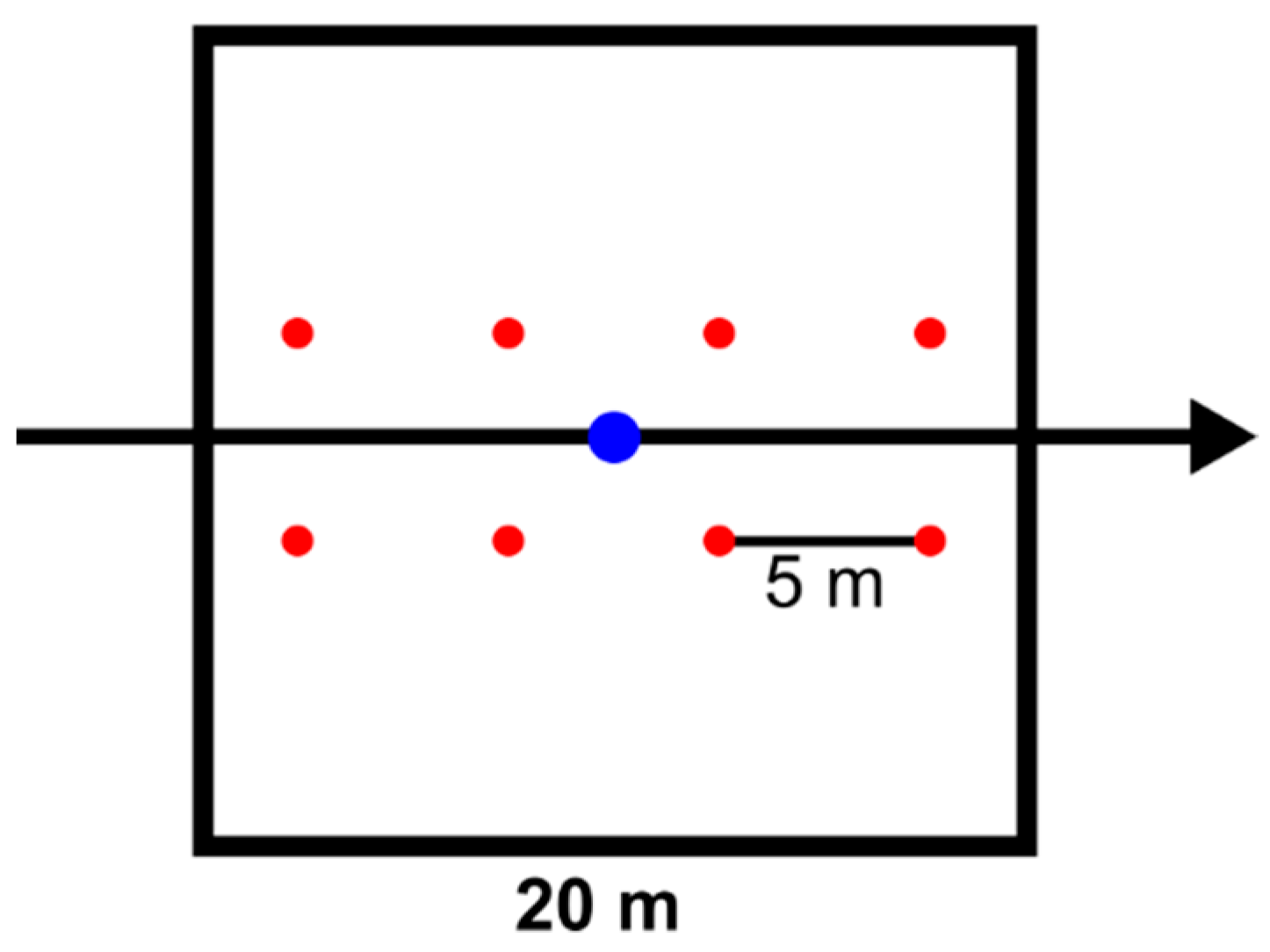
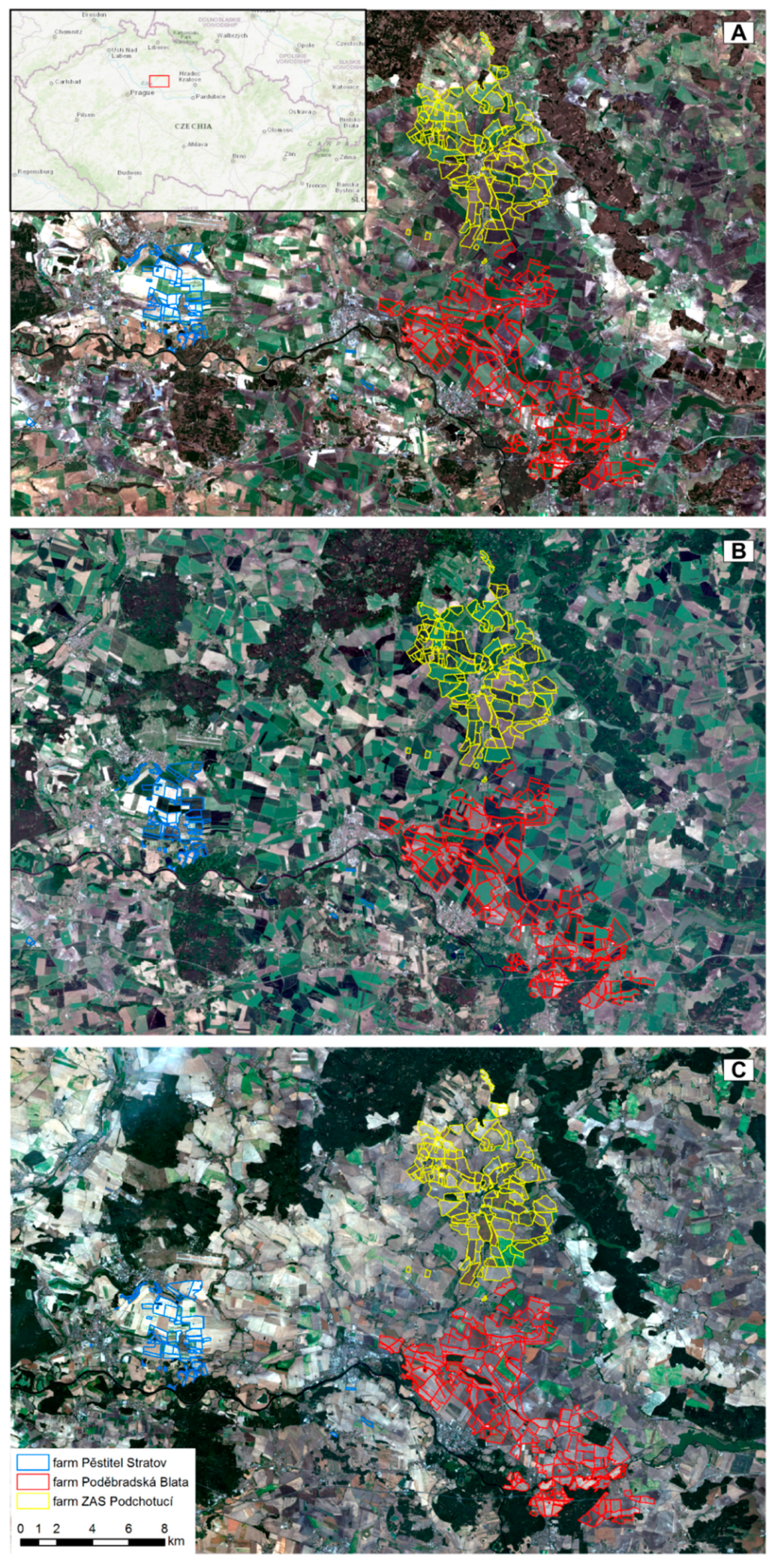
2.1.1. Test Sites and Sampling Design

Intensive ground sampling campaigns were organized during vegetation seasons in 2017 (3 campaigns) and 2018 (5 campaigns) to (1) collect reference data for assessing the atmospheric corrections of Sentinel-2 data, (2) perform representative parameterization of the PROSAIL radiative transfer model, and (3) obtain a reference database of in situ measurements for validation of crop biophysical parameter retrievals. Campaigns were conducted at selected agricultural parcels of cooperating farms namely: Poděbradská Blata (50.16° N, 15.16° E), Pěstitel Stratov (50.19° N, 14.91° E), and ZAS Podchotucí (50.28° N, 15.10° E). The overview map of those parcels is shown together with true color Sentinel-2 images for different parts of the growing season in Appendix A Figure A1. All of these farms are situated in lowland of Central Bohemia region known as Polabí (Elbeland). Thanks to favorable climatic conditions (mean annual temperature 8–9 °C, sum of temperature over 10 °C 2600–2800, mean annual precipitation 500–600 mm), it is one of the most fertile and productive areas in the Czech Republic. Representative dates had to be selected to accommodate differences in phenology while covering all growing states of the crops. Selection was based on the results of analyzing temporal profiles for normalized difference vegetation index (NDVI) [19] used to describe vegetation phenology. The timing of the campaigns in relation to the phenological development of crops is shown along with the number of sampled points in Figure 1. In total, the ground sampling activities were performed in the following extent:
  • Eighteen parcels (7 × winter wheat, 4 × spring barley, 5 × winter rapeseed, 1 × alfalfa, 1 × sugar beet, 1 × corn) including 188 reference points in 2017.
  • Twenty-one parcels (3 × winter wheat, 2 × spring barley, 6 × alfalfa, 4 × sugar beet, 4 × corn) including 244 reference points in 2018.
Even as the collected in situ measurements had to be representative, they also should cover sufficient variability within the variables of interest. Selection of the reference parcels was consulted with the agronomists working at the cooperating farms. A transect of at least five reference points with minimum spacing of 40 m (= 2 Sentinel-2 pixels) was established at each reference parcel in order to cover the maximum variability in crop condition. Location of the transect on each parcel was designed with the help of an NDVI map generated from the latest cloud-free Sentinel-2 or Landsat-8 scene prior to the planned ground campaign (Figure 2). The spatial setting of the particular transects takes into consideration (a) intra-field variability but also (b) representative coverage of both “high productivity” and “low productivity” areas in terms of whole farm. At each sampling point, multiple measurements were made and then averaged to reduce the risk of measurement error. Coordinates of reference points were measured using a Garmin Oregon 300 field GPS receiver with a declared spatial accuracy between 3–5 m [20].

2.1.2. Measurements of Crop Leaf Biochemical Traits

Leaf chlorophyll content was measured nondestructively using a handheld Force-A Dualex device [21]. The leaf chlorophyll content was estimated from leaf transmittance measurements of narrow wavelengths that strongly correlate with changes in chlorophyll content. Ten measurements were performed at each sampling point and the average of these measurements was calculated as the reference chlorophyll value for the given sampling point. The main benefit of using the Force-A Dualex device is linear response of its readings to the increasing chlorophyll content (in contrast with other widely used chlorophyll meters SPAD and CCM-200 exhibiting non-linear response) [22]. According to [22], the Dualex reading can be considered as equivalent to leaf chlorophyll content in µg/cm2. The Dualex calibration model (based on comparing device readings against chlorophyll extracts) shows globally R2 = 0.88 and absolute RMSE = 5.20 µg/cm2 or R2 = 0.96 and absolute RMSE = 6.36 µg/cm2 in case of wheat and corn samples [22].
Leaf water content was determined gravimetrically as the difference between leaf fresh (FW) and dry (DW) weights. Collected leaf samples were transported into a mobile laboratory immediately after being cut from the canopy. Here, fresh weight was measured using laboratory scales (with 0.001 g precision). A desktop scanner was then used to estimate samples’ projected leaf area (LAP). Finally, leaf samples were dried for at least 48 h in an electric dryer at 70 °C and then weighed again to obtain their dry weights. The leaf water content expressed as equivalent water thickness (EWT (cm)) was then calculated as EWT = (FW − DW)/LAP. In addition to the water content, specific leaf area (cm2/g) and leaf specific weight (g/cm2) were calculated.

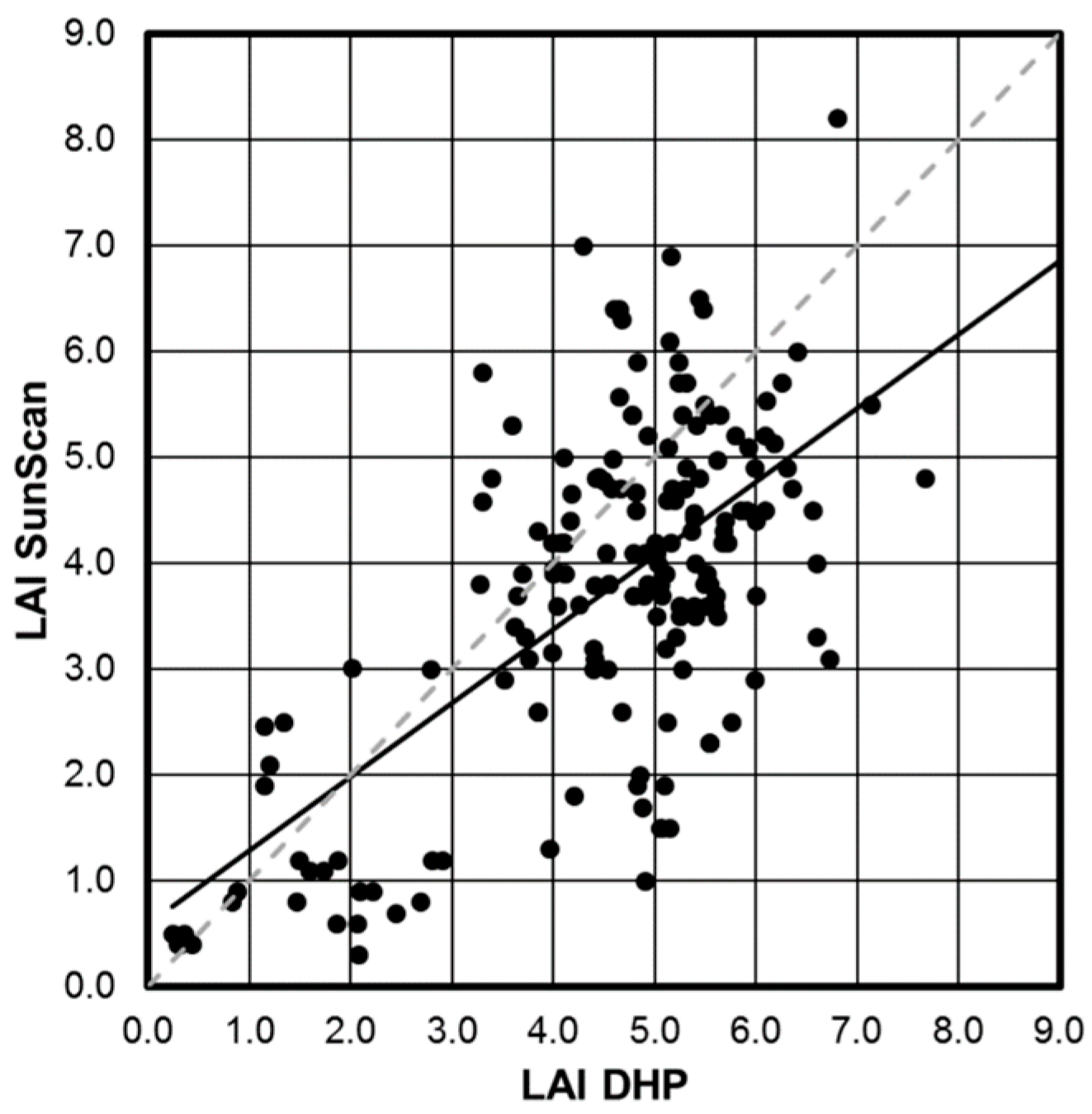
2.1.3. Measurements of Crop Structural Traits

Reference values of leaf area index (LAI) as a measure of crop leaf biomass and canopy closure were obtained by two different methods: (1) using a Delta-T SunScan device [23], and (2) from digital hemispherical photography (DHP). Two methods were used due to the applicability of each for different crop canopy conditions and development phases. In the case of the SunScan device, five measurements were collected at each sampling point and averaged into a single reference value. Similarly, eight DHP images were taken at each sampling spot using a Canon 700D digital camera equipped with a Sigma 4.5 mm f/2.8 circular fisheye lens. Sampling design covering an area of 20 × 20 m (corresponding to one Sentinel-2 pixel represented by the given sampling point) is shown in Figure 3. All images were taken using a tripod and horizontally levelled, resulting in sampling of the entire upper hemisphere with 180° circular field of view. Areas of the images that were obscured (e.g., by tripod) were masked manually. Next, the images were thresholded into binary masks of vegetation canopies. Sequences of the eight DHP images referring to one particular sampling point were then processed using the CanEye software [24], where LAI was inverted from angular distributions of canopy gaps. Both of the two inputs required by the CanEye software (optical center of the hemispherical images and projection function) were calibrated following instructions available in CanEye user manual and with help of the CanEye author [24].
Cases when both DHP-based and SunScan LAI measurements had been performed at the same time were used to check the relationships between the LAI values estimated by the two methods. A simple linear transformation of the SunScan-based LAI values was defined and applied to ensure maximal intercomparability of the two LAI datasets (see Figure 4 and Equation (3)).

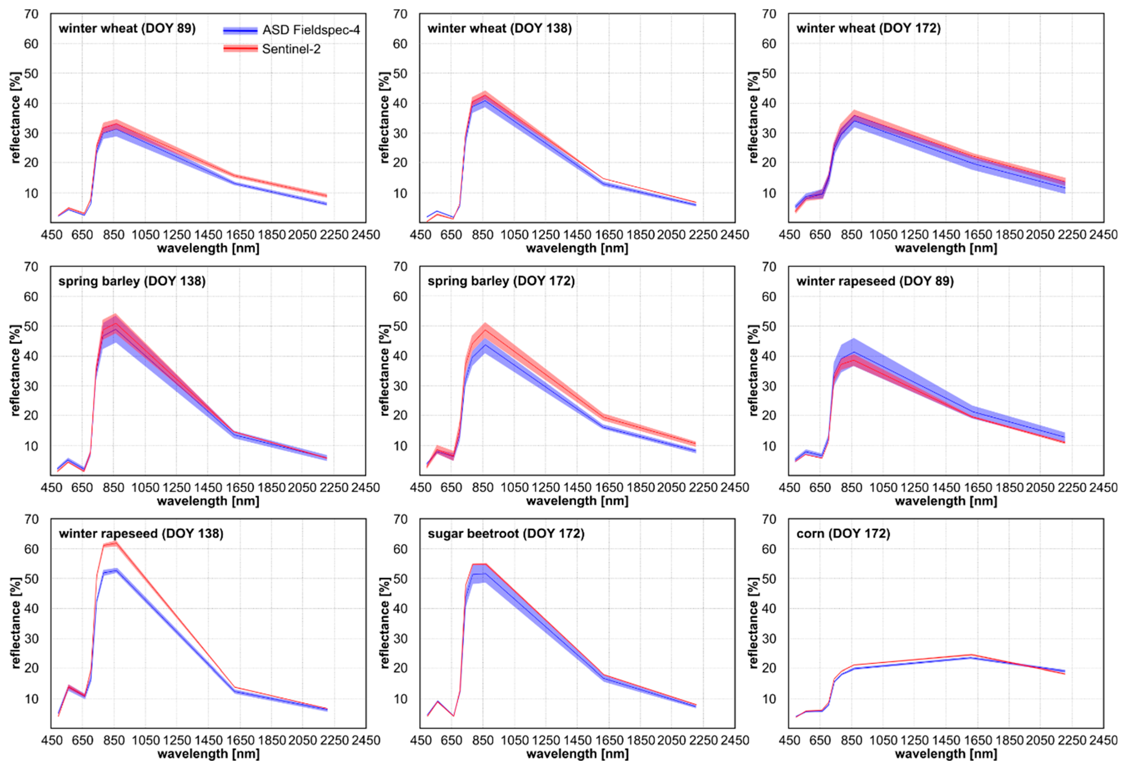
2.1.4. Measurements of Leaf and Canopy Spectra

Optical properties were measured using an ASD FieldSpec 4 field spectroradiometer [25]. The device measures incoming radiation in the spectral range from 350 to 2500 nm with 1 nm sampling interval. Different modes of operation allowed us to measure various remote-sensing quantities, ranging from surface (top-of-canopy) reflectance, leaf reflectance, and transmittance to incoming irradiance. We used the spectroradiometer to measure crops’ (1) top-of-canopy reflectance, and (2) leaf-level reflectance and transmittance.
The measurements followed a general sampling scheme, with several campaigns targeting phenological progress of the crops of interest. Top-of-canopy measurements were conducted using the ASD FieldSpec 4 with bare-fiber optics attached to the pistol grip. The measurements were performed under natural illumination conditions, which necessitated frequent collection of calibrated white reference (99% Spectralon surface reflectance panel with 12.7 cm square). After taking the reference measurement, we collected at each sampling point (the same for all sampled quantities, see Section 2.1.1) an average reflectance from four transects of a square with 10 m sides. These measurements were used to (a) validate the performance of atmospheric corrections of Sentinel-2 images, and (b) assess goodness of fit between the theoretical canopy radiative transfer modeling in the PROSAIL coupled model (see Section 3.2.1) and measured ground and satellite reflectances.
Leaf-level optical properties were measured using an attached ASD RTS-3ZC integrating sphere [25]. This allowed us to measure hemispherically integrated reflectance and transmittance of sampled leaves in a wide spectral range from 350 to 2500 nm with a 1 nm sampling interval. The measurements followed standard protocol as recommended by the manufacturer. The instrument was preheated for at least 20 min to avoid changes in radiometric characteristics. In total, 50 measurements were averaged for both white reference and the sample measurement. The leaf-level reflectance and transmittance measurements were used for (a) direct retrieval of the numbers N for the crops of interest (see Section 2.2.1 for details of PROSAIL model parametrization), and (b) collection of input reflectance for leaf optical properties.

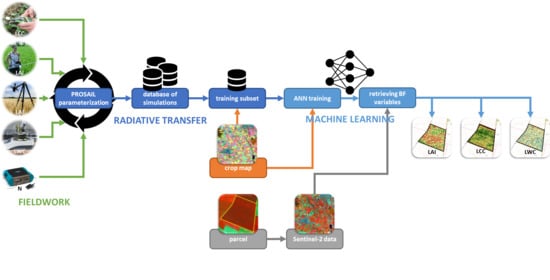
2.2. Radiative Transfer

2.2.1. PROSAIL Model Parametrization

In this study, the widely used PROSAIL radiative transfer model [26,27,28] was selected to simulate canopy spectral signatures of the studied crops in forward mode. The PROSAIL model combines the leaf-level PROSPECT and canopy-level SAIL models [29,30,31]. Specifically used was the Python implementation of the PROSPECT5 and 4-SAIL model version [32]. PROSAIL input parameters consist of leaf biochemical characteristics (e.g., chlorophyll and carotenoid content, water and dry matter content, brown pigment content), structural parameters of leaves (N) and canopy (LAI, LIDFa, LIDFb, Hspot), properties of illumination and observation geometry (solar zenith and azimuth angle, observation zenith and azimuth angle, fraction of diffuse incoming solar radiation), and the background soil spectra. The output of the PROSAIL model is simulated top-of-canopy spectral reflectance in wavelength range 400–2500 nm with 1 nm step.
A parametrization was performed in order to adjust the PROSAIL model for the six crops of interest. The aim was to determine the most suitable combination of input parameters that are not directly measurable in the field. We parameterized three PROSAIL input parameters: LIDFa, LIDFb, and Hspot. The parametrization’s principle consists in running the radiative transfer model iteratively for a specified range of the estimated parameters, whereas the rest of the input parameters (N, LCC, carotenoid content [Cx], LWC, dry specific leaf weight [SLW], and LAI) are fixed using field measurements (a strong linear correlation with LCC was found for parameter Cx [33]). The simulated canopy spectra are then compared with the reference spectra and the match is assessed by the root mean square error (RMSE). We used cloud-free Sentinel-2 (considering S2A in 2017 season and both S2A and S2B in 2018 season) images with the closest acquisition date as a reference. The simulated spectra were resampled to the Sentinel-2 spectral resolution using a sensor response function provided by the European Space Agency (the response functions for both variants, 2A and 2B, differ very little, so a single response function was used) [34]. Finally, the values of the calculated parameters were determined as weighted averages of parameters from 10 simulations with the best fit to the reference data (the weights were set as the reciprocals of the RMSE values). The statistical distribution functions were then designed for each crop and retrieved parameters (detailed in Section 3.2.1).
A particular case was the treatment of rapeseed during the flowering phase, because the flower reflectance considerably affects the overall canopy spectral signature. The PROSAIL model is not able to simulate the flowering rapeseed canopy. Our solution was to spectral mix the “green” and “yellow” components of the overall canopy biomass in a specific ratio, expressed by the following formula:
Rc = w · Rf + (1 − w) · Rg
where Rc corresponds to the whole canopy reflectance and Rf and Rg, respectively, represent reflectance of the flower and green biomass. The green biomass spectra (Rg) samples were extracted from Sentinel-2 images captured shortly before the flowering phase had begun, whereas the final (flowering) canopy reflectance (Rc) samples were taken from Sentinel-2 images of the same canopy in the middle of flowering phase. The rapeseed flowers spectra (Rf) were obtained by measuring the in situ flower samples with the portable ASD Fieldspec 4 spectroradiometer. The ratio of spectral mixing (w) was determined using a merit function assessing the fit between simulated and reference data. The proposed procedure was then applied to real Sentinel-2 data of the rapeseed canopy in flowering phase. The whole procedure of estimating the spectral mixing ratio (w) was performed on an empirical basis, meaning certain limitations in terms of site specificity. The value of Rg will be influenced by density and closure of the rapeseed canopy before starting of flowering phase. Similarly, the Rc will be influenced by intensity of rapeseed flowering (density of flowers) which may vary with different climatic/growing conditions (moreover, we assume that amount of green biomass does not change significantly from starting of the flowering phase). Although the procedure was developed using data obtained from rapeseed canopies with different density, it would be good to have data covering wider range of growing conditions to ensure greater robustness.

2.2.2. Design and Creation of Look-Up Tables

The biophysical parameters retrieval is based on a look-up table (LUT) approach. This method was chosen for its robustness and ease of use [14,28]. The crop-optimized PROSAIL model (see Section 2.2.1 for details) was run in forward mode. The canopy reflectances obtained were then resampled to Sentinel-2′s spectral resolution using the sensor spectral response function [34].
The simulated reflectances must cover any possible illumination conditions during the entire vegetation season in the Czech Republic so that the methodology is actually applicable in agricultural practice. The annual range of illumination geometry properties (sun zenith [SZ], sun azimuth [SA]) was determined based on Sentinel-2 time series (related to the time of a satellite’s passing over the Czech Republic) from 25° to 70° and from 150° to 170° for SZ and SA, respectively. The range of illumination geometry was divided in the interval of 5 ° into a total of 50 SZ–SA combinations.
For each of these 50 combinations, a set of 11,000 simulations (based on unique combinations of PROSAIL input parameters) was generated as a prediction model training subset (such a training subset size is considered as sufficient with respect to narrowly limited illumination conditions, while reasonable computational requirements for effective deployment in operational service). Soil background was approximated by generation spectra for various soil moisture levels using spectral mixing of dry- and wet-soil spectra given together with the PROSAIL model [32]. Three biophysical parameters of interest (LAI, LCC, LWC) were sampled randomly with uniform statistical distribution to cover all valid ranges of values. The ranges of LAI, LCC, and LWC were set according to previous studies [26] and values observed during our field campaigns as follow: 0–10 m2/m2 for LAI, 0–80 μg/cm2 for LCC, and 0.0005–0.07 cm for LWC (Table 1). The rest of the PROSAIL input parameters were either generated based on empirical distribution functions, determined by the parametrization procedure (LIDFa, LIDFb, and Hspot (see Section 2.2.1)) or based on the field data (Cm). The specific values are listed in Table 2. The value for Skyl (i.e., the ratio of diffuse versus total incident radiation) was set to 0.2, corresponding to cloudless sky [35].

2.3. Crop Biophysical Parameters Retrieval

2.3.1. Image Processing

The pair of Sentinel-2 satellites provides high spatial resolution (10, 20, and 60 m) imagery in 13 spectral bands covering visible, near-infrared, and short-wave infrared domains with high revisit time of 5 days (when both satellites are considered). In this study, the spectral bands with native spatial resolution of 10 and 20 m were considered (all in their 20 m version available in the L2A product). Atmospherically corrected top-of-canopy reflectance data (i.e., Level-2A) covering the entirety of the Czech Republic were generated for the years 2016, 2017, 2018, and 2019 (through 30 September 2019) using the SEN2COR processor that had been set up in accordance with the metadata for the processed scene [36].
Masks of the valid pixels were generated from the scene classification layer (SCL) created during the atmospheric correction using the SEN2COR tool. All pixels classified as follows were considered as invalid and thus excluded from further processing: 0 = no data, 1 = saturated or defective pixels, 3 = cloud shadows, 8 = medium probability clouds, 9 = high probability clouds, 10 = thin cirrus, and 11 = snow.
Because quality of atmospheric correction is one of the crucial factors influencing accuracy of the estimated crop biophysical variables, it must be checked prior to applying the crop biophysics retrieval algorithm to ensure that the canopy spectral signatures extracted from Sentinel-2 imagery are in agreement with the signatures measured in situ (see Section 2.1.4). Sentinel-2 top-of-canopy reflectances corresponding to reference points measured in situ were extracted for selected scenes acquired as close as possible to the times of the in situ campaigns (Table 3 lists reference Sentinel-2 scenes). These satellite canopy reflectances were then compared to the canopy-level spectra measured in situ (using ASD Fieldspec) and resampled from the original 1 nm resolution to the spectral characteristics of the Sentinel-2 MSI sensor using a sensor-specific response function [34]. The spectral signature of a pixel corresponding to a given reference point was compared to the average spectral reflectance measured in a transect corresponding to Sentinel-2 pixel size of 20 × 20 m. The RMSE between canopy reflectance (considering each Sentinel-2 band) and the spectra measured by ASD Fieldspec was calculated as:
RMSE = sqrt(sum (RSENb − RASDb)2/n),
where: RSENb is reflectance at the spectral band “b” extracted from Sentinel-2 data, RASDb is reflectance at the spectral band “b” extracted from data measured by ASD Fieldspec (after applying sensor-specific SRF), and n is the number of samples.

2.3.2. Biophysical Parameters Retrieval Approach

The artificial neural network (ANN) approach was chosen as a regression model for the retrieval of LAI, LCC, and LWC. A major advantage of ANNs lies in their computing power and ability to approximate any nonlinear relationship between different variables [37]. The ANN training phase was conducted using an LUT subset of 11,000 records. The training data was selected from the LUT database so that the illumination angles were as close as possible to the actual illumination angles of the Sentinel-2 scene (available in the scene metadata file). The training data were normalized and scaled to range 0–1 to ensure their equal influence in the model.
A one-hidden-layer, feed-forward, back-propagation neural network was implemented using the Python programming language and the TensorFlow machine learning library. We decided to use a relatively large hidden layer (50 neurons with widely used ReLu activation function) to cover the complex relationships between the biophysical characteristics of crops and its spectral properties. However, such a relatively large neural network requires an early stopping mechanism to prevent overfitting [38]. The training dataset was split into calibration (80%) and validation (20%) subset. Loss function (mean squared error) was monitored within the early stopping mechanism to stop the training process after reaching the baseline of 0.1 in validation loss and if there was no improvement in the next five epochs. The maximum number of epochs was set to 100, but this was never reached during the testing.
Two neural networks were designed: one for LAI retrieval, the other for LCC and LWC retrieval. The neural network for LCC and LWC retrieval uses all Sentinel-2 VIS to SWIR spectral bands with a native resolution of 10 m and 20 m, excluding the blue spectral band (B02), which is most sensitive to the quality of atmospheric correction. Green, red and red-edge spectral bands were excluded from LAI retrieval in order to reduce the adverse effect of the chlorophyll content on the LAI estimation (as these spectral bands are strongly affected by the chlorophyll content).
Estimated values of biophysical parameters are written into raster layers. Finally, the lowest and the highest possible values were set for each biophysical layer to avoid unrealistic values and while using the same rules as those for LUT generation (described in Section 2.2.2). However, situations where the estimated values fell out of the bounds region were very rare (0.73%, 0.12% and 1.39% of cases for LCC, LWC and LAI, respectively).

3. Results

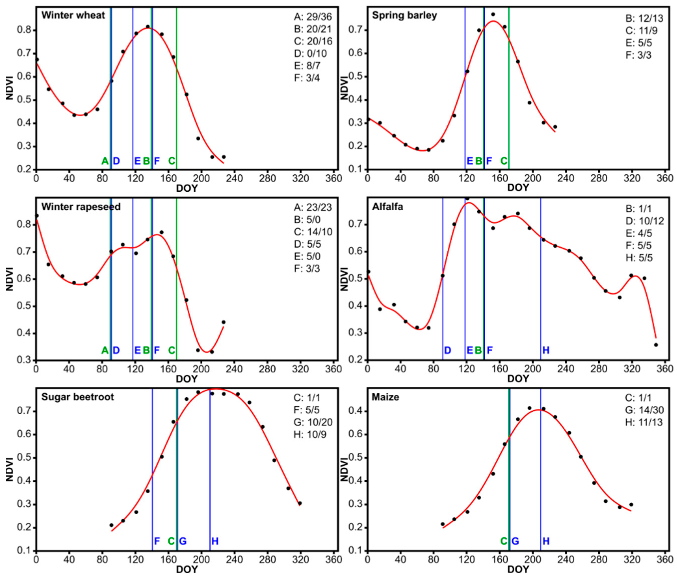
3.1. In Situ Crop Biochemical, Structural and Spectral Properties

3.1.1. In Situ Data Collection

The basic descriptive statistics of the in situ data collection for each crop of interest are documented in Table 4 (detailed statistics for both the calibration and validation data subsets are given in Table A1).
According to the practical experiences obtained during fieldworks, each of the used LAI measurement approaches seems to be more suitable for different type of vegetation canopies. Using the SunScan device seems to be more adequate for dense canopies, whereas its readings seem to be underestimated in case of sparse canopies and thus it can be recommended mostly for mature canopies. Just the opposite situation was observed in case of digital hemispherical photography which seems to be working well in case of young and sparse canopies, but uncertainty of LAI estimation increases with growing canopy density. A simple linear transformation was applied in order to harmonize SunScan-based and DHP-based LAI measurements as both types of measurement were taken at most of the sampling points (see Figure 4). This linear transformation is given by the following equation:
LAIt = 0.77 LAISS + 1.54
where LAIt is the transformed LAI estimation and LAISS is the SunScan measured LAI value.
The linear models shows R2 = 0.62 but we still consider it as a meaningful tool for establishing a generic database for validation of the LAI product across crop species with different canopy structure.
Transformed SunScan LAI values were merged with the DHP-based LAI estimations to produce a harmonized dataset of in situ LAI measurements for validating the Sentinel-2 based LAI product (see Section 3.3).
Leaf-level reflectance and transmittance measured by the ASD Fieldspec 4 spectroradiometer attached to the RTS-3ZC integrating sphere were used to estimate the optimal value of the PROSAIL’s structural parameter (N) for each crop. The number N represents leaf optical thickness and thus determines the ratio of the leaf reflectance and transmittance in PROSPECT leaf level simulations. The greater the leaf optical thickness (represented by a higher number N) the higher the reflectance-to-transmittance (R:T) ratio and vice versa. In the first step, PROSPECT was run iteratively with varying N value. The R:T ratios of the PROSPECT simulations at 1000 nm were further compared with the R:T ratios calculated from the leaf spectra measured in situ to find the most appropriate N value. Note that reflectance/transmittance in NIR domain has been taken into account because it is strongly correlated with the leaf internal structure and, at the same time, it is not influenced by, for example, the contents of leaf pigments, water, or other traits. The following numbers N ultimately were obtained for the crops of interest: winter wheat 1.44 ± 0.10, spring barley 1.57 ± 0.03, winter rapeseed 1.78 ± 0.27, alfalfa 1.53 ± 0.12, sugar beet 1.67 ± 0.19, and corn 1.28 ± 0.09.

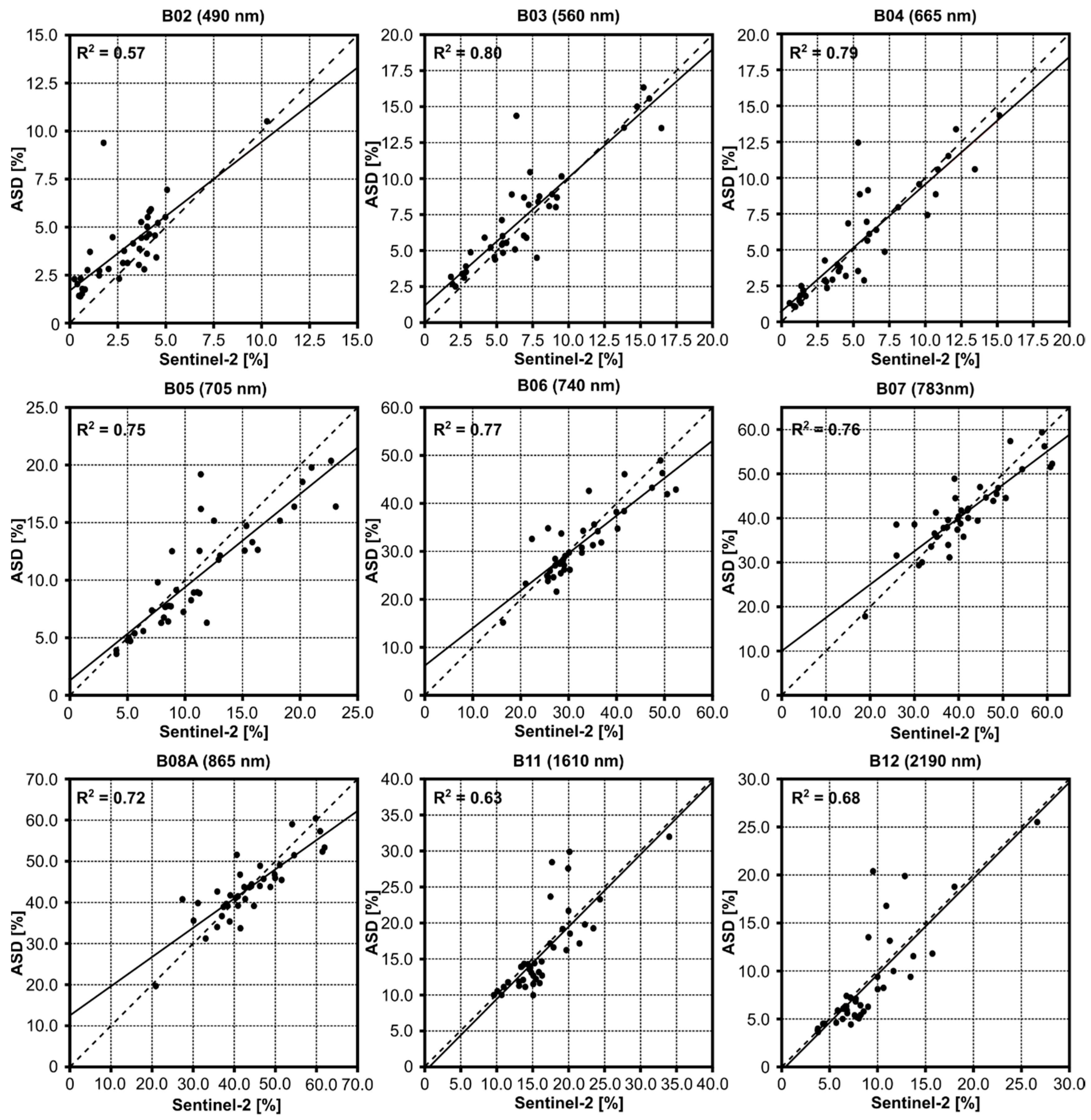
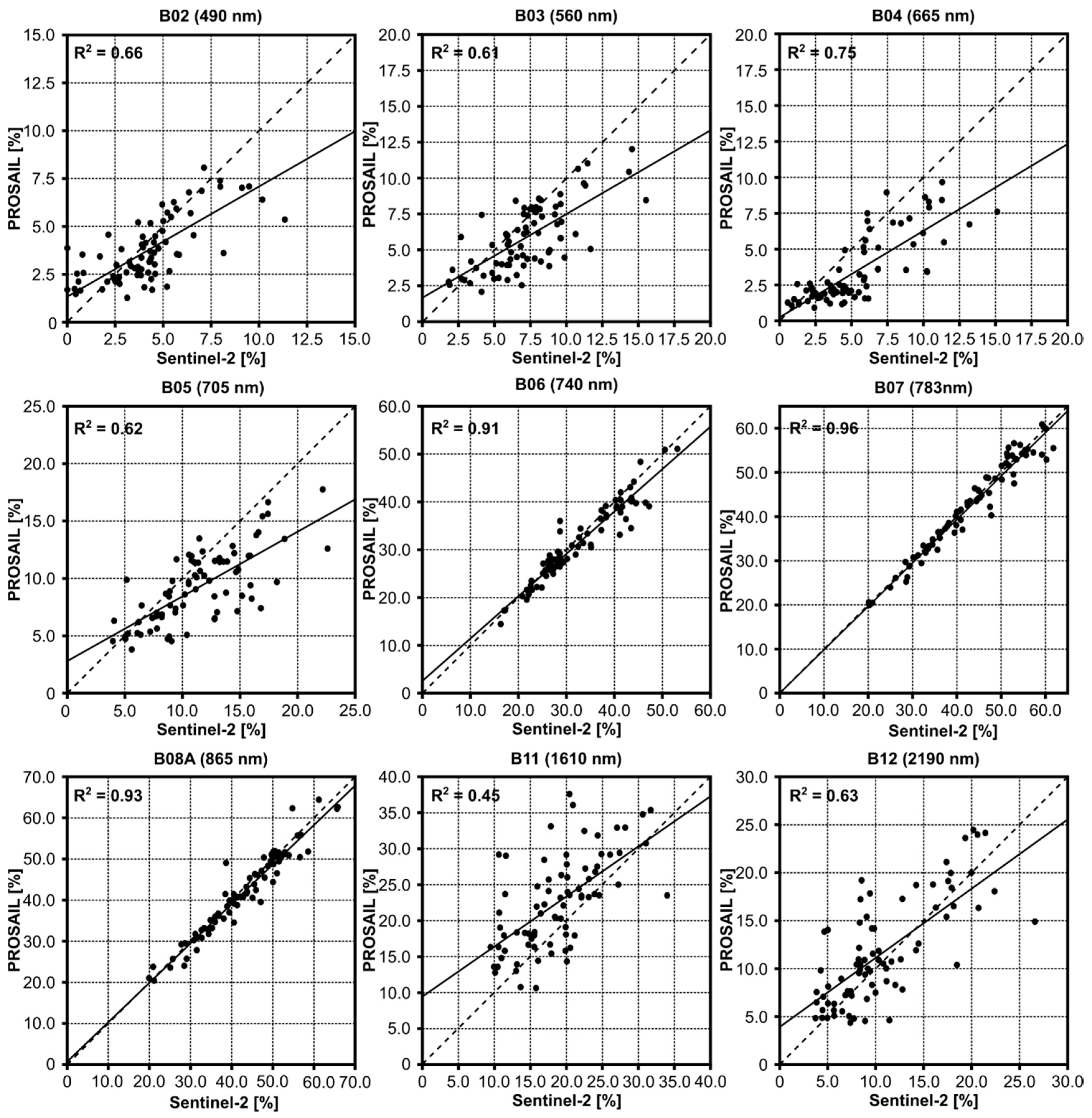
3.1.2. Quality of Sentinel-2 Atmospheric Correction

Sentinel-2 canopy reflectances were compared to the canopy-level spectra measured in situ to assess atmospheric quality correction (see Section 2.3.1 for details). For the vast majority of bands used, we have achieved a strong relationship (R2 > 0.7) over all crops of interest. The relationship achieved with the other three bands was R2 = 0.57, 0.63 and 0.68 for B02 (490 nm), B11 (1610 nm) and B12 (2190 nm), respectively, and can also be considered significant. The average rRMSE over all spectral bands and crops of interest was up to 30%. This demonstrates the good quality of the atmospheric corrections of Sentinel-2 data and direct comparability of crop in situ measurements with the satellite observations. Figure 5 shows scatter plots comparing Sentinel-2 and in situ measured canopy spectra across all Sentinel-2 spectral bands used. Examples of Sentinel-2 and in-situ measured spectra for the different development stages of crops of interest are shown in Figure A2.

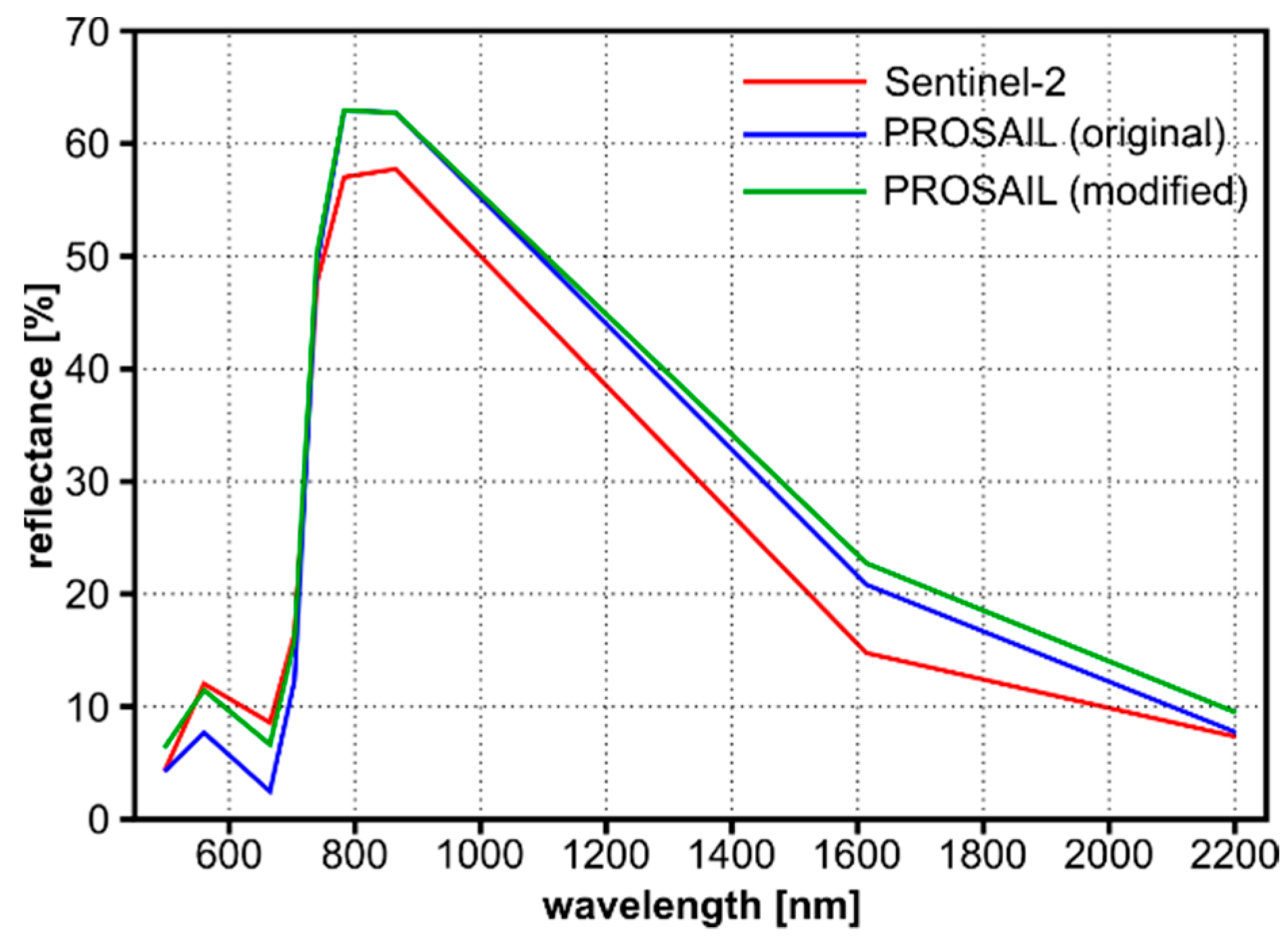
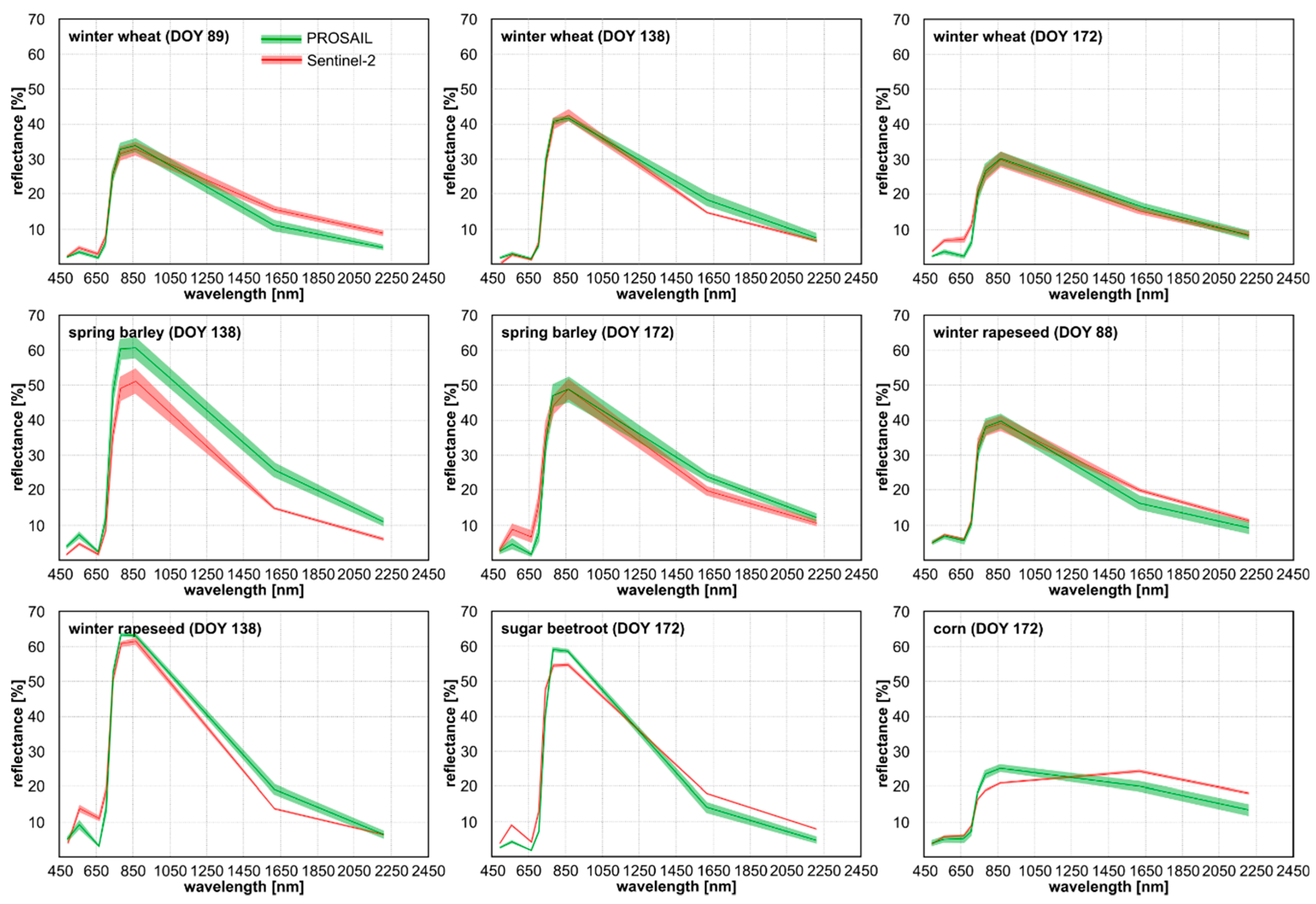
3.2. Modeling Crop-Specific Reflectance in the Radiative Transfer Model

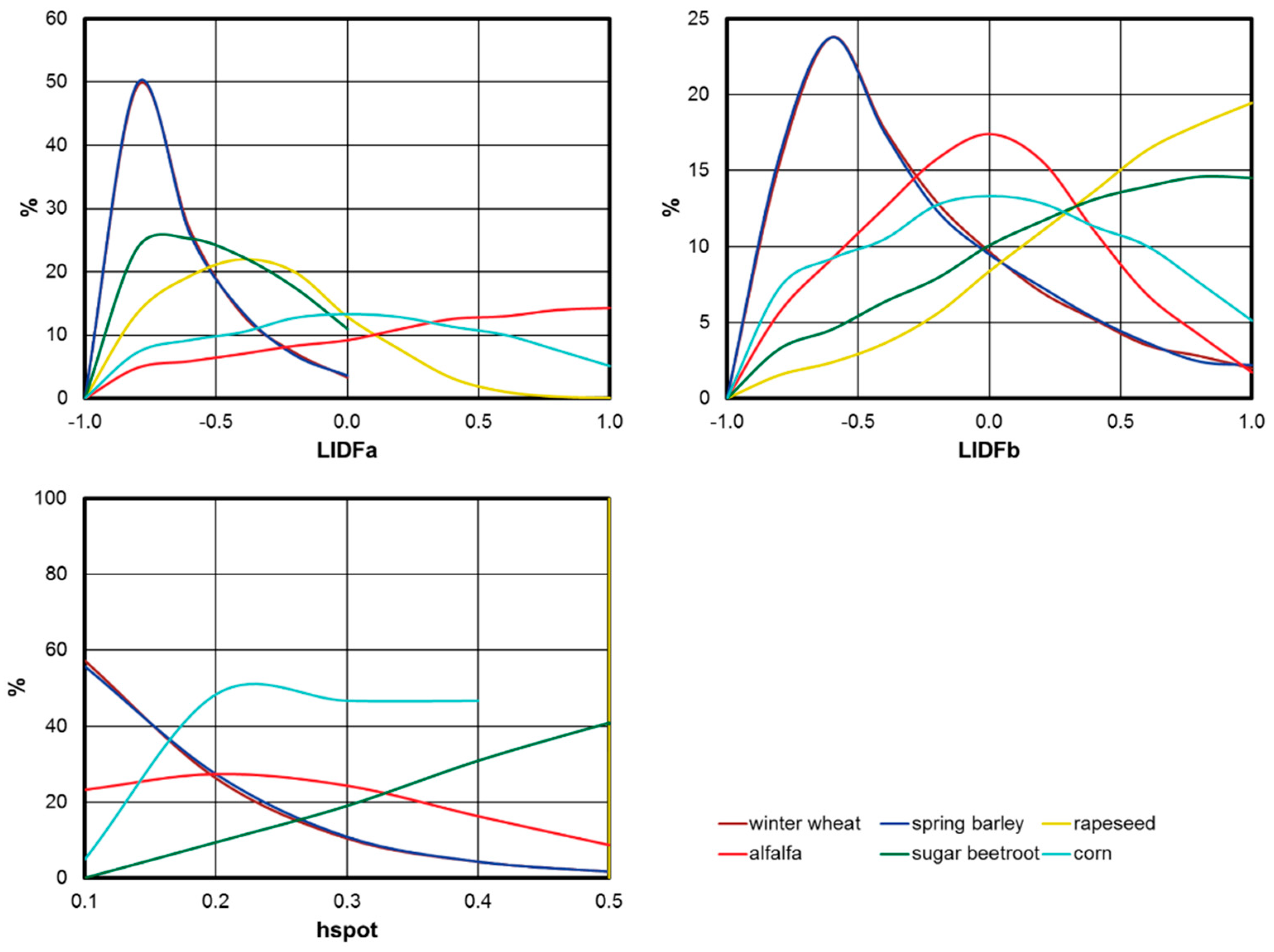
3.2.1. Crop-Specific Parametrization of the PROSAIL Radiative Transfer Model

Six crop-specific scenarios of PROSAIL parametrization were designed. For each crop of interest, an empirical distribution function of crop-specific structural PROSAIL model inputs (LIDFa, LIDFb, and Hspot) was constructed based on the frequency of their values obtained during the parameterization process. The main objective was to provide a generic yet representative statistical distribution of simulated parameters. Figure 6 shows the empirical distribution functions of LIDFa, LIDFb, and Hspot for six crops of interest extracted from LUTs.
A particular issue in radiative transfer model parametrization was to deal with any unrealistic PROSAIL input combinations, as these could lead to ambiguity in the model inversion. During leaf senescence, chlorophyll and water contents naturally decrease [39]. Acute water stress, however, has no immediate impact on leaf chlorophyll content [40]. Although there is no clear relationship between leaf chlorophyll and water content throughout the vegetation season, certain combinations of these parameters are indeed unrealistic (e.g., very low chlorophyll and high water content). The LCC–LWC relationships observed in situ (Figure 7) show that high chlorophyll concentrations are associated with a wide range (from low to high) of water contents but that low chlorophyll concentrations occur only with low water content. We therefore have introduced arbitrary water content limits (LWCmax) for three considered chlorophyll content levels (Figure 7):
1.  LCC < 20 μg/cm2: LWCmax = 0.02 cm
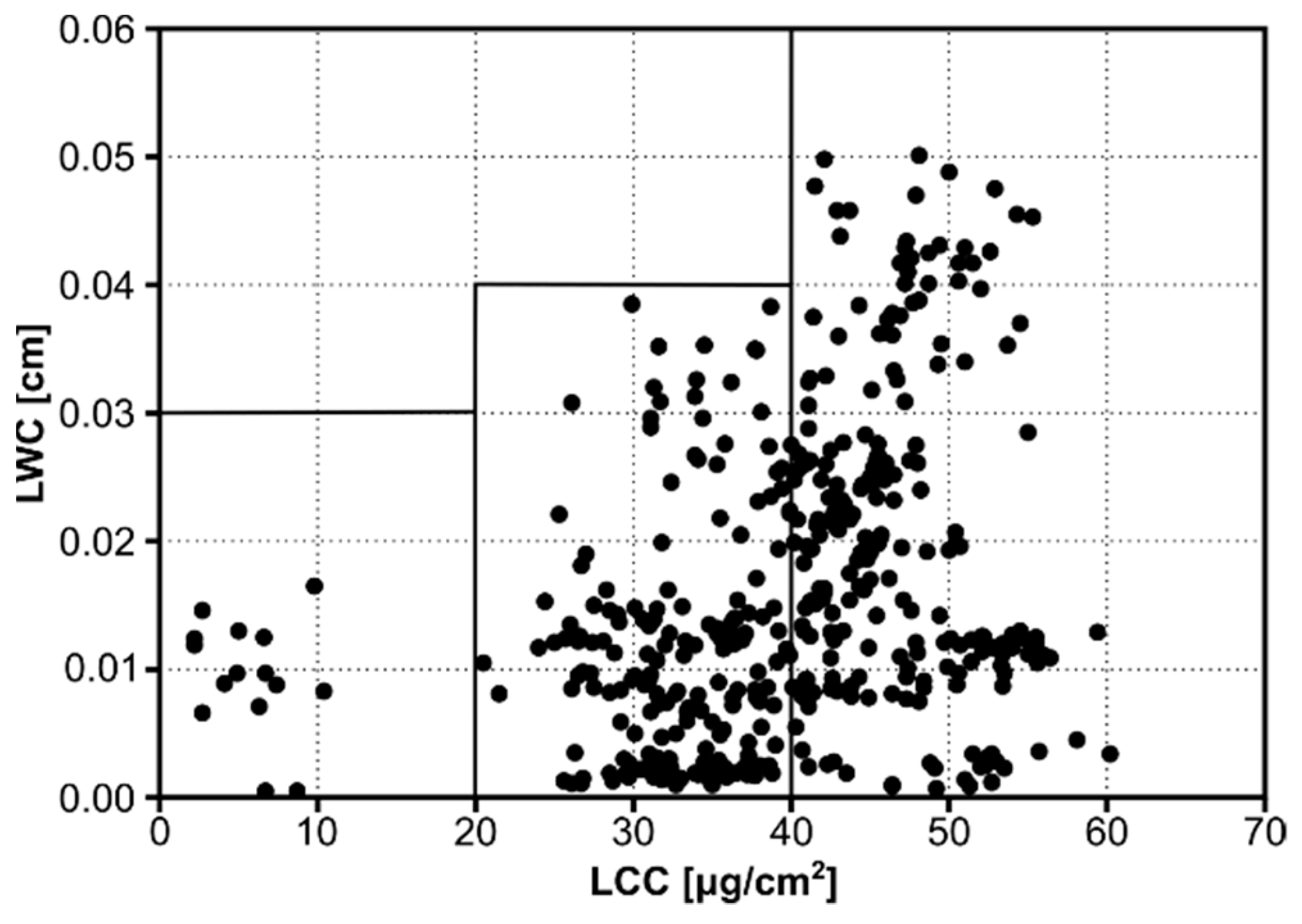
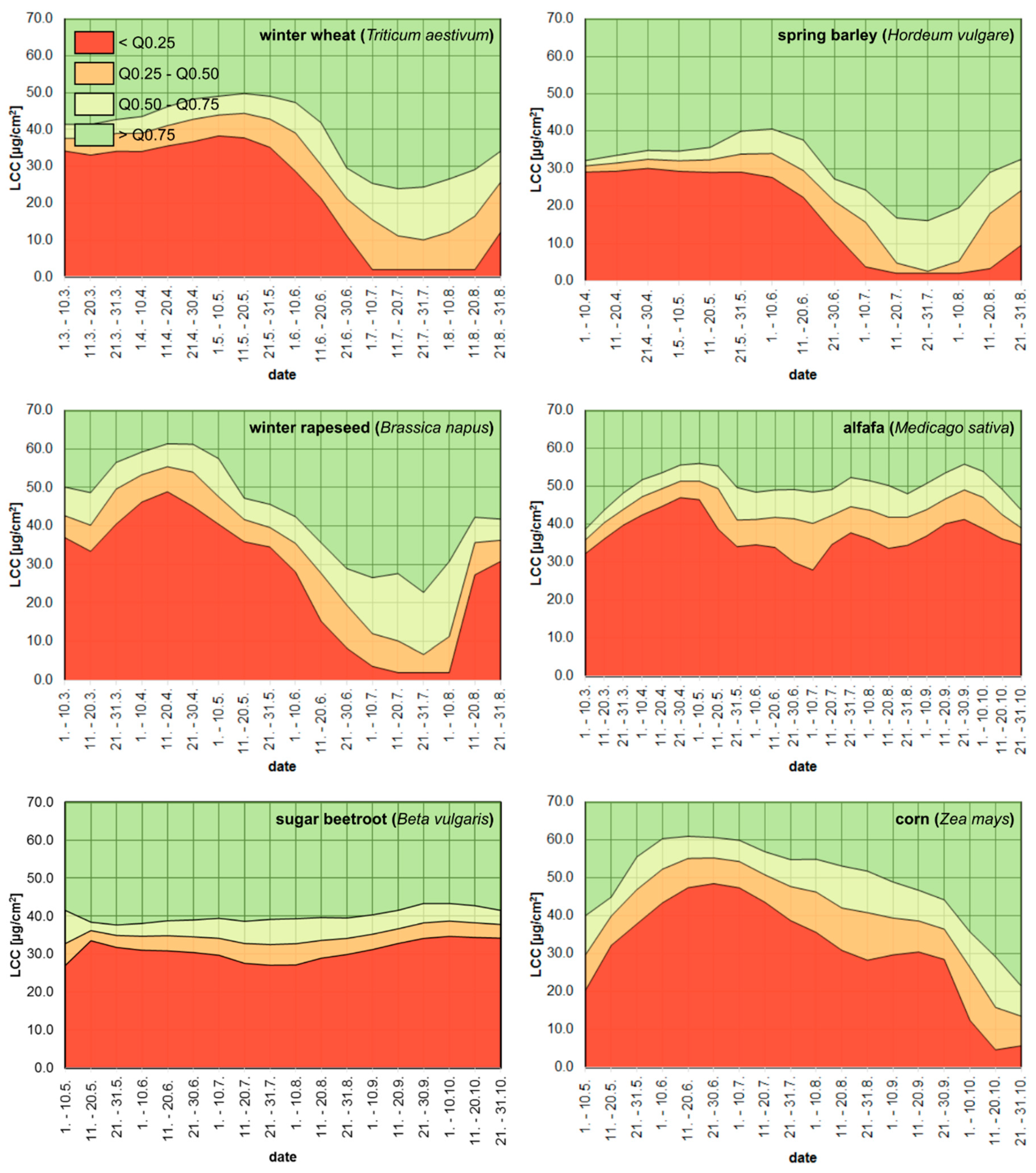
2.  20 μg/cm2 ≤ LCC < 40 μg/cm2: LWCmax = 0.04 cm
3.  LCC >= 40 μg/cm2: LWCmax = 0.07 cm
Synthetic spectral signature of flowering rapeseed is obtained by spectral mixing of the “green” and “yellow” components of the overall canopy biomass. The spectral mixing ratio was determined as 15% of the yellow component and 85% of the green component.Figure 8 illustrates the improvement of fit between simulated PROSAIL and observed Sentinel-2 spectral signature. PSorig shows the original PROSAIL spectral signature (100% of the green component), whereas PSmod represents PROSAIL spectral signature modified by spectral mixing. It is clear that the best improvement was achieved at green (560 nm), red (665 nm), and the first red-edge band (704 nm). These are wavelengths that are most affected by color change of the upper canopy layer due to yellow flowers. The total RMSE decreased from 0.053 to 0.047.
Simulated canopy reflectance (in Sentinel-2 spectral resolution) for in situ sample points of known PROSAIL model inputs were compared to the Sentinel-2 reflectance values extracted from the observations spatiotemporally closest to the terms of campaigns. Figure 9 demonstrates the strength of the relationship through R2 between simulated and observed reflectances. The best match (R2 > 0.9) was achieved with the red-edge bands (B06 = 740 nm and B07 = 783 nm) and the NIR band (B08A = 865 nm). A significant relationship (R2 > 0.6) was also achieved with the bands B02 (490 nm), B03 (560 nm), B04 (665 nm), B05 (705 nm) and B12 (2190 nm). A weaker relationship (R2 = 0.45) was achieved only with the B11 (1610 nm) band. The results show that PROSAIL simulations are in accordance with observed Sentinel-2 data in the vast majority of spectral bands. We consider our simulated spectra to be suitable for crop canopy biophysics inversion. Examples of Sentinel-2 spectra and PROSAIL simulations for the different development stages of crops of interest are shown in Figure A3.

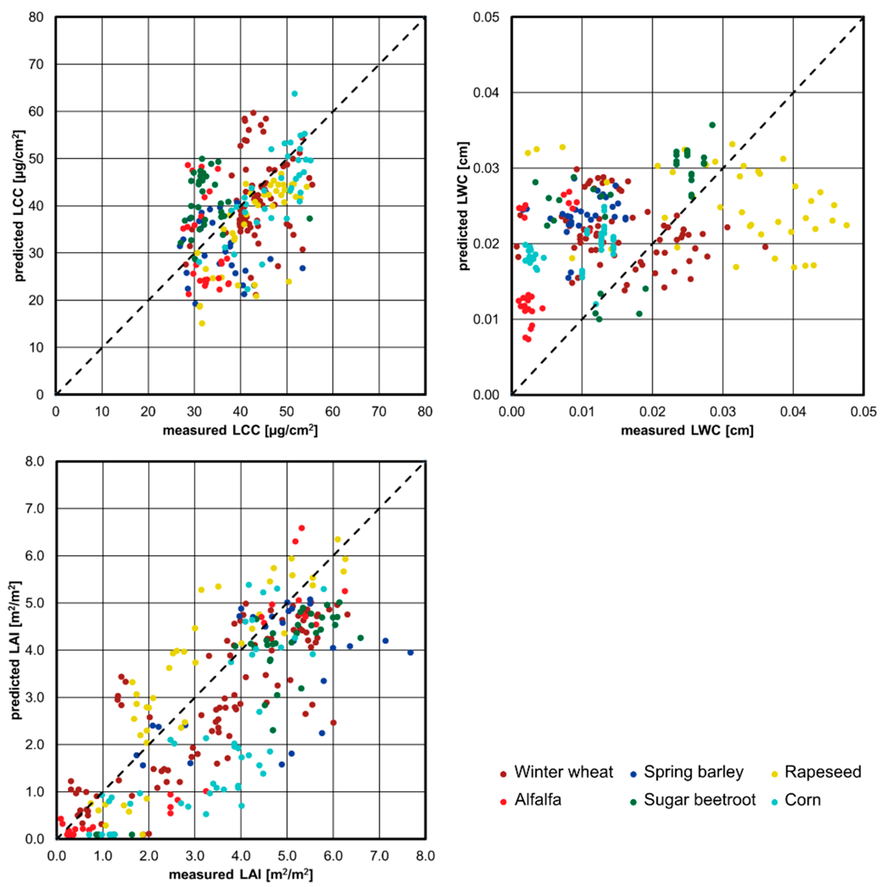
3.2.2. Crop Quantitative Product Inversion and Validation

Accuracy assessment of the biophysical retrievals was performed on the validation dataset of in situ measurements. For biophysical parameters retrieval, the closest Sentinel-2 scenes in terms of acquisition date (see Table 3 for list of Sentinel-2 scenes used) were always used. Figure 10 shows scatter plots comparing observed and retrieved LAI, LCC, and LWC values for all crops of interest.
For validation purposes, root mean square error (RMSE) and its relative magnitude (rRMSE) were calculated as the metrics of accuracy. Coefficient of determination (R2) and Pearson’s correlation coefficient (r), respectively, were chosen as the metrics for the prediction model’s variability and linearity of the relationship between simulations and reference in situ data. The values of these metrics at the level of individual crops and individual field campaigns are given in Table 5 and Table 6, respectively. Among the three retrieved crop parameters, the LAI estimations perform relatively the best. Pearson’s correlation coefficient for LAI retrieval was 0.80 (R2 = 0.63), total RMSE was 1.32, and the corresponding rRMSE was 37%. The retrieved LCC values show a total RMSE of 9.88 μg/cm2 (rRMSE = 25%) and thus exhibit the lowest relative error among all three studied parameters. However, significant relationship between simulations and reference in situ data were achieved only for three crops (corn, r = 0.69, R2 = 0.48; winter rapeseed, r = 0.66, R2 = 0.43; winter cereals, r = 0.41, R2 = 0.17), while the correlation for the remaining three crops was weak (spring cereals, r = 0.06, R2 = 0.00; fodder crops, r = -0.28, R2 = 0.08; sugar beetroot, r = 0.04, R2 = 0.00). Retrieval of LWC is the most uncertain. The errors achieved are really high (RMSE = 0.0124 cm; rRMSE = 78%) and also the strength of the relationship between simulated and reference in situ data is insufficient. Examples of annual changes in the values of estimated biophysical parameters are shown in Figure A4 (LAI), Figure A5 (LCC) and Figure A6 (LWC).

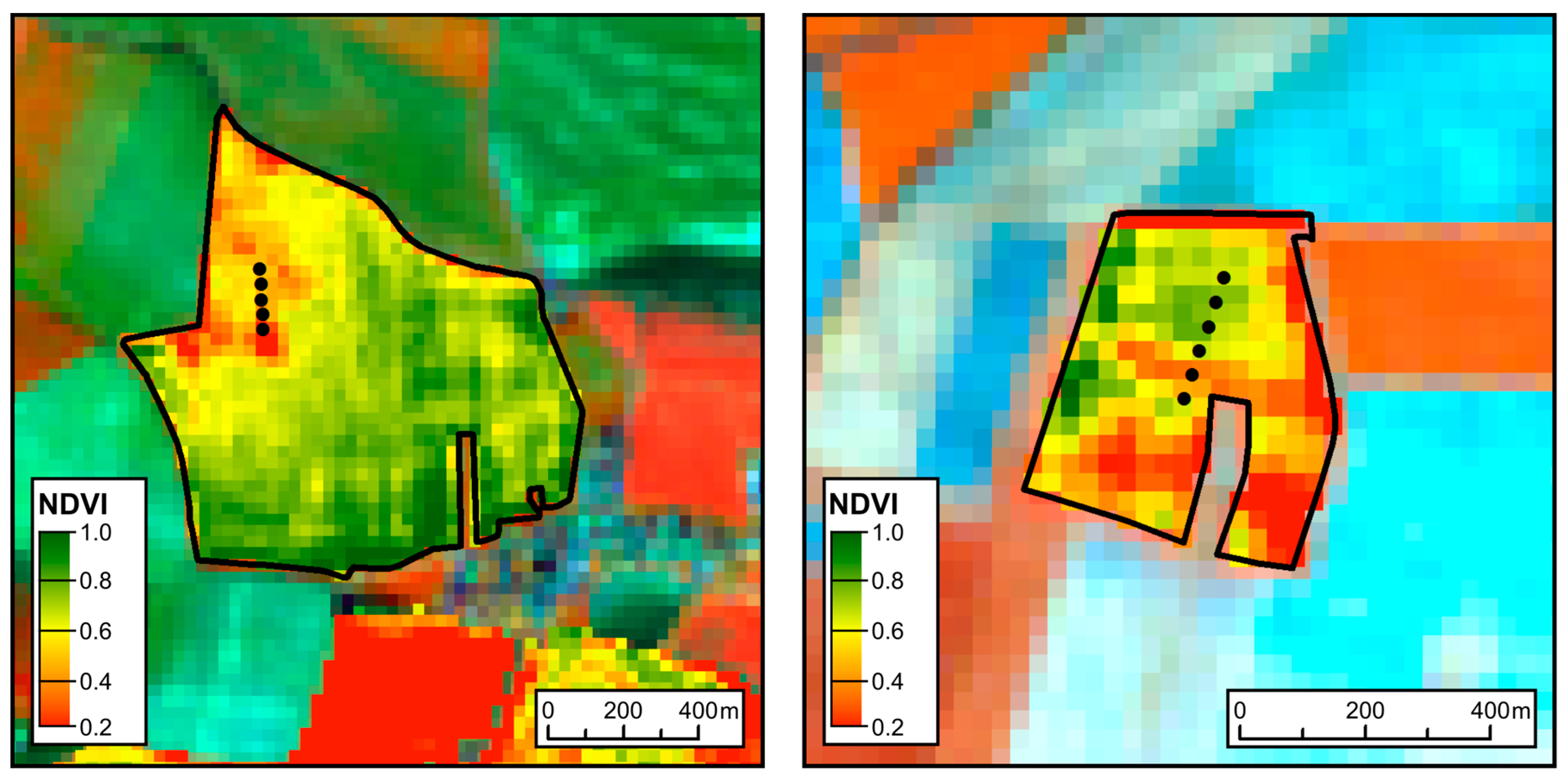
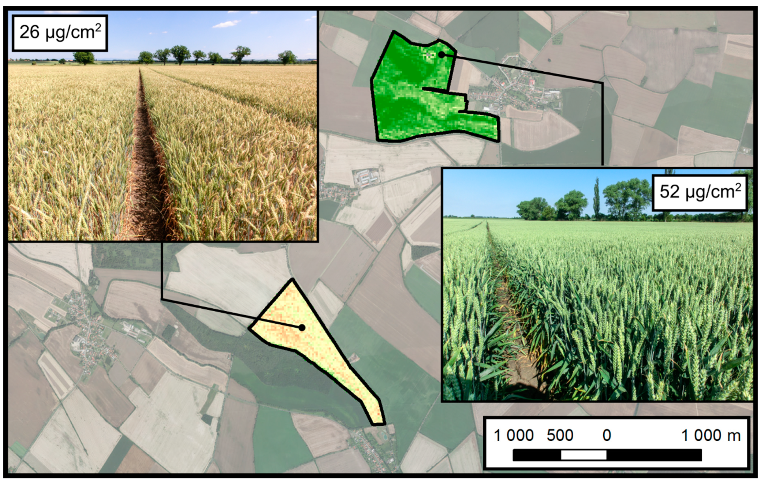
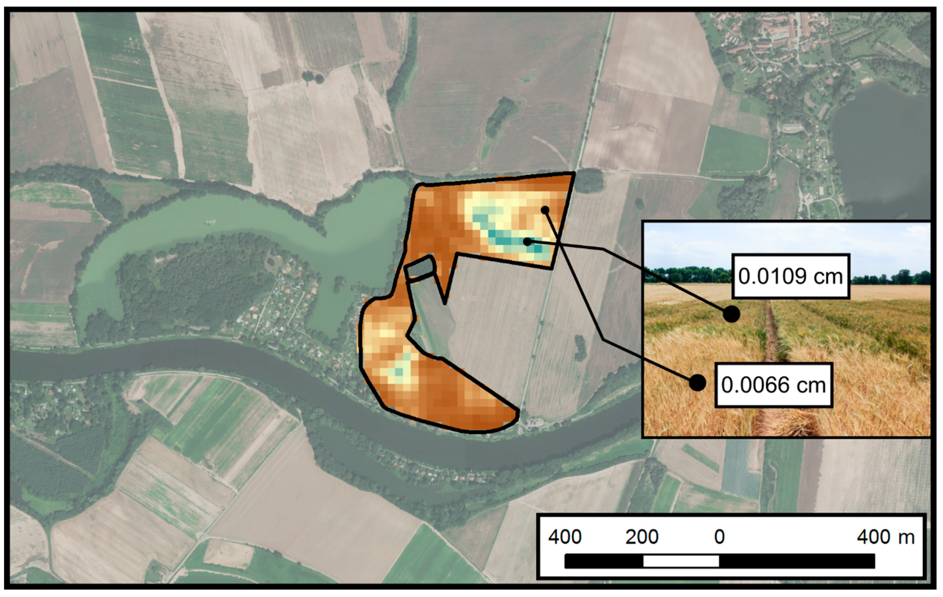
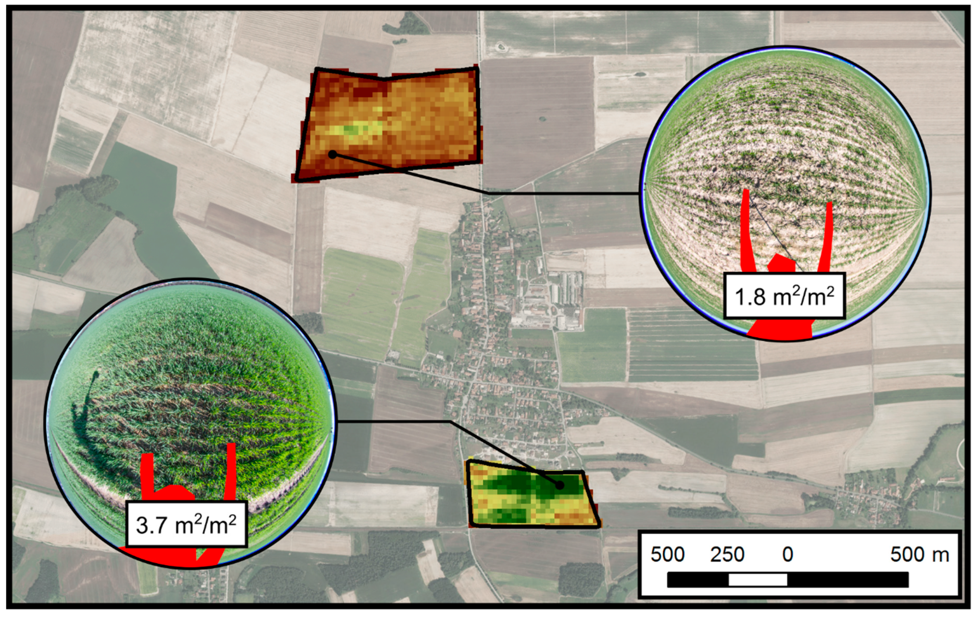
3.3. Practical Examples and Designing of Crop Management Zones

The entire workflow of quantitative estimation of canopy biophysics was applied to the time series of Sentinel−2 data acquired during the 2017 and 2018 vegetation seasons covering the farms where in-situ data were collected in the same time period. Representative samples were selected to show key features of the output products and to demonstrate their potential use in agriculture management.
Figure 11 shows an example of LCC estimation for winter wheat canopies in the preharvest period (the data were acquired on 20 June 2017). The two sample parcels exhibit significantly different values of LCC corresponding to the difference in wheat maturity (26 μg/cm2 and brownish status for late maturity compared to 52 μg/cm2 and greenish status for early maturity). The chlorophyll content plays an important role in harvest management, helping to estimate maturity and determine the optimal harvest date.
Figure 12 gives an example of LWC estimation for spring barley canopies. Significantly different canopy water content patterns in barley canopy can be seen in the northern section compared to the rest of the given parcel. The observed difference in vegetation characteristics—green canopy exhibiting almost double the LWC (0.0109 cm) compared to the brown canopy (0.0066 cm) on most of the field—is determined by the presence of the remnant of river (now filled by fluvial sediments). The old river remnant creates a local topographic sink with wet soil conditions compared to the rest of the area. Such local difference in soil wetness influences the biophysical characteristics of the spring barley that is being cultivated here. LWC can be used not only to monitor actual water nutrition of the crop canopies, but also, similarly as is LCC, for assessing crop maturity.
A third example, shown in Figure 13, presents an LAI estimation applied on winter wheat canopies at the beginning of the growing season (data acquired 1 April 2017). The two parcels exhibit significantly different canopy density that is clearly reflected by the differences in retrieved LAI values. Information on canopy density and other conditions can be useful for variable application of fertilizers at the beginning of the growing season. Continuous monitoring of the LAI estimation can then be used to assess increase in vegetation biomass, which may in turn serve as an input to yield estimation models.

4. Discussion

4.1. Sentinel-2 Images for the Determination of Crop Biophysics

Compared to more complex land cover types, such as forests, the agricultural canopies are relatively homogeneous. This allowed direct comparison of in situ measured TOC reflectance against Sentinel-2 TOC reflectance observations after applying the sensor response function of Sentinel-2 satellite on hyperspectral ground measurements [41]. A strong relationship (R2 > 0.7) for six spectral bands and also a significant relationship (R2 = 0.57, 0.63 and 0.68) for the other three bands were achieved, so Sentinel-2 images may be considered as constituting a suitable data source for retrieval of the biophysical characteristics of agricultural crops.

4.2. In Situ Data Collection

A database of in situ crop biophysical characteristics was used for representative parametrization of radiative transfer model and robust validation of its inverted parameters. The measurements of LAI were taken using two different instruments (DHP and SunScan). Each method is suitable for different crop types and their phenological stages. Because the inversion of LAI from DHP images is based on the relationships between estimated angular gap fractions and canopy structure, it is more suited for low-growing crops (e.g., sugar beet, alfalfa) or for early development stages of crops. In cases of tall dense canopies, leaves may be mutually shaded and clumped, resulting in underestimation of LAI. In such cases, the SunScan device is preferred since it determines the direct transmittance of solar radiation through the canopy. On the other hand, the SunScan measurements of canopy transmittance for low and sparse canopies may lead to the underestimations of LAI due to the size of the plant.
The parameterization of the PROSAIL model also included setting of the crop-specific leaf structural parameter (N). These were obtained from the inversion of the PROSPECT model against measured leaf spectra with known model input biochemical parameters. The retrieved N values were then compared to those included in the LOPEX-93 database. Our results show good agreement of retrieved N number with those provided in the LOPEX-93 database: alfalfa 1.53 ± 0.12 vs. 1.61 ± 0.14, sugar beet 1.67 ± 0.19 vs. 1.75 ± 0.14, and corn 1.28 ± 0.09 vs. 1.41 ± 0.11 [33].
In our study, we used a fixed value of N for each crop. Because the N parameter describes the leaf thickness, the exact N value may vary during the crop growth cycle as the leaves develop. On the other hand, the crops addressed in this study are all annual plants with short cycles, thus we assume that the changes in leaf thickness will be relatively small. Although we consider quantification of the N number to be representative for this study, more research on the seasonal changes in leaf biochemical (e.g., chlorophylls and leaf water content) and structural (e.g., leaf thickness) are needed to further reduce model uncertainties.

4.3. Satellite-Based Crop Biophysics Validation

Direct validation of remotely sensed crop parameters is a widely used method for assessing the uncertainties of retrieved products. Nevertheless, the in situ data should not be considered as a ground truth with no internal uncertainties. Each of the instruments (Delta-T SunScan and DHP for LAI assessment, Force-A Dualex for LCC, laboratory scales and desktop scanner for LWC measurements) has their individual accuracies and error sources. In the case of LWC, the overall error is even a combination of several instruments. As a result, such validation efforts are rather a comparison of two independent methods for retrieving crop biophysical parameters.
Direct validation of PROSAIL model retrievals showed the highest accuracy for LAI (r = 0.80, R2 = 0.63, RMSE = 1.32 m2/m2, and rRMSE = 37%). The best relative accuracy of all three calculated biophysical parameters was achieved for the LCC (rRMSE = 25%). However, the correlations with the in situ measurements were crop-specific (corn, r = 0.69, R2 = 0.48; winter rapeseed, r = 0.66, R2 = 0.43; winter cereals, r = 0.41, R2 = 0.17), while the correlation for the remaining crops was not significant. The poor performance of the LCC retrieval for some of the crops may be caused by the relatively low range of measured in-situ values. For example, the RMSE of LCC retrieval for most of the crops was higher than the standard deviation of in situ LCC measurements.
Retrieval of LWC, is technically feasible, but the total retrieval accuracy against in situ data was rather poor (r = 0.33, R2 = 0.11, RMSE = 0.0124 cm, and rRMSE = 78%). On the other hand, determination of LWC from in situ data might be also affected by individual errors of the instruments used for its quantification. The in situ LWC exhibits high variability across campaigns. We note that the relationship between retrieved and reference in situ data for individual campaigns was often much higher (e.g., r = 0.70, 0.85, and 0.93, respectively, for the campaigns dated 20–21 June 2017, 4–5 April 2018, and 21 June 2018).

4.4. Discussion of the Results Relative to the Literature

Results obtained in our study were also compared against previous studies focused on crop monitoring using high-resolution satellite multispectral data using similar methodological approaches (i.e., inversion of radiative transfer model). It should be noted that the retrieval accuracy is always specific to a given crop and its phenological phase. Therefore, the comparison should be made only at the individual crop level while taking into account the development stage of crop and collected in situ data.
We observed satisfactory results of model inversion for crop LAI and LCC, while the inversion of LWC was of poor quality. This is in agreement with the previous studies [2,26]. Leaf area index is the most frequently retrieved crop biophysical parameter. As reported in [9], the accuracy of LAI retrieval for winter wheat was RMSE = 1.53 m2/m2, for the same crop, [42] reports RMSE = 0.43 m2/m2, [43] reports RMSE = 0.56 m2/m2, [44] reports RMSE = 0.62 m2/m2, [45] reports RMSE between 0.4–0.6 m2/m2 and [46] reports RMSE = 0.55 m2/m2. Our RMSE for winter wheat was 1.13 m2/m2, which is in line with these reported values. The validation of other crops of interest (alfalfa, sugar beet, and corn) is reported by [14] as RMSE = 1.39 m2/m2, 2.24 m2/m2, and 1.43 m2/m2 for alfalfa, sugar beet, and corn, respectively. In our study, we achieved comparable accuracies (alfalfa: RMSE = 1.50 m2/m2, sugar beet: RMSE = 1.13 m2/m2, and corn: RMSE = 1.72 m2/m2).
In previous studies, the chlorophyll content is frequently retrieved on the canopy level as LAI × LCC. Direct comparison of leaf chlorophyll content (as performed in our study) is shown, for instance, by [9]. They report the RMSE = 12.69 μg/cm2 for winter wheat. A similar RMSEs for winter wheat are also presented by [47] (RMSE = 11.86 μg/cm2 for 2014 season and 7.17 μg/cm2 for 2014/2015 season), but for the data with higher spectral resolution corresponding to the future EnMap mission. In [43] was obtained an RMSE of 9.06 μg/cm2 for winter wheat retrieved from IRS LISS-3 sensor. Wheat and corn LCC was retrieved by [48] for leaf level (RMSE = 9.45–13.62 μg/cm2) and Landsat-8 level (RMSE = 16.18 μg/cm2). In our study we achieved the RMSE = 9.59 μg/cm2, which is again well in line with the previous studies.
There are only a few studies focusing on the retrieval of LWC, all of them showed rather poor retrieval accuracies. These include work by [49] on the retrieval of LWC for grasses, shrubs and forests. Here the authors showed high rRMSE of grassess (rRMSE between 100 and 160%), compared to forests (rRMSE around 50%) and shrubs (rRMSE around 80%). Similarly, [43] reported poor performance of LWC retrieval for wheat, compared to LAI and LCC retrievals. In our study, the validation of LWC was also poor, exhibiting high rRMSE (78%) across studied crops and their development stages. We thus conclude, that the only two retrievable crop parameters of interest are LAI and LCC.

5. Conclusions

Sentinel-2 multispectral imagery provides sufficient data for monitoring the health condition of agricultural crop canopy. Its main advantage is the imagery’s high temporal resolution (ca 5 days). This makes it possible to monitor even very gradual changes in the state of vegetation. By applying a physics based, transferable retrieval method, Sentinel-2 data can be a robust source of information for estimating crop biophysical indicators. The main advantage over using a simple empirical approach can be seen in the fact that it is based on well-defined physical laws which are not site and time specific. On the other hand, each model represents some degree of generalization that can have some effect on the obtained results. To ensure robustness of the estimated biophysical parameters, it is needed to have a collection of reference in situ data obtained for different phenological phases of the crop canopies which can be used for proper parameterization of the considered radiative transfer model.
One such method, based on the inversion of biophysical parameters using the PROSAIL model, look-up tables, and artificial neural network, was introduced in this study. The procedure involved the calculation of three biophysical parameters (leaf chlorophyll content [LCC], leaf water content [LWC], and leaf area index [LAI]) on six crops of interest (winter wheat, spring barley, winter rapeseed, alfalfa, corn, and sugar beet).
It was found that good results were achieved for LAI (r = 0.80, R2 = 0.63, RMSE = 1.32 m2/m2, and rRMSE = 37%). Satisfactory results in terms of absolute and relative accuracy were also achieved with the LCC (RMSE = 9.88 μg/cm2, and rRMSE = 25%). However, significant correlations with in situ measurements were obtained only for corn, winter wheat and winter rapeseed. Weaker results in terms of the strength of the relationship between retrieved and reference in situ data could be caused by relatively small variability of LCC in situ measurement values. Results of LWC retrieval were found as insufficient (r = 0.33, R2 = 0.11, RMSE = 0.0124 cm, and rRMSE = 78%). Such weak retrieval results, however, could have been caused by error from the relatively complex calculation of in situ values. On the other hand, even the LWC estimation in previous studies did not lead to better results.
The main benefit of the presented study is that it outlines a complete procedure for biophysical monitoring of agricultural crops usable in pursuing the principles of precision agriculture. The study demonstrates the potential of Sentinel-2 data together with radiative transfer modeling to support such agricultural management interventions as selective fertilization and irrigation, as well as harvest planning.

Author Contributions

Conceptualization, J.M. and P.L.; Data Curation, J.T., J.M. and P.L.; Formal Analysis, J.T., J.M. and P.L.; Funding Acquisition, J.M. and P.L.; Investigation, J.M. and P.L.; Methodology, J.M. and P.L.; Project Administration, J.M. and P.L.; Resources, J.M. and P.L.; Software, J.T.; Supervision, J.M. and P.L.; Validation, J.T.; Visualization, J.M.; Writing—Original Draft, J.T., J.M. and P.L. All authors have read and agreed to the published version of the manuscript.

Funding

This research was funded by the Technology Agency of the Czech Republic, project TH02030248: Use of Copernicus satellite data for an effective monitoring of a status and management of selected agricultural crops. Petr Lukeš was also supported by the project “SustES-Adaptation strategies for sustainable ecosystem services and food security under adverse environmental conditions” (CZ.02.1.01/0.0/0.0/16_019/0000797).

Institutional Review Board Statement

Not applicable.

Informed Consent Statement

Not applicable.

Acknowledgments

We would like to thank the agronomists of the cooperating farms for their support in selecting and allowing access to agricultural parcels in order to in situ data collection, namely Martina Martincová (Poděbradská Blata a.s.) and Jiří Hlaváček (Pěstitel Stratov s.r.o.). We would also like to thank all those who contributed to the realization of field campaigns, namely Jan Foldyna, Karel Klem (GCRI), Lukáš Fajmon (GCRI), Tomáš Purket (GCRI), Rahul Raj (GCRI), Lucie Brabcová (Gisat Ltd.), Kateřina Tučková (Gisat Ltd.) and Markéta McEwan (Gisat Ltd.).

Conflicts of Interest

The authors declare no conflict of interest.

Appendix A

Table A1. Summary of the in-situ measured values of selected biophysical variables (LCC—leaf chlorophyll content, LWC—leaf water content, SLW—dry matter content (specific leaf weight) and LAI—leaf area index).
CropDatasetVariableLCC [µg/cm2]LWC [cm]SLW [g/cm2]LAI
Winter cereals
(winter wheat)
calibration
n = 84
MIN2.20.00050.00030.8
MEAN42.20.01550.00443.9
MAX55.00.02880.00726.0
STD10.90.00720.00171.3
validation
n = 96
MIN2.20.00070.00100.3
MEAN41.80.01610.00473.5
MAX59.40.03600.02236.3
STD11.60.00710.00271.7
Spring cereals
(spring barley)
calibration
n = 31
MIN2.70.00170.00050.3
MEAN32.00.00950.00314.2
MAX48.10.01530.00596.8
STD9.70.00350.00191.8
validation
n = 29
MIN4.10.00160.00040.2
MEAN34.30.01020.00324.2
MAX53.40.01620.00697.7
STD8.30.00370.00172.0
Winter rapeseedcalibration
n = 56
MIN26.10.00370.00030.4
MEAN42.70.03240.00573.4
MAX55.30.14230.02808.5
STD6.50.01880.00432.6
validation
n = 51
MIN26.30.00220.00060.7
MEAN41.60.03010.00563.7
MAX54.30.05010.00988.6
STD7.20.01180.00292.1
Fodder crops
(alfalfa)
calibration
n = 29
MIN24.00.00110.00370.1
MEAN31.50.00380.00532.7
MAX39.00.01170.00767.2
STD3.80.00310.00082.4
validation
n = 28
MIN23.40.00100.00350.1
MEAN31.60.00360.00512.8
MAX37.30.01110.006910.2
STD3.60.00290.00082.6
Sugar beetrootcalibration
n = 26
MIN25.30.00470.00210.9
MEAN32.20.01120.00574.4
MAX53.70.03530.00766.7
STD5.10.00770.00121.7
validation
n = 36
MIN25.70.00330.00190.9
MEAN32.00.01180.00584.6
MAX55.00.02850.00826.6
STD4.90.00620.00121.5
Corncalibration
n = 27
MIN33.90.00120.00410.7
MEAN50.40.00840.00583.6
MAX60.20.01440.01255.8
STD6.80.00530.00161.4
validation
n = 44
MIN31.00.00190.00080.7
MEAN49.20.00350.00573.4
MAX59.40.01190.00795.8
STD6.90.00240.00121.4
Figure A1. Location of agricultural parcels where campaigns were conducted together with true color Sentinel-2 images for the “early season” (6 April 2018; (A)), “mid season” (14 May 2018; (B)) and “late season” (19 August 2018; (C)).
Remotesensing 13 03659 g0a1
Figure A2. Sentinel-2 and in situ measured spectra for the different development stages of crops of interest.
Remotesensing 13 03659 g0a2
Figure A3. Sentinel-2 spectra and PROSAIL simulations for the different development stages of crops of interest.
Remotesensing 13 03659 g0a3
Figure A4. Temporal changes in estimated leaf area index (LAI) values for all six crops of interest demonstrated using Q0.25, Q0.50, and Q0.75 quantiles.
Remotesensing 13 03659 g0a4
Figure A5. Temporal changes in estimated leaf chlorophyll content (LCC) values for all six crops of interest demonstrated using Q0.25, Q0.50, and Q0.75 quantiles.
Remotesensing 13 03659 g0a5
Figure A6. Temporal changes in estimated leaf water content (LWC) values for all six crops of interest demonstrated using Q0.25, Q0.50, and Q0.75 quantiles.
Remotesensing 13 03659 g0a6

References

  1. Jones, H.G.; Vaughan, R.A. Remote Sensing of Vegetation: Principles, Techniques, and Applications; Oxford University Press: Oxford, UK, 2010; 353p. [Google Scholar]
  2. Weiss, M.; Jacob, F.; Duveiller, G. Remote sensing for agricultural applications: A meta-review. Remote Sens. Environ. 2020, 236, 111402. [Google Scholar] [CrossRef]
  3. Sishodia, R.P.; Ray, R.L.; Singh, S.K. Applications of remote sensing in precision agriculture: A review. Remote Sens. 2020, 12, 3136. [Google Scholar] [CrossRef]
  4. Holman, F.H.; Riche, A.B.; Michalski, A.; Castle, M.; Wooster, M.J.; Hawkesford, M.J. High throughput field phenotyping of wheat plant height and growth rate in field plot trials using UAV based remote sensing. Remote Sens. 2016, 8, 1031. [Google Scholar] [CrossRef]
  5. Ali, I.; Greifeneder, F.; Stamenkovic, J.; Neumann, M.; Notarnicola, C. Review of machine learning approaches for biomass and soil moisture retrievals from remote sensing data. Remote Sens. 2015, 7, 16398–16421. [Google Scholar] [CrossRef] [Green Version]
  6. Chen, D.; Huang, J.; Jackson, T.J. Vegetation water content estimation for corn and soybeans using spectral indices derived from MODIS near- and short-wave infrared bands. Remote Sens. Environ. 2005, 98, 225–236. [Google Scholar] [CrossRef]
  7. Gitelson, A.A.; Viña, A.; Ciganda, V.; Rundquist, D.C.; Arkebauer, T.J. Remote estimation of canopy chlorophyll content in crops. Geophys. Res. Lett. 2005, 32, 1–4. [Google Scholar] [CrossRef] [Green Version]
  8. Delloye, C.; Weiss, M.; Defourny, P. Retrieval of the canopy chlorophyll content from Sentinel-2 spectral bands to estimate nitrogen uptake in intensive winter wheat cropping systems. Remote Sens. Environ. 2018, 216, 245–261. [Google Scholar] [CrossRef]
  9. Xie, Q.; Dash, J.; Huete, A.; Jiang, A.; Yin, G.; Ding, Y.; Peng, D.; Hall, C.C.; Brown, L.; Shi, Y.; et al. Retrieval of crop biophysical parameters from Sentinel-2 remote sensing imagery. Int. J. Appl. Earth Obs. Geoinf. 2019, 80, 187–195. [Google Scholar] [CrossRef]
  10. Banerjee, K.; Krishnan, P.; Mridha, N. Application of thermal imaging of wheat crop canopy to estimate leaf area index under different moisture stress conditions. Biosyst. Eng. 2018, 166, 13–27. [Google Scholar] [CrossRef]
  11. Pineda, M.; Barón, M.; Pérez-Bueno, M.L. Thermal imaging for plant stress detection and phenotyping. Remote Sens. 2021, 13, 68. [Google Scholar] [CrossRef]
  12. Harfenmeister, K.; Spengler, D.; Weltzien, C. Analyzing temporal and spatial characteristics of crop parameters using Sentinel-1 backscatter data. Remote Sens. 2019, 11, 1569. [Google Scholar] [CrossRef] [Green Version]
  13. Baker, R.E.; Peña, J.M.; Jayamohan, J.; Jérusalem, A. Mechanistic models versus machine learning, a fight worth fighting for the biological community? Biol. Lett. 2018, 14, 20170660. [Google Scholar] [CrossRef] [PubMed]
  14. Atzberger, C.; Richter, K. Spatially constrained inversion of radiative transfer models for improved LAI mapping from future Sentinel-2 imagery. Remote Sens. Environ. 2012, 120, 208–218. [Google Scholar] [CrossRef]
  15. Johnson, M.D.; Hsieh, W.W.; Cannon, A.J.; Davidson, A.; Bédard, F. Crop yield forecasting on the Canadian Prairies by remotely sensed vegetation indices and machine learning methods. Agric. For. Meteorol. 2016, 218–219, 74–84. [Google Scholar] [CrossRef]
  16. Garbulsky, M.F.; Peñuelas, J.; Gamon, J.; Inoue, Y.; Filella, I. The photochemical reflectance index (PRI) and the remote sensing of leaf, canopy and ecosystem radiation use efficiencies. A review and meta-analysis. Remote Sens. Environ. 2011, 115, 281–297. [Google Scholar] [CrossRef]
  17. de Leeuw, J.; Vrieling, A.; Shee, A.; Atzberger, C.; Hadgu, K.M.; Biradar, C.M.; Keah, H.; Turvey, C. The potential and uptake of remote sensing in insurance: A review. Remote Sens. 2014, 6, 10888–10912. [Google Scholar] [CrossRef] [Green Version]
  18. Jin, Z.; Prasad, R.; Shriver, J.; Zhuang, Q. Crop model- and satellite imagery-based recommendation tool for variable rate N fertilizer application for the US Corn system. Precis. Agric. 2017, 18, 779–800. [Google Scholar] [CrossRef]
  19. Rouse, J.W.; Hass, R.H.; Schell, J.A.; Deering, D.W. Monitoring vegetation systems in the Great Plains with ERTS. Nasa ERTS Symp. 1973, 351, 309–313. [Google Scholar]
  20. Oregon® 300|Garmin Support. Available online: https://support.garmin.com/en-US/?partNumber=010-00697-01&tab=manuals (accessed on 13 October 2020).
  21. Goulas, Y.; Cerovic, Z.G.; Cartelat, A.; Moya, I. Dualex: A new instrument for field measurements of epidermal ultraviolet absorbance by chlorophyll fluorescence. Appl. Opt. 2004, 43, 4488–4496. [Google Scholar] [CrossRef]
  22. Cerovic, Z.G.; Masdoumier, G.; Ghozlen, N.B.; Latouche, G. A new optical leaf-clip meter for simultaneous non-destructive assessment of leaf chlorophyll and epidermal flavonoids. Physiol. Plant. 2012, 146, 251–260. [Google Scholar] [CrossRef]
  23. Webb, N.; Nicholl, C.; Wood, J.; Potter, E. SunScan Manual Version 3.3; Delta-T Devices Ltd.: Cambridge, UK, 2016; pp. 1–82. [Google Scholar]
  24. Weiss, M.; Baret, F. Can_Eye V6.4.91 User Manual; INRA: Paris, France, 2017; p. 56. [Google Scholar]
  25. ASD FieldSpec® 4 Hi-Res: Espectroradiómetro de Alta Resolución|Malvern Panalytical. Available online: https://www.malvernpanalytical.com/es/products/product-range/asd-range/fieldspec-range/fieldspec4-hi-res-high-resolution-spectroradiometer?creative=315830988458&keyword=&matchtype=b&network=g&device=c&gclid=EAIaIQobChMInNybno746gIVx4TVCh3XaABcEAAYASAAEgIa (accessed on 13 October 2020).
  26. Berger, K.; Atzberger, C.; Danner, M.; D’Urso, G.; Mauser, W.; Vuolo, F.; Hank, T. Evaluation of the PROSAIL model capabilities for future hyperspectral model environments: A review study. Remote Sens. 2018, 10, 85. [Google Scholar] [CrossRef] [Green Version]
  27. Jacquemoud, S.; Verhoef, W.; Baret, F.; Bacour, C.; Zarco-Tejada, P.J.; Asner, G.P.; François, C.; Ustin, S.L. PROSPECT + SAIL models: A review of use for vegetation characterization. Remote Sens. Environ. 2009, 113, S56–S66. [Google Scholar] [CrossRef]
  28. Weiss, M.; Baret, F.; Myneni, R.B.; Pragnère, A.; Knyazikhin, Y. Investigation of a model inversion technique to estimate canopy biophysical variables from spectral and directional reflectance data. Agronomie 2000, 20, 3–22. [Google Scholar] [CrossRef]
  29. Feret, J.B.; François, C.; Asner, G.P.; Gitelson, A.A.; Martin, R.E.; Bidel, L.P.; Ustin, S.L.; le Maire, G.; Jacquemoud, S. PROSPECT-4 and 5: Advances in the leaf optical properties model separating photosynthetic pigments. Remote Sens. Environ. 2008, 112, 3030–3043. [Google Scholar] [CrossRef]
  30. Jacquemoud, S.; Baret, F. PROSPECT: A model of leaf optical properties spectra. Remote Sens. Environ. 1990, 34, 75–91. [Google Scholar] [CrossRef]
  31. Verhoef, W. Light scattering by leaf layers with application to canopy reflectance modeling: The SAIL model. Remote Sens. Environ. 1984, 16, 125–141. [Google Scholar] [CrossRef] [Green Version]
  32. Nieto, H. GitHub-Hectornieto/pyPro4Sail: ProspectD and 4SAIL Radiative Transfer Models for Simulating the Transmission of Radiation in Leaves and Canopies. Available online: https://github.com/hectornieto/pyPro4Sail (accessed on 6 December 2017).
  33. Hosgood, B.; Jacquemoud, S.; Andreoli, G.; Verdebout, J.; Pedrini, G.; Schmuck, G. Leaf Optical Properties EXperiment 93 (LOPEX93); Report EUR 16095 EN; Joint Research Centre, European Commission Institute for Remote Sensing Applications: Luxembourg, 1994; p. 11. [Google Scholar]
  34. ESA Sentinel 2 Document Library-Sentinel-2 Spectral Response Functions (S2-SRF). Available online: https://earth.esa.int/web/sentinel/user-guides/sentinel-2-msi/document-library/-/asset_publisher/Wk0TKajiISaR/content/sentinel-2a-spectral-responses (accessed on 3 April 2021).
  35. Jacquemoud, S. Inversion of the PROSPECT + SAIL canopy reflectance model from AVIRIS equivalent spectra: Theoretical study. Remote Sens. Environ. 1993, 44, 281–292. [Google Scholar] [CrossRef]
  36. ESA Sen2Cor 2.2.5. Available online: https://step.esa.int/main/snap-supported-plugins/sen2cor/ (accessed on 30 July 2021).
  37. Richter, K.; Hank, T.B.; Vuolo, F.; Mauser, W.; D’Urso, G. Optimal exploitation of the sentinel-2 spectral capabilities for crop leaf area index mapping. Remote Sens. 2012, 4, 561–582. [Google Scholar] [CrossRef] [Green Version]
  38. Raschka, S. Python Machine Learning: Unlock Deeper Insights into Machine Learning with This Vital Guide to Cutting-Edge Predictive Analytics; Packt Publishing Ltd.: Birmingham, UK, 2015; ISBN 9781783555130. [Google Scholar]
  39. Escobar-Gutiérrez, A.J.; Combe, L. Senescence in field-grown maize: From flowering to harvest. F. Crop. Res. 2012, 134, 47–58. [Google Scholar] [CrossRef]
  40. Schlemmer, M.R.; Francis, D.D.; Shanahan, J.F.; Schepers, J.S. Remotely measuring chlorophyll content in corn leaves with differing nitrogen levels and relative water content. Agron. J. 2005, 97, 106–112. [Google Scholar] [CrossRef] [Green Version]
  41. Wang, Q.; Li, P. Canopy vertical heterogeneity plays a critical role in reflectance simulation. Agric. For. Meteorol. 2013, 169, 111–121. [Google Scholar] [CrossRef]
  42. Pan, H.; Chen, Z.; Ren, J.; Li, H.; Wu, S. Modeling Winter Wheat Leaf Area Index and Canopy Water Content with Three Different Approaches Using Sentinel-2 Multispectral Instrument Data. IEEE J. Sel. Top. Appl. Earth Obs. Remote Sens. 2019, 12, 482–492. [Google Scholar] [CrossRef]
  43. Sehgal, V.K.; Chakraborty, D.; Sahoo, R.N. Inversion of radiative transfer model for retrieval of wheat biophysical parameters from broadband reflectance measurements. Inf. Process. Agric. 2016, 3, 107–118. [Google Scholar] [CrossRef] [Green Version]
  44. Herrmann, I.; Pimstein, A.; Karnieli, A.; Cohen, Y.; Alchanatis, V.; Bonfil, D.J. LAI assessment of wheat and potato crops by VENμS and Sentinel-2 bands. Remote Sens. Environ. 2011, 115, 2141–2151. [Google Scholar] [CrossRef]
  45. Richter, K.; Atzberger, C.; Vuolo, F.; D’Urso, G. Evaluation of Sentinel-2 Spectral Sampling for Radiative Transfer Model Based LAI Estimation of Wheat, Sugar Beet, and Maize. IEEE J. Sel. Top. Appl. Earth Obs. Remote Sens. 2011, 4, 458–464. [Google Scholar] [CrossRef]
  46. Dorigo, W.A. Improving the robustness of cotton status characterisation by radiative transfer model inversion of multi-angular CHRIS/PROBA data. IEEE J. Sel. Top. Appl. Earth Obs. Remote Sens. 2012, 5, 18–29. [Google Scholar] [CrossRef]
  47. Danner, M.; Berger, K.; Wocher, M.; Mauser, W.; Hank, T. Retrieval of Biophysical Crop Variables from Multi-Angular Canopy Spectroscopy. Remote Sens. 2017, 9, 726. [Google Scholar] [CrossRef] [Green Version]
  48. Croft, H.; Arabian, J.; Chen, J.M.; Shang, J.; Liu, J. Mapping within-field leaf chlorophyll content in agricultural crops for nitrogen management using Landsat-8 imagery. Precis. Agric. 2020, 21, 856–880. [Google Scholar] [CrossRef] [Green Version]
  49. Casas, A.; Riaño, D.; Ustin, S.L.; Dennison, P.; Salas, J. Estimation of water-related biochemical and biophysical vegetation properties using multitemporal airborne hyperspectral data and its comparison to MODIS spectral response. Remote Sens. Environ. 2014, 148, 28–41. [Google Scholar] [CrossRef]
Figure 1. Typical NDVI profiles (extracted from series of Sentinel-2 data) of the agricultural crops considered in this study characterizing temporal changes of crop canopies during the growing season. Reference in situ data were collected during 8 field campaigns A (29–31 March 2017); B (17–19 May 2017), C (19–21 June 2017), D (4–5 April 2018), E (27–30 April 2018), F (21 May 2018), G (20–21 June 2018), and H (26 July 2018). Collected measurements were further divided into calibration/validation data subsets (203 calibration/188 validation points in 2017; 124 calibration/144 validation points in 2018). DOY (day-of-year) stands for the ordinal number of the day in the given year (i.e., 1.1. = 1, 2.1. = 2…31.12. = 365 etc.).
Remotesensing 13 03659 g001
Figure 2. Selection of in situ transects. The latest cloud-free scene acquired before the date of an in situ sampling campaign (in this case 16 March 2017) was used to calculate a normalized difference vegetation index (NDVI) product. Spatial gradients of NDVI (assumed to describe spatial heterogeneity of canopy characteristics) were used for locating the sampling transect.
Remotesensing 13 03659 g002
Figure 3. Sampling scheme for digital hemispherical photography. Shown are a sampling reference point (blue) and eight DHP acquisition spots covering the corresponding Sentinel-2 pixel area (20 × 20 m).
Remotesensing 13 03659 g003
Figure 4. Relationship between leaf area index values extracted from digital hemispherical photography using CanEye software (x-axis) and measured by SunScan device (y-axis).
Remotesensing 13 03659 g004
Figure 5. Scatter plots over Sentinel-2 spectral bands between Sentinel-2 observations and the canopy-level spectra measured in situ at sample points.
Remotesensing 13 03659 g005
Figure 6. Empirical distribution functions of LIDFa, LIDFb, and Hspot parameters for six crops of interest.
Remotesensing 13 03659 g006
Figure 7. Chlorophyll to water content relationship recorded in our in situ data, showing water content limits.
Remotesensing 13 03659 g007
Figure 8. Spectral signatures of oil rapeseed canopy in flowering phenological phase: reference Sentinel-2 spectra (red line), original PROSAIL simulation (blue line), and PROSAIL simulation modified with spectral mixing of green and yellow components (green line).
Remotesensing 13 03659 g008
Figure 9. Scatter plots over Sentinel-2 spectral bands between Sentinel-2 observations and PROSAIL simulations calculated for in situ sample points with known biophysical parameters.
Remotesensing 13 03659 g009
Figure 10. Scatter plots for biophysical parameters LAI, LCC, and LWC retrieved and measured in situ (validation data subset).
Remotesensing 13 03659 g010
Figure 11. Example of leaf chlorophyll content estimation for two winter wheat parcels demonstrating differences in current maturity status as of 20 June 2017.
Remotesensing 13 03659 g011
Figure 12. Example of leaf water content (LWC) estimation for a spring barley parcel. The remnant of river (now filled by fluvial sediments) is a local topographic sink with higher soil wetness that influences the LWC of the cultivated crops (20 June 2017).
Remotesensing 13 03659 g012
Figure 13. Example of leaf area index (LAI) estimation for two winter wheat parcels demonstrating differences in crop canopy status of the winter crops at the beginning of the new vegetation season (1 April 2017).
Remotesensing 13 03659 g013
Table 1. Values of ProSail inputs common for all six crops of interest. LCC = leaf chlorophyll content, CX = carotenoid content, LWC = leaf water content, LAI = leaf area index, SA = sun azimuth, SZ = sun zenith, OA = observer azimuth, OZ = observer zenith, SKYL = fraction of diffuse solar radiation.
LCCCXLWCLAISASZOAOZSKYL
min000.0005015025-00.2
max8080.078 (10)17070-00.2
dist.uniformuniformuniformuniform5° step5° stepFixfixfix
Table 2. ProSAIL inputs with different values for six crops of interest (SLW = specific leaf weight, N = leaf structural parameter, LIDFa, LIDFb and HSpot = leaf and canopy structure parameters).
SLWNLIDF_ALIDF_BHOTSPOT
minmaxdist.fixedminmaxdist.minnmaxdist.minmaxdist.
W. cereals0.00090.0197norm1.44−10emp.−11emp.0.010.5emp
S. cereals0.0010.0138norm1.57−10emp.−11emp.0.010.5emp
O. rapeseed0.00050.01uniform1.78−11emp.−11emp.0.50.5fix
S. beetroot0.0030.008norm1.67−10emp.−11emp.0.10.5emp
Alfalfa0.0030.008norm1.53−11emp.−11emp.00.5emp
Corn0.0030.008norm1.28−11emp.−11emp0.20.5emp
Table 3. Summary on in-situ data collection campaigns dates and the reference Sentinel-2 scenes.
In-Situ Campaign DateReference Sentinel-2 Scene Acquisition DateReference Sentinel-2 Scene Sun Geometry (SZ, SA)
29–31 March 20171.4.201746.8°, 161.4°
17–19 May 201714.5.2017 and 21.5.201732.2°, 163.7° and 31.2°, 158.4°
19–21 June201720.6.201728.5°, 154.5°
4–5 April 20186.4.201844.9°, 161.3°
27–30 April 201826.4.201837.8°, 160.8°
21 May201821.5.201831.2°, 158.5°
20–21 June 201820.6.201828.5°, 154.5°
26 July201828.7.201832.5°, 159.2°
Table 4. Summary of the in-situ measured values of selected biophysical variables (LCC—leaf chlorophyll content, LWC—leaf water content, SLW—specific leaf weight and LAI—leaf area index).
CropVariableLCC (µg/cm2)LWC (cm)SLW (g/cm2)LAI
Winter cereals
(winter wheat)
n = 180
MIN2.240.00050.00030.31
MEAN42.060.01570.00453.68
MAX59.350.03600.02236.31
STD11.240.00720.00221.56
Spring cereals
(spring barley)
n = 60
MIN2.660.00160.00040.24
MEAN33.120.00980.00314.19
MAX53.370.01620.00697.67
STD9.110.00360.00181.90
Winter rapeseed
n = 107
MIN26.290.00220.00300.61
MEAN43.190.03300.00713.45
MAX55.300.14230.02808.62
STD6.680.01740.00302.23
Fodder crops
(alfalfa)
n = 57
MIN23.430.00100.00350.09
MEAN31.590.00370.00522.78
MAX39.020.01170.007610.16
STD3.700.00300.00082.48
Sugar beetroot
n = 62
MIN25.300.00330.00190.86
MEAN32.200.01680.00584.33
MAX54.950.03530.00826.72
STD5.360.00870.00121.66
Corn
n = 71
MIN30.990.00120.00070.70
MEAN49.130.00830.00563.46
MAX60.150.01440.00795.78
STD7.000.00510.00131.32
Table 5. Validation of LAI, LCC, and LWC estimations against in situ data: crop level results (statistics aggregated by crop types across all campaigns).
CropLAILCCLWC
RMSE (cm/cm)rRMSE (%)rR2RMSE (µg/cm2)rRMSE (%)rR2RMSE (cm)rRMSE (%)rR2
Winter cereals1.13330.830.699.59220.410.170.010565−0.230.05
Spring cereals1.62390.730.5310.90320.060.000.01421400.270.07
Winter rapeseed0.95310.880.778.20190.660.430.015650−0.280.08
Fodder crops1.50530.850.7310.9835−0.280.080.01464030.510.26
Sugar beetroot1.13250.920.8411.52360.040.000.0104540.510.26
Corn1.72510.720.527.78160.690.480.01051070.40.16
All crops1.32370.800.639.88250.470.220.0124780.330.11
Table 6. Validation of LAI, LCC, and LWC estimations against in situ data: campaign level results (statistics aggregated by terms of campaigns across all crop types).
Field CampaignLAILCCLWC
RMSE (cm/cm)rRMSE (%)rR2RMSE (µg/cm2)rRMSE (%)rR2RMSE (cm)rRMSE (%)rR2
A
(Mar 2017)
1.08460.60.366.05140.420.180.0123400.550.3
B
(May 2017)
1.33260.520.279.49250.810.650.012995−0.070.01
C
(Jun 2017)
1.82360.30.0915.6400.470.220.0104680.70.48
D
(Apr 2018)
0.911160.890.797.32200.620.391.09850.850.72
E
(Apr 2018)
0.57190.980.967.98200.640.410.01461660.350.12
F
(May 2018)
0.79210.950.9010.66320.560.310.0202360−0.70.49
G
(Jun 2018)
1.44350.820.6810.78250.370.140.0069390.930.87
H
(Jul 2018)
1.62430.850.726.77170.720.520.01553260.70.5
All campaigns1.32370.800.639.88250.470.220.0124780.330.11
Publisher’s Note: MDPI stays neutral with regard to jurisdictional claims in published maps and institutional affiliations.

