
A Model for the Relationship between Rainfall, GNSS-Derived Integrated Water Vapour, and CAPE in the Eastern Central Andes

 , , , ,
Abstract
:
1. Introduction
2. Data and Methods
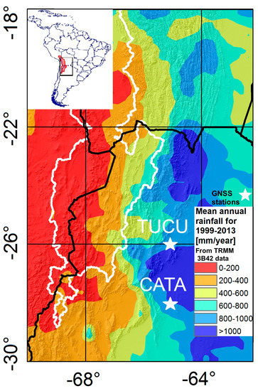
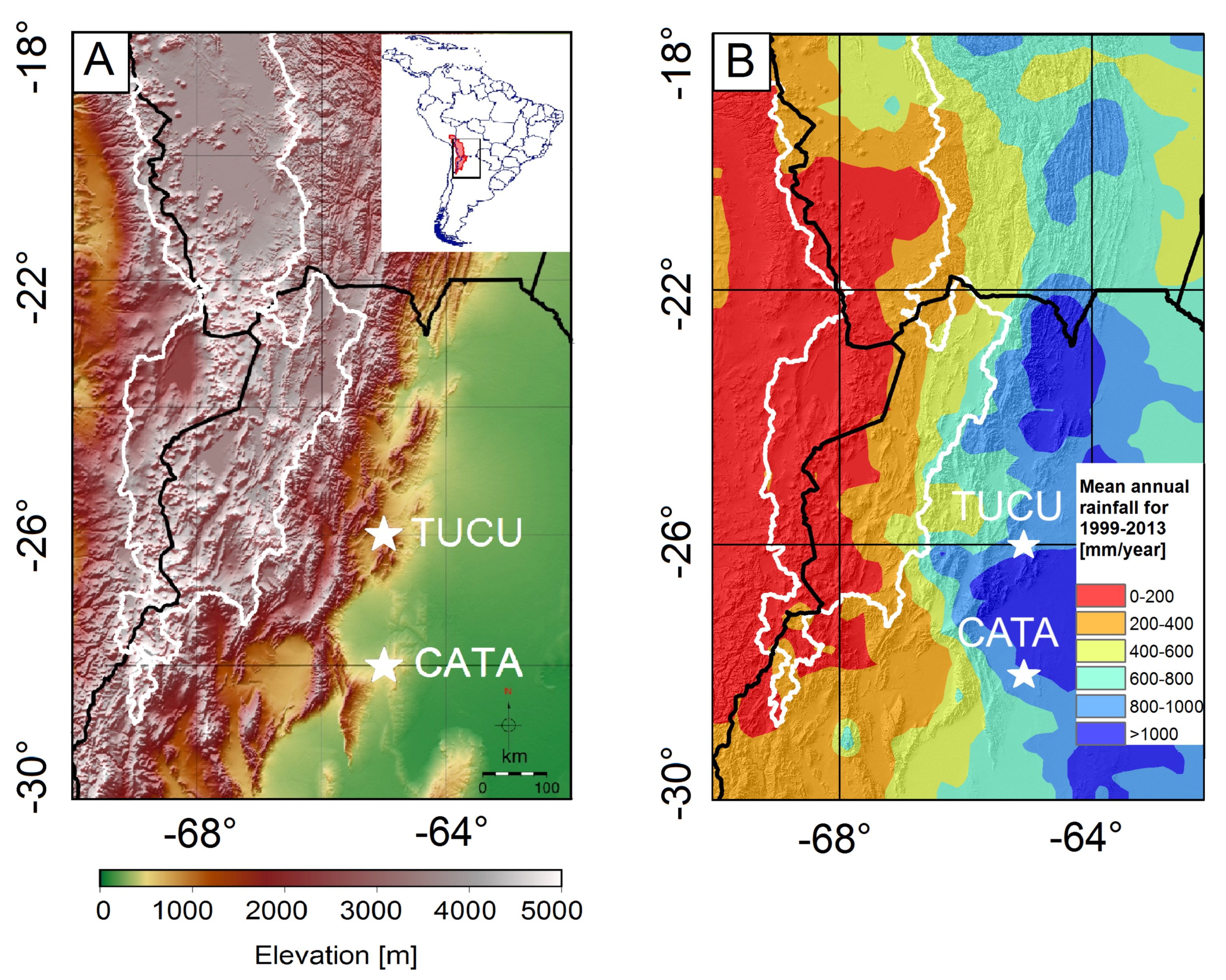
2.1. Data
2.2. GNSS Integrated Water Vapour (IWV) Processing

2.3. Identifying the Effect of GNSS-IWV and CAPE on Extreme Rainfall Formation
3. Results
3.1. Observed Correlation of Rainfall, GNSS-IWV, and CAPE at the GNSS Station Locations
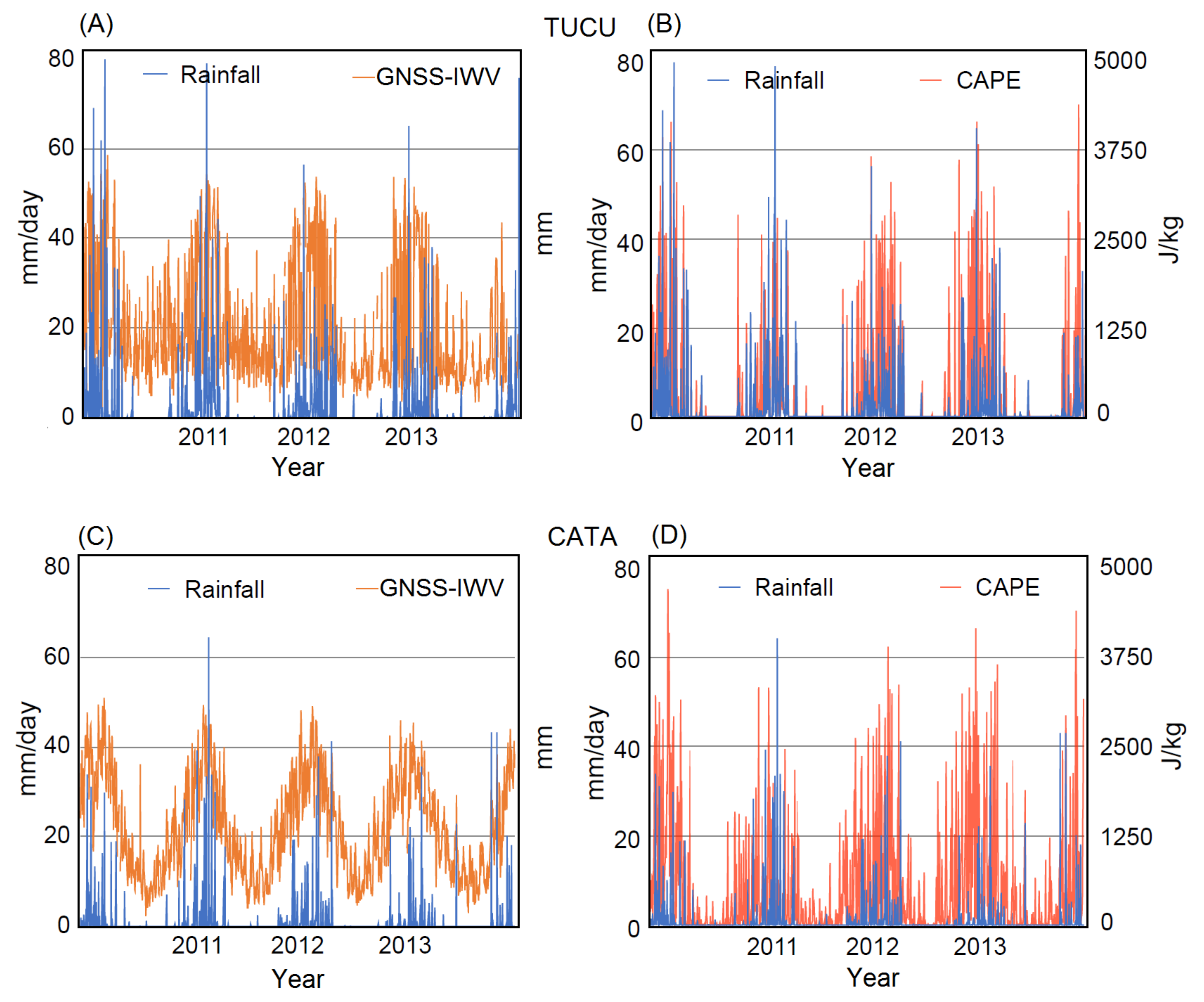
3.1.1. Rainfall, GNSS-IWV, and CAPE Characteristics at the GNSS-IWV Stations
3.1.2. Correlating Seasonal Pattern of GNSS-IWV and CAPE with Rainfall
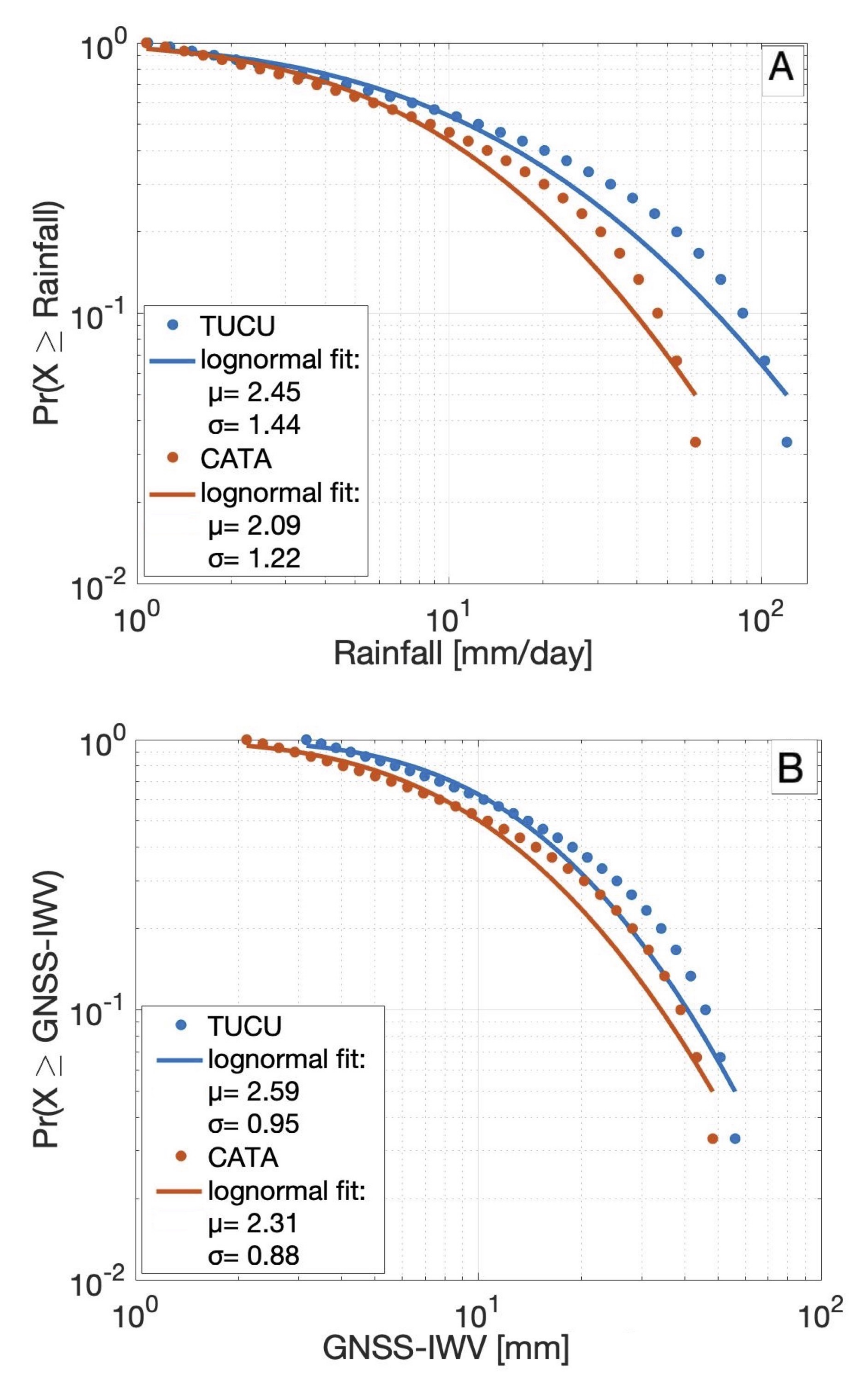
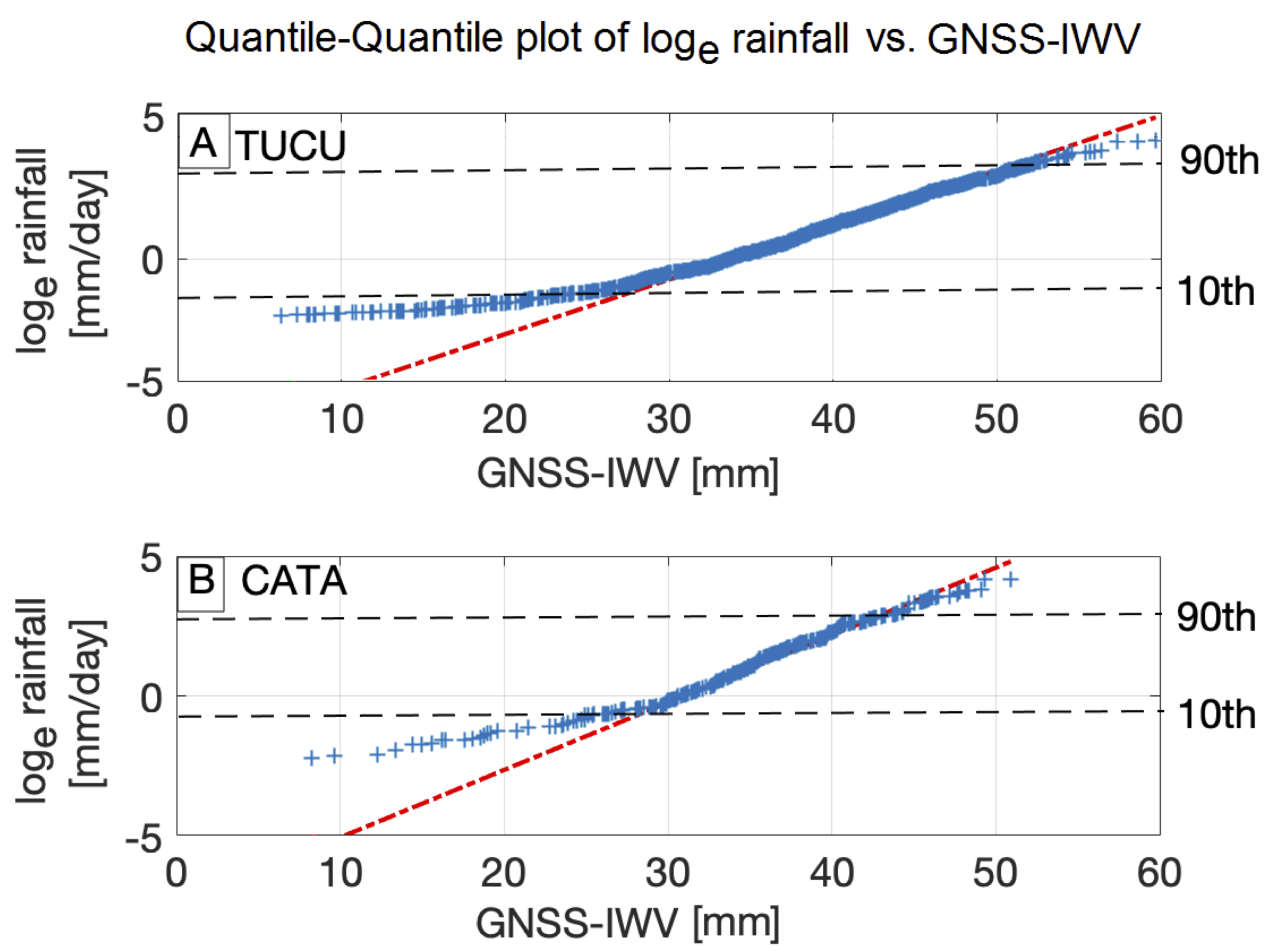
3.1.3. Relation between Rainfall and GNSS-IWV
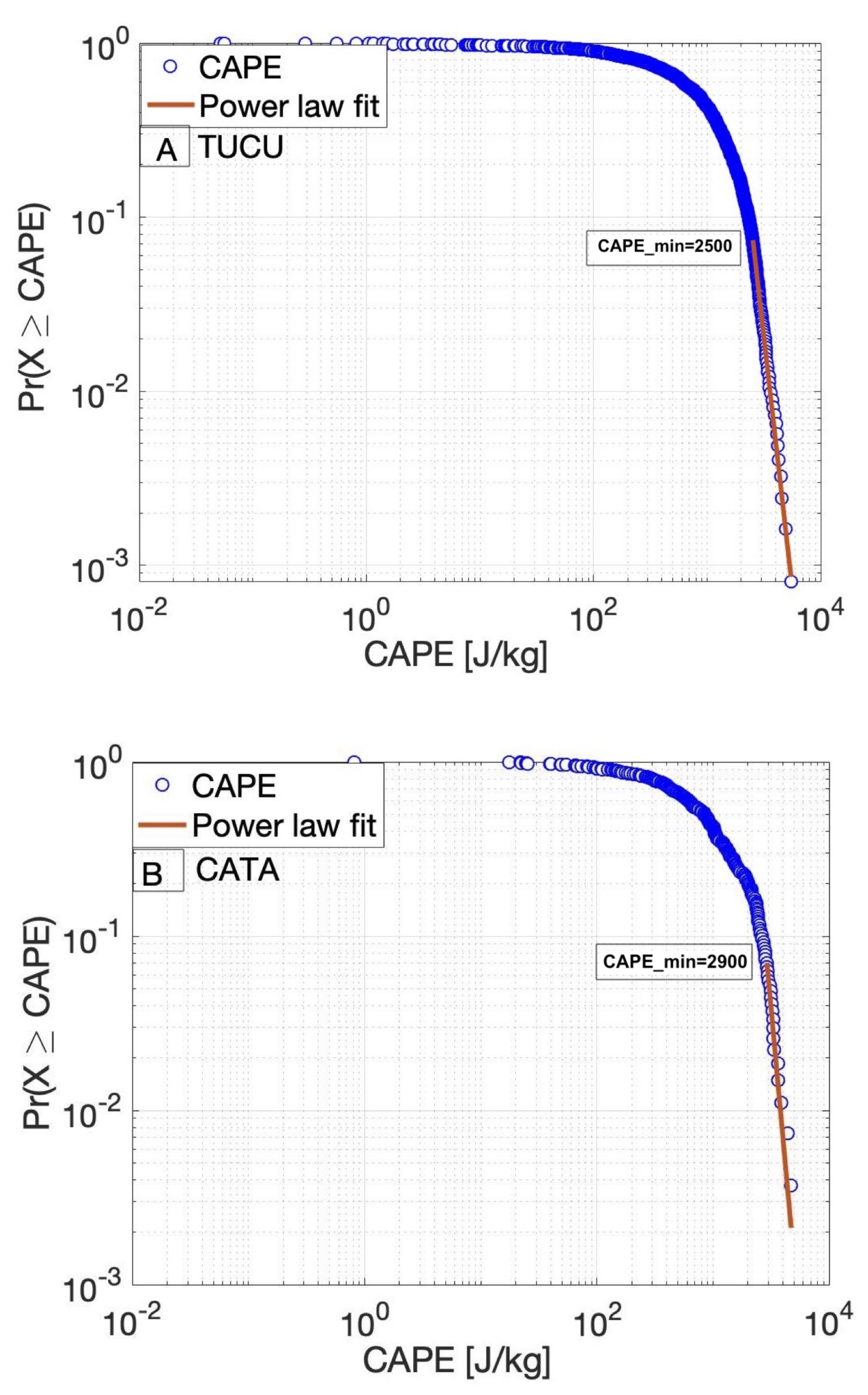
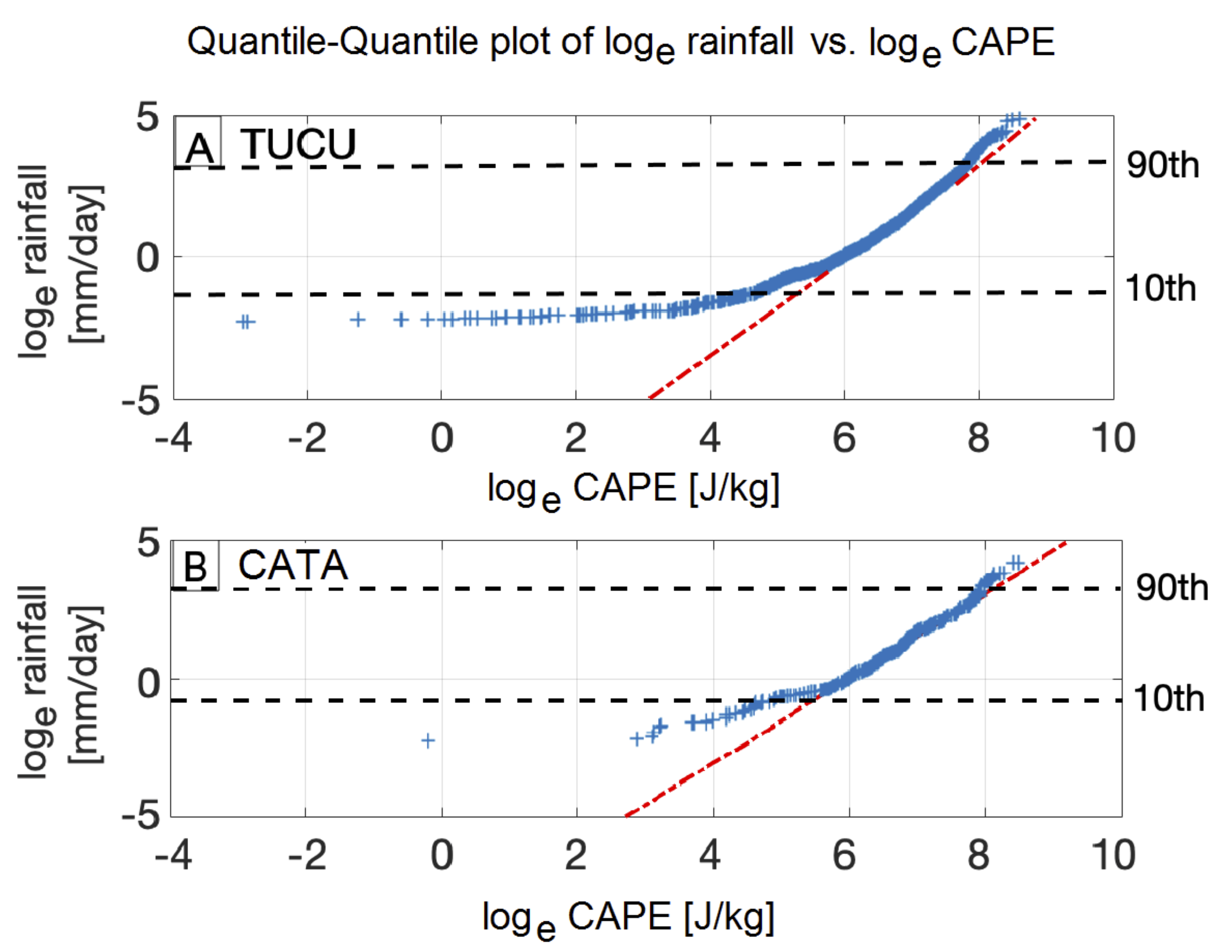
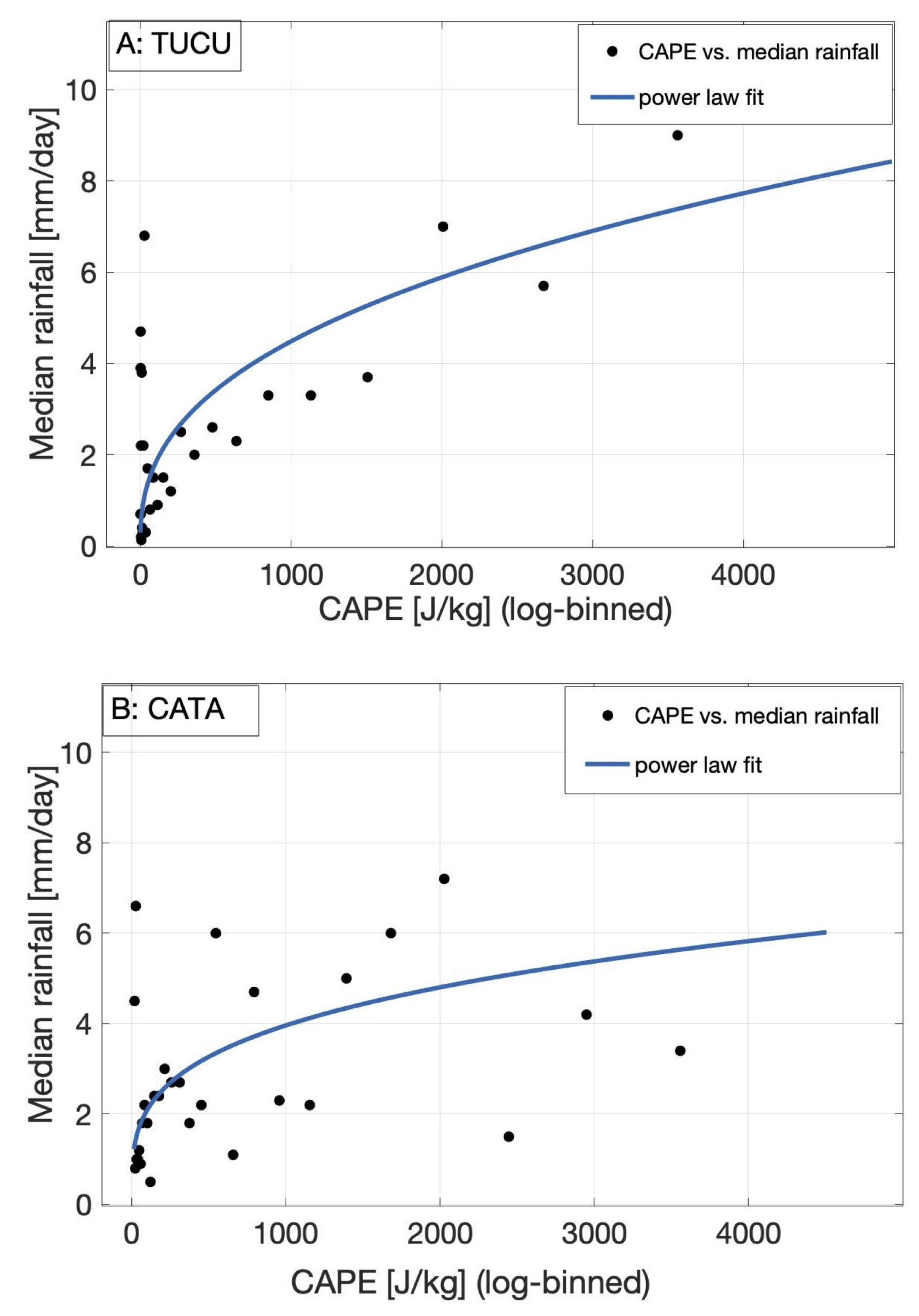
3.1.4. Relation between Rainfall and CAPE
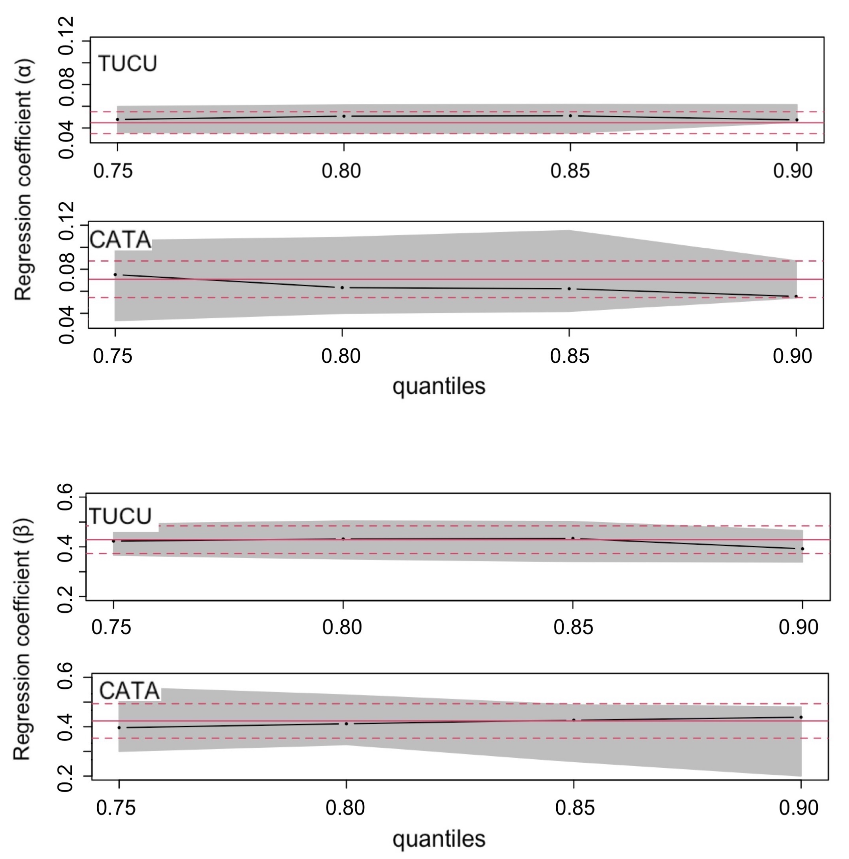
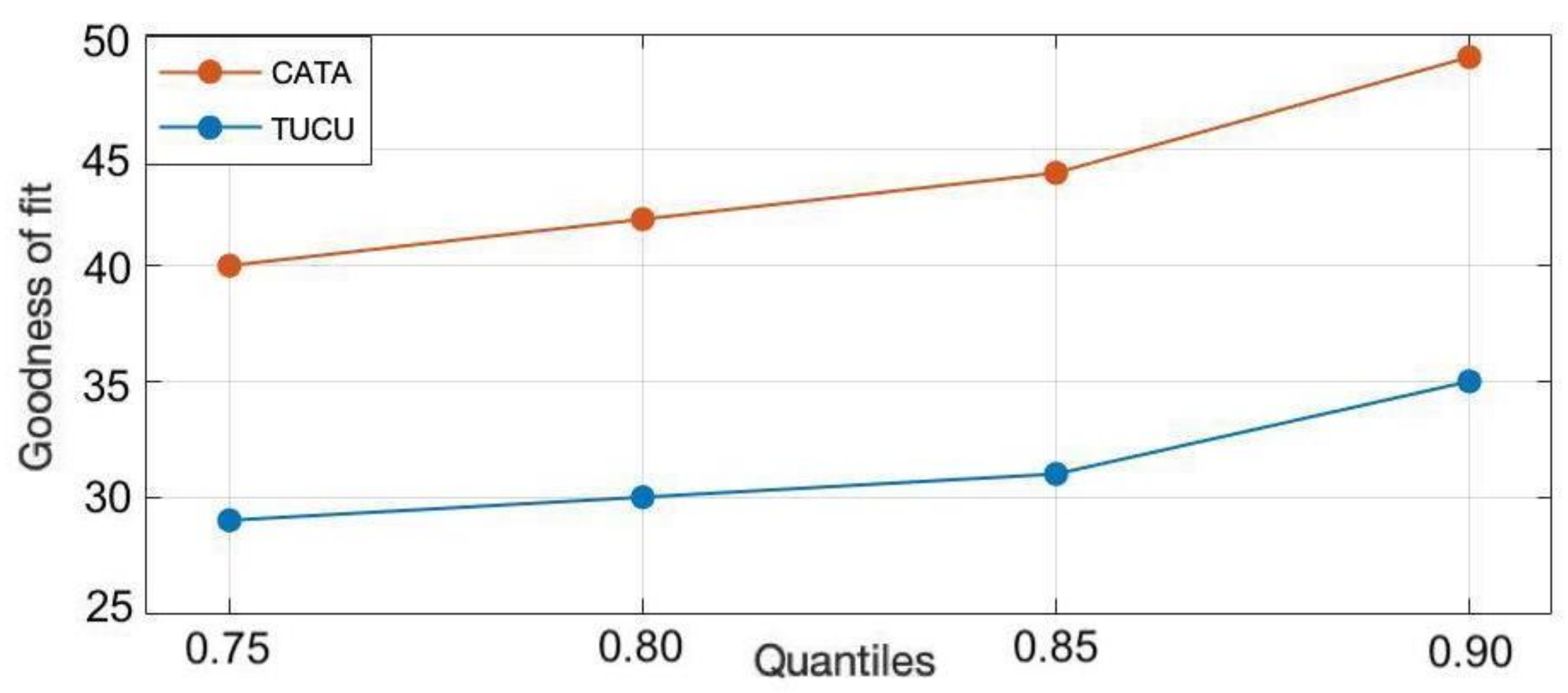
3.1.5. Relation between Rainfall, CAPE, and GNSS-IWV Based on Quantile Regression
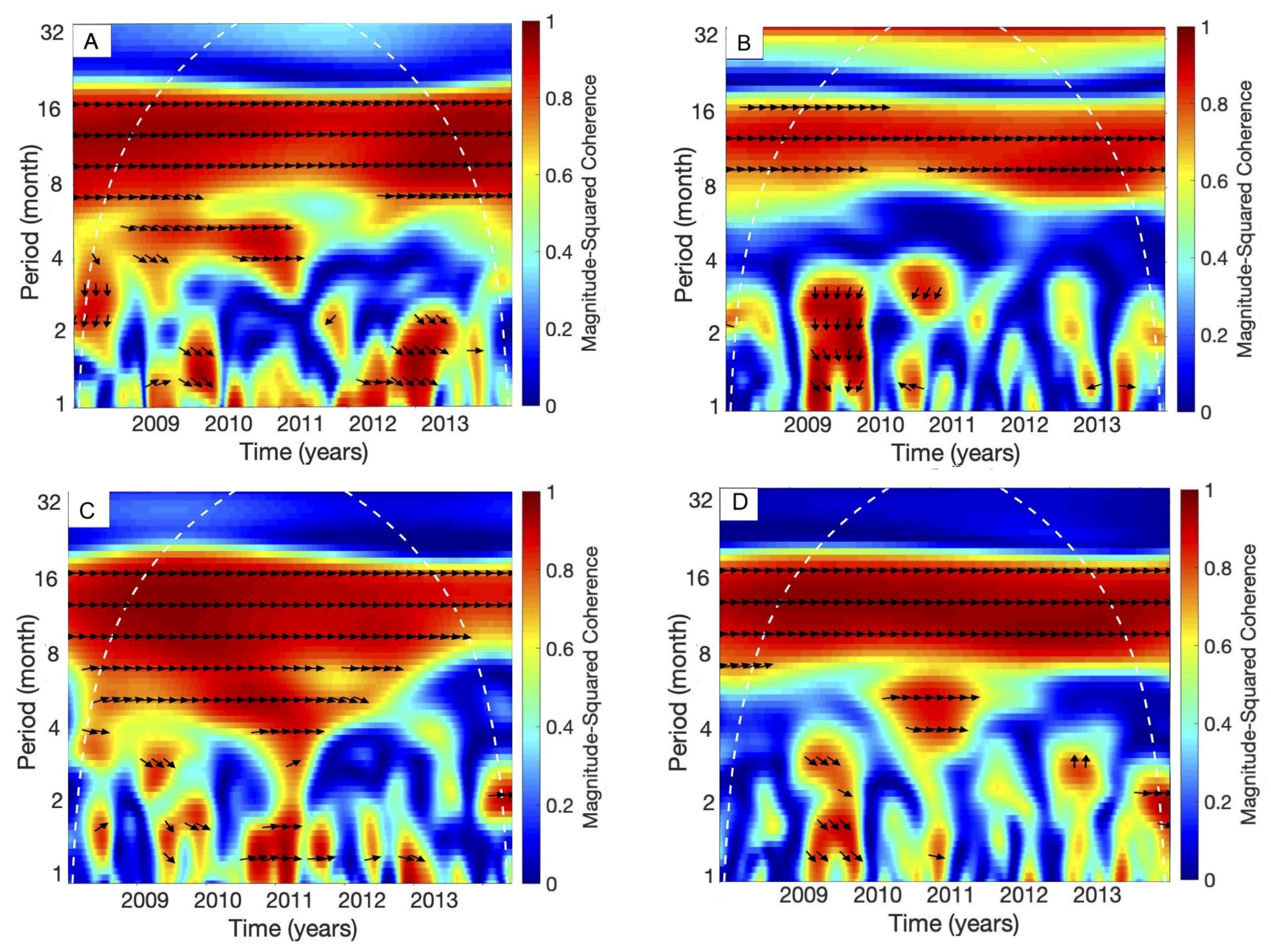
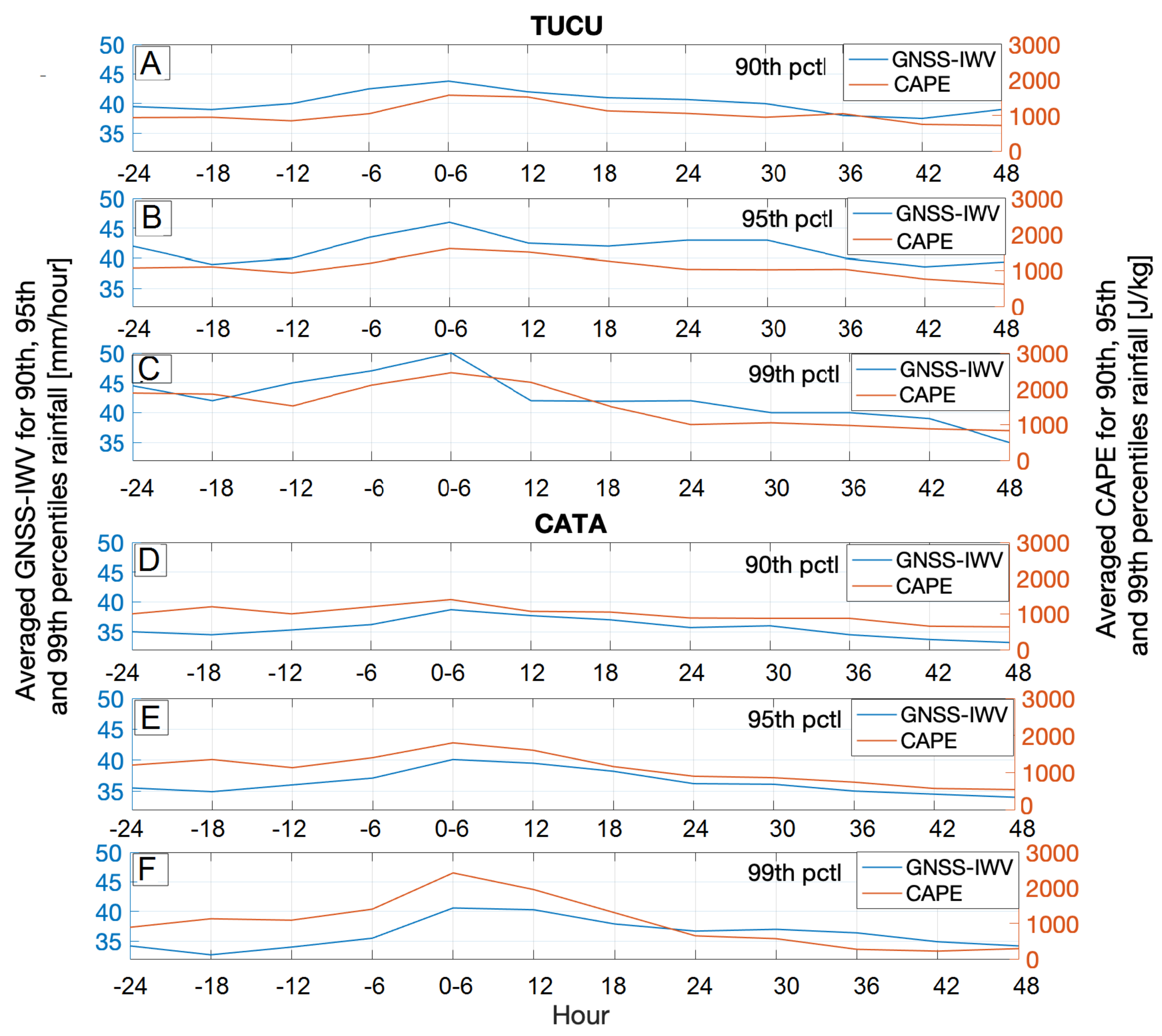
3.2. Temporal Relation between Extreme Rainfall and Both GNSS-IWV and CAPE at the 6-H Time Scale
4. Discussion
5. Conclusions
Author Contributions
Funding
Institutional Review Board Statement
Informed Consent Statement
Data Availability Statement
Acknowledgments
Conflicts of Interest
References
- Castino, F.; Bookhagen, B.; Strecker, M.R. Rainfall variability and trends of the past six decades (1950–2014) in the subtropical NW Argentine Andes. Clim. Dyn. 2017, 48, 1049–1067. [Google Scholar] [CrossRef]
- Boers, N.; Bookhagen, B.; Barbosa, H.M.J.; Marwan, N.; Kurths, J.; Marengo, J.A. Prediction of extreme floods in the eastern Central Andes based on a complex networks approach. Nat. Commun. 2014, 5, 1–7. [Google Scholar] [CrossRef]
- De la Torre, A.; Pessano, H.; Hierro, R.; Santos, J.R.; Llamedo, P.; Alexander, P. The influence of topography on vertical velocity of air in relation to severe storms near the Southern Andes Mountains. Atmos. Res. 2015, 156, 91–101. [Google Scholar] [CrossRef] [Green Version]
- Ramezani Ziarani, M.; Bookhagen, B.; Schmidt, T.; Wickert, J.; de la Torre, A.; Hierro, R. Using Convective Available Potential Energy (CAPE) and Dew-Point Temperature to Characterize Rainfall-Extreme Events in the South-Central Andes. Atmosphere 2019, 10, 379. [Google Scholar] [CrossRef] [Green Version]
- Castino, F.; Bookhagen, B.; de la Torre, A. Atmospheric dynamics of extreme discharge events from 1979 to 2016 in the southern Central Andes. Clim. Dyn. 2020, 55, 3485–3505. [Google Scholar] [CrossRef]
- Castino, F.; Bookhagen, B.; Strecker, M.R. River-discharge dynamics in the Southern Central Andes and the 1976–77 global climate shift. Geophys. Res. Lett. 2016, 43, 679–687. [Google Scholar] [CrossRef]
- Bookhagen, B.; Strecker, M. Spatiotemporal trends in erosion rates across a pronounced rainfall gradient: Examples from the southern Central Andes. Earth Planet. Sci. Lett. 2012, 327, 97–110. [Google Scholar] [CrossRef]
- Rasmussen, K.L.; Houze, R.A. Convective Initiation near the Andes in Subtropical South America. Mon. Weather Rev. 2016, 144, 2351–2374. [Google Scholar] [CrossRef]
- Pingel, P.; Mulch, A.; Alonso, R.N.; Cottle, J.; Hynek, S.A.; Poletti, J.; Rohrmann, A.; Schmitt, A.K.; Stockli, D.F.; Strecker, M.R. Surface uplift and convective rainfall along the southern Central Andes (Angastaco Basin, NW Argentina). Earth Planet. Sci. Lett. 2016, 440, 33–42. [Google Scholar] [CrossRef]
- Rohrmann, A.; Strecker, M.; Bookhagen, B.; Mulch, A.; Sachse, D.; Pingel, H.; Alonso, R.; Schildgen, T.; Montero, C. Can stable isotopes ride out the storms? The role of convection for water isotopes in models, records, and paleoaltimetry studies in the central Andes. Earth Planet. Sci. Lett. 2014, 407, 187–195. [Google Scholar] [CrossRef]
- Bookhagen, B.; Strecker, M. Orographic barriers, high-resolution TRMM rainfall, and relief variations along the eastern Andes. Geophys. Res. Lett. 2008, 35, L06403. [Google Scholar] [CrossRef] [Green Version]
- Rasmussen, K.L.; Houze, R.A. Orogenic Convection in Subtropical South America as Seen by the TRMM Satellite. Mon. Weather Rev. 2011, 139, 2399–2420. [Google Scholar] [CrossRef]
- Priego, E.; Seco, A.; Jones, J.; Porres, M.J. Heavy rain analysis based on GNSS water vapour content in the Spanish Mediterranean area. Met. Apps. 2016, 23, 640–649. [Google Scholar] [CrossRef]
- Adams, D.K.; Fernandes, R.M.; Kursinski, E.R.; Maia, J.M.; Sapucci, L.F.; Machado, L.A.; Vitorello, I.; Monico, J.F.; Holub, K.L.; Gutman, S.I.; et al. A dense GNSS meteorological network for observing deep convection in the Amazon. Atmos. Sci. Lett. 2011, 12, 207–212. [Google Scholar] [CrossRef] [Green Version]
- Berbery, E.H.; Douglas, M.; Enfield, D.; Garreaud, R.; Grimm, A.; Jones, C.; Kousky, V.E.; Lawford, R.; Liebmann, B.; Mechoso, R.; et al. Report of the VAMOS Working Group on the South American Monsoon System (SAMS), Miami, FL, USA, 1998.
- Bevis, M.; Businger, S.; Herring, T.A.; Rocken, C.; Anthes, R.A.; Ware, R.H. GPS meteorology: Remote Sensing of Atmospheric Water Vapour Using the Global Positioning System. J. Geophys. Res. 1992, 97, 15787–15801. [Google Scholar] [CrossRef]
- Bevis, M.; Businger, S.; Chiswell, S.; Herring, T.A.; Anthes, R.A.; Rocken, C.; Ware, R.H. GPS Meteorology: Mapping Zenith Wet Delays onto Precipitable Water. J. Appl. Meteor. 1994, 33, 379–386. [Google Scholar] [CrossRef]
- Duan, J.; Bevis, M.; Fang, P.; Bock, Y.; Chiswell, S.; Businger, S.; Rocken, C.; Solheim, F.; van Hove, T.; Ware, R.; et al. GPS Meteorology: Direct Estimation of the Absolute Value of Precipitable Water. J. Appl. Meteor. 1996, 35, 830–838. [Google Scholar] [CrossRef] [Green Version]
- Chen, B.; Dai, W.; Liu, Z.; Wu, L.; Kuang, C.; Ao, M. Constructing a precipitable water vapour map from regional GNSS network observations without collocated meteorological data for weather forecasting. Atmos. Meas. Tech. 2018, 11, 5153–5166. [Google Scholar] [CrossRef] [Green Version]
- Guerova, G.; Jones, J.; Douša, J.; Dick, G.; Haan, S.D.; Pottiaux, E.; Bock, O.; Pacione, R.; Elgered, G.; Vedel, H.; et al. Review of the state of the art and future prospects of the ground-based GNSS meteorology in Europe. Atmos. Meas. Tech. 2016, 9, 5385–5406. [Google Scholar] [CrossRef] [Green Version]
- Brenot, H.; Neméghaire, J.; Delobbe, L.; Clerbaux, N.; De Meutter, P.; Deckmyn, A.; Delcloo, A.; Frappez, L.; Van Roozendael, M. Preliminary signs of the initiation of deep convection by GNSS. Atmos. Chem. Phys. 2013, 13, 5425–5449. [Google Scholar] [CrossRef] [Green Version]
- Barindelli, S.; Realini, E.; Venuti, G.; Fermi, A.; Gatti, A. Detection of water vapour time variations associated with heavy rain in northern Italy by geodetic and low-cost GNSS receivers. Earth Planets Space 2018, 70, 28. [Google Scholar] [CrossRef] [Green Version]
- Benevides, P.; Catalao, J.; Miranda, P.M.A. On the inclusion of GPS precipitable water vapour in the nowcasting of rainfall. Nat. Hazards Earth Syst. Sci. 2015, 15, 2605–2616. [Google Scholar] [CrossRef] [Green Version]
- Benevides, P.; Catalao, J.; Nico, G. Neural Network Approach to Forecast Hourly Intense Rainfall Using GNSS Precipitable Water vapour and Meteorological Sensors. Remote Sens. 2019, 11, 966. [Google Scholar] [CrossRef] [Green Version]
- Calori, A.; Santos, J.R.; Blanco, B.; Pessano, H.; Llamedo, P.; Alexander, P.; de la Torre, A. Ground-based GNSS network and integrated water vapour mapping during the development of severe storms at the Cuyo region (Argentina). Atmos. Res. 2016, 176, 267–275. [Google Scholar] [CrossRef]
- Lepore, C.; Veneziano, D.; Molini, A. Temperature and CAPE dependence of rainfall extremes in the eastern United States. J. Geophys. Res. 2015, 42, 74–83. [Google Scholar] [CrossRef]
- North, G.R.; Erukhimova, T.L. (Eds.) Atmospheric Thermodynamics; Cambridge Univ. Press: New York, NY, USA, 2009. [Google Scholar]
- Mesgana, S.G.; Thian, Y.G. Trends in Convective Available Potential Energy (CAPE) and Extreme Precipitation Indices over the United States and Southern Canada for summer of 1979–2013. Civ. Eng. Res. J. 2017, 1, 555556. [Google Scholar] [CrossRef] [Green Version]
- Murugavel, P.; Pawar, S.D.; Gopalakrishnan, V. Trends of Convective Available Potential Energy over the Indian region and its effect on rainfall. Int. J. Climatol. 2012, 32, 1362–1372. [Google Scholar] [CrossRef]
- Dee, D.P.; Uppala, S.M.; Simmons, A.J.; Berrisford, P.; Poli, P.; Kobayashi, S.; Andrae, U.; Balmaseda, M.A.; Balsamo, G.; Bauer, P.; et al. The ERA-Interim reanalysis: Configuration and performance of the data assimilation system. Q. J. R. Meteorol. Soc. 2011, 137, 553–597. [Google Scholar] [CrossRef]
- Available online: https://apps.ecmwf.int/datasets/data/interim-full-daily/levtype=sfc/ (accessed on 12 June 2018).
- Ye, B.; Del Genio, A.D.; Lo, K.K.-W. CAPE Variations in the Current Climate and in a Climate Change. J. Clim. 1998, 11, 1997–2015. [Google Scholar] [CrossRef]
- ECMWF. IFS Documentation CY31R1—Part IV: Physical Processes; ECMWF: Reading, UK, 2007; Volume 4. [Google Scholar] [CrossRef]
- Piñón, D.A.; Gómez, D.D.; Smalley, R.; Cimbaro, S.R.; Lauría, E.A.; Bevis, M.G. The History, State, and Future of the Argentine Continuous Satellite Monitoring Network and Its Contributions to Geodesy in Latin America. Seism. Res. Lett. 2018, 89, 475–482. [Google Scholar] [CrossRef] [Green Version]
- Kummerow, C.; Barnes, W.; Kozu, T.; Shiue, J.; Simpson, J. The Tropical Rainfall Measuring Mission (TRMM) Sensor Package. J. Atmos. Ocean. Technol. 1998, 15, 809–817. [Google Scholar] [CrossRef]
- Huffman, G.J.; Bolvin, D.T.; Nelkin, E.J.; Wolff, D.B.; Adler, R.F.; Gu, G.; Hong, Y.; Bowman, K.P.; Stocker, E.F. The TRMM Multisatellite Precipitation Analysis (TMPA): Quasi-Global, Multiyear, Combined-Sensor Precipitation Estimates at Fine Scales. J. Hydrometeorol. 2007, 8, 38–55. [Google Scholar] [CrossRef]
- Available online: https://disc.gsfc.nasa.gov/datasets/TRMM_3B42_Daily_7/summary (accessed on 12 June 2018).
- Carvalho, L.M.V.; Jones, C.; Adolfo, P.; Roberto, Q.; Bookhagen, B.; Liebmann, B. Precipitation Characteristics of the South American Monsoon System Derived from Multiple Datasets. J. Clim. 2012, 25, 4600–4620. [Google Scholar] [CrossRef] [Green Version]
- Boers, N.; Bookhagen, B.; Marengo, J.; Marwan, N.; von Storch, J.; Kurths, J. Extreme Rainfall of the South American Monsoon System: A Dataset Comparison Using Complex Networks. J. Clim. 2015, 28, 1031–1056. [Google Scholar] [CrossRef]
- Gendt, G.; Deng, Z.; Ge, M.; Nischan, T.; Uhlemann, M.; Beeskow, G.; Brandt, A.; Bradke, M. GFZ Analysis Center of IGS—Annual Report for 2013; University of Bern: Potsdam, Germany, 2013; pp. 1–10. [Google Scholar]
- Boehm, J.; Schuh, H. Vienna mapping functions in VLBI analyses. Geophys. Res. Lett. 2004, 31, L01603. [Google Scholar] [CrossRef]
- Deng, Z.; Gendt, G.; Schöne, T. Status of the IGS-TIGA Tide Gauge Data Reprocessing at GFZ. In IAG 150 Years; International Association of Geodesy Symposia; Rizos, C., Willis, P., Eds.; Springer: Berlin/Heidelberg, Germany, 2015; Volume 143, pp. 33–40. [Google Scholar] [CrossRef]
- Gendt, G.; Dick, G.; Reigber, V.; Tomassini, M.; Liu, Y.; Ramatschi, M. Near Real Time GPS Water Vapor Monitoring for Numerical Weather Prediction in Germany. J. Meteorol. Soc. Jpn. Ser. II 2004, 82, 361–370. [Google Scholar] [CrossRef] [Green Version]
- Heise, S.; Dick, G.; Gendt, G.; Schmidt, T.; Wickert, J. Integrated water vapour from IGS ground-based GPS observations: Initial results from a global 5-min data set. Ann. Geophys. 2009, 27, 2851–2859. [Google Scholar] [CrossRef] [Green Version]
- Available online: https://www.gebco.net/data_and_products/gridded_bathymetry_data/version_20141103 (accessed on 10 October 2019).
- Romatschke, U.; Houze, R.A. Extreme Summer Convection in South America. J. Clim. 2010, 23, 3761–3791. [Google Scholar] [CrossRef]
- Koenker, R.; Machado, J. Goodness of fit and related inference processes for quantile regression. J. Am. Stat. Assoc. 1999, 94, 1296–1310. [Google Scholar] [CrossRef]
- Foster, J.; Bevis, M.; Raymond, W. Precipitable water and the lognormal distribution. Geophys. Res. 2006, 111, 2851–2859. [Google Scholar] [CrossRef] [Green Version]
- Springer. The Concise Encyclopedia of Statistics, Lognormal Distribution; Springer: New York, NY, USA, 2008; pp. 321–322. [Google Scholar] [CrossRef]
- Clauset, A.; Shalizi, C.R.; Newman, M.E.J. Power-Law Distributions in Empirical Data. SIAM Rev. 2009, 51, 661–703. [Google Scholar] [CrossRef] [Green Version]
- Sim, I.; Lee, O.; Kim, S. Sensitivity Analysis of Extreme Daily Rainfall Depth in Summer Season on Surface Air Temperature and Dew-Point Temperature. Water 2019, 11, 771. [Google Scholar] [CrossRef] [Green Version]
- Passow, C.; Donner, R.V. A Rigorous Statistical Assessment of Recent Trends in Intensity of Heavy Precipitation Over Germany. Front. Environ. Sci. Eng. 2019, 7, 143. [Google Scholar] [CrossRef]
- Wasko, C.; Sharma, A. Quantile regression for investigating scaling of extreme precipitation with temperature. Water Resour. Res. 2014, 50, 3608–3614. [Google Scholar] [CrossRef]
- Malik, N.; Bookhagen, B.; Mucha, P.J. Spatiotemporal patterns and trends of Indian monsoonal rainfall extremes. Geophys. Res. Lett. 2016, 43, 1710–1717. [Google Scholar] [CrossRef] [Green Version]
- Available online: https://www.ign.gob.ar (accessed on 10 June 2019).


| Model (TUCU) | RMSE | R-Squared |
|---|---|---|
| exponential | 1.3 | 0.17 |
| power | 10 | 0.13 |
| gaussian | 9 | 0.07 |
| polynomial | 11 | 0.09 |
| Model (CATA) | RMSE | R-Squared |
| exponential | 1.56 | 0.15 |
| power | 11 | 0.10 |
| gaussian | 10 | 0.08 |
| polynomial | 11 | 0.09 |
Publisher’s Note: MDPI stays neutral with regard to jurisdictional claims in published maps and institutional affiliations. |
© 2021 by the authors. Licensee MDPI, Basel, Switzerland. This article is an open access article distributed under the terms and conditions of the Creative Commons Attribution (CC BY) license (https://creativecommons.org/licenses/by/4.0/).
Share and Cite
Ramezani Ziarani, M.; Bookhagen, B.; Schmidt, T.; Wickert, J.; de la Torre, A.; Deng, Z.; Calori, A. A Model for the Relationship between Rainfall, GNSS-Derived Integrated Water Vapour, and CAPE in the Eastern Central Andes. Remote Sens. 2021, 13, 3788. https://0-doi-org.brum.beds.ac.uk/10.3390/rs13183788
Ramezani Ziarani M, Bookhagen B, Schmidt T, Wickert J, de la Torre A, Deng Z, Calori A. A Model for the Relationship between Rainfall, GNSS-Derived Integrated Water Vapour, and CAPE in the Eastern Central Andes. Remote Sensing. 2021; 13(18):3788. https://0-doi-org.brum.beds.ac.uk/10.3390/rs13183788
Chicago/Turabian StyleRamezani Ziarani, Maryam, Bodo Bookhagen, Torsten Schmidt, Jens Wickert, Alejandro de la Torre, Zhiguo Deng, and Andrea Calori. 2021. "A Model for the Relationship between Rainfall, GNSS-Derived Integrated Water Vapour, and CAPE in the Eastern Central Andes" Remote Sensing 13, no. 18: 3788. https://0-doi-org.brum.beds.ac.uk/10.3390/rs13183788