Article

Applying a Hand-Held Laser Scanner to Monitoring Gully Erosion: Workflow and Evaluation

1
CSIRO Land and Water, Douglas, Townsville, QLD 4811, Australia
2
CSIRO Land and Water, Dutton Park, Brisbane, QLD 4102, Australia
3
CSIRO Land and Water, Black Mountain, Canberra, ACT 2601, Australia
4
CSIRO Data61, Pullenvale, Brisbane, QLD 4069, Australia
*
Author to whom correspondence should be addressed.
Remote Sens. 2021, 13(19), 4004; https://0-doi-org.brum.beds.ac.uk/10.3390/rs13194004
Submission received: 3 August 2021 / Revised: 14 September 2021 / Accepted: 28 September 2021 / Published: 6 October 2021
(This article belongs to the Section Remote Sensing in Geology, Geomorphology and Hydrology)

Abstract

:
Detailed understanding of gully erosion processes is essential for monitoring gully remediation and requires fine-scale monitoring. Hand-held laser scanning systems (HLS) enable rapid ground-based data acquisition at centimeter precision and ranges of 10–100 m. This study quantified errors in measuring gully morphology and erosion over a four year period using two models of HLS. Reference datasets were provided by Real-Time-Kinematic (RTK) GPS and a RIEGL Terrestrial Laser Scanner (TLS). The study site was representative of linear gullies that occur extensively on hillslopes throughout Great Barrier Reef catchments, where gully erosion is the dominant source of fine sediment. The RMSE error against RTK survey points varied 0.058–0.097 m over five annual scans. HLS was found to measure annual gully headcut extension within 0.035 m of RTK. HLS was, on average, within 6% of TLS for morphological metrics of depth, area and volume. Volumetric change over a 60 m length of the gully and four years was estimated to within 23% of TLS. Errors could potentially be improved by scanning at times of year with lower ground vegetation cover. HLS provided similar levels of error and was relatively more rapid than TLS and RTK for monitoring gully morphology and change.

Graphical Abstract

1. Introduction

1.1. Purpose and Context of Study
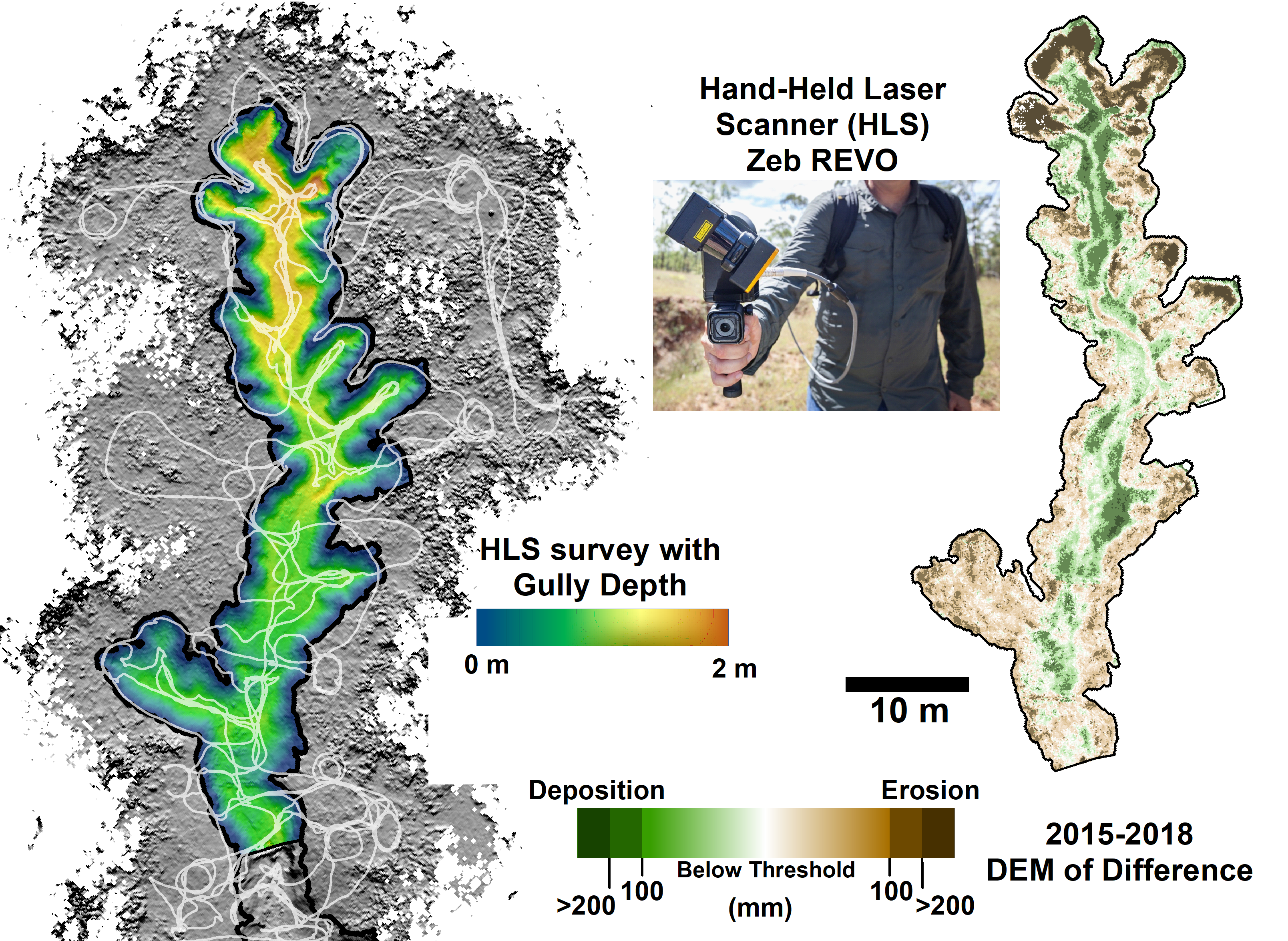
Erosion from gullies is traditionally measured in terms of growth in length, area or volume using airborne LiDAR, Terrestrial Laser Scanning, Real-Time-Kinematic (RTK) GPS and photogrammetry. Each method has unique advantages and limitations in terms of capital and ongoing cost, collection time per unit area, accuracy, repeatability and coverage [1,2,3,4,5,6,7,8,9]. In recent years, improvements in technology have led to the development of hand-held or mobile scanning systems (‘HLS’) designed to enable rapid ground-based survey of complex surfaces [10,11,12].
The health of the Great Barrier Reef (GBR) lagoon is being adversely affected by fine sediment exported from adjacent catchments [1,2]. Tracing studies, erosion mapping and load monitoring have indicated that that the majority of fine sediment exported is derived from eroding subsoil in features such as gullies and streambanks, with gullies contributing approximately 40% of the fine sediment exported from river basins draining into the GBR lagoon [3,4,5]. State and Federal Governments are investing in gully erosion control. Here, as elsewhere, accurately measuring gully morphology and erosion rate is required to inform programs that target and evaluate gully erosion control and ensure the gully treatments are targeted and cost-effective.
Given the successful application of HLS in previous outdoor studies, and their portability, simplicity of use, and potential to capture large complex shapes, there has been interest in applying the technology to gullies. This study had three main aims (1) to develop a workflow for DEM-based products derived from using HLS point clouds at a gully site; (2) to evaluate these gully products against equivalent products from alternative devices, specifically a RIEGL Terrestrial Laser Scanner (TLS) and Real Time Kinematic (RTK) GPS Unit (3) qualitatively compare results to other existing/available/established approaches for evaluating gully change. The results will allow recommendations for appropriate uses for HLS in gully monitoring and improvements to HLS workflow for subsequent gully applications. The testing and evaluation of the HLS was undertaken over a four year period at a gully remediation site in the Burdekin catchment, Queensland, Australia [13].

1.2. Field Site

The gully in this study was within the Weany Creek catchment located on a cattle grazing property approximately 100 km south west of Townsville in Queensland, Australia in the Burdekin River catchment. The Burdekin catchment is the fifth largest in Australia and the highest exporter of fine sediment to the GBR lagoon [14]. The gully site has a dry tropical climate with a long-term average annual rainfall of 618 mm (1889–2017; https://www.longpaddock.qld.gov.au/silo/ accessed on 29 September 2021, most of which falls during the summer monsoon season between November and April. Terrain at the site has a median slope of 2.3% consisting of rolling hills dissected by drainage lines, many of which have branching linear gully features 1–3 m in depth. The dominant soil type, locally known as ‘red goldfields soil’, is a Chromosol (http://www.asris.csiro.au/index.html accessed on 29 September 2021) which is weakly dispersive on some areas of lower slopes, and susceptible to gullying [13].
The gully in this study is partly vegetated [13,15] and is typical of the linear hillslope gullies found in the Burdekin catchment. At least 87,000 kms of linear gullies similar to the study site are estimated to occur within the GBR basins [3,4]. The study gully is approximately 100 m long and 5 m wide with a pronounced headcut approximately 2 m deep with an overhang and side walls typically greater than 50% slope for 50–60 m downstream of the headcut (Figure 1). In 2010 a livestock exclusion fence and six small check dams, constructed of small logs wired together and staked to the gully floor were installed to promote channel deposition and vegetation cover as part of on efforts. The vegetation is typical of the region with open forest forming a discontinuous 7–12 m high canopy dominated by tree species of Ironbark (Eucalyptus crebra) and Bloodwood (Corymbia erythrophloia). Understory consists of grasses, predominantly Indian Couch (Bothriochloa pertusa up to ~30–50 cm high), blackcurrant bushes (Carissa ovata) and woody legumes (Stylosanthes spp.) approximately 1 m tall by 1 m wide. Grasses and shrubs grow on the hillslopes up to the gully edges and in some sections on the more gently sloping gully wall, partly obscuring the bare soil. Leaves, bark and woody debris also partially cover the ground. Pockets of low-lying shrubs and occasional fallen trees and branches occur within the gully. Although cattle were excluded from the gully and adjacent hillslope the vegetation understory still fluctuated annually, growing during the wetter months (December to March), and then drying out or senescing over the course of each dry season.
Capture dates for HLS, TLS and RTK vary within the same year but were treated as equivalent due to the negligible amount of rain and erosion over the intervening dry season period (Table 1). For example, in 2015 there was only 12 mm of rain between 12 April and 4 November and no runoff.

2. Materials and Methods

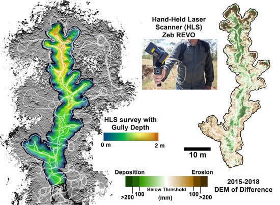
2.1. Hand-Held Laser Scanners (HLS)

An HLS uses an inertial measurement unit or IMU (an accelerometer) to track the movement of a scanning head and. bypasses the need to maintain a stable platform or precise location during scanning. An HLS system called ‘Zebedee’ was developed by CSIRO [16] and commercialized by GeoSLAM as the ‘Zeb1’. The Zeb1 was initially used for mapping underground mines and indoor built environments [17,18], and was subsequently demonstrated to have application in outdoor environments such as mapping cultural heritage sites [19,20], topographic survey [21] and forestry [22]. The Zeb1 has the scanner head mounted on a spring, allowing the head to swing like an inverted pendulum through more than 90 degrees as the operator moved through the environment. A subsequent ‘Zeb REVO’ version of the scanner, with a rotating scanner head mount, was released by GeoSLAM in 2017 [23]. The Zeb1 and the Zeb REVO scanners consisted of four main components, a Hokuyo UTM-30LX-F [24] laser scanner head attached to a handle containing a 3DM-GX2 MEMS IMU [25], a data-logger/control module and a power supply. As both had similar specifications to each other in terms of power, minimum and maximum range and footprint size, they were treated as equivalent in this study and are referred to collectively as ‘HLS’.
After scanning, raw HLS scanner data were processed using SLAM software to identify and align multiple captures of the same object either within one scan or multiple scans (with partly of full overlap) and build a 3-D point cloud [16]. SLAM processing was carried out using GeoSLAM software purchased with the Zeb REVO scanner or, for Zeb1, using SLAM software by the Zebedee development team. Points returned from behind the scanner where the operator was standing were automatically filtered out. Objects in the point cloud were in local coordinates independent of GPS location, but distances were generally accurate and scans were oriented correctly in the vertical direction (Z axis). A separate trajectory file recorded the location of the scanner head during the scan and could be cross-referenced to the point cloud via a timestamp.
The scanner head for both the Zeb1 and the Zeb REVO rotated at 100Hz, generating 41,600 and 43,200 points per second, respectively. Both utilised a 905 nm wavelength laser and provided a typical maximum range for object detection of 15–20 m. The HLS scanner precision is influenced by both intrinsic scan range noise of 3 cm and the Simultaneous Localization and Mapping (SLAM) technology used to reconstruct objects. SLAM precision is environment-dependent, but developers (pers com) estimated it to be approximately 6 cm. Thus, we anticipated HLS precision of around ±9 cm (0.09 m).

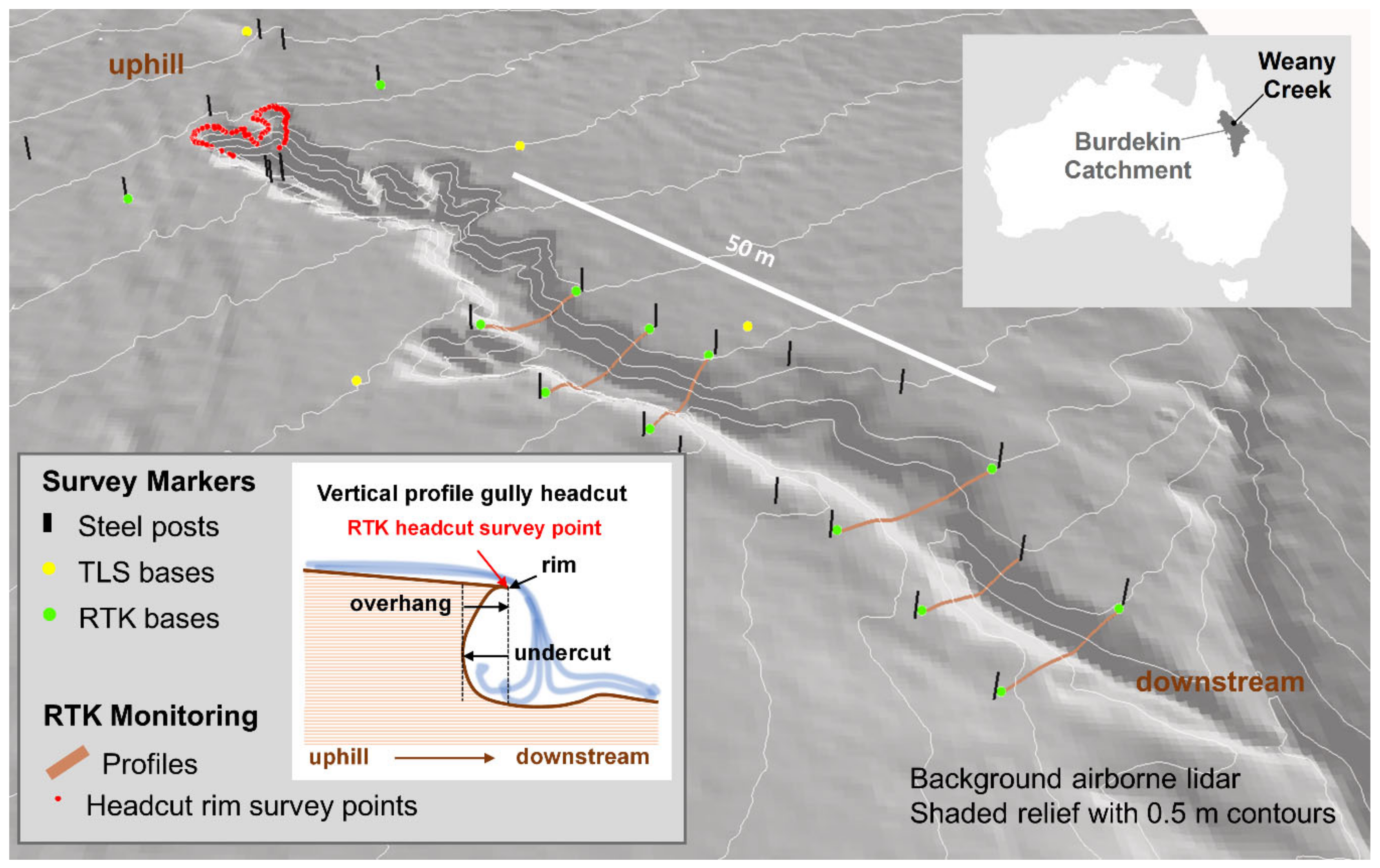
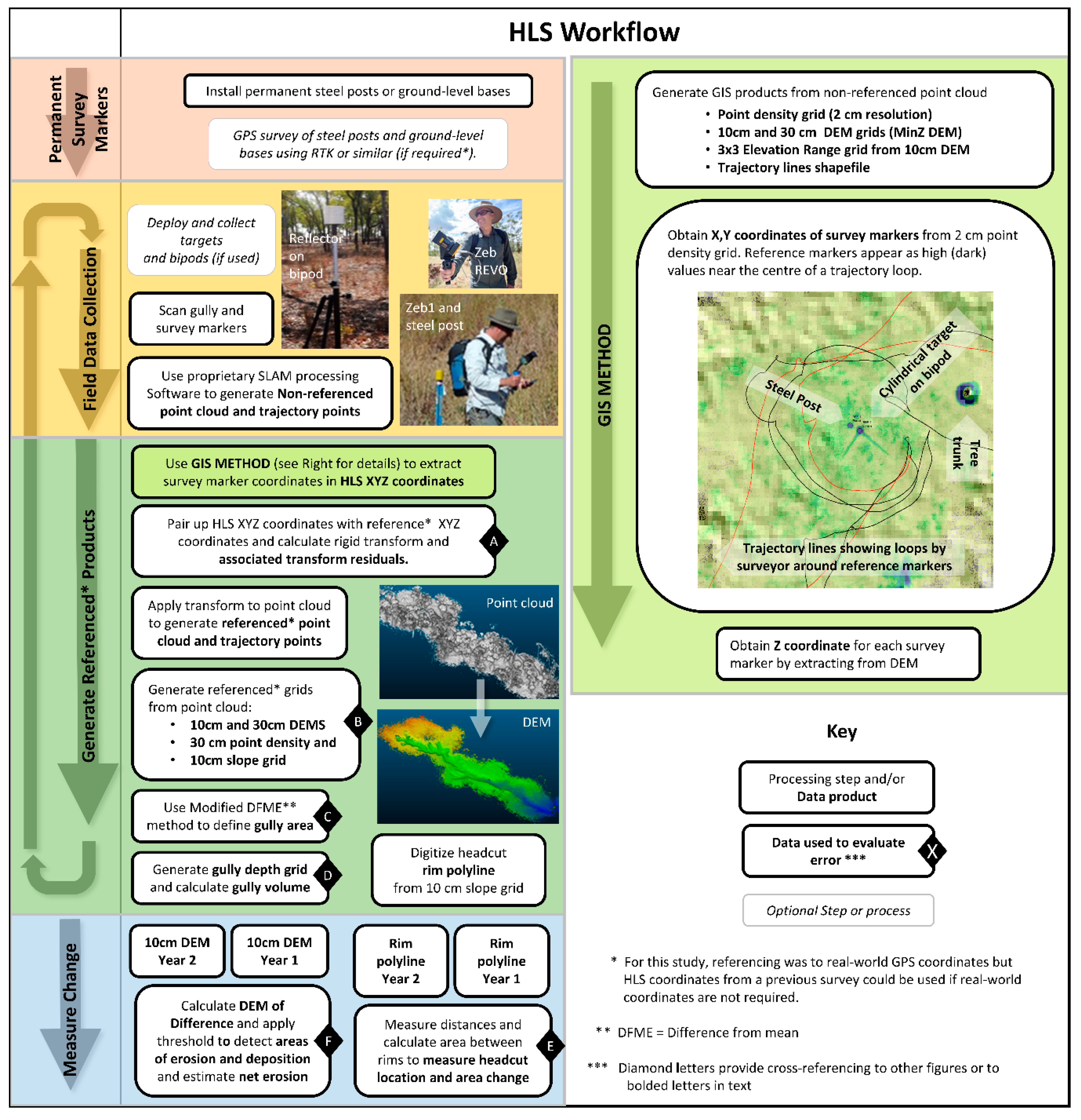
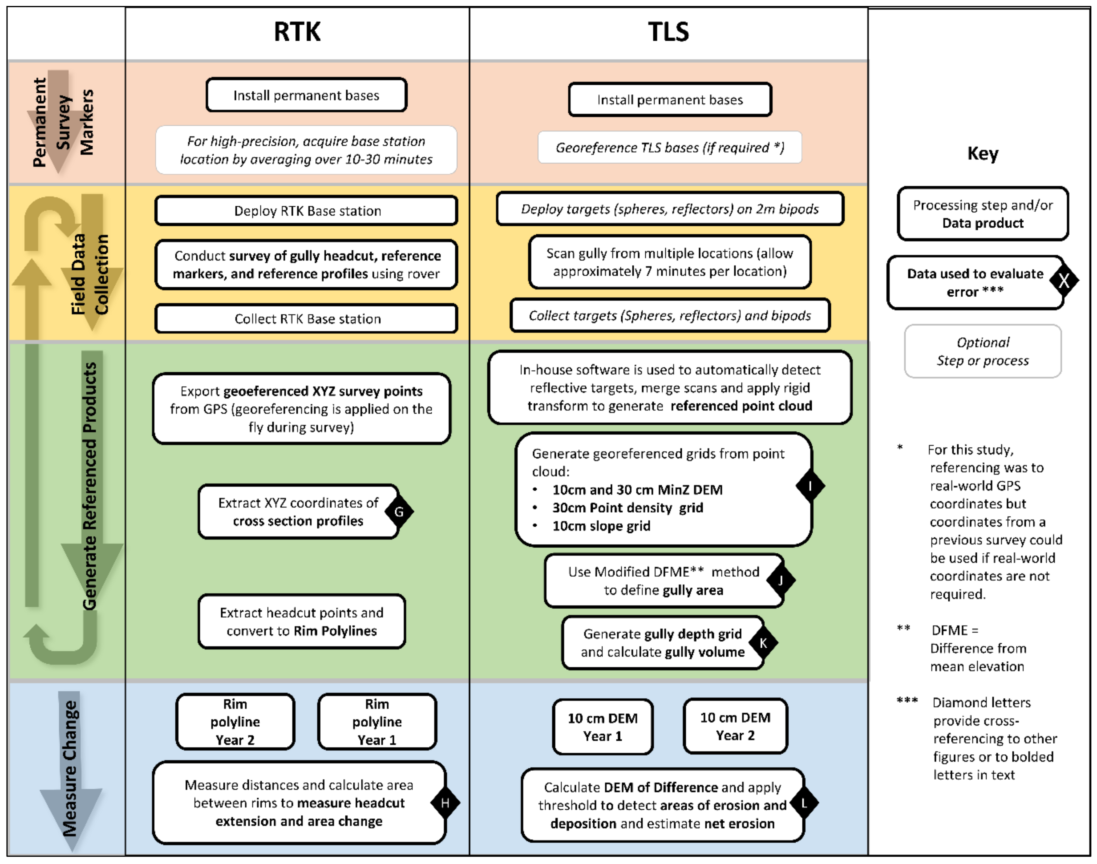
2.2. HLS Workflow for Gully Analysis

Figure 2 shows the HLS gully monitoring workflow developed and refined over the period of this study and is described in more detail below.

2.2.1. Survey Markers and Annual Field Data Collection

Survey markers were used to align HLS scans and validation data. The distribution of these markers around the gully can be seen in Figure 1. TLS bases consisted of a 50 cm steel post driven fully into the ground and surrounded by a concrete collar. RTK concrete bases consisted of a capped metal post embedded in a ground-level pad of concrete. Steel posts were installed using a post driver tool and protruded from the ground to a height of about 1.5 m. A single RTK GPS survey in 2019 captured real-world coordinates (GDA94 MGA55) of the centroid (XY) and ground level (Z) of all survey markers. The tolerance of HRMS and VRMS errors for RTK GPS is ±12 mm and 15 mm, respectively, both are lower than the precision of the HLS. The details of the RTK GPS configuration are discussed in more detail with the validation data. TLS bases and RTK concrete bases were only utilized at time of HLS surveys if temporary targets were deployed on top of these bases. Otherwise HLS surveys relied on the steel posts.
Four HLS surveys were conducted annually during the dry season over a 4-year period (2015–2019). A Zeb1 scanner was used from 2015 to 2017 and a Zeb REVO from 2018 to 2019 (Table 1). HLS scan paths varied from year to year, but all took into account the object detection range (<20 m) and the manufacturers recommendations to scan objects multiple times and to walk in closed loops. Paths aimed to capture the interior surface of the gully, the surrounding hillslope surface and the survey markers at a distance of 1 to 3 m. In general, the scans were initiated upslope from the gully head, circumnavigated the headcut area, then traversed the channel in a downslope direction with break-outs to approach and loop around survey markers. In some years the survey was broken into multiple overlapping scans which could be merged using GeoSLAM’s software. In other years a single scan was used to capture the area with the start and end of the survey providing a closed loop. Scans were limited to 30 min as per the manufacturer’s recommendations.
The output of SLAM processing (settings listed in Table A1 from Appendix A) included a LAS/LAZ format point cloud [26] and a set of trajectory points, indicating the path of the scanner, as an ASCII file. Distances were in units of metres and coordinates were relative to an arbitrary origin near the start of the survey. X and Y axes exhibited an arbitrary orientation in a horizonal plane and the Z axis always showed close orientation with the real-world vertical axis.

2.2.2. Referenced Gridded Products and the GIS Method

Overlaying multiple years of HLS point clouds required firstly obtaining the X, Y, Z coordinates of survey markers in each HLS point cloud to derive a transform. Due to difficulty in the early years getting SLAM or third-party software to automatically detect spheres and cylindrical targets in the point clouds, a GIS Method was developed (Figure 2, right hand side). The GIS Method produced gridded products from the raw HLS point cloud to facilitate extraction of X, Y and Z coordinates corresponding to the base of each survey marker. It had an additional advantage over automatic point cloud detection methods as it could also detect steel posts, which are numerous at this site (Figure 1) required no pre-scan target deployment, and were much easier to install than TLS or concrete bases.
The GIS Method was implemented in ArcGIS and started by automatically generating products from the LAZ point cloud and trajectory files from the SLAM processing. These products included a:
  • 10 cm grid of the minimum Z value within each grid cell (10 cm DEM) as a detailed representation of the ground surface. Minimum point density of 10 points per grid cell is assumed sufficient to detect at least one ground point, although this DEM will contain vegetation artifacts around the periphery (DEM inset in Figure 2) where tall features such as trees may enhance point density but scanner is not reliably detecting ground due to the flat angle of scan.
  • 30 cm grid of the minimum Z value within each grid cell (30 cm DEM) for use where the 10 cm DEM is noisy (due to dense vegetation) around a survey markers and for derivation gully area.
  • Elevation range grid representing the range of 10 cm DEM values in a 3 × 3 grid cell area. This was used as an indicator of reliability of ground detection near survey markers.
  • Point density (count) grid at 2 cm resolution for detection of survey markers
  • Point density (count) grid at 30 cm resolution for determining the limits of reliable data at the edges of the scan.
  • Shaded relief image from the 10 cm DEM for visualization and context.
  • Trajectory polyline (from the trajectory point cloud) showing the path of the scanner.
In the 2 cm resolution point density grid, each survey marker was identifiable as a small cluster of high-density pixels centred near the middle of the trajectory loop (GIS Method screen shot in Figure 2). The centre of this pixel cluster was digitized and labelled with its unique survey marker name. It was also possible to copy a pre-existing set of marker points (e.g., from a previous year’s scan), apply a bulk re-alignment to the new scan and then fine-tune the pre-labelled marker locations in the new scan. Once survey marker points were positioned correctly over the point density grid in the GIS and their XY locations extracted, a Z value was obtained from the 10 cm DEM representing the ground level at the base of the marker. If the elevation range grid indicated a range of Z values greater than 0.1 m within the surrounding pixels, for example due to poor ground detection through vegetation, the 30 cm DEM was used to extract Z instead. The XYZ coordinates generated using this GIS Method were then paired with corresponding GDA94 MGA55 coordinates from the 2019 RTK survey.
Rigid transforms are an industry-standard method for referencing point clouds [27,28] and involve collecting paired coordinates for each survey marker to derive transform matrices (translation and rotation, no scaling) of the non-referenced HLS point cloud to the referenced coordinates. The transform was calculated using an in-house Python script which generated a 4 by 4 transform matrix and a set of residuals (A in Figure 2). Transform residuals recorded the difference between the Reference XYZ location and the transformed XYZ location for each survey marker. If the overall RMSE of the residuals exceeded one DEM pixel (0.1 m), the survey marker with the highest errors was treated as an outlier and removed. The transform matrix was regenerated until an RMSE of less than 0.1 m was achieved. Removing outliers to achieve our target RMSE allowed for appropriate management of the occasional legitimate error (e.g., non-ground in the 10 cm DEM, or incorrect identification of survey marker) and has been used in other remote sensing and scanner studies [8]. The transform was then applied to the HLS point cloud and trajectory points in CloudCompare (Version 2.11) software using ‘Global Shift and Scale’ and ‘Apply Transform’ tools (http://www.cloudcompare.org/ accessed on 6 August 2019).
The referenced point cloud for each year was then used to generate a 10 cm DEM and the other GIS products (B in Figure 2), but this time using the point cloud and trajectory points in the reference coordinate system. A percent slope grid was also derived from the referenced 10 cm and 30 cm DEMs using Spatial Analyst in ArcGIS [29].

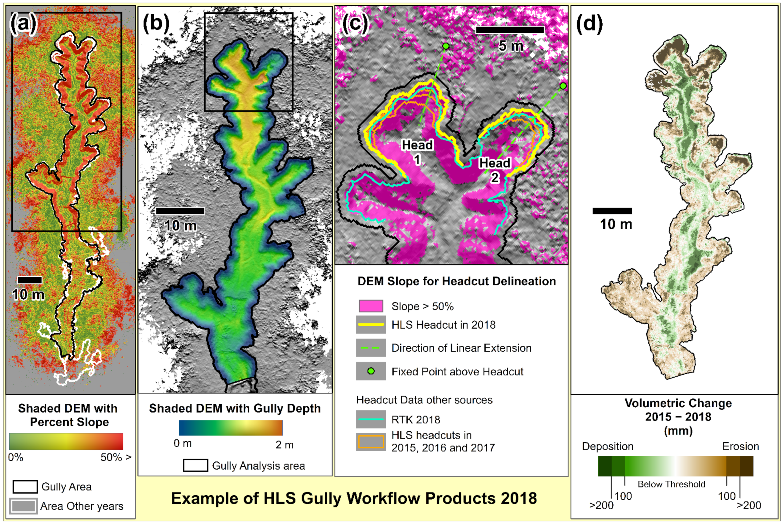
2.2.3. Gully Morphology—Area, Depth and Volume and Headcut

An ArcGIS script was used to automate a Modified Difference from Mean Elevation (DFME) algorithm [30]. DFME differentiates the area inside from the area outside a gully by comparing the elevation of a grid cell with its surroundings, as gullies are lower than their surroundings. The 30 cm DEM, while coarse, had less vegetation influence around the scan margins than the 10 cm DEM, making it more suited to DFME analysis. A mask was applied to the 30 cm DEM, defined by largest contiguous polygon with a 30 cm point density grid value greater than 100, to further reduce vegetation effects at the margins. DFME was then derived from the masked 30 cm DEM using a mean elevation window diameter of 10 m (approximately twice the width of the gully). The preliminary gully area, defined by DFME < 0, underestimated gully area slightly, with the boundary sitting just inside the steepest part of the gully rim. Thus, the area was “grown” to include any 30 cm grid cells where the maximum percent slope within a 30 cm radius was 25% or more. Occasional non-gully “holes” remained in the resulting gully area polygon and were removed manually. Reliable detection of gully area reduced toward the downstream end of the gully due to flattening of gully walls downstream. Thus the final gully area polygon (C in Figure 2) was truncated. Criteria for this truncation could relate to morphology (e.g., distance after which the gully walls no longer exceed 50% slope) or DEM quality (e.g., sparse points creating noise at the downstream limits of survey). However, for this case study, the gully areas for all years were truncated to a length of approximately 60 m from the headcut to match the extent of the TLS validation data.
A gully depth grid (D in Figure 2) was derived from a DEM of Difference (DoD) between a gully “lid” and the 10 cm DEM calculated within the extents of the gully area polygon. This depth grid was used to estimate maximum gully depth and gully volume. The lid was created by constructing a gridded surface from a Triangulated irregular network (TIN) connecting the 30 cm DEM pixels just outside the gully area polygon. Maximum depth was the largest depth grid value in this grid, while volume (in m3) was the sum of all depth grid cell values (in m’s) multiplied by the cell size (in m2).
Headcut retreat can be a useful measure of gully erosion, as headcuts are usually the most active part of the gully. Headcuts often have near-vertical profiles in a Minimum Z DEM and can thus be detected by a rapid increase in slope. The percent slope grid derived from the 10 cm DEM was used to generate a headcut polyline defined by the slope transitioned from <50% to >50% at the upstream apex of the gully and for a distance 3–5 m to either side, depending on gully morphology.

2.2.4. Measuring Change between Years

The most visible area of change in a gully is the headcut. HLS headcut methods in workflow were adapted from previous survey methods used at this gully. Headcut retreat was measured as a single value of linear extension and as an average value based on change in headcut area (E in Figure 2). Linear extension of the headcut between years was determined by measuring the decrease in distance from the digitized headcut rim to a fixed position upstream of the headcut. The average headcut extension between years was calculated as the area between the two rim polylines divided by the length of the outmost (newest) headcut. Changes in the gully below the headcut are usually subtle but may be estimated using volumetric change analysis.
Gully volume estimates from the gully depth grid for individual years were not precise enough for estimation of the volumetric change (net erosion) between years due to slight variations in lid levels between years. However, a DEM of difference (DoD) calculated by cell-by-cell subtraction of one referenced 10 cm DEM from another (F in Figure 2) avoids lid issues and is a standard method of detecting volumetric change [31]. DoDs are essentially maps showing areas of erosion and deposition. Referenced 10 cm DEMs clipped to the latest (2019) gully area polygon were used to derive DoDs. DoDs recognize uncertainty by application of a threshold value below which no change is assumed to have occurred. A single threshold value was used for all DoDs and was based on an estimate of the critical threshold error Ucrit ([31], (1) derived using 10 cm DEMs from duplicate HLS surveys (4 November 2015, Table 1). All DOD values with absolute values greater than the UCrit threshold were identified as erosion (negative DoD) or deposition (positive DoD). Planimetric area (AreaP) and average depth (DepthAvg) are reported separately for erosion (eros) and deposition (dep) ((2) and (3), respectively) and can be used to calculate volumetric change. Volumetric change (VolΔ) calculated using erosion and deposition components (4) is equivalent to the more traditional cell-by-cell method of calculating volumetric change from a DEM of difference (5), but provides more information about the sources of error. For this study, the volume of erosion was reported as a positive value and volume of deposition as a negative value (i.e., the reverse of the DoD height changes).
U C r i t = t σ e 1 2 + σ e 2 2
where Ucrit is the critical threshold error based on a critical student’s t-value set to a 95% confidence interval (t = 1.96) and σe1 = σe2 is the standard deviation of all gully grid cells in the DoD of 10 cm resolution DEMS from duplicate scans.
A r e a P e r o s = c e l l   a r e a w h e r e   D o D < t h r e s h o l d A r e a P d e p = c e l l   a r e a w h e r e   D o D > t h r e s h o l d
D e p t h A v g e r o s = 1 × D o D / A r e a P e r o s w h e r e   D o D < t h r e s h o l d D e p t h A v g d e p = D o D / A r e a P d e p   w h e r e   D o D > t h r e s h o l d  
V o l Δ = V o l Δ e r o s V o l Δ d e p   = A r e a P e r o s × D e p t h A v g e r o s A r e a P d e p × D e p t h A v g d e p
V o l Δ = 1 × D o D × c e l l   a r e a w h e r e   a b s D o D > t h r e s h o l d

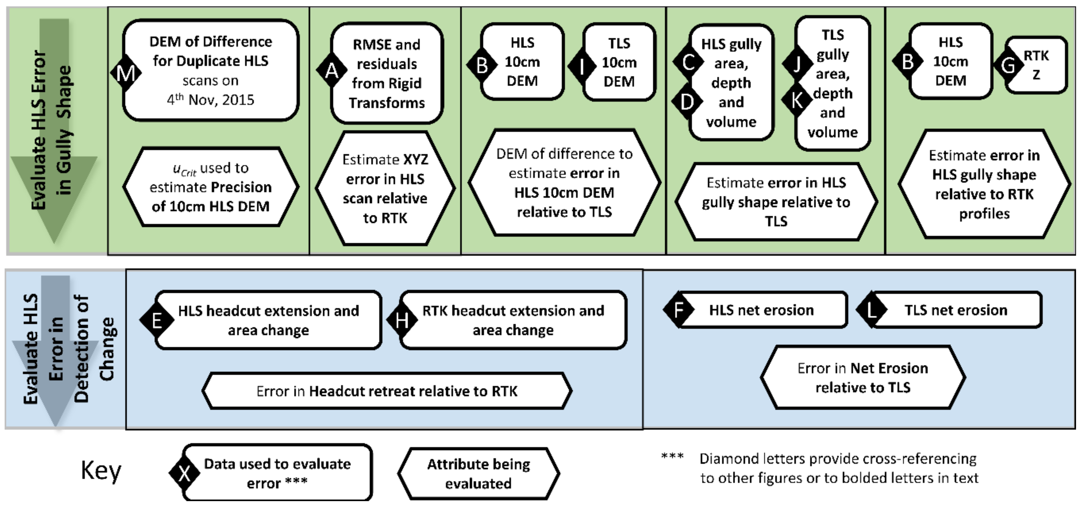
2.3. Evaluation of Error

2.3.1. Validation Data

Validation data were sourced from Real Time Kinematic (RTK) GPS and Terrestrial Laser Scanner (TLS) surveys. It was recognized that these systems have their own precision limits. Thus, for the purposes of this study HLS error should be interpreted as error relative to validation data.
The RTK GPS system used was an Ashtech ProMark 200 with a tolerance of +/−12 mm in the horizontal plane and 15 mm in the vertical. RTK utilizes a base station unit to provide a fixed reference which is used to provide precise locational information to a Rover unit moved around the site on a fixed height (2 m) pole. Annual RTK surveys at the gully captured concrete bases, gully cross-sections, the gully bed long section along the deepest part of the channel, and the changes in location and shape of the headcut rim. Annual RTK survey data consisted of a table of unique IDs, descriptive labels, XYZ coordinates (GDA94 MGA55 eastings and northings and Australian Height Datum elevations, respectively), and additional information relating to precision, which can vary depending on line-of-sight to satellites and base station. This table was imported into the GIS as points with all attributes preserved. Based on comparison between annual surveys of survey markers, the precision of the RTK data averaged ±5 cm in the horizontal and vertical directions.
The TLS instrument used in this study was the RIEGL VZ400 (122,000 points per second with 350 m range). Each survey consisted of several scans, collected by moving the scanner to different locations around the gully, placing it on a tripod and leaving it to scan for approximately 5 min. Prior to scanning, cylindrical reflectors were mounted 2 m above the TLS bases using survey bipods. Additional mobile reflectors were distributed around the site, (see [28]). The RIEGL has an inbuilt fine-scan option which utilizes the reflector signals, internal GPS and digital compass to register scans into the same coordinate system with errors typically <1 cm. For this study, a further rigid transform was applied to precisely match the TLS point cloud to the HLS point cloud using the TLS base coordinates surveyed by RTK in 2019.

2.3.2. Validation Data Workflow

Figure 3 shows the workflow applied to RTK and TLS data to produce validation data. The workflow for HLS shown in Figure 2 was designed to emulate the type of products and measurements already developed for these instruments within the precision limits of the HLS. Where necessary for direct comparison, the same resolution or thresholding was applied to validation data as for HLS.
RTK surveys included cross-sections and polylines generated from rim survey points. For validation of gully morphology, HLS 10 cm DEM Z values were extracted at each RTK cross-section point for the corresponding year and compared to the RTK Z values (G in Figure 3). Poor precision RTK points (“floating” due to satellite or vegetation issues) were excluded from the validation data. Comparison of cross section points is based on the line of best fit between HLS and RTK Z values and an overall RMSE. For validation of HLS headcut retreat rates (E in Figure 2), the RTK rim surveys were converted to polylines (H in Figure 3). RTK headcut linear extension and changes in headcut area are compared to equivalent HLS measurements using a line of best fit and overall RMSE. HLS DEMs cannot represent overhangs, a common feature of gully headcuts (inset in Figure 1) and the RTK rim surveys capture the edge of the overhang. Thus an offset in location of the headcut between RTK and HLS is expected, but validation will consider only the rates of extension of the headcut.
Validation data from TLS included a 10 cm DEM for each year (I in Figure 3) generated at exact cell locations as HLS (B in Figure 2), a gully area polygon (J in Figure 3), and depth and volume estimates (K in Figure 3) using the same method as HLS. In addition, a comparison was made of the DEMs of Difference (DoD) for the HLS 10 cm DEMs and TLS 10 cm DEM to investigate spatial patterns of error in the HLS scans. For validation of net erosion estimates from HLS (F in Figure 2), TLS 10 cm DEMs of difference (L in Figure 3) were generated using the same methods as HLS, including the same pixel locations, gully area (2019 TLS gully area) and threshold of detection.

2.3.3. Error Analysis

Figure 4 shows the HLS errors evaluated in this study. Black diamond letters provide a cross-reference to relevant components of the workflows in Figure 2 or Figure 3. In addition to comparing HLS to the validation RTK and TLS data, residuals from rigid transforms and duplicate HLS surveys provide information about scan distortions and inherent precision of the DEMs, respectively. The Root Mean Square Error RMSE of the transform residuals (A in Figure 2) provides an overall measure of scan error while the spatial patterns of residuals provide clues to the nature of scan distortions contributing to these errors. Ten-centemeter DEMs from duplicate HLS surveys (M in Figure 4) allow the estimation of critical threshold error Ucrit (1).
For detection of change, net erosion was evaluated using two different reference years, 2015 (the start year of the study) and 2019 (the end year of the study), to derive a timeseries of increasing intervals up to the maximum 4 years (2015–2019). This was carried out in recognition that errors in the data for a given reference year had potential to propagate systematically through all measures of change against that year.

3. Results

3.1. Outputs from HLS Workflow

Within the gully and gully rim area, HLS point counts for all years were greater than 10 points within any given 10 cm by 10 cm area (median count was between 110 and 250 points). Given the density of vegetation cover in the gully, such point counts provided confidence that the 10 cm and 30 cm MinZ DEMs derived from the HLS workflow were detecting the ground surface in all but the rarest of instances. Figure 5 shows the outputs from the HLS workflow for 2018. In Figure 5a, the 2018 HLS slope grid is overlain by the DFME-derived HLS gully area polygons in white for all years up to 2018 (i.e., 2015 to 2018 inclusive). In the upstream half of the gully, gully areas show a general progression of the headcut in an upstream direction from 2015 to 2018. In the downstream half, gully area appears more random due to difficulty of DFME detecting flatter gully walls.
Figure 5b shows the gully depth grid used to estimate gully volume. Gully area for the depth grid was limited to 60 m from the headcut to represent the area of overlap with TLS data. Figure 5c shows the headcut rim polylines, where slope transitions from <50% to >50%. The RTK headcut rim survey (for 2018 shown in blue) is consistently offset downstream from HLS for all years by a distance consistent with the undercut of the headcut (0.3–0.5 m, Figure 1). Despite uncertainty due to undercutting, headcut progression is detectable with HLS (orange lines). Areas of erosion and deposition detected by the DEM of difference in Figure 5d show that HLS is detecting realistic patterns of erosion and deposition over the 3-year period from 2015 to 2018, with erosion dominating the headcut area and deposition occurring in channel area.

3.2. HLS Repeatability and Error in Gully Morphology

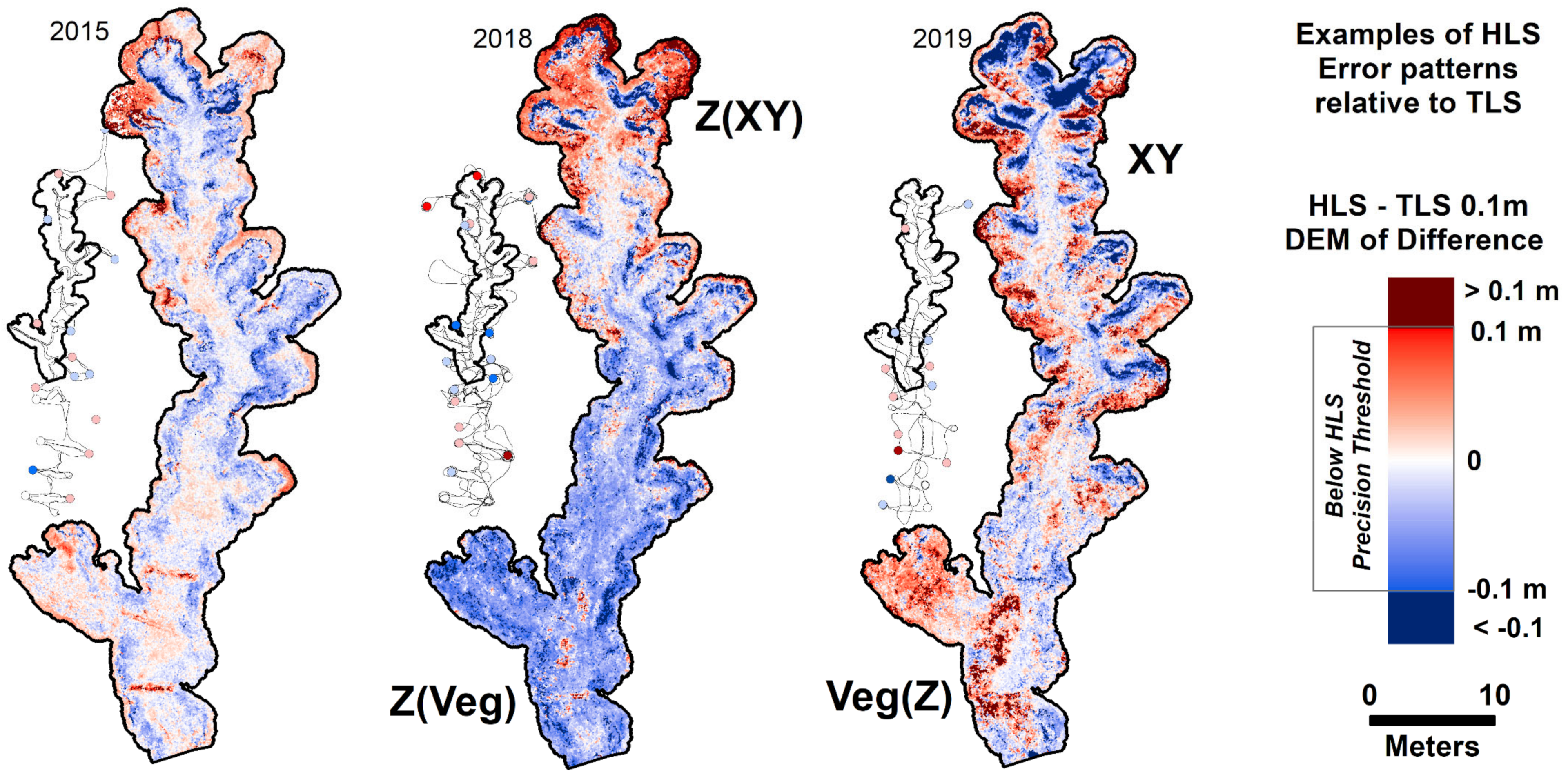
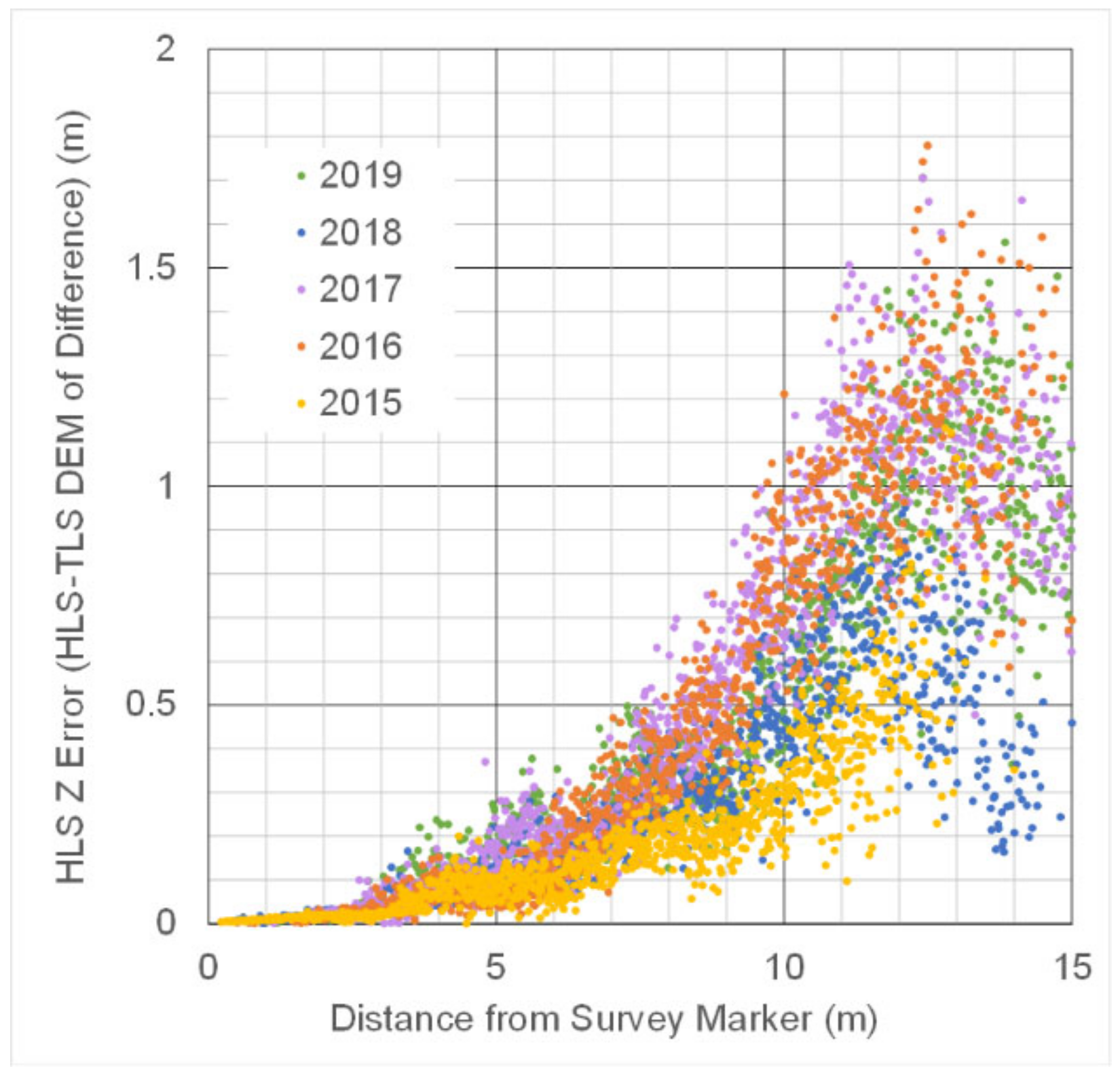
3.2.1. Precision and Broadscale Distortion

The duplicate HLS surveys conducted on 4 November 2015 were processed in an identical manner and referenced using an identical set of survey markers. As with the annual HLS surveys, 10 cm DEMs were generated using the HLS workflow in Figure 2. Ucrit was calculated to be 0.0911 from the DEM of difference of these duplicate scans within the 2015 gully area and was consistent with the manufacturers’ estimate of HLS precision. Based on Ucrit, the threshold for detection of change in HLS was rounded to a slightly more conservative value of 0.1 m for the conditions of this study. In comparison, Ucrit for the TLS scanner had previously been determined to range between 0.134 m at another gully site [28] and ± 0.05–0.067 m at this study gully (based on repeat scans from 2015 gridded to 5 cm DEMs [32]).
Rigid Transform matrices applied to the raw HLS point cloud to convert to reference coordinates are detailed in Table A2 in Appendix B. Table 2 summarises the rigid transform RMSE and XYZ residual error characteristics of HLS scans for each year (A in Figure 2 and Figure 4). Between 16 and 25 survey marker points were captured in each survey, but the same markers were not always scanned. Very few (at most 3) of the marker points needed to be removed to achieve a target RMSE of less than 0.1 m over the length of the HLS gully scan (100 m), suggesting that scan distortions are low and that the GIS method has accurately detected the locations of most survey markers. Transform residuals were also derived for the two individual scans making up the 2018 merge and showed that, despite different trajectory paths, both exhibited similar spatial patterns of residuals and overall RMSE to each other and to the merged survey (0.098 m and 0.097 m). This suggested that the main influence on transform errors was specific to the year rather than the scan path trajectory. There was evidence of systematic increases in X and Y residuals (either positive or negative) at the upstream and downstream ends of the scan, consistent with a slight shrinkage or expansion of the scan distances relative to RTK. This type of distortion cannot be fixed with an unscaled rigid transform, but was generally less than 0.1 m. In comparison, rigid transform errors for TLS (based on the 5 TLS bases as survey markers) averaged 0.005, 0.007, and 0.014 m in X, Y and Z, respectively for the 2019 survey, with an overall RMSE of 0.017 m. TLS for other years had similar RMSE, all being less than 0.02 m. Although, it was observed that RMSE in HLS residuals could be reduced to similar levels when the number of survey markers used was similarly reduced.
There appears to be general trend of increasing transform residual RMSE from 2015 to 2019 in Table 2. This corresponds with a trend of scanning times closer to the end of the wet season in March (Table 1). The HLS survey for 2015 was conducted at the end of the dry season (November) when ground vegetation cover was very sparse. The 2016 scan was conducted earlier (August) but still well into the dry season. From 2017 to 2019 surveys were being conducted in April due to reporting deadlines, and vegetation was still thick from the wet (growing) season.

3.2.2. Error in Gully Morphology

Cross section profiles from HLS 10 cm DEMs (B in Figure 2 and Figure 4) reproduced the shape of the RTK cross sections profiles (G in Figure 3 and Figure 4) with an RMSE of 0.092 m and a strong 1:1 linear relationship (R2 = 0.988) for all profiles in all years of RTK and HLS (2015 to 2018, 573 points). This gives confidence that HLS DEMs can reliably measure broad metrics such as gully width and depth to within the HLS estimated precision of 0.1 m.
HLS gully area, maximum gully depth and gully volume (C and D in Figure 2 and Figure 4, and Figure 5b) were consistently over-predicted compared to TLS (J and K in Figure 3 and Figure 4). However, were, on average, within 5–6% of TLS (Table 3).
Within the gully, errors in HLS DEMs (B in Figure 2 and Figure 4) relative to TLS DEMs (I in Figure 3 and Figure 4) were evaluated using an HLS-TLS DoD and were generally within the expected precision of HLS (Figure 6), although we observed a number of patterns to these errors which are illustrated in Figure 6 and described below:
  • XY–XY offset of HLS relative to TLS evident in steep areas as paired red-blue “shadows”. paired positive and negative (red-blue) “shadow” artefacts in steep walled areas on opposite sides of the gully.
  • Z–Z offset of HLS relative to TLS evident as uniform coloration in the DoD.
  • Veg—Vegetation artefacts evident as highly textured “blobs” of red, where HLS has been unable to penetrate dense vegetation and/or is affected by localized low point density.
There appears to be a similarity in spatial distributions of transform residuals (insets in Figure 6) and HLS-TLS DoD errors suggesting distortions relate to HLS, not the validation data.
On the flat areas outside the gully, the HLS-TLS DoD has the lowest errors near the survey markers (Figure 7). The area around each survey marker has not been cleared of vegetation, so the pattern of errors relates almost exclusively to scanner view angle and point density: low point density and flat view angle will result in a higher frequency of vegetation canopy artefacts at increasing distances. Figure 7 gives confidence that ground is being reliably detected in HLS scans at distances of up to 3 m around survey markers, equating to about 2 m from the scanner itself. More direct measurements of DoD values with distance from the scanner trajectory were inconclusive as areas away from reference markers were impacted by scan distortions and steep terrain.

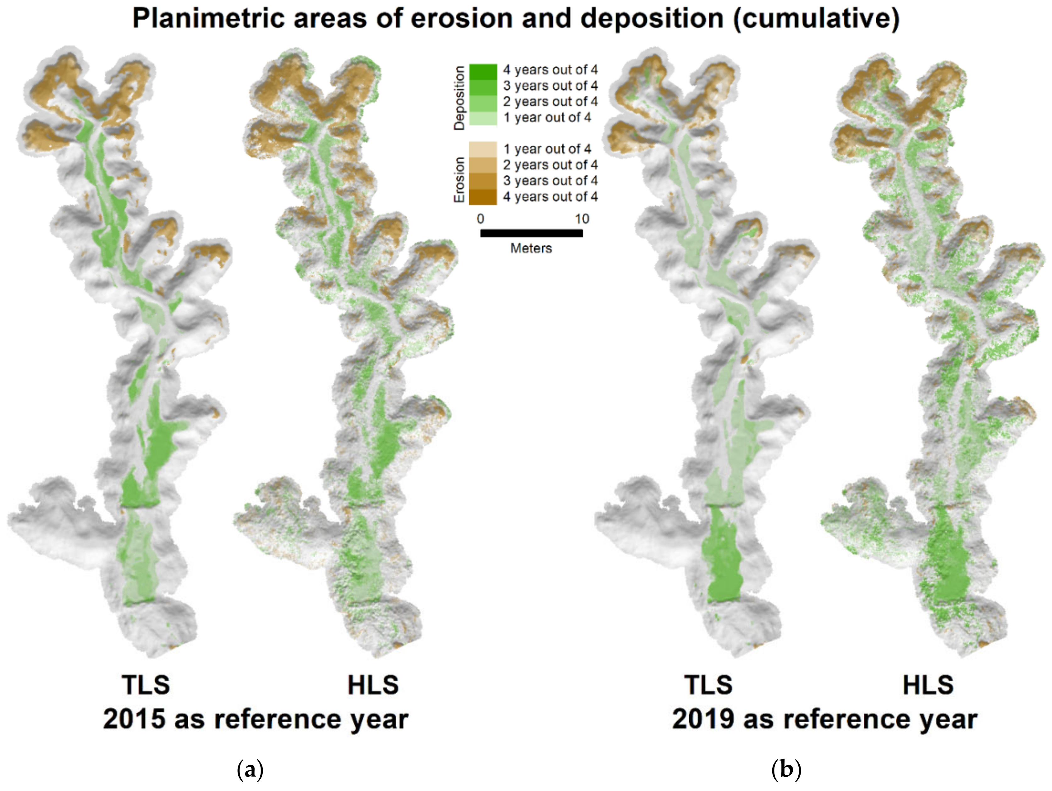
3.3. HLS Error Detecting Change in Gullies

3.3.1. Headcut Extension Compared to RTK

The shape of the HLS headcut rim polyline derived using the HLS workflow (E in Figure 2 and Figure 5c) was similar to that of the RTK survey for the same year (H in Figure 3 and Figure 5c), but with an upstream offset due to the HLS DEM being unable to represent the headcut overhang. Despite this offset, the distance from a fixed point to the apex of the headcut HLS polyline (Figure 5c), the undercut in Figure 1) is highly correlated to the distance as measured using RTK (Figure 5c), the overhang in Figure 1) with an r2 of 0.99, slope of 1.08, and intercept of −0.49 (n = 4). The equation confirms that the overhang is receding at the same rate as the undercut and that the two are offset by a consistent distance of 0.5 m. Annual headcut retreat rates based on this linear distance measure are between 0.23 and 0.77 m/y for HLS and between 0.38 and 0.54 m/y for RTK). Consequently, average annual headcut extension (average movement of headcut polyline) derived from HLS (E in Figure 2 and Figure 5c) is highly correlated with RTK with a line of best fit with r2 of 0.95 and slope of 1.05, with average error of 0.003 m (range of −0.045 (−36%) to 0.079 m (+47%) and an RMSE of 0.035 m (n = 6). Annual change in headcut area is also strongly correlated to RTK, despite areas are being overestimated by approximately 20% (line of best fit: r2 = 0.86, slope = 1.18), with an average error of 0.249 m2 from a range of −0.196 m2 (−22%) to 0.753 m2 (+66%) and RMSE of 0.434 m2) (n = 6).

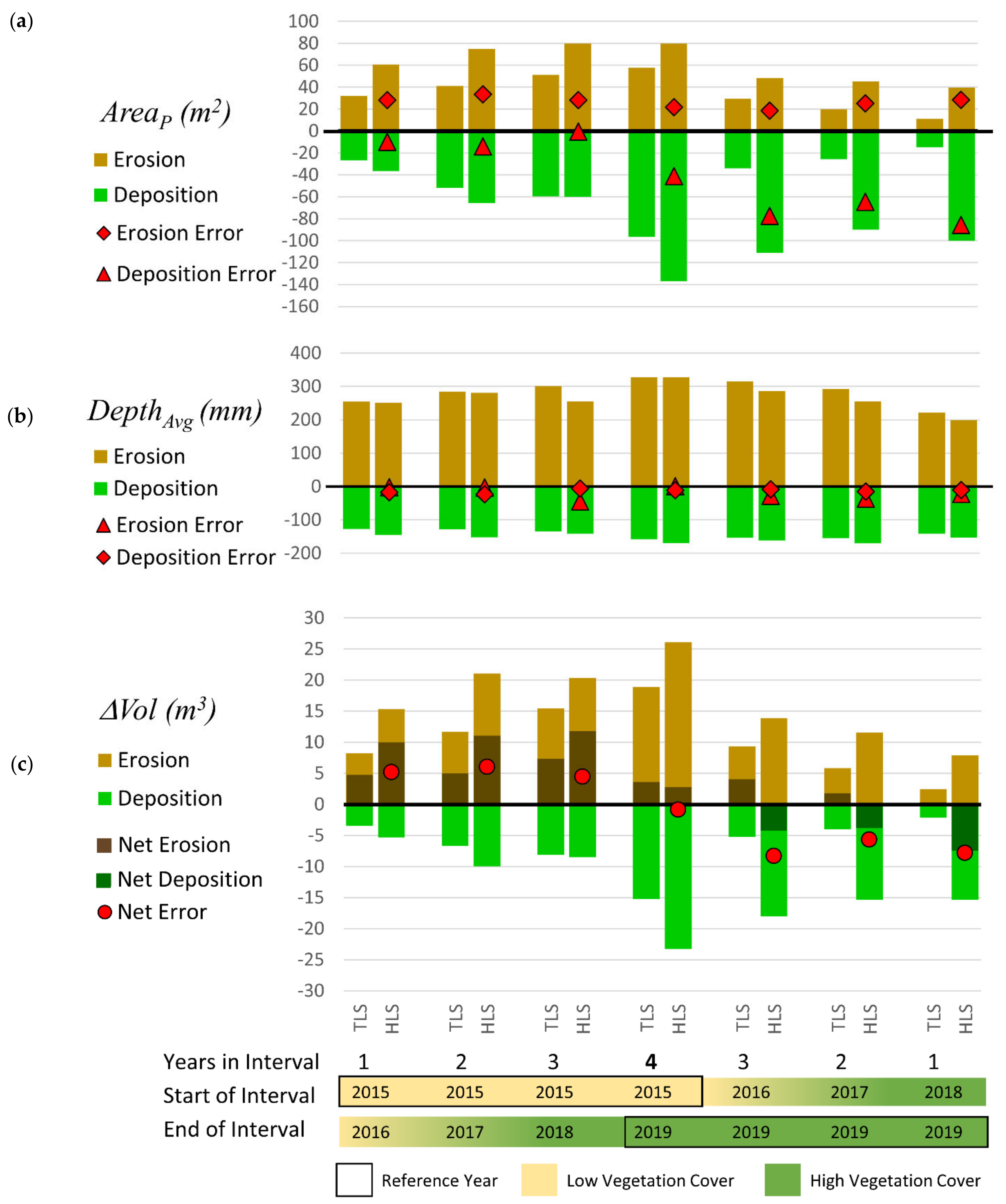
3.3.2. Volumetric Change (Net Erosion Compared to TLS)

The TLS validation data show that planimetric areas of erosion and deposition in the gully grew by 58 m2 and 96 m2, respectively in the four years from 2015 to 2019 (Table 4). Erosion areas also deepened on average by 328 mm and deposition increased by 158 mm. Consequently, overall volumes of erosion and deposition also grew. However, the volumes of erosion and deposition over this 4-year period are of similar magnitude to each other, being 18.9 and 15.2 m3, respectively, resulting in a smaller magnitude volumetric change of 3.7 m3 net erosion over the 60 m length of the gully. This means that detecting net volumetric change accurately may challenging.
Cumulative patterns of deposition and erosion in HLS and TLS over the 5-year period appear similar (Figure 8). However, AreaP(eros) was consistently overestimated relative to TLS by, on average, 27 m2 (n = 8) regardless of reference year or interval and AreaP(dep) was overestimated by, on average, 66 m2 (n = 4) when 2019 was used as the reference year or 16 m2 (n = 4) when 2015 was used as the reference year (Figure 9a) and Table A3 from the Appendix C). DepthAvg(eros) was consistently underestimated by HLS relative to TLS, although by less than 46 mm (average error 20 mm, n = 8). DepthAvg(dep) was consistently overestimated by HLS relative to TLS, but also by less than 24 mm (average error 14 mm, n = 8) regardless of the interval in years (Figure 9b) and Table A4). Figure 9c and Table A5 show the consequences of these errors in DepthAvg and AreaP on HLS’s ability to estimate net volume change ΔVol (4). For each reference year, ΔVol errors remain relatively constant for all intervals of less than 4 years: averaging +5.3 m3 for intervals using 2015 as the reference year, and −7.2 m3 for intervals using 2019 as the reference year. For the full 4-year interval 2015–2019 the error is lower at −0.8 m3, a 23% underestimate compared to TLS. The reduction in error for the 4-year interval compared to smaller intervals should be interpreted with caution, as the errors in volumes of erosion and deposition when considered separately are still quite large (7.2 m3 (38%) and 8.1 m3 (53%), respectively), effectively offsetting each other.
Errors in HLS ΔVol are highly correlated to errors in AreaP as can be seen in the similarity of patterns in Figure 9a,c, with r2 = 0.98 and r2 = 1.0, respectively for AreaP(eros) and AreaP(dep), respectively. There was no correlation between error in ΔVol and error in DepthAvg (r2 = 0.15 and r2 = 0.07, respectively).
Figure 8b shows additional areas of erosion or deposition compared to TLS (Figure 8a). These additional areas occur in similar locations to HLS-TLS DoD errors in Figure 6, particularly when they occur in the reference year. While subtle, such errors are contributing to significant over-estimation of the planimetric area of both erosion and deposition particularly for 2019. Additionally, this is propagating into estimates of volumetric change.

4. Discussion and Recommendations

4.1. HLS Errors and Implications for Change Detection amd Monitoring Frequency

All HLS errors measured at the gully are summarised in Table 5. RMSE of residuals from the rigid transforms showed that XYZ errors in individual HLS scans were below 0.1 m over the 100 m length of the scans, consistent with the estimated HLS precision from Ucrit. Gully shape such as area, depth, volume and cross sections profiles (and by inference, width and slope) were reproduced by the HLS 10 cm DEMs to within 5–6% of TLS and 0.1 m of RTK measurements. Overall, these errors suggest that HLS can be used successfully for measuring the morphology of gullies as well as the retreat rates of the headcut to within the 0.091 m precision and 0.1 m resolution of the workflow products. A previous erosion pin study at this gully [13] determined that annual changes in cross section profiles downstream of the headcut were between 2.2 and 7.2 mm for gully walls and 3 mm for gully floors in gullies without check dams, confirming that it would take more than the 4 years at our study site to reliably detect changes in the gully below the headcut unless we were able to improve the precision of HLS. It is worth noting that such small erosion rates are also at the limits of detectability for TLS and RTK. So the fact that we are detecting similar patterns of erosion and deposition between HLS and TLS DEMs (Figure 8) is encouraging.
Comparison of HLS 10 cm DEMs with equivalent 10 cm DEMs from TLS demonstrated that errors, while small, are dominated by systematic XY and Z distortions with some minor vegetation artefacts (Figure 6). Systematic distortions appear to originate from HLS rather than TLS as there are similarities in the spatial patterns of errors in the residuals of RTK derived transforms (insets in Figure 6). These distortions propagated into the HLS DEMs of difference used for estimates of volumetric change between years. DepthAvg is sensitive to Z distortions. However, planimetric area (AreaP) is sensitive to distortions in all directions: Z distortion in flat areas of the gully, in combination with the application of a threshold of detection, can expand or contract the area of erosion or deposition features, while XY misregistration displaces steep gully features resulting in paired positive and negative artefacts, which may be interpreted erroneously as additional areas of erosion and deposition. Reducing distortions in HLS scans is thus important for improving our ability to use HLS DEMs of difference for change detection.
There was a trend to higher transform RMSEs in 2017, 2018 and 2019, despite a high degree of confidence in ground detection near survey markers (Figure 7). These years were scanned closer to the end of the wet season than 2015 and 2016 and ground vegetation cover was denser. Thus, we speculate that vegetation creates a more complex scanning environment that subtly impacts the accuracy of SLAM’s object recognition, resulting in the subtle systematic distortions that have then contributed to errors in volumetric change estimates. Vegetation anomalies were also present in DEMs derived from more heavily vegetated scans (Veg in Figure 6). Thus, surveying once only at the time of year with lowest ground vegetation cover is highly recommended.
The accuracy of volumetric change estimates from DEMs of difference can also be affected by the choice of a reference year, as distortions or vegetation effects in the reference year may be propagated through all volumetric change estimates. This is evident from the increase in the magnitude of errors when 2019 is used as the reference year for volumetric change as opposed to 2015 (Figure 9, Table A5).

4.2. Comparison of HLS with Other Gully Monitoring Approaches

Table 6 details a range of methods that have been used for measuring and monitoring linear gullies. Monitoring needs to account for all sources of erosion and deposition within the gully. Table 6 shows that while erosion pins are the most precise method, they can only capture small (mm-scale) changes in gully walls and floors. With RTK, approximately 300–500 points can be collected within a survey timeframe of 1½ h, but features are selected at the operator’s discretion and thus requires a moderate level of skill to understand the key features of the gully required. Wilkinson et al. [13] used a combination of erosion pins and RTK to estimate volume loss from gullies and interpret these results in the context of remediation. However, with improvements in technology, most current methods (all other methods listed in Table 6) generate semi-random point clouds which must then be classified into ground and non-ground returns before being converted into an object such as a DEM representative of the gully. A DEM is not a complete 3D representation of the gully, in that it is unable to reproduce the overhang rim geometry common in headcuts but will, instead, capture the shape of the undercut wall beneath the rim. However, the simplicity of DEMs is appealing as they are both easy to generate, consistent in structure and easy to analyse. All point cloud methods require a moderate skill-level to process into a DEM or other products. Structure from Motion (SfM) is the cheapest point-cloud method in terms of equipment and software purchase, but processing is time consuming, and the data can be impacted by vegetation and shadow. TLS systems such as the Reigl are the gold standard, but require a high operator skill level, are time consuming, and the systems are expensive to purchase. Airborne lidar is the gold standard for broadscale mapping of large areas (>10 km2) but is not suitable for monitoring changes in individual gullies, except where the gullies are large and complex and have very high rates of erosion (e.g., >0.2 m). HLS benefits from high levels of detail like TLS, but has the benefit of ease of use and speed of field survey at a competitive price. These attributes also mean HLS offers an attractive alternative to TLS for ground truth dataset for airborne lidar [33] surveys which are used extensively for gully mapping and monitoring in GBR catchments.

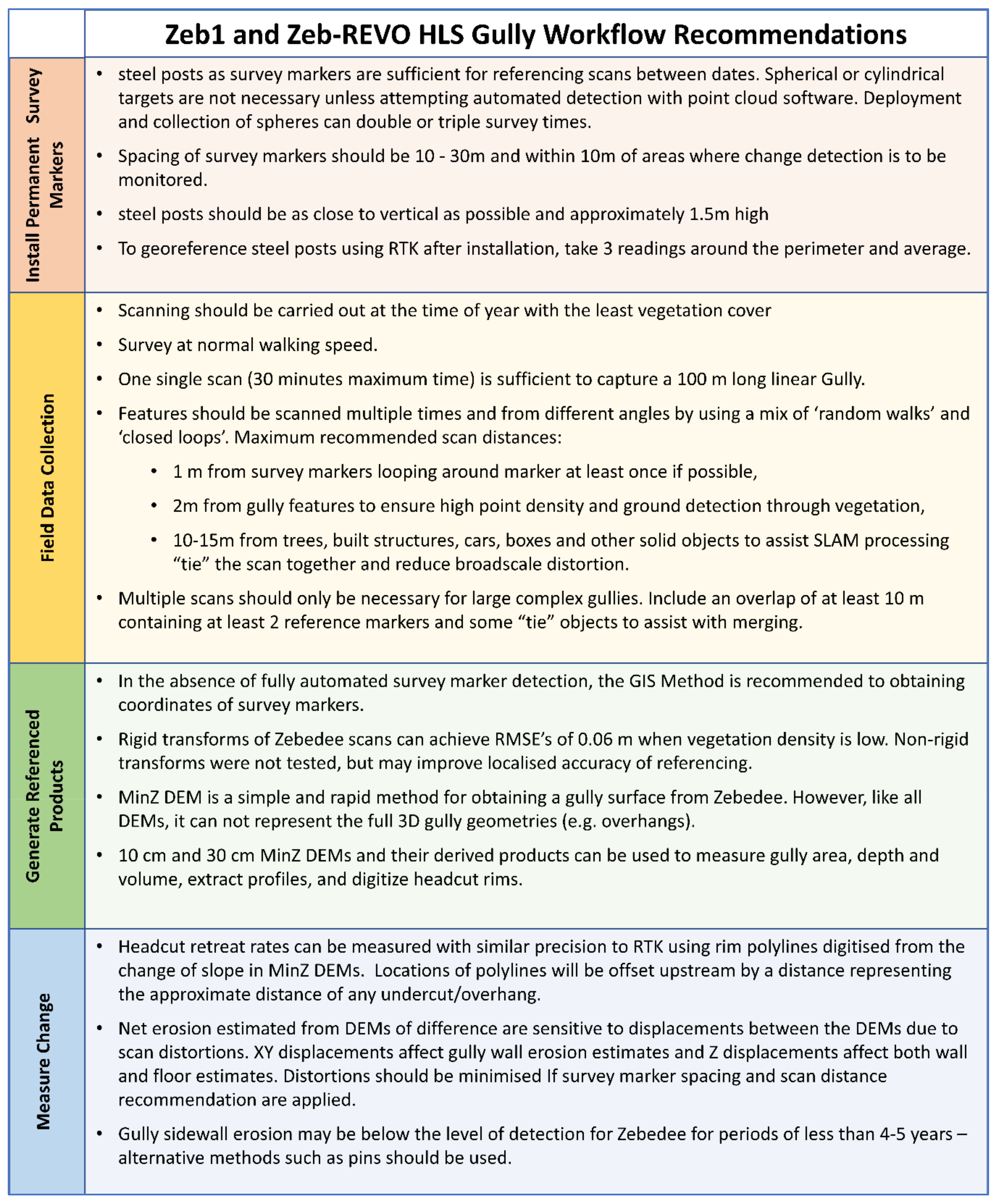
4.3. Recommendations for Application of HLS Gully Workflow

The Zeb1 and Zeb-REVO HLS gully workflow is detailed in Figure 2 and described in the Methods section. Once survey markers (steel posts) are installed, a gully of 100–150 m long can be scanned or re-scanned in 30 min. Steel posts, once installed, required no further setting up prior to survey, reducing survey time to almost 1/3 the time required if target deployment and collection had been required (e.g., for TLS and RTK bases). If real-world coordinates for the survey markers have not been previously surveyed using a GPS (e.g., RTK), raw locations from a previous scan can be used as a reference. Generating a referenced point cloud and gridded products using the HLS workflow took about 1 h. Additional products such as gully area and volume and headcut polylines involved some user intervention and added at most an extra hour to processing. Recommendations regarding how to apply the HLS workflow are detailed in Figure 10 and are based on 5 years of gully survey at the study site and other gullies in the region.

4.4. Areas of Future Improvement and Research

This study has quantified errors in measuring gully morphology and erosion over a four year period using two models of hand-held laser scanner. There are several areas of further research that could improve our understanding of these errors:
  • Re-evaluate HLS errors using the new GeoSLAM reference plate technology: In mid-2020 a reference plate was introduced by GeoSLAM which makes it possible to “tag” the location of survey markers during scanning and apply rigid or non-rigid transforms automatically during GeoSLAM processing. This has potential to replace the GIS Method and Referencing steps in the HLS workflow (Figure 2). The reference plate method cannot be applied retrospectively to historical scans and improvements in the accuracy of new scans would need to be re-assessed.
  • Re-evaluate HLS errors based on non-rigid transforms or localized corrections: Subtle broadscale distortions in HLS scans were the major contributor to error in estimating volumes of erosion and deposition. Distortions may, in theory, be reduced by using non-rigid transforms or localized corrections. Non-rigid point cloud transforms are possible in GeoSLAM’s latest Hub software for scans where the reference plate has been used. Alternatively, methods such Particle Image Velocimetry [36] and Fourier analysis could potentially also be used to detect localised distortions in XY and Z (respectively) between two DEMs without the need for extra survey markers, although care should be taken to avoid “correcting” real gully morphological changes.
  • Evaluate in more detail the ability of HLS to detect gully wall erosion. Erosion pin measurements at this study site suggest 4-year erosion rates were below the limits of detection by HLS. However, such gully wall erosion can be significant across large areas of gully wall [13]. Improvements in the detection of gully wall erosion may also improve the estimation of volumetric change.

5. Conclusions and Recommendations

Detailed HLS workflow for gully monitoring and recommendations for its application were presented in this paper. Error analysis of the workflow products showed that, with an accuracy around 0.1 m, HLS gully surveying is almost as accurate as TLS and RTK for gully morphology and change detection at annual to four-year intervals. HLS surveys were fast and easy, with a field technician able to complete a 100 m long survey of a linear gully in approximately 30 min by walking with the scanner in overlapping patterns, capturing key gully features and permanent reference markers. As such, HLS offers an attractive, more portable, alternative to TLS for calibration or ground truth of airborne lidar surveys used for broad-scale gully mapping and monitoring in GBR catchments.
For repeat HLS surveys of individual gullies, an interval of four years provided significant reduction in uncertainty for estimation of volumetric change compared to one-year intervals. However, one year was sufficient to measure headcut extension and detect spatial patterns of erosion and deposition, particularly if surveys are conducted when vegetation cover is low. Reporting is often required annually for remediation projects. For the Great barrier Reef catchments of Queensland, where rainfall is highly seasonal, it is not recommended to survey more frequently than once a year and where possible, this surveys should be conducted late in the dry season when vegetation cover is lowest. For remediated gullies, where erosion rates may be low or deposition significant, HLS surveys should span at least four years if quantification of net volumetric change is required.

Author Contributions

Conceptualization, A.K.-H., A.H. and S.N.W.; Data curation, A.H. and T.L.; Formal analysis, A.K.-H. and A.H.; Funding acquisition, R.B. and S.N.W.; Investigation, A.K.-H., A.H., S.N.W. and T.L.; Methodology, A.K.-H., A.H. and T.L.; Project administration, R.B.; Resources, A.H. and R.B.; Software, A.K.-H. and T.L.; Supervision, R.B.; Validation, A.K.-H. and A.H.; Visualization, A.K.-H.; Writing—original draft, A.K.-H. and S.N.W.; Writing—review and editing, A.H., R.B. and T.L. All authors have read and agreed to the published version of the manuscript.

Funding

This research was funded by from the Australian Government’s National Environmental Science Program Tropical Water Quality Hub (Projects 2.14 and 5.9).

Institutional Review Board Statement

Not applicable.

Informed Consent Statement

Not applicable.

Data Availability Statement

The data presented in this study are available on request from the corresponding author. The data are not publicly available due to privacy.

Acknowledgments

This study was supported by the CSIRO, with additional funding from the Australian Government’s National Environmental Science Program Tropical Water Quality Hub (Projects 2.14 and 5.9) and Caring for Country Program (grant A0000010417G).

Conflicts of Interest

The authors declare no conflict of interest.

Appendix A. GeoSLAM Settings

Table A1 below shows the settings used in GeoSLAM processing. These are not all the default settings. The reasons for these choices were not always intuitive and were determined through trial and error and advice from developers in order to generate the best point cloud possible in the complex outdoor environment of a gully (e.g., Start/Finish Closed Loop actually had trouble reconnecting, leaving survey start and end objects adrift). Descriptions of these options can be found in the GeoSLAM User Guide: https://download.geoslam.com/docs/zeb-revo-rt/ZEB-REVO%20RT%20User%20Guide%20V1-0-1.pdf (Accessed on 27 September 2017).
Table A1. Processing options used in GeoSLAM V 4.1.1 to give best results in gullied environment.
GeoSLAM Processing OptionDefaultUsed
Local Convergence Threshold (0)00
Local Windows Size (0)44
Local Voxel Density (1)12
Local Rigidity (0)00
Modify Bounding Box (False)FalseFalse
Process in Reverse (False)FalseFalse
Conservative Outlier Pruning (False)FalseTrue
Large Range Filter Slope (False)FalseTrue
End Processing Early (False)FalseFalse
Place Recognition (False)FalseTrue
Prioritise Planar Surface (False)FalseFalse
Start/Finish–Closed loop (True)TrueFalse

Appendix B. Transformation from Raw HLS Scan Coordinates to GDA94 MGA55

HLS point clouds were transformed from raw HLS scan coordinates to GDA94 MGA55 by pairing the RTK reference marker coordinates to the corresponding reference marker HLS raw scan coordinates (obtained using the GIS Method) and deriving the transformation matrices as shown in Table A2.
Table A2. Transformation matrices applied to each HLS scan point cloud as part of Step 2. For the transformation matrix, R is a standard 3 × 3 rotation matrix and T is a translation vector. Let P be a 3D point, the transformed point P’ will be such that: P’ = R.P + T. E = error.
Transformation Matrix2015
R11R12R13Tx9.99 E − 0.13.76 E − 0.2−1.00 E − 0.3448,992.03
R21R22R23Ty−3.76 E − 0.29.99 E − 0.12.68 E − 0.57,800,429.24
R31R32R33Tz1.00 E − 0.31.09 E − 0.51.00 E + 0.0326.36
00010001
20162017
1.00 E + 0.0−1.12 E − 0.22.80 E − 0.3448,993.50−9.93 E − 0.11.17 E − 0.11.16 E − 0.4448,993.90
1.12 E − 0.21.00 E − 0.02.80 E − 0.37,800,422.75−1.17 E − 0.1−9.93 E − 0.11.25 E − 0.37,800,430.97
−2.83 E − 0.3−2.77 E − 0.31.00 E + 0.0326.062.62 E − 0.41.23 E − 0.31.00 E + 0.0326.35
00010001
20182019
9.52 E − 0.13.05 E − 0.1−3.05 E − 0.3449,024.15−9.82 E − 0.1−1.89 E − 0.11.87 E − 0.3449,010.55
−3.05 E − 0.19.52 E − 0.1−1.45 E − 0.37,800,428.761.89 E − 0.1−9.82 E − 0.11.91 E − 0.37,800,439.44
2.46 E − 0.32.32 E − 0.31.00 E + 0.0327.321.48 E − 0.32.23 E − 0.31.00 E − 0.0327.52
00010001

Appendix C. Tables of HLS Volumetric Change and Errors

The tables below can be cross-referenced against equivalent TLS measurements reported in Table 4. Data below are represented graphically in Figure 9.
Table A3. Planimetric area AreaP of deposition and erosion for each HLS year interval. Errors are relative to equivalent measures from TLS (Table 4). Eros = Areas of Erosion, Dep = Areas of Deposition. Bolded year is reference year used. Data below is represented graphically in Figure 9.
AreaP (m2)Error (m2)Error (%)
IntervalNo YearsErosDepErosDepErosDep
2015–2016160.736.528.59.689%36%
2015–2017274.965.633.913.783%26%
2015–2018379.659.928.40.256%0%
2015–2019479.7137.122.140.738%42%
2016–2019348.3111.018.877.164%227%
2017–2019245.390.025.464.3128%251%
2018–2019139.8100.128.785.3259%575%
Table A4. Average depth DepthAvg in areas of deposition and erosion for each HLS year interval. Errors are relative to equivalent measures from TLS (Table 4). Eros = Areas of Erosion, Dep = Areas of Deposition. Bolded year is reference year used. Data below is represented graphically in Figure 9.
IntervalNo YearsDepthAvg (mm)Error (mm)Error (%)
ErosDepErosDepErosDep
201520161252145−318−1%14%
2015–20172281152−424−1%18%
2015–20183255142−467−15%5%
2015–201943271700120%8%
2016–20193287162−299−9%6%
2017–20192255170−3716−13%10%
2018–20191198153−2311−10%8%
Table A5. Volumetric change ΔVol (m3) in areas of deposition and erosion for each HLS year interval. Errors are relative to equivalent measures from TLS (Table 4). Eros = erosion, Dep = deposition, Net = Erosion–Deposition. Bolded year is reference year used. Data below are represented graphically in Figure 9.
IntervalNo YearsΔVol (m3)Error (m3)Error (%)
ErosDepNetErosDepNetErosDepNet
2015–2016115.35.310.07.11.95.287%55%109%
2015–2017221.110.011.19.43.36.180%50%120%
2015–2018320.38.511.84.90.44.532%5%61%
2015–2019426.123.32.87.28.1−0.838%53%−23%
2016–2019313.818.0−4.24.612.8−8.249%246%−203%
2017–2019211.515.3−3.85.711.4−5.699%286%−307%
2018–201917.915.3−7.45.413.2−7.8222%628%−2235%

References

  1. The State of Queensland. Reef Water Quality Protection Plan 2013; Reef Water Quality Protection Plan Secretariat: Brisbane, Australia, 2013. [Google Scholar]
  2. The State of Queensland. Reef 2050 Water Quality Improvement Plan 2017–2022; Reef Water Quality Protection Plan Secretariat: Brisbane, Australia, 2017. [Google Scholar]
  3. Wilkinson, S.N.; Hancock, G.J.; Bartley, R.; Hawdon, A.A.; Keen, R.J. Using sediment tracing to assess processes and spatial patterns of erosion in grazed rangelands, Burdekin River basin, Australia. Agric. Ecosyst. Environ. 2013, 180, 90–102. [Google Scholar] [CrossRef]
  4. Wilkinson, S.N.; Olley, J.M.; Furuichi, T.; Burton, J.; Kinsey-Henderson, A.E. Sediment source tracing with stratified sampling and weightings based on spatial gradients in soil erosion. J. Soils Sediments 2015, 15, 2038–2051. [Google Scholar] [CrossRef]
  5. Wilkinson, S.N.; Hairsine, P.B.; Brooks, A.; Bartley, R.; Hawdon, A.; Pietsch, T.; Shepherd, B.; Austin, J. Gully and Stream Bank Toolbox (2nd Edition): A Technical Guide for the Reef Trust Phase IV Gully and Stream Bank Erosion Control Program; Commonwealth of Australia: Canberra, Australia, 2019; 94p. [Google Scholar]
  6. Giménez, R.; Marzolff, I.; Campo, M.A.; Seeger, M.; Ries, J.B.; Casalí, J.; Álvarez-Mozos, J. Accuracy of high-resolution photogrammetric measurements of gullies with contrasting morphology. Earth Surf. Process. Landf. 2009, 34, 1915–1926. [Google Scholar] [CrossRef]
  7. Castillo, C.; Pérez, R.; James, M.R.; Quinton, J.N.; Taguas, E.V.; Gómez, J.A. Comparing the Accuracy of Several Field Methods for Measuring Gully Erosion. Soil Sci. Soc. Am. J. 2012, 76, 1319–1332. [Google Scholar] [CrossRef] [Green Version]
  8. Goodwin, N.R.; Armston, J.D.; Muir, J.; Stiller, I. Monitoring gully change: A comparison of airborne and terrestrial laser scanning using a case study from Aratula, Queensland. Geomorphology 2017, 282, 195–208. [Google Scholar] [CrossRef]
  9. Koci, J.; Jarihani, B.; Leon, J.X.; Sidle, R.C.; Wilkinson, S.N.; Bartley, R. Assessment of UAV and Ground-Based Structure from Motion with Multi-View Stereo Photogrammetry in a Gullied Savanna Catchment. ISPRS Int. J. Geo-Inf. 2017, 6, 328. [Google Scholar] [CrossRef] [Green Version]
  10. Abegg, M.; Kukenbrink, D.; Zell, J.; Schaepman, M.E.; Morsdorf, F. Terrestrial Laser Scanning for Forest Inventories Tree Diameter Distribution and Scanner Location Impact on Occlusion. Forests 2017, 8, 184. [Google Scholar] [CrossRef] [Green Version]
  11. Puente, I.; Gonzalez-Jorge, H.; Martinez-Sanchez, J.; Arias, P. Review of mobile mapping and surveying technologies. Measurement 2013, 46, 2127–2145. [Google Scholar] [CrossRef]
  12. Glennie, C.; Brooks, B.; Ericksen, T.; Hauser, D.; Hudnut, K.; Foster, J.; Avery, J. Compact Multipurpose Mobile Laser Scanning System - Initial Tests and Results. Remote Sens. 2013, 5, 521–538. [Google Scholar] [CrossRef] [Green Version]
  13. Wilkinson, S.N.; Kinsey-Henderson, A.E.; Hawdon, A.A.; Hairsine, P.B.; Bartley, R.; Baker, B. Grazing impacts on gully dynamics indicate approaches for gully erosion control in northeast Australia. Earth Surf. Process. Landf. 2018, 43, 1711–1725. [Google Scholar] [CrossRef]
  14. Kroon, F.; Kuhnert, P.; Henderson, B.; Wilkinson, S.; Henderson, A.; Abbott, B.; Brodie, J.; Turner, R. River loads of suspended solids, nitrogen, phosphorus and herbicides delivered to the Great Barrier Reef lagoon. Mar. Pollut. Bull. 2012, 65, 167–181. [Google Scholar] [CrossRef]
  15. Bartley, R.; Corfield, J.P.; Hawdon, A.A.; Kinsey-Henderson, A.E.; Abbott, B.N.; Wilkinson, S.N.; Keen, R.J. Can changes to pasture management reduce runoff and sediment loss to the Great Barrier Reef? The results of a 10-year study in the Burdekin catchment, Australia. Rangel. J. 2014, 36, 67–84. [Google Scholar] [CrossRef] [Green Version]
  16. Bosse, M.; Zlot, R.; Flick, P. Zebedee: Design of a Spring-Mounted 3-D Range Sensor with Application to Mobile Mapping. IEEE Trans. Robot. 2012, 28, 1104–1119. [Google Scholar] [CrossRef]
  17. Sirmacek, B.; Shen, Y.; Lindenbergh, R.; Zlatanova, S.; Diakite, A.; Baatz, R. Comparison of ZEB1 and Leica C10 Indoor Laser Scanning Point Clouds. In Proceedings of the XXIII ISPRS Congress, Prague, Czech Republic, 12–19 July 2016. [Google Scholar]
  18. Thomas, J.B.; Dewez, E.P.; Degas, M.; Richard, T.; Pannet, P. Handheld Mobile Laser Scanners Zeb-1 and Zeb-Revo to map an underground quarry and its above-ground surroundings. In Proceedings of the 2nd Virtual Geosciences Conference, VGC 2016, Bergen, Norway, 22–23 September 2016. [Google Scholar]
  19. Marselis, S.M.; Yebra, M.; Jovanovic, T.; van Dijk, A. Deriving comprehensive forest structure information from mobile laser scanning observations using automated point cloud classification. Environ. Model. Softw. 2016, 82, 142–151. [Google Scholar] [CrossRef]
  20. Zlot, R.; Bosse, M.; Greenop, K.; Jarzab, Z.; Juckes, E.; Roberts, J. Efficiently capturing large, complex cultural heritage sites with a handheld mobile 3D laser mapping system. J. Cult. Herit. 2014, 15, 670–678. [Google Scholar] [CrossRef]
  21. James, M.R.; Quinton, J.N. Ultra-rapid topographic surveying for complex environments: The hand-held mobile laser scanner (HMLS). Earth Surf. Process. Landf. 2014, 39, 138–142. [Google Scholar] [CrossRef] [Green Version]
  22. Ryding, J.; Williams, E.; Smith, M.J.; Eichhorn, M.P. Assessing Handheld Mobile Laser Scanners for Forest Surveys. Remote Sens. 2015, 7, 1095–1111. [Google Scholar] [CrossRef] [Green Version]
  23. GeoSLAM. ZEB-REVO Users Manual V 3.0.0.; GeoSLAM: Nottingham, UK, 2017. [Google Scholar]
  24. Hokuyo. Scanning Laser Range Sensor UTM-30LX-F SPECIFICATIONS. Available online: https://hokuyo-usa.com/application/files/7015/9111/2563/UTM-30LX-F_Specifications.pdf (accessed on 1 August 2021).
  25. Microstrain. 3DM-GX2 Technical Product Overview. Available online: http://files.microstrain.com/3dm-gx2_datasheet_v1.pdf (accessed on 1 August 2021).
  26. ASPRS. LAS Specification Version 1.2, American Society for Photogrammetry and Remote Sensing (ASPRS). Available online: https://www.asprs.org/wp-content/uploads/2010/12/asprs_las_format_v12.pdf (accessed on 30 April 2021).
  27. Wells, R.R.; Momm, H.G.; Castillo, C. Quantifying uncertainty in high-resolution remotely sensed topographic surveys for ephemeral gully channel monitoring. Earth Surf. Dynam. 2017, 5, 347–367. [Google Scholar] [CrossRef] [Green Version]
  28. Goodwin, N.R.; Armston, J.; Stiller, I.; Muir, J. Assessing the repeatability of terrestrial laser scanning for monitoring gully topography: A case study from Aratula, Queensland, Australia. Geomorphology 2016, 262, 24–36. [Google Scholar] [CrossRef]
  29. Burrough, P.A.; McDonell, R.A. Principles of Geographical Information Systems; Oxford University Press: New York, NY, USA, 1998; p. 190. [Google Scholar]
  30. Evans, M.; Lindsay, J. High resolution quantification of gully erosion in upland peatlands at the landscape scale. Earth Surf. Process. Landf. 2010, 35, 876–886. [Google Scholar] [CrossRef]
  31. Wheaton, J.M.; Brasington, J.; Darby, S.E.; Sear, D.A. Accounting for uncertainty in DEMs from repeat topographic surveys: Improved sediment budgets. Earth Surf. Process. Landf. 2010, 35, 136–156. [Google Scholar] [CrossRef]
  32. Bartley, R.; Goodwin, N.; Henderson, A.E.; Hawdon, A.; Tindall, D.; Wilkinson, S.N.; Baker, B. A Comparison of Tools for Monitoring and Evaluating Channel Change; Report to the National Environmental Science Programme; Reef and Rainforest Research Centre Limited; Cairns, Australia, 2016; p. 29. [Google Scholar]
  33. Tindall, D.; Marchand, B.; Gilad, U.; Goodwin, N.; Denham, R.; Byer, S. Gully Mapping and Drivers in the Grazing Lands of the Burdekin Catchment; RP66G Synthesis Report; Queensland Department of Science, Information Technology, Innovation and the Arts: Brisbane, Australia, 2014. [Google Scholar]
  34. Croke, J.; Todd, P.; Thompson, C.; Watson, F.; Denham, R.; Khanal, G. The use of multi temporal LiDAR to assess basin-scale erosion and deposition following the catastrophic January 2011 Lockyer flood, SE Queensland, Australia. Geomorphology 2013, 184, 111–126. [Google Scholar] [CrossRef]
  35. Grove, J.R.; Croke, J.; Thompson, C. Quantifying different riverbank erosion processes during an extreme flood event. Earth Surf. Process. Landf. 2013, 38, 1393–1406. [Google Scholar] [CrossRef]
  36. Okyay, U.; Telling, J.; Glennie, C.L.; Dietrich, W.E. Airborne lidar change detection: An overview of Earth sciences applications. Earth-Sci. Rev. 2019, 198, 25. [Google Scholar] [CrossRef]
Figure 1. Oblique view of gully in this study. Uphill is to top left, downstream is to bottom right. Location of survey markers shown in yellow (TLS bases), green (RTK bases) and black (steel posts). A typical headcut RTK survey is shown in red with the inset illustrating the typical vertical headcut morphology near the headcut survey. Downstream of the headcut, the gully walls are generally steep (contours), but not undercut. Locations of RTK cross sections are shown in brown and represent profiles immediately upstream of check dams. Along with HLS surveys, RTK and TLS field data were collected annually post wet season and are used as validation datasets for this study. Erosion pins were also used to monitor sidewall erosion, but the changes observed [13] were below the threshold of detection of the HLS and are not included in this study. Five permanent ground-level TLS bases and 14 concrete RTK bases are located around the gully. Steel posts are located adjacent to these bases as well as the ends of repeat RTK cross section profiles at check dams and other key monitoring sites (Figure 1).
Remotesensing 13 04004 g001
Figure 2. Workflow for HLS gully analysis. This workflow was developed over the 5-year study period. In the GIS screen shot shown in the GIS Method, the 2 cm point density grid is shown in yellow-green-blue (dark blue is high density) overlain on the shaded 10 cm DEM. Survey markers, are visible as small discrete high density dots in the 2 cm point density grid. If the surveyor walked around these markers, evident as loops in the trajectory in the GIS, then markers were easily discriminated from objects such as tree trunks or other vertical structures. Diamond letters provide cross-referencing to bolded letters in the text or to other figures and indicate the data (in bold font) used to evaluate HLS error in this paper.
Remotesensing 13 04004 g002
Figure 3. Methodology for preparing validation data. Workflow is similar in structure to the HLS workflow in Figure 2. Black diamonds show datasets which were used in error evaluation. Black diamond letters are cross referenced in the text using bolded letters.
Remotesensing 13 04004 g003
Figure 4. Methodology for evaluating error in HLS. Cross reference black diamond symbols with the workflow in Figure 2 and Figure 3.
Remotesensing 13 04004 g004
Figure 5. Example of HLS Gully Workflow products for 2018. Downstream end of gully is towards bottom of figure. Equivalent products were generated for all other years from 2015 to 2019 and some are shown. (a) Shaded relief using a 10 cm DEM overlain with slope grid (B in Figure 2) and full DFME gully areas in white. (b) 2018 Gully depth grid (D in Figure 2) clipped to gully area used in study (C in Figure 2) (c) Close-up of 2018 headcut in shaded relief showing slope >50% in pink. HLS headcut polyline is shown in yellow (for comparison, other years of HLS headcut polylines are shown in orange and 2018 RTK rim survey is shown in blue). Headcut area is the area between two polylines of different years (not shown). (d) Patterns of erosion and deposition detected in the DEM of Difference (F in Figure 2) over the 3 years from 2015 to 2018.
Remotesensing 13 04004 g005
Figure 6. Examples of spatial patterns of error in HLS as observed in HLS-TLS DEMs of Difference for 3 selected dates. Uphill direction and headcut is towards the top of figure. Downstream direction is towards the bottom of figure. Insets show the DoD extents relative to the full HLS trajectory path and survey markers for that date. Survey markers are coloured by the Z residuals of the transforms (A in Figure 4) using same colour scheme as DoD. Contributing factor or factors (lesser one in brackets) to HLS-TLS DoD error patterns are labelled next to examples: XY = offsets in XY between HLS and TLS, Z = offsets in Z between HLS and TLS, Veg = vegetation artefacts. (See descriptions in text). The year 2015 is an example of a scan that matches well with TLS, except for minor XYZ offsets near the headcut, and minor Veg artefacts (red artefacts at downstream end of survey are porous check dams made of sticks). Generally errors are within the precision threshold for HLS, with dark red and blue exceeding threshold.
Remotesensing 13 04004 g006
Figure 7. Relationship between average 0.1 m HLS DEM error (DoD of HLS to TLS) and distance from survey marker. Increasing errors at greater than 3 m distance from survey markers relate mostly to vegetation artefacts in the DEM near the scan edge.
Remotesensing 13 04004 g007
Figure 8. Cumulative areas of erosion (brown) and deposition (green) for TLS and HLS as detected in DEMs of difference using 2015 (a) and 2019 (b) as reference years. Darker colours are changes that were detected over all yearly intervals, pale colours are changes that were detected in only one year. Some of the deposition areas were associated with the check dams installed on the gully floor.
Remotesensing 13 04004 g008
Figure 9. Comparison of TLS versus HLS in estimates of (a) depth, (b) planimetric area and (c) volumetric change for areas of erosion (positive/brown) and deposition (negative/green). Net Volumetric change (erosion minus deposition) for each interval are overlain in black on (c). Errors in estimation of net error are shown as red markers. Data used in this chart is provided in detail in Table A3, Table A4 and Table A5.
Remotesensing 13 04004 g009
Figure 10. Recommendations for the application of HLS workflow to gully monitoring (Figure 2).
Remotesensing 13 04004 g010
Table 1. Dates of capture and instrument specifications for all HLS, RTK and TLS captured at the gully for the period of this study.
TypeInstrumentYear of Capture
20152016201720182019
HLSZeb14 November *
6 November **
11 August---
HLSZeb REVO--11 April4 April30 April
TLSRIEGL VZ4006 November11 August12 May4 May15 May
RTKAshtech, ProMark 20012 April28 April11 April26 April17 October ***
* Duplicate surveys were conducted on 4th Nov, ** 6th Nov was used for 2015, *** 2019 RTK was only survey markers.
Table 2. Transform characteristics for each year and residual errors in survey marker locations (obtained using GIS method) compared to RTK after rigid transform has been applied. Initial and final survey marker counts indicate the removal of survey markers with excessively large residuals (likely due to poor or erroneous detection). RMSE are in units of meters (m).
YearHLS ScannerNumber of Scans MergedInitial
Marker
Count
Final Marker CountFinal RMSEFinal RMSE XFinal RMSE YFinal RMSE Z
2019Zeb REVO117140.0950.0540.0630.047
2018Zeb REVO223210.0970.0650.0640.033
2017Zeb1225230.0760.0410.0450.045
2016Zeb1316160.0630.0330.0320.043
2015Zeb1220190.0580.0320.0370.031
Table 3. Errors in annual estimates of Gully Area, Maximum depth and Volume (example shown in Figure 5b). For Gully area and Gully Volume, the values in the TLS and HLS columns indicate the range of values obtained as the gully grew in size, with 2015 being the smallest and 2019 being the largest. For Maximum Gully Depth, the values in the TLS and HLS columns indicate the maximum gully depth, anywhere in the gully, as an average of all years measured (2015 to 2019). ME = mean error.
MeasureTLSHLSME (% Error)
HLS All Years
Gully Area (m2)546–577555–594+25 (+5%)
Gully Volume (m3)332–353340–375+21 (+6%)
Maximum Gully Depth (m)1.711.80+0.09 (+5%)
Table 4. Planimetric area (AreaP) and average depth (DepthAvg) and the resultant volumetric change (ΔVol) in areas of erosion (Eros) and deposition (Dep) as measured using TLS 10 cm DEMs of Difference with a threshold for detection of change of 0.1 m. These correspond to areas of erosion and deposition in Figure 8. Bolded year is reference year for each interval.
IntervalNo YearsAreaP
(m2)
DepthAvg
(mm)
ΔVol
(m3)
(Eros) (Dep) (Eros) (Dep) (Eros) (Dep) (Net)
2015–2016132272541278.23.44.8
2015–20172415228512811.76.65.0
2015–20183516030113515.48.17.4
201520194589632815818.915.23.7
2016–2019329343151539.35.24.1
2017–2019220262921555.84.01.8
2018–2019111152211422.52.10.3
Table 5. Summary of errors in HLS Gully workflow.
MeasureValidation DataNumber of Validation PointsErrorRelative Error and RangeAssessment and Recommendation
Precision of 10 cm DEM heightsHLS DoD Duplicate surveys (2015)60,000 grid cellsUcrit = 0.0911 m~0.1 mN/AHLS can be used to create accurate DEMs of gullies to 0.1 m resolution, as X, Y, and Z errors in HLS DEMs are all generally less than one pixel (0.1 m).
Broadscale distortion in Scans and 10 cm DEM (Table 2)RTK Transform Residuals (2015)14 ref markersRMSE = 0.095 mN/A
RTK Transform Residuals (2016)21 ref markersRMSE = 0.097 mN/A
RTK Transform Residuals (2017)23 ref markersRMSE = 0.076 mN/A
RTK Transform Residuals (2018)16 ref markersRMSE = 0.063 mN/A
RTK Transform Residuals (2019)19 ref markersRMSE = 0.058 mN/A
Spatial Patterns of error in 10 cm DEM heights (Figure 6)TLS Vs HLS DoD (2015 to 2019)60,000 grid cellsN/A *N/A
Error in Gully morphology derived from 10 cm DEM (Table 3)RTK cross section profiles573 pointsRMSE = 0.092 mN/AHLS DEMs can be used to characterize gully shape and metrics to a similar level of accuracy to TLS
Gully Area from TLS5 yearsME = +25 m2+5% (range +2% to +10%)
Gully Depth from TLS5 yearsME = +0.09 m+5% (range 0% to +16%)
Gully Volume from TLS5 yearsME = 21 m3+6% (range 2% to 12%)
Error in Detection of Headcut Extension from 10 cm DEMsAnnual Linear Extension Headcut from RTK2 headcuts × 3ME = +0.003 m
RMSE = 0.035 m
−1% (with r2 = 0.7)
(range −36% to +45%)
HLS DEMs are able to detect headcut extension to a similar level of accuracy to RTK, although location is offset due to rim overhang.
Annual Change in Headcut Area from RTK2 headcuts × 3ME = +0.249 m
RMSE = 0.434 m
+18% (with r2 = 0.86)
range (−22% to +66%)
Error in detection of Net Erosion from 10 cm DEMs of Difference (Figure 8, Figure 9, Table A4, Table A3)Average depth of erosion from TLS (1–4 years)7 intervalsME = +0.020 m−7% (range −15% to 0%)HLS DEMs can reproduce qualitative patterns of erosion and deposition to TLS, but subtle X, Y, Z errors contribute adversely to the use of HLS for quantitative volumetric change detection.
Average depth of deposition from TLS (1–4 years)7 intervalsME = +0.014 m+10% (range 5% to 18%)
Planimetric area of erosion from TLS (2015–2019)1 intervalError = +22 m2+38%
Planimetric area of erosion from TLS (1–3 years)3 intervals
3 intervals
2019 ME = +24 m2
2015 ME = +30 m2
+150% (range 64% to 259%)
+76% (range 56% to 89%)
Planimetric area of deposition from TLS (2015–2019)1 intervalError = +41 m2+42%
Planimetric area of deposition from TLS (1–3 years)3 intervals
3 intervals
2019 ME = +67 m2
2015 ME = +8 m2
+351% (range 227% to 575%)
+21% (range 0% to 36%)
Net erosion from TLS (2015–2019)1 intervalError = −0.8 m3−23%
Net erosion from TLS (1–3 years)3 intervals2019 ME = −7.2 m3−915% (range −203% to −2235%)
3 intervals2015 ME = +5.3 m3+97% (range +61% to +120%)
* qualitative assessment only—error patterns related to a combination of influences from broadscale scan distortions to localized slope, vegetation or point density, the influences which could not be evaluated separately.
Table 6. Comparison of scale, field survey time and method, costs and processing requirements for common gully monitoring approaches, including HLS. Methods are sorted by costs and processing requirements. Four columns on the right indicate each method according to its ability to characterize gully morphology and annual changes (Δ) in linear gullies such as the one in this study. SfM and erosion pins were evaluated at this study site in other studies. Airbone Lidar has not been assessed at this site.
Method (Reference)Monitoring Scale (Precision)CoverageSurvey Time and MethodCosts and Processing RequirementsMorphologyΔHeadcutΔwalls/floorsΔVolume
Erosion Pins ([13])Gully (mm)Selected features only (e.g., cross sections of gully wall). Coarse resolution (0.5 m spacing)1–2 h per gully by skilled field technician. Pins permanently installed and then repeat measured with calipers.~$100 for pins and calipers. 1–2 h per gully for data analysis.~×ο
Structure from motion (SfM) [9]Gully to paddock (if drone) (cm)Mostly complete coverage—point clouds and gridded products2 h per gully or 3–4 h per paddock by skilled field technician and/or drone pilot, target deployment required.~$3000 for camera or drone plus ~$3500 for software (PC), 31–120 h processing per survey with moderate to high processor skill level requiredο~~~
RTK (Ashtech Promark 200 specifications
(this Study, [13])
Gully
(cm)
Selected features only coverage (e.g., headcut, cross sections of gully wall)1½ h per gully by skilled field technician, base station deployment required~USD 20,000 for base station, rover, tripod, poles and antennae. Minimal processing time and processor skill level required if base station is set up correctly.οο×ο
HLS
(Zeb1, Zeb REVO) (This study)
Gully to hillslope
(cm)
Complete—point clouds and gridded products<1 h per 100 linear metres by minimally skilled field technician, no target deployment requiredUSD 25,000 for scanner and software, 2–3 h processing per survey with moderate processor skill level required×ο
TLS
(e.g., Reigl) (This study, [28,32])
Gully to hillslope
(cm)
Complete—point clouds and gridded products>4 h per 100 linear metres by skilled field technician. Target deployment required~USD 80,000–200,000 for scanner and software, 7 h processing per survey processing time with specialised software, high processor skill level required×
Airborne Lidar [8,32,33,34,35]Paddock to Catchment (cm–m)Complete—point clouds and gridded productsData capture only available via commercial suppliers. May take weeks to months depending on logistics, weather.Costs ~USD 1000–2000 per km2, unless part of regular government monitoring programme, processing is carried out by supplier and may take months after survey capture.~~~~
~ (Not assessed); × (Not recommendefd); ο (OK); √ (Best option).
Publisher’s Note: MDPI stays neutral with regard to jurisdictional claims in published maps and institutional affiliations.

