
Predicting Equivalent Water Thickness in Wheat Using UAV Mounted Multispectral Sensor through Deep Learning Techniques

 ,
,
Abstract
:
1. Introduction
2. Materials and Methods
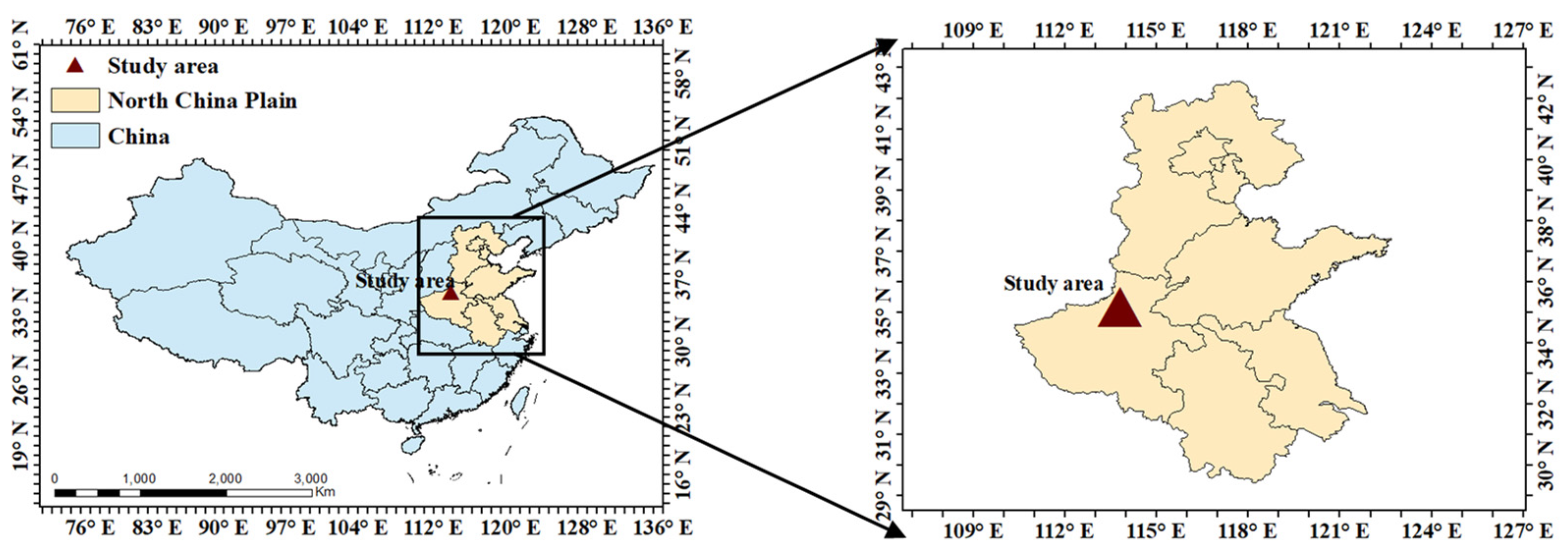
2.1. Description of The Study Area and Experimental Design
2.2. Sampling and Measurements
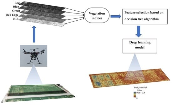
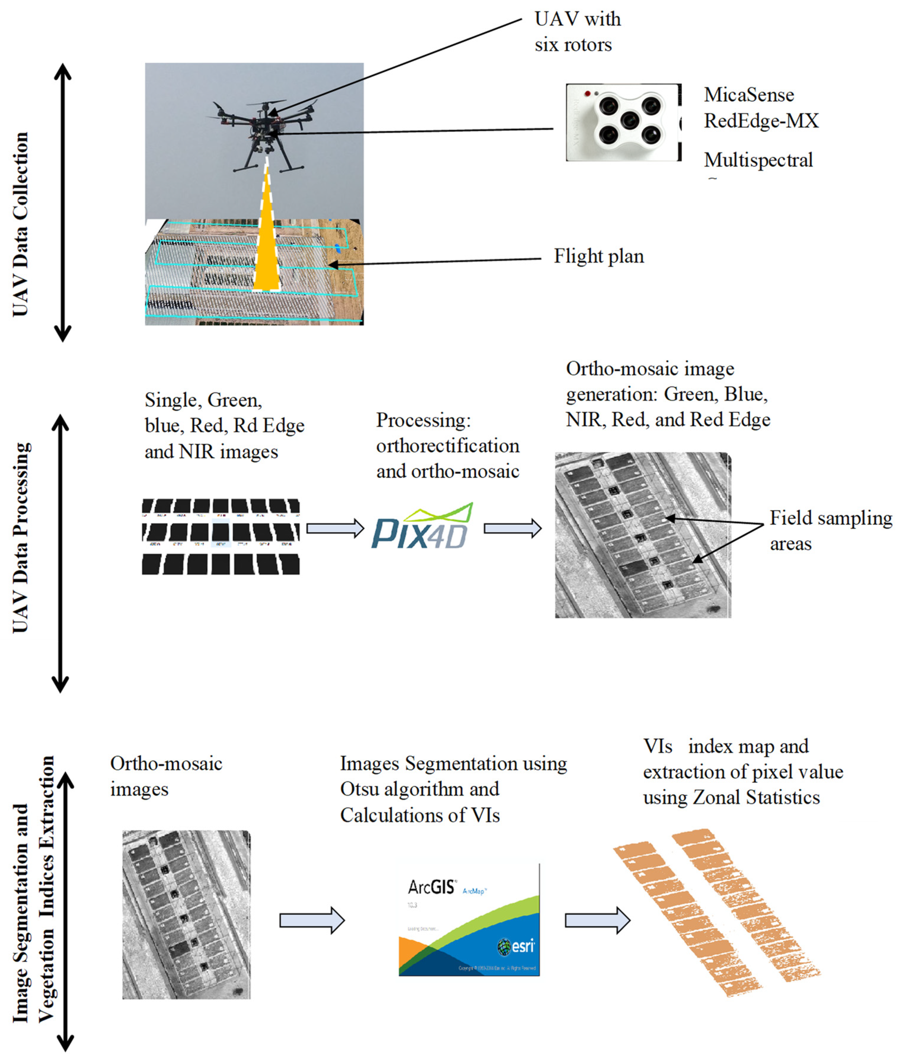
2.3. UAV Data Collection and Processing
2.4. Regression Model Development
2.4.1. Machine Learning for Regression
2.4.2. Multiple Linear Regression
2.4.3. Support Vector Machine
2.4.4. Boosted Regression Tree
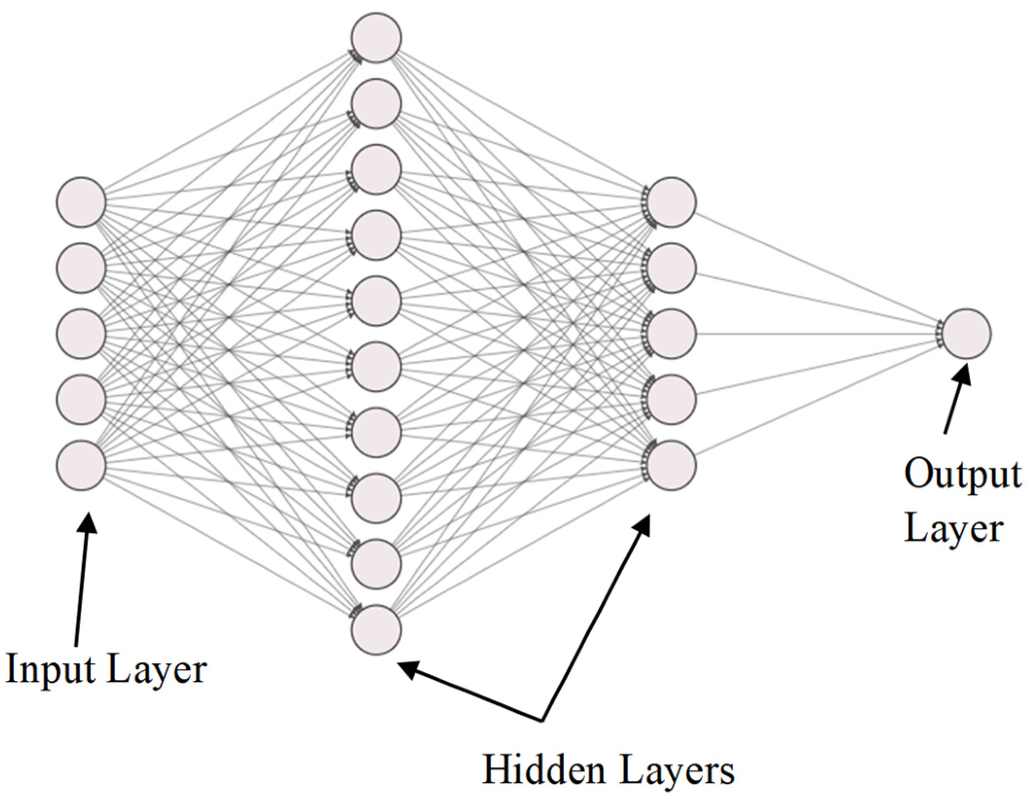
2.4.5. Artificial Neural Network Regression Model
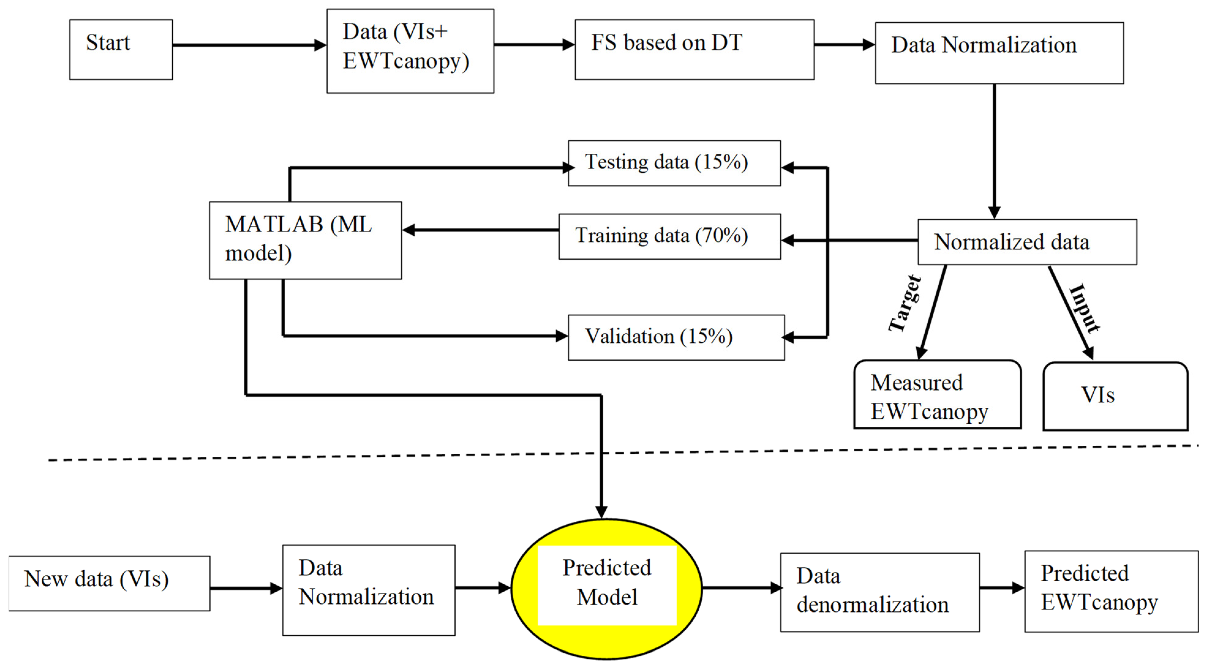
2.4.6. DNN-MLP Model Deployment
2.5. Data Pre-Processing Techniques
2.5.1. Data Normalization
2.5.2. Feature Selection
2.5.3. Model Performance
3. Results
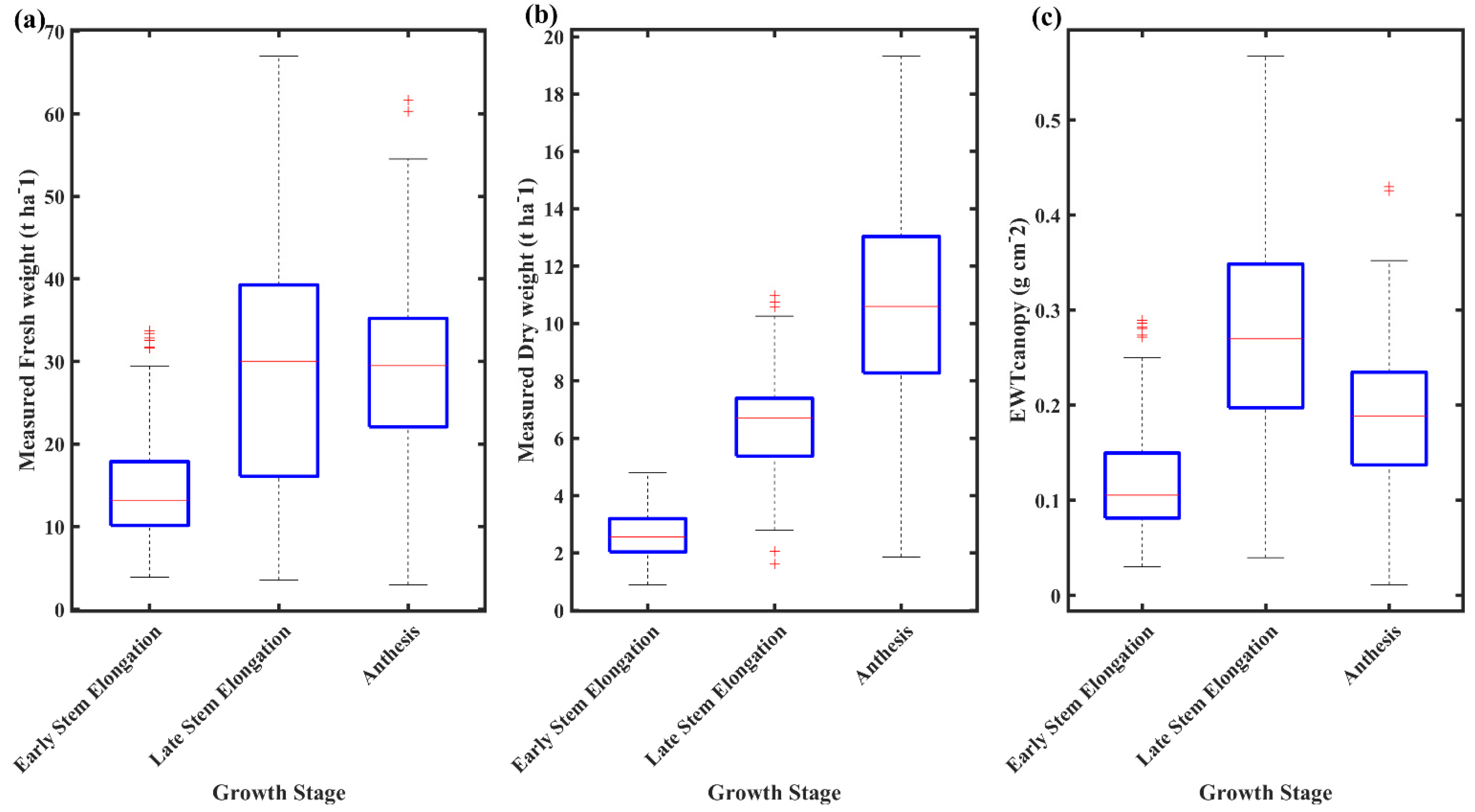
3.1. Dynamic Changes of FW, DW and during the Growth Stage
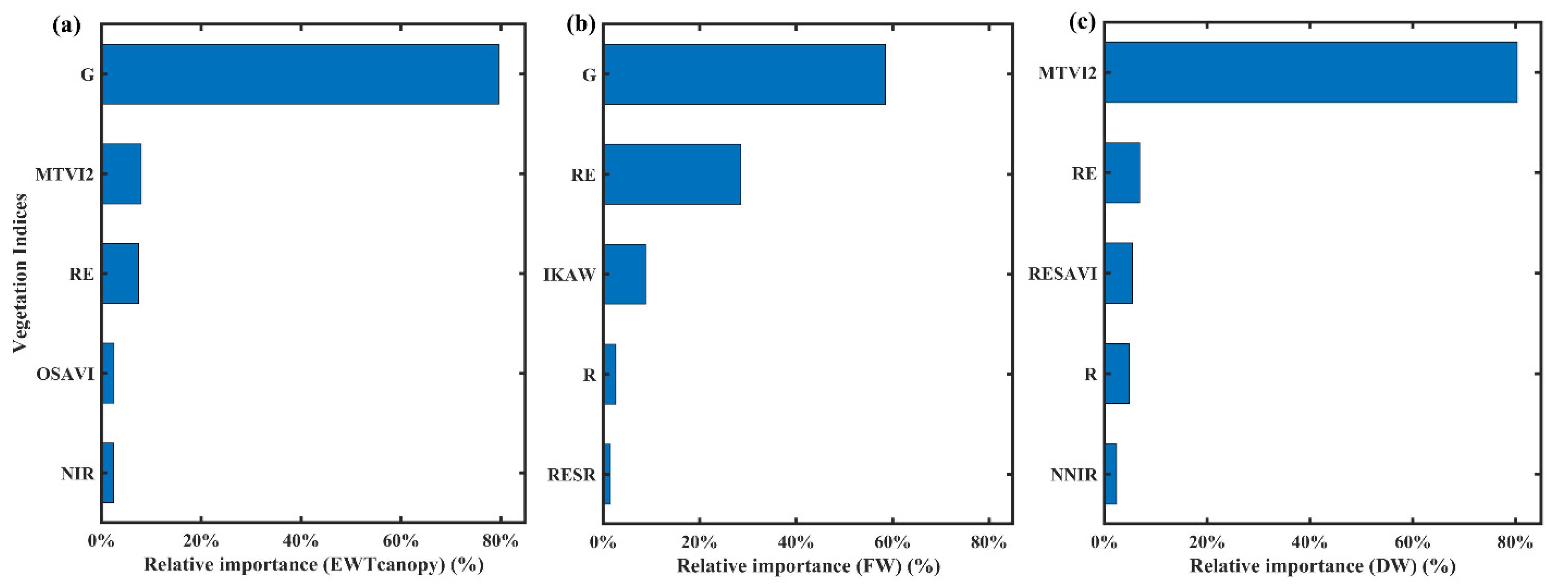
3.2. Variable Inputs’ Effects on FW, DW, and Estimation
3.3. Responses from the Multiple Regression Model
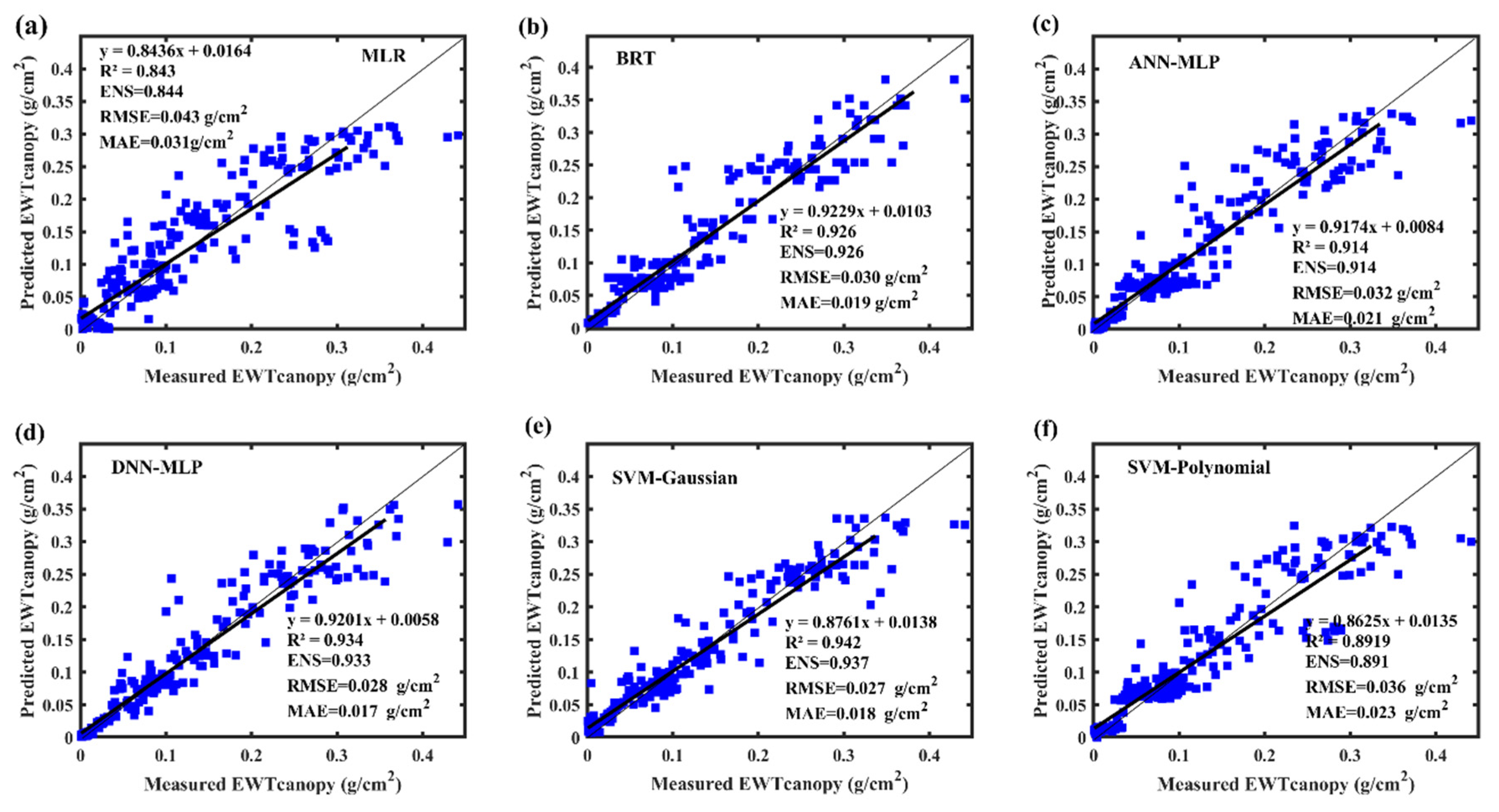
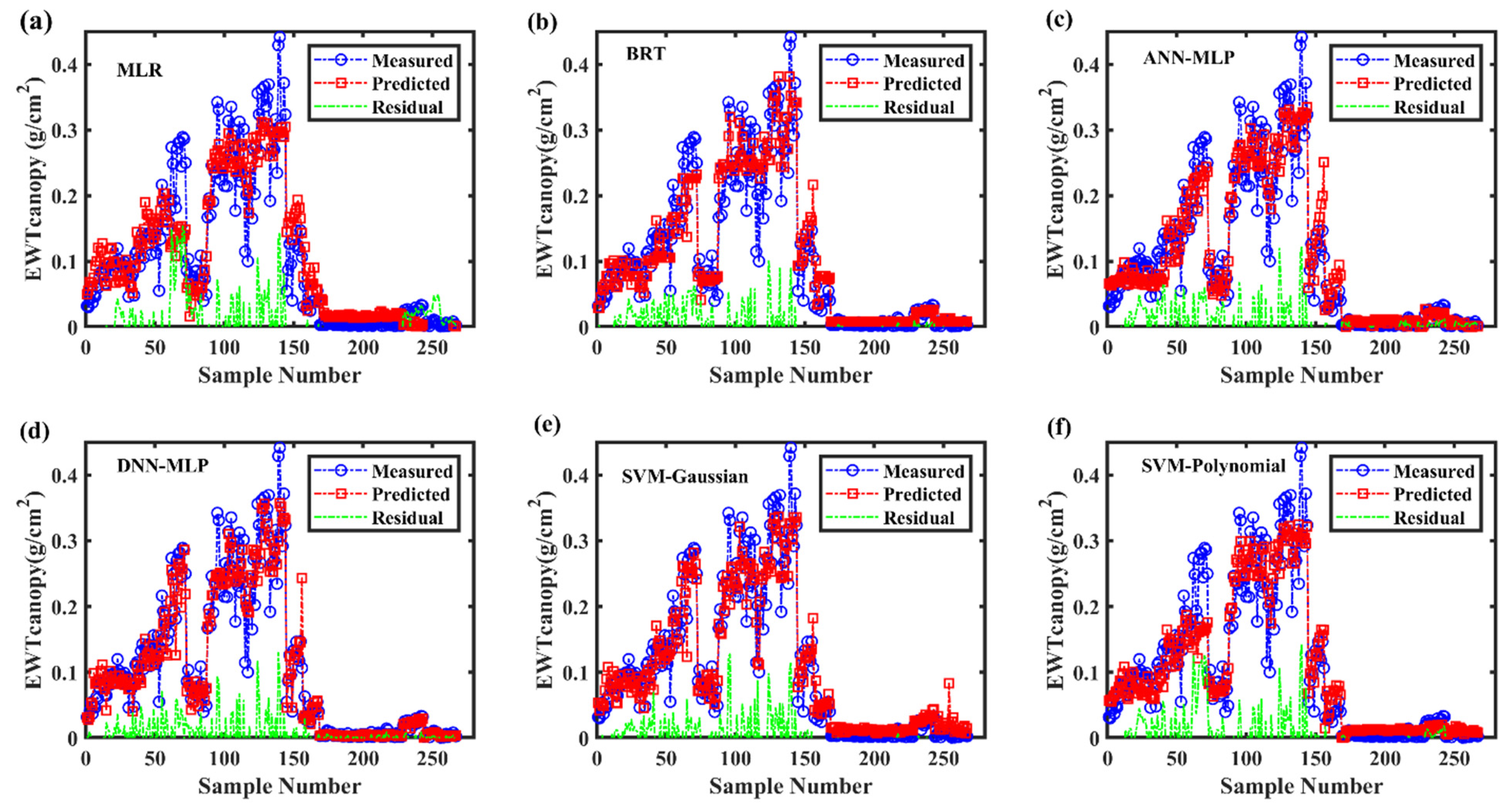
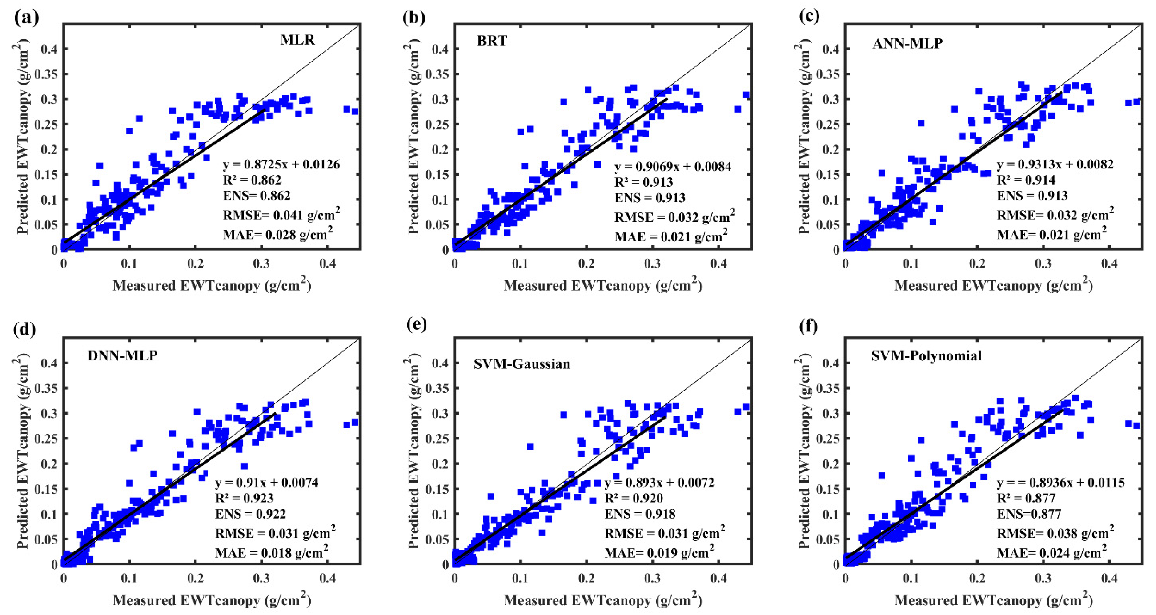
3.4. Modeling Using DNN-MLP, ANN-MLP, BRT, and SVM
3.5. Relationship between Measured and Predicted
3.6. Calculating using Predicted DW and FW
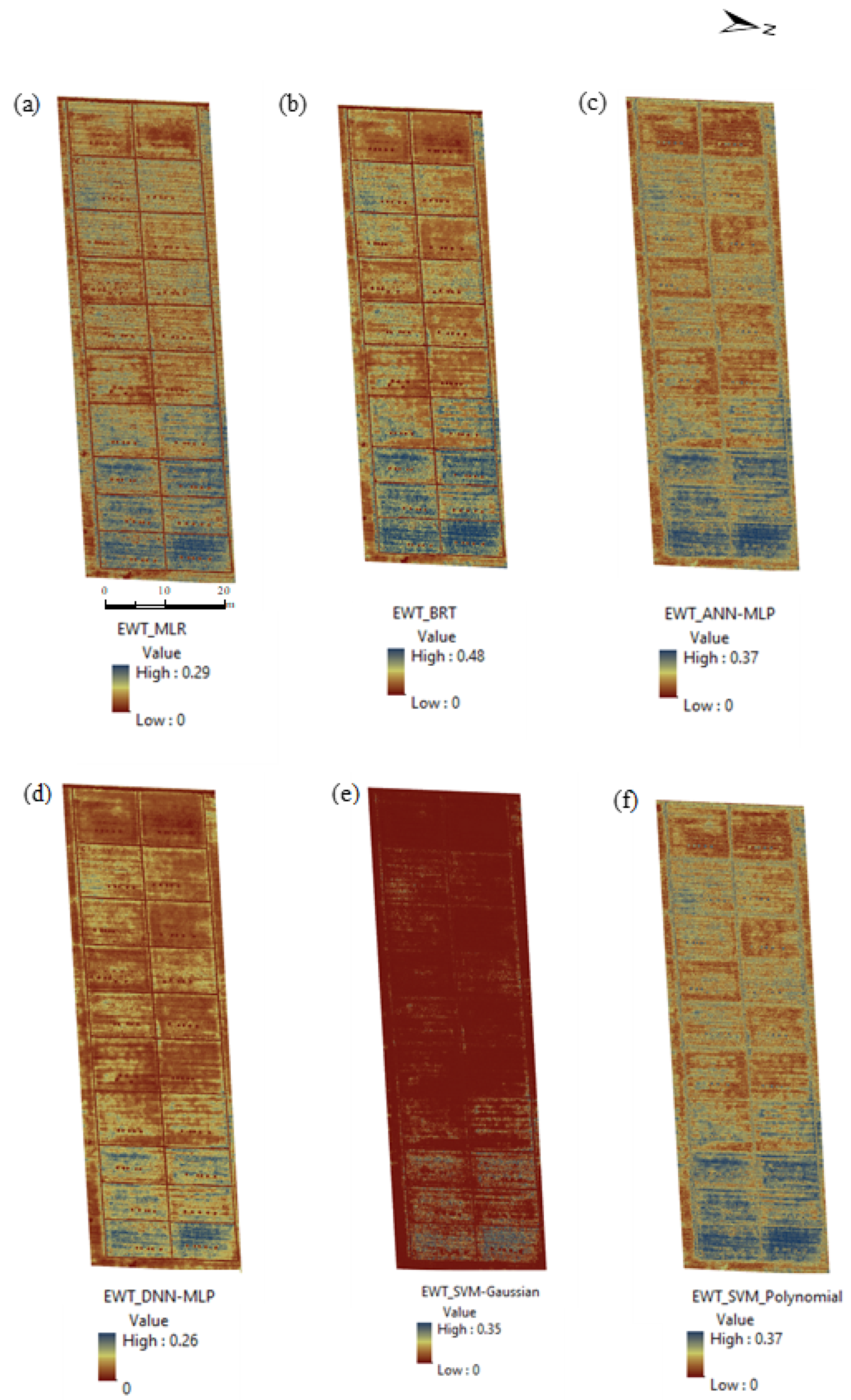
3.7. Model Visualization
4. Discussion
4.1. Dynamic Changes in FW, FW and Ewtcanopy during the Growth Stage
4.2. Performance of the Machine Learning Models
4.3. Feature Selection Methods
4.4. Advantages and Limitations of Machine Learning
5. Conclusions
Author Contributions
Funding
Data Availability Statement
Acknowledgments
Conflicts of Interest
Appendix A

| Vegetations (VIs) | Formulas | References |
|---|---|---|
| Blue Normalized Difference Vegetation Index (BNDV) | (NIR − B)/(NIR + B) | [72] |
| Green Chlorophyll Index (CIg) | NIR/G − 1 | [73] |
| Red Edge Chlorophyll Index (CIre) | NIR/RE − 1 | [25] |
| DATT Index (DATT) | (NIR − RE)/(NIR + R) | [24] |
| Excess Blue Vegetation index (ExB) | (1.4 × B − G)/(G + R + B) | [74] |
| Excess Green minus Excess Red (EXGR) | ExR − ExG | [75] |
| Excess Green index (ExG) | (2 × G − R − B) | [76] |
| Excess Red Vegetation index (ExR) | (1.4 × R − G)/(G + R + B) | [77] |
| Green Difference Vegetation Index (GDVI) | NIR − G | [78] |
| Green Leaf Index (GLI) | (2×G–R–B)/(– R − B) | [79] |
| Green Normalized Difference Vegetation Index (GNDVI) | (NIR − G)/(NIR + G) | [80] |
| Green Optimal Soil Adjusted Vegetation Index (GOSAVI) | (1 + 0.16) (NIR − G)/(NIR + G + 0.16) | [81] |
| Green Re–normalized Different Vegetation Index (GRDVI) | (NIR − G)/SQRT (NIR + G) | [26] |
| Green Ratio Vegetation Index (GRVI) | (G − R)/(G + R) | [82] |
| Green Red Vegetation Index (GRVI_Ratio) | NIR/G | [82] |
| Green Soil Adjusted Vegetation Index (GSAVI) | 1.5× ((NIR − G)/(NIR + G + 0.5)) | [81] |
| Green Wide Dynamic Range Vegetation Index (GWDRVI) | (0.12×NIR − G)/(0.12 × NIR + G) | [83] |
| Kawashima Index (IKAW) | (R − B)/(R + B) | [84] |
| Modified Chlorophyll Absorption in Reflectance Index 1 (MCARI1) | ((NIR − RE) − 0.2 × (NIR − G)) × (NIR/RE) | [85] |
| Modified Chlorophyll Absorption in Reflectance Index 2 (MCARI2) | 1.5 × (2.5 × (NIR − RE) –1.3× (NIR − G))/SQRT (SQ (2 × NIR + 1)) − (6 × NIR − 5 × SQRT(RE) − 0.5) | [86] |
| Modified Chlorophyll Absorption in Reflectance Index 3 (MCARI3) | ((NIR − RE) − 0.2 × (NIR − R))/(NIR/RE) | [26] |
| Modified Chlorophyll Absorption in Reflectance Index 4 (MCARI4) | 1.5 × (2.5 × (NIR − G) –1.3 × (NIR − RE))/SQRT (SQ (2 × NIR + 1)) − (6 × NIR − 5 × SQRT(G) − 0.5) | [26] |
| Modified Double Difference Index Green (MDD) | (NIR − RE) − (RE − G) | [87] |
| Modified Double Difference Index Red (MDD) | (NIR − RE) − (RE − R) | [27] |
| Modified Green Red Vegetation Index (MGRVI) | (SQ(G) − SQ (R))/(SQ(G) + SQ (R)) | [88] |
| Modified Nonlinear Index (MNLI) | 1.5 × (SQ(NIR) − R)/(SQ(NIR) + R + 0.5) | [89] |
| Modified Red Edge Difference Vegetation Index (MREDVI) | RE − R | [26] |
| Modified Red Edge Soil Adjusted Vegetation Index (MRESAVI) | 0.5 × (2 × NIR + 1 − SQRT (SQ (2 × NIR + 1)) − 8 × (NIR − RE)) | [90] |
| Modified Red Edge Transformed Vegetation Index (MRETVI) | 1.2 × (1.2 × (NIR − R) − 2.5 × (RE − R)) | [86] |
| Modified Soil Adjusted Vegetation Index (MSAVI) | 0.5× (2×NIR + 1 − SQRT (SQ (2×NIR + 1) –8× (NIR − G))) | [90] |
| Modified Simple Ratio (MSR) | (NIR/R − 1)/SQRT (NIR/R + 1) | [91] |
| Modified Green Simple Ratio (MSR_G) | (NIR/G − 1)/SQRT (NIR/G + 1) | [91] |
| Modified Red Edge Simple Ratio (MSR_RE) | ((NIR/RE) − 1)/SQRT ((NIR/RE) − 1) | [91] |
| Modified Transformed Chlorophyll Absorption in Reflectance Index (MTCARI) | 3× ((NIR − RE) − 0.2 × (NIR − R) × (NIR/RE)) | [92] |
| Modified Triangular Vegetation Index (MTVI2) | 1.5 × (1.2 × (NIR − G) − (2.5 × R–G))/SQRT (SQ (2 × NIR + 1) − (6 × NIR − 5 × SQRT(R)) − 0.5) | [86] |
| Normalized Difference Red Edge (NDRE) | (NIR − RE)/(NIR + RE) | [93] |
| Normalized Difference Vegetation Index (NDVI) | (NIR − R)/(NIR + R) | [94] |
| Normalized Green Index (NGI) | G/(NIR + RE + G) | [81] |
| Nonlinear Index (NLI) | (SQ(NIR) − R)/(SQ(NIR) + R) | [95] |
| Normalized NIR Index (NNIR) | NIR/(NIR + RE + G) | [81] |
| Normalized Near Infrared Index (NNIRI) | NIR/(NIR + RE + R) | [27] |
| Normalized Red Edge Index (NREI) | RE/(NIR + RE + G) | [81] |
| Normalized Red Edge Index (NREI) | RE/(NIR + RE + R) | [27] |
| Normalized Red Index (NRI) | R/(NIR + RE + R) | [27] |
| Optimized SAVI (OSAVI) | (1 + 0.16) × (NIR − R)/(NIR + R + 0.16) | [96] |
| Renormalized Difference Vegetation Index (RDVI) | (NIR − R)/SQRT (NIR + R) | [97] |
| Red Edge Difference Vegetation Index (REDVI) | NIR − RE | [26] |
| Red Edge Normalized Difference Vegetation Index (RENDVI) | (RE − R)/(RE + R) | [98] |
| Red Edge Optimal Soil Adjusted Vegetation Index (REOSAVI) | (1 + 0.16) × (NIR − RE)/(NIR + RE + 0.16) | [96] |
| Red Edge Renormalized Different Vegetation Index (RERDVI) | (NIR − RE)/SQRT (NIR + RE) | [26] |
| Red Edge Ratio Vegetation Index (RERVI) | NIR/RE | [99] |
| Red Edge Soil Adjusted Vegetation Index (RESAVI) | 1.5× ((NIR − RE)/(NIR + RE + 0.5)) | [81] |
| Red Edge Simple Ratio (RESR) | RE/R | [100] |
| Red Edge Transformed Vegetation Index (RETVI) | 0.5× (120× (NIR − R) – 200 × (RE − R)) | [91] |
| Optimized Red Edge Vegetation Index (REVIopt) | 100 × (Ln (NIR) − Ln (RE)) | [101] |
| Red Edge Wide Dynamic Range Vegetation Index (REWDRVI) | (0.12×NIR − RE)/(0.12 × NIR + RE) | [83] |
| Red Green Blue Vegetation Index (RGBVI) | (SQ(G) − (B × R))/(SQ(G) + (B × R)) | [88] |
| Ratio Vegetation Index (RVI) | NIR/R | [102] |
| Soil–Adjusted Vegetation Index (SAVI) | 1.5× (NIR − R)/(NIR + R + 0.5) | [103] |
| Transformed Normalized Vegetation Index (TNDVI) | SQRT ((NIR − R)/(NIR + R) + 0.5) | [104] |
| Optimal Vegetation Index (VIopt) | 1.45×(SQ(NIR) + 1)/(R + 0.45) | [101] |
| Wide Dynamic Range Vegetation Index (WDRVI) | (0.12×NIR − R)/(0.12 × NIR + R) | [83] |
| Vegetation Indices/Bands | Mean ± SD | Min. | Max. | Vegetation Indices/Bands | Mean ± SD | Min. | Max. |
|---|---|---|---|---|---|---|---|
| B | 0.03 ± 0.02 | 0.08 | 0.01 | MSR_RE | 1.25 ± 0.55 | 2.12 | 0.51 |
| BNDV | 0.82 ± 0.11 | 0.95 | 0.62 | MTCARI | 0.04 ± 0.16 | 0.23 | –0.39 |
| Cig | 6.48 ± 4.33 | 14.99 | 1.59 | MTVI2 | 0.34 ± 0.35 | 0.84 | –0.17 |
| CIre | 1.88 ± 1.41 | 4.51 | 0.26 | NDRE | 0.41 ± 0.2 | 0.69 | 0.11 |
| DATT | 0.48 ± 0.25 | 0.8 | 0.12 | NDVI | 0.64 ± 0.29 | 0.95 | 0.2 |
| ExB | –0.13 ± 0.07 | –0.05 | –0.26 | NGI | 0.11 ± 0.04 | 0.18 | 0.05 |
| ExG | 0.01 ± 0.04 | 0.06 | –0.07 | NIR | 0.38 ± 0.08 | 0.53 | 0.23 |
| ExGR | 0.09 ± 0.31 | 0.55 | –0.33 | NLI | 0.31 ± 0.5 | 0.91 | –0.46 |
| ExR | 0.1 ± 0.28 | 0.49 | –0.29 | NNIR | 0.63 ± 0.12 | 0.8 | 0.46 |
| G | 0.07 ± 0.03 | 0.14 | 0.03 | NNIRI | 0.62 ± 0.15 | 0.83 | 0.41 |
| GDVI | 0.31 ± 0.1 | 0.48 | 0.14 | NREI_G | 0.26 ± 0.08 | 0.37 | 0.15 |
| GLI | –0.57 ± 0.62 | 0.21 | –1.68 | NREI_R | 0.25 ± 0.06 | 0.32 | 0.15 |
| GNDVI | 0.69 ± 0.15 | 0.88 | 0.44 | NRI | 0.13 ± 0.1 | 0.27 | 0.02 |
| GOSAVI | 0.46 ± 0.12 | 0.65 | 0.25 | OSAVI | 0.55 ± 0.25 | 0.85 | 0.18 |
| GRDVI | 0.59 ± 0.14 | 0.79 | 0.34 | R | 0.08 ± 0.07 | 0.27 | 0.01 |
| GRVI | 0.07 ± 0.28 | 0.47 | –0.32 | RDVI | 0.43 ± 0.2 | 0.69 | 0.14 |
| GRVI_Ratio | 7.48 ± 4.33 | 15.99 | 2.59 | RE | 0.16 ± 0.05 | 0.33 | 0.09 |
| GSAVI | 0.49 ± 0.13 | 0.69 | 0.26 | REDVI | 0.23 ± 0.12 | 0.42 | 0.06 |
| GWDRVI | –0.14 ± 0.28 | 0.31 | –0.53 | RENDVI | 0.44 ± 0.26 | 0.78 | 0.09 |
| IKAW | 0.25 ± 0.21 | 0.54 | –0.06 | REOSAVI | 0.36 ± 0.19 | 0.63 | 0.1 |
| MCARI1 | 0.61 ± 0.55 | 1.77 | 0.03 | RERDVI | 0.41 ± 0.32 | 1.36 | 0.09 |
| MCARI2 | 0.29 ± 0.6 | 1.16 | –0.75 | RERVI | 2.77 ± 1.57 | 5.51 | 0.09 |
| MCARI3 | 0.05 ± 0.01 | 0.08 | 0.03 | RESAVI | 0.42 ± 0.29 | 1.23 | 0.09 |
| MCARI4 | –0.1 ± 0.64 | 0.89 | –1.21 | RESR | 3.63 ± 2.27 | 8.1 | 1.19 |
| MDD_G | 0.13 ± 0.14 | 0.36 | –0.09 | RETVI | 10.35 ± 6.55 | 21.96 | 2.01 |
| MDD_R | 0.15 ± 0.1 | 0.34 | 0.02 | REVIopt | 92.05 ± 51.11 | 170.3 | 22.94 |
| MGRVI | 0.12 ± 0.51 | 0.77 | –0.58 | REWDRVI | –0.51 ± 0.18 | –0.21 | –0.74 |
| MNLI | 0.14 ± 0.24 | 0.49 | –0.2 | RGBVI | 0.36 ± 0.3 | 0.75 | –0.06 |
| MREDVI | 0.07 ± 0.02 | 0.12 | 0.03 | RVI | 13.69 ± 13.08 | 44.02 | 1.5 |
| MRESAVI | –0.89 ± 0.48 | –0.22 | –1.69 | SAVI | 0.46 ± 0.21 | 0.73 | 0.15 |
| MRETVI | 0.2 ± 0.15 | 0.48 | 0.03 | TNDVI | 1.06 ± 0.14 | 1.21 | 0.84 |
| MSAVI | 0.49 ± 0.16 | 0.76 | 0.23 | VIopt | 3.21 ± 0.53 | 3.98 | 2.39 |
| MSR | 2.65 ± 2.01 | 6.38 | 0.32 | WDRVI | –0.06 ± 0.5 | 0.67 | –0.7 |
| MSR_G | 2.04 ± 0.92 | 3.63 | 0.84 |
References
- Li, L.; Cheng, Y.-B.; Ustin, S.; Hu, X.-T.; Riaño, D. Retrieval of vegetation equivalent water thickness from reflectance using genetic algorithm (GA)-partial least squares (PLS) regression. Adv. Space Res. 2008, 41, 1755–1763. [Google Scholar] [CrossRef]
- Penuelas, J.; Filella, I.; Biel, C.; Serrano, L.; Savé, R. The reflectance at the 950-970 nm region as an indicator of plant water staus. Int. J. Remote Sens. 1993, 14, 1887–1905. [Google Scholar] [CrossRef]
- Hunt, E.R.; Rock, B.N. Detection of Changes in Leaf Water Content Using Near-and Middle-Infrared Reflectances. Remote Sens. Environ. 1989, 30, 43–54. [Google Scholar] [CrossRef]
- Jackson, T.J.; Chen, D.; Cosh, M.; Li, F.; Anderson, M.; Walthall, C.; Doriaswamy, P.; Hunt, E.B. Vegetation water content mapping using Landsat data derived normalized difference water index for corn and soybeans. Remote Sens. Environ. 2004, 92, 427–435. [Google Scholar] [CrossRef]
- Zhang, Z.; Tang, B.H.; Li, Z.L. Retrieval of leaf water content from remotely sensed data using a vegetation index model constructed with shortwave infrared reflectances. Int. J. Remote Sens. 2019, 40, 2313–2323. [Google Scholar] [CrossRef]
- Gao, B.-C.; Goetzt, A.F.H. Retrieval of equivalent water thickness and information related to biochemical components of vegetation canopies from AVIRIS data. Remote Sens. Environ. 1995, 52, 155–162. [Google Scholar] [CrossRef]
- Zhang, F.; Zhou, G. Estimation of vegetation water content using hyperspectral vegetation indices: A comparison of crop water indicators in response to water stress treatments for summer maize. BMC Ecol. 2019, 19, 18. [Google Scholar] [CrossRef] [Green Version]
- Zhang, L.; Niu, Y.; Zhang, H.; Han, W.; Li, G.; Tang, J.; Peng, X. Maize Canopy Temperature Extracted From UAV Thermal and RGB Imagery and Its Application in Water Stress Monitoring. Front. Plant Sci. 2019, 10, 1270. [Google Scholar] [CrossRef]
- Hassan, M.A.; Yang, M.; Fu, L.; Rasheed, A.; Zheng, B. Accuracy assessment of plant height using an unmanned aerial vehicle for quantitative genomic analysis in bread wheat. Plant Methods 2019, 15, 1–12. [Google Scholar] [CrossRef] [Green Version]
- Shafian, S.; Rajan, N.; Schnell, R.; Bagavathiannan, M.; Valasek, J.; Shi, Y.; Olsenholler, J. Unmanned aerial systems-based remote sensing for monitoring sorghum growth and development. PLoS ONE 2018, 15, e0196605. [Google Scholar] [CrossRef] [PubMed] [Green Version]
- Xia, X.; Xiao, Y.; He, Z. Time-Series Multispectral Indices from Unmanned Aerial Vehicle Imagery Reveal Senescence Rate in Bread Wheat. Remote Sens. 2018, 10, 809. [Google Scholar] [CrossRef] [Green Version]
- Smigaj, M.; Gaulton, R.; Suárez, J.C.; Barr, S.L. Forest Ecology and Management Canopy temperature from an Unmanned Aerial Vehicle as an indicator of tree stress associated with red band needle blight severity. For. Ecol. Manag. 2019, 433, 699–708. [Google Scholar] [CrossRef]
- Poblete, T.; Ortega-far, S.; Bardeen, M. Artificial Neural Network to Predict Vine Water Status Spatial Variability Using Multispectral Information Obtained from an Unmanned Aerial Vehicle (UAV). Sensors 2017, 17, 2488. [Google Scholar] [CrossRef] [PubMed] [Green Version]
- Gao, B.-c. NDWI—A normalized difference water index for remote sensing of vegetation liquid water from space. Remote Sens. Environ. 1996, 58, 257–266. [Google Scholar] [CrossRef]
- Ceccato, P.; Flasse, S.; Tarantola, S.; Jacquemoud, S.; Grégoire, J.M. Detecting vegetation leaf water content using reflectance in the optical domain. Remote Sens. Environ. 2001, 77, 22–33. [Google Scholar] [CrossRef]
- Mobasheri, M.R.; Fatemi, S.B. Leaf Equivalent Water Thickness assessment using reflectance at optimum wavelengths. Theor. Exp. Plant Physiol. 2013, 25, 196–202. [Google Scholar] [CrossRef] [Green Version]
- Ceccato, P.; Gobron, N.; Flasse, S.; Pinty, B.; Tarantola, S. Designing a spectral index to estimate vegetation water content from remote sensing data: Part 2. Validation and applications. Remote Sens. Environ. 2002, 82, 198–207. [Google Scholar] [CrossRef]
- Sibanda, M.; Mutanga, O.; Dube, T.; Mothapo, M.C.; Mafongoya, P.L. Remote sensing equivalent water thickness of grass treated with different fertiliser regimes using resample HyspIRI and EnMAP data. Phys. Chem. Earth Parts A/B/C 2019, 112, 246–254. [Google Scholar] [CrossRef]
- Tucker, C.J. Remote Sensing of Leaf Water Content in the Near Irdrared. Remote Sens. Environ. 1980, 10, 23–32. [Google Scholar] [CrossRef]
- Liu, S.; Peng, Y.; Du, W.; Le, Y.; Li, L. Remote estimation of leaf and canopy water content in winter wheat with different vertical distribution of water-related properties. Remote Sens. 2015, 7, 4626–4650. [Google Scholar] [CrossRef] [Green Version]
- Wocher, M.; Berger, K.; Danner, M.; Mauser, W.; Hank, T. Physically-Based Retrieval of Canopy Equivalent Water Thickness Using Hyperspectral Data. Remote Sens. 2018, 10, 1924. [Google Scholar] [CrossRef] [Green Version]
- Dennison, P.E.; Roberts, D.A.; Thorgusen, S.R.; Regelbrugge, J.C.; Weise, D.; Lee, C. Modeling seasonal changes in live fuel moisture and equivalent water thickness using a cumulative water balance index. Remote Sens. Environ. 2003, 88, 442–452. [Google Scholar] [CrossRef]
- Yao, X.; Jia, W.; Si, H.; Guo, Z.; Tian, Y.; Liu, X.; Cao, W.; Zhu, Y. Exploring novel bands and key index for evaluating leaf equivalent water thickness in wheat using hyperspectra influenced by nitrogen. PLoS ONE 2014, 9, e96352. [Google Scholar] [CrossRef] [PubMed]
- Datt, B. Visible/near infrared reflectance and chlorophyll content in Eucalyptus leaves. Int. J. Remote Sens. 1999, 20, 2741–2759. [Google Scholar] [CrossRef]
- Gitelson, A.A.; Gritz, Y.; Merzlyak, M.N. Relationships between leaf chlorophyll content and spectral reflectance and algorithms for non-destructive chlorophyll assessment in higher plant leaves. J. Plant Physiol. 2003, 160, 271–280. [Google Scholar] [CrossRef]
- Cao, Q.; Miao, Y.; Wang, H.; Huang, S.; Cheng, S.; Khosla, R.; Jiang, R. Non-destructive estimation of rice plant nitrogen status with Crop Circle multispectral active canopy sensor. Field Crop. Res. 2013, 154, 133–144. [Google Scholar] [CrossRef]
- Lu, J.; Miao, Y.; Shi, W.; Li, J.; Yuan, F. Evaluating different approaches to non-destructive nitrogen status diagnosis of rice using portable RapidSCAN active canopy sensor. Sci. Rep. 2017, 7, 14073. [Google Scholar] [CrossRef] [PubMed]
- Thornton, B.; Lemaire, G.; Millard, P.; Duff, E.I. Relationships Between Nitrogen and Water Concentration in Shoot Tissue of Molinia caerulea During Shoot Development. Ann. Bot. 1999, 83, 631–636. [Google Scholar] [CrossRef] [Green Version]
- Sims, D.A.; Gamon, J.A. Estimation of vegetation water content and photosynthetic tissue area from spectral reflectance: A comparison of indices based on liquid water and chlorophyll absorption features. Remote Sens. Environ. 2003, 84, 526–537. [Google Scholar] [CrossRef]
- Dawson, T.P.; Curran, P.J. The biochemical decomposition of slash pine needles from reflectance spectra using neural networks. Int. J. Remote Sens. 2010, 19, 37–41. [Google Scholar] [CrossRef]
- Ustin, S.L.; Roberts, D.A.; Pinzo, J.; Jacquemoud, S.; Gardner, M.; Scheer, G.; Castan, C.M. Estimating Canopy Water Content of Chaparral Shrubs Using Optical Methods. Remote Sens. Environ. 1996, 4257, 280–291. [Google Scholar] [CrossRef]
- Mia, M.; Dhar, N.R. Prediction of surface roughness in hard turning under high pressure coolant using Artificial Neural Network. Meas. J. Int. Meas. Confed. 2016, 92, 464–474. [Google Scholar] [CrossRef]
- Khan, M.S.; Semwal, M.; Sharma, A.; Verma, R.K. An artificial neural network model for estimating Mentha crop biomass yield using Landsat 8 OLI. Precis. Agric. 2020, 21, 18–33. [Google Scholar] [CrossRef]
- Jin, X.; Li, Z.; Feng, H.; Ren, Z.; Li, S. Deep neural network algorithm for estimating maize biomass based on simulated Sentinel 2A vegetation indices and leaf area index. Crop J. 2020, 8, 87–97. [Google Scholar] [CrossRef]
- Veenadhari, S.; Misra, B.; Singh, C.D. Machine learning approach for forecasting crop yield based on climatic parameters. In Proceedings of the 2014 International Conference on Computer Communication and Informatics, Coimbatore, India, 3–5 January 2014. [Google Scholar] [CrossRef]
- Worland, S.C.; Farmer, W.H.; Kiang, J.E. Improving predictions of hydrological low-flow indices in ungaged basins using machine learning. Environ. Model. Softw. 2018, 101, 169–182. [Google Scholar] [CrossRef]
- Nguyen, V.T.; Constant, T.; Kerautret, B.; Debled-Rennesson, I.; Colin, F. A machine-learning approach for classifying defects on tree trunks using terrestrial LiDAR. Comput. Electron. Agric. 2020, 171, 105332. [Google Scholar] [CrossRef]
- Khan, A.; Sohail, A.; Zahoora, U.; Qureshi, A.S. A Survey of the Recent Architectures of Deep Convolutional Neural Networks 1 Introduction. Artif. Intell. Rev. 2020, 53, 5455–5516. [Google Scholar] [CrossRef] [Green Version]
- Zha, H.; Miao, Y.; Wang, T.; Li, Y.; Zhang, J.; Sun, W. Sensing-Based Rice Nitrogen Nutrition Index Prediction with Machine Learning. Remote Sens. 2020, 12, 215. [Google Scholar] [CrossRef] [Green Version]
- Li, S.; Ding, X.; Kuang, Q.; SyedTahir, A.-U.-K.; Cheng, T.; Xiaojun, L.; Yongchao, T.; Zhu, Y.; Cao, W.; Cao, Q. Potential of UAV-based active sensing for monitoring rice leaf nitrogen status. Front. Plant Sci. 2018, 9, 1834. [Google Scholar] [CrossRef] [PubMed] [Green Version]
- Colombo, R.; Meroni, M.; Marchesi, A.; Busetto, L.; Rossini, M.; Giardino, C.; Panigada, C. Estimation of leaf and canopy water content in poplar plantations by means of hyperspectral indices and inverse modeling. Remote Sens. Environ. 2008, 112, 1820–1834. [Google Scholar] [CrossRef]
- Wang, N.; Wang, Y.; Er, M.J. Review on deep learning techniques for marine object recognition: Architectures and algorithms. Control Eng. Pract. 2020, 1–18. [Google Scholar] [CrossRef]
- Batlles, F.J.; Tovar-pescador, J.; Lo, G. Selection of input parameters to model direct solar irradiance by using artificial neural networks. Energy 2005, 30, 1675–1684. [Google Scholar] [CrossRef]
- Venkatesh, B.; Anuradha, J. A Review of Feature Selection and Its Methods. Bulg. Acad. Sci. Cybern. 2019, 19, 3–26. [Google Scholar] [CrossRef] [Green Version]
- Khaki, S.; Wang, L. Crop Yield Prediction Using Deep Neural Networks. Front. Plant Sci. 2019, 10, 621. [Google Scholar] [CrossRef] [Green Version]
- Ruggieri, S. Complete search for feature selection in decision trees. J. Mach. Learn. Res. 2019, 20, 104. [Google Scholar]
- Romalt, A.A.; Kumar, R.M.S. An Analysis on Feature Selection Methods, Clustering and Classification used in Heart Disease Prediction—A Machine Learning Approach. J. Crit. Rev. 2020, 7, 138–142. [Google Scholar] [CrossRef]
- Zhou, H.F.; Zhang, J.W.; Zhou, Y.Q.; Guo, X.J.; Ma, Y.M. A feature selection algorithm of decision tree based on feature weight. Expert Syst. Appl. 2021, 164, 113842. [Google Scholar] [CrossRef]
- Otsu, N. A threshold Selection Method from Gray-Level Histograms. IIEEE Trans. Syst. Man Cybern. 1979, 9, 62–66. [Google Scholar] [CrossRef] [Green Version]
- Corti, M.; Marino, P.; Cavalli, D.; Cabassi, G. Hyperspectral imaging of spinach canopy under combined water and nitrogen stress to estimate biomass, water, and nitrogen content. Biosyst. Eng. 2017, 158, 38–50. [Google Scholar] [CrossRef]
- Boser, B.E.; Laboratories, T.B.; Guyon, I.M.; Laboratories, T.B.; Vapnik, V.N. A Training Algorithm for Optimal Margin Classi ers. In Proceedings of the Fifth Annual Workshop on Computational Learning Theory, Pittsburgh, PA, USA, 1 July 1992; pp. 144–152. [Google Scholar] [CrossRef]
- Fan, J.; Zheng, J.; Wu, L.; Zhang, F. Estimation of daily maize transpiration using support vector machines, extreme gradient boosting, artificial and deep neural networks models. Agric. Water Manag. 2021, 245, 106547. [Google Scholar] [CrossRef]
- Durbha, S.S.; King, R.L.; Younan, N.H. Support vector machines regression for retrieval of leaf area index from multiangle imaging spectroradiometer. Remote Sens. Environ. 2007, 107, 348–361. [Google Scholar] [CrossRef]
- Shadkani, S.; Abbaspour, A.; Samadianfard, S.; Hashemi, S.; Mosavi, A.; Band, S.S. Comparative study of multilayer perceptron-stochastic gradient descent and gradient boosted trees for predicting daily suspended sediment load: The case study of the Mississippi River, U.S. Int. J. Sediment Res. 2020, 36, 512–523. [Google Scholar] [CrossRef]
- Zhang, L.; Traore, S.; Ge, J.; Li, Y.; Wang, S.; Zhu, G.; Cui, Y.; Fipps, G. Using boosted tree regression and artificial neural networks to forecast upland rice yield under climate change in Sahel. Comput. Electron. Agric. 2019, 166, 105031. [Google Scholar] [CrossRef]
- Puri, P.; Comfere, N.; Drage, L.A.; Shamim, H.; Bezalel, S.A.; Pittelkow, M.R.; Davis, M.D.P.; Wang, M.; Mangold, A.R.; Tollefson, M.M.; et al. Deep learning for dermatologists: Part II. Current applications. J. Am. Acad. Dermatol. 2020. [Google Scholar] [CrossRef]
- Singh, P.; Dash, M.; Mittal, P.; Nandi, S.; Nandi, S. Misbehavior Detection in C-ITS Using Deep Learning Approach. Adv. Intell. Syst. Comput. Intell. Syst. Des. Appl. 2020, 641–652. [Google Scholar] [CrossRef]
- Yekkala, I.; Dixit, S. Prediction of Heart Disease Using Random Forest and Rough Set Based Feature Selection. Int. J. Big Data Anal. Healthc. 2018, 3, 1–12. [Google Scholar] [CrossRef] [Green Version]
- Nash, J.E.; Sutcliffe, J. V River flow forecasting through conceptual models part I—A discussion of principles. J. Hydrol. 1970, 10, 282–290. [Google Scholar] [CrossRef]
- Gong, L.; Yu, M.; Jiang, S.; Cutsuridis, V.; Pearson, S. Deep Learning Based Prediction on Greenhouse Crop Yield Combined TCN and RNN. Sensor 2021, 21, 4537. [Google Scholar] [CrossRef]
- Huang, T.; Wang, S.; Sharma, A. Highway crash detection and risk estimation using deep learning. Accid. Anal. Prev. 2020, 135, 105392. [Google Scholar] [CrossRef]
- Kim, A.; Yang, Y.; Lessmann, S.; Ma, T.; Sung, M.C.; Johnson, J.E.V. Can deep learning predict risky retail investors? A case study in financial risk behavior forecasting. Eur. J. Oper. Res. 2020, 283, 217–234. [Google Scholar] [CrossRef] [Green Version]
- Shao, M.; Wang, X.; Bu, Z.; Chen, X.; Wang, Y. Prediction of energy consumption in hotel buildings via support vector machines. Sustain. Cities Soc. 2020, 57, 102128. [Google Scholar] [CrossRef]
- Haq, A.U.; Zeb, A.; Lei, Z.; Zhang, D. Forecasting daily stock trend using multi-filter feature selection and deep learning. Expert Syst. Appl. 2021, 168, 114444. [Google Scholar] [CrossRef]
- Al-Harbi, O. A Comparative Study of Feature Selection Methods for Dialectal Arabic Sentiment Classification Using Support Vector Machine. arXiv 2019, arXiv:1902.06242. [Google Scholar]
- Rao, H.; Shi, X.; Rodrigue, A.K.; Feng, J.; Xia, Y.; Elhoseny, M.; Yuan, X.; Gu, L. Feature selection based on artificial bee colony and gradient boosting decision tree. Appl. Soft Comput. J. 2019, 74, 634–642. [Google Scholar] [CrossRef]
- Elarab, M. The Application of Unmanned Aerial Vehicle to Precision Agriculture: Chlorophyll, Nitrogen, and Evapotranspiration Estimation; Utah State University: Logan, UT, USA, 2014. [Google Scholar]
- Berni, J.A.J.; Member, S.; Zarco-tejada, P.J.; Suárez, L.; Fereres, E. Thermal and Narrowband Multispectral Remote Sensing for Vegetation Monitoring From an Unmanned Aerial Vehicle. IEEE Trans. Geosci. Remote Sens. 2009, 47, 722–738. [Google Scholar] [CrossRef] [Green Version]
- Sánchez-Sastre, L.F.; Alte da Veiga, N.M.S.; Ruiz-Potosme, N.M.; Carrión-Prieto, P.; Marcos-Robles, J.L.; Navas-Gracia, L.M.; Martín-Ramos, P. Assessment of RGB Vegetation Indices to Estimate Chlorophyll Content in Sugar Beet Leaves in the Final Cultivation Stage. AgriEngineering 2019, 2, 128–149. [Google Scholar] [CrossRef] [Green Version]
- Tsouros, D.C.; Bibi, S.; Sarigiannidis, P.G. A Review on UAV-Based Applications for Precision Agriculture. Information 2019, 10, 349. [Google Scholar] [CrossRef] [Green Version]
- Oniga, V.; Breaban, A.; Statescu, F. Determining the Optimum Number of Ground Control Points for Obtaining High Precision Results Based on UAS Images. Proceedings 2018, 2, 165. [Google Scholar] [CrossRef] [Green Version]
- Wang, F.; Huang, J.; Tang, Y.; Wang, X. New Vegetation Index and Its Application in Estimating Leaf Area Index of Rice. Chinese J. Rice Sci. 2007, 14, 195–203. [Google Scholar] [CrossRef]
- Gitelson, A.A.; Vina, A.; Ciganda, V.; Rundquist, D.C.; Arkebauer, T.J. Remote estimation of canopy chlorophyll content in crops. Geophys. Res. Lett. 2005, 32, 4–7. [Google Scholar] [CrossRef] [Green Version]
- Mao, W.; Student, P.D.; Wang, Y.; Wang, Y. Real-time Detection of Between-row Weeds Using Machine Vision. Soc. Eng. Agric. Food Biol. Syst. 2003, 031004. [Google Scholar] [CrossRef]
- Neto, J.C. A Combined Statistical-Soft Computing Approach for Classification and Mapping Weed Species in Minimum-Tillage Systems; ProQuest Dissertations: Lincoln, NE, USA, 2004. [Google Scholar]
- Woebbecke, D.M.; Meyer, G.E.; Von Bargen, K.; Mortensen, D.A. Color Indices for Weed Identification Under Various Soil, Residue, and Lighting Conditions. Am. Soc. Agric. Eng. 1995, 3, 259–269. [Google Scholar] [CrossRef]
- Meyer, G.E.; Neto, J.C. Verification of color vegetation indices for automated crop imaging applications. Comput. Electron. Agric. 2008, 3, 282–293. [Google Scholar] [CrossRef]
- Tucker, C.J. Red and Photographic Infrared linear Combinations for Monitoring Vegetation. Remote Sens. Environ. 1979, 8, 127–150. [Google Scholar] [CrossRef] [Green Version]
- Louhaichi, M.; Borman, M.M.; Johnson, D.E. Spatially Located Platform and Aerial Photography for Documentation of Grazing Impacts on Wheat. Geocarto Int. 2001, 16, 65–70. [Google Scholar] [CrossRef]
- Gitelson, A.A.; Kaufman, Y.J.; Merzlyak, M.N. Use of a Green Channel in Remote Sensing of Global Vegetation from EOS-MODIS. Remote Sens. Environ. 1996, 58, 289–298. [Google Scholar] [CrossRef]
- Sripada, R.P.; Heiniger, R.W.; White, J.G.; Meijer, A.D. Aerial Color Infrared Photography for Determining Early In-Season Nitrogen Requirements in Corn. Agron. J. 2006, 977, 968–977. [Google Scholar] [CrossRef]
- Buschmann, C.; Nagel, E. In vivo spectroscopy and internal optics of leaves as basis for remote sensing of vegetation. Int. J. Remote Sens. 1993, 14, 711–722. [Google Scholar] [CrossRef]
- Gitelson, A.A. Wide Dynamic Range Vegetation Index for Remote Quantification of Biophysical Characteristics of Vegetation. J. Plant Physiol. 2004, 161, 165–173. [Google Scholar] [CrossRef] [Green Version]
- Kawashima, S.; Nakatani, M.M. An Algorithm for Estimating Chlorophyll Content in Leaves Using a Video Camera. Ann. Bot. 1998, 81, 49–54. [Google Scholar] [CrossRef] [Green Version]
- Daughtry, C.S.T.; Walthall, C.L.; Kim, M.S.; Colstoun, E.B. De Estimating Corn Leaf Chlorophyll Concentration from Leaf and Canopy Reflectance. Remote Sens. Environ. 2000, 74, 229–239. [Google Scholar] [CrossRef]
- Haboudane, D.; Miller, J.R.; Pattey, E.; Zarco-tejada, P.J.; Strachan, I.B. Hyperspectral vegetation indices and novel algorithms for predicting green LAI of crop canopies: Modeling and validation in the context of precision agriculture. Remote Sens. Environ. 2004, 90, 337–352. [Google Scholar] [CrossRef]
- le Maire, G.; François, C.; Dufrêne, E. Towards universal broad leaf chlorophyll indices using PROSPECT simulated database and hyperspectral reflectance measurements. Remote Sens. Environ. 2004, 89, 1–28. [Google Scholar] [CrossRef]
- Bendig, J.; Yu, K.; Aasen, H.; Bolten, A.; Bennertz, S.; Broscheit, J.; Gnyp, M.L.; Bareth, G. Combining UAV-based plant height from crop surface models, visible, and near infrared vegetation indices for biomass monitoring in barley. Int. J. Appl. Earth Obs. Geoinf. 2015, 39, 79–87. [Google Scholar] [CrossRef]
- Gong, P.; Pu, R.; Biging, G.S.; Larrieu, M.R. Estimation of Forest Leaf Area Index Using Vegetation Indices Derived From Hyperion Hyperspectral Data. IEEE Trans. Geosci. Remote Sens. 2003, 41, 1355–1362. [Google Scholar] [CrossRef] [Green Version]
- Qi, J.; Chehbouni, A.; Huete, A.R.; Kerr, Y.H.; Sorooshian, S. A modified soil adjusted vegetation index. Remote Sens. Environ. 1994, 48, 119–126. [Google Scholar] [CrossRef]
- Chen, J.M. Evaluation of vegetation indices and a modified simple ratio for boreal applications. Can. J. Remote Sens. 1996, 22, 29–242. [Google Scholar] [CrossRef]
- Haboudane, D.; Miller, J.R.; Tremblay, N.; Zarco-Tejada, P.J.; Dextraze, L. Integrated narrow-band vegetation indices for prediction of crop chlorophyll content for application to precision agriculture. Remote Sens. Environ. 2002, 81, 416–426. [Google Scholar] [CrossRef]
- Barnes, E.; Incorporated, C.; Colaizzi, P.; Haberland, J.; Waller, P. Coincident detection of crop water stress, nitrogen status, and canopy density using ground based multispectral data. In Proceedings of the 5th International Conference on Precision Agriculture and Other Resource Management, Bloomington, MN, USA, 16–19 July 2000; pp. 1–16. [Google Scholar]
- Rouse, J.W.; Haas, R.H.; Schell, J.A.; Deering, D.W. Monitoring vegetation systems in the Great Plains with ERTS. In Goddard Space Flight Center 3d ERTS-1 Symphony; NASA: Colombia, WA, USA, 1974; pp. 309–317. [Google Scholar]
- Goel, N.S.; Qin, W. Influences of Canopy Architecture on Relationships between Various Vegetation Indices and LAI and FPAR: A Computer Simulation. Remote Sens. Rev. 1994, 10, 309–347. [Google Scholar] [CrossRef]
- Rondeaux, G.; Steven, M.; Baret, F. Optimization of Soil-Adjusted Vegetation Indices. Remote Sens. Environ. 1996, 55, 95–107. [Google Scholar] [CrossRef]
- Stagakis, S.; González-Dugo, V.; Cid, P.; Guillén-Climent, M.L.; Zarco-Tejada, P.J. Monitoring water stress and fruit quality in an orange orchard under regulated deficit irrigation using narrow-band structural and physiological remote sensing indices. ISPRS J. Photogramm. Remote Sens. 2012, 71, 47–61. [Google Scholar] [CrossRef] [Green Version]
- Gitelson, A.; Merzlyak, M.N. Spectral Reflectance Changes Associated with Autumn Senescence of Aesculus hippocastanum L. and Acer platanoides L. Leaves. Spectral Features and Relation to Chlorophyll Estimation. J. Plant Physiol. 1994, 143, 286–292. [Google Scholar] [CrossRef]
- Roujean, J.; Breon, F. Estimating PAR Absorbed by Vegetation from Bidirectional Reflectance Measurements. Remote Sens. Environ. 1995, 384, 375–384. [Google Scholar] [CrossRef]
- Erdle, K.; Mistele, B.; Schmidhalter, U. Comparison of active and passive spectral sensors in discriminating biomass parameters and nitrogen status in wheat cultivars. Field Crop. Res. 2011, 124, 74–84. [Google Scholar] [CrossRef]
- Jasper, J.; Reusch, S.; Link, A. Active sensing of the N status of wheat using optimized wavelength combination: Impact of seed rate, variety and growth stage. Precis. Agric. 2009, 9, 23–30. [Google Scholar]
- Pearson, R.L.; Miller, L.D. Remote Mapping of Standing Crop Biomass for Estimation of the Productivity of the Shortgrass Prairie, Pawnee National Grasslands, Colorado; Department of Watershed Sciences, College of Forestry and Natural Resources, Colorado State University: Fort Collins, CO, USA, 1972. [Google Scholar]
- Huete, A.R. A Soil-Adjusted Vegetation Index (SAVI). Remote Sens. Environ. 1988, 309, 295–309. [Google Scholar] [CrossRef]
- Zietsman, H.L.; Sandham, L. Surface Temperature Measurement from Space: A Case Study in the South Western Cape of South Africa. S. Afr. J. Enol. Vitic. 1997, 18, 25–30. [Google Scholar] [CrossRef] [Green Version]


| Name | Description |
|---|---|
| ANN-MLP | artificial neural networks–multilayer perceptron |
| BRT | boosted tree regression |
| DT | decision tree |
| DNN-MLP | deep neural network–multilayer perceptron |
| FS | feature selection |
| ML | machine learning |
| NIR | near-infrared region |
| NN | neural network |
| SWIR | short-wavelength infrared region |
| SVMs | support vector machines |
| UAV | unmanned aerial vehicle |
| VIs | vegetation indices |
| Parameters/Variables | Description | Unit |
|---|---|---|
| DW | dry weight | t·ha−1 |
| EWT | equivalent water thickness | g·cm−2 or cm |
| FW | fresh weight | t·ha−1 |
| MAE | mean absolute error | g·cm−2 or cm |
| MLR | multiple linear regression | g·cm−2 or cm |
| NSE | Nash–Sutcliffe efficiency | |
| RMSE | root means square error | |
| R2 | determination coefficient | |
| input variable | ||
| regression coefficients associated input variable | ||
| normalized value of the input variable | ||
| real value of the input variable | ||
| minimum input variable | ||
| maximum input variable | ||
| denormalized value of the output variable | g·cm−2 or cm | |
| real value of the output variable | g·cm−2 or cm | |
| minimum output variable | g·cm−2 or cm | |
| maximum output variable | g·cm−2 or cm | |
| transfer function of neural network | ||
| xi | input from | |
| weight of the connection between unit i and unit j | ||
| bi | bias | |
| Backpropagation (error) | ||
| δ | summation index that enforces j > i | |
| e | products errors | |
| ε | injected errors | |
| predicted values | g·cm−2 or cm | |
| actual values | g·cm−2 or cm | |
| mean of the observed values | g·cm−2 or cm | |
| mean of predicted values | g·cm−2 or cm | |
| n | number of data points |
| Band | Bandwidth | Wavelength | Picture Resolution |
|---|---|---|---|
| Blue | 20 | 475 | 1280 × 960 |
| Green | 20 | 560 | 1280 × 960 |
| NIR | 40 | 840 | 1280 × 960 |
| Red | 10 | 668 | 1280 × 960 |
| Red Edge | 717 | 10 | 1280 × 960 |
| Period | Flight Altitude (m) | Speed (ms−1) | Snapshot Interval (s) | Growth Stages |
|---|---|---|---|---|
| 7 March 2020 | 30 m | 2.5 | 2.5 | Early stem elongation |
| 4 April 2020 | 30 m | 2.5 | 2.5 | Late stem elongation |
| 28 May 2020 | 30 m | 2.5 | 2.5 | Anthesis |
| Exps. | Exp. (1) | Exp. (2) | Exp. (3) |
|---|---|---|---|
| Range [g cm−2] | [0.003–0.296] | [0.014–0.186] | [0.001–0.158] |
| Mean (std) (g cm−2) | 0.084 (0.072) | 0.077 (0.041) | 0.056 (0.05) |
| Range [g cm−2] | [0.013–0.175] | [0.041–0.382] | [0.004–0.259] |
| Mean (std) (g cm−2) | 0.081 (0.037) | 0.166 (0.094) | 0.091 (0.062) |
| Range [g cm−2] | [0.01–0.112] | [0.039–0.108] | [0.006–0.082] |
| Mean (std) (g cm−2) | 0.055 (0.016) | 0.077 (0.019) | 0.039 (0.022) |
| Range [g cm−2] | [0.03–0.442] | [0.09–0.567] | [0.011–0.459] |
| Mean (std) (g cm−2) | 0.184 (0.089) | 0.268 (0.126) | 0.173 (0.113) |
| Statistics | Values |
|---|---|
| Multiple R | 0.9185 |
| R Square | 0.8436 |
| Adjusted R Square | 0.8406 |
| Standard Error | 0.0439 |
| Intercept | 0.4312 |
| Beta: | |
| ) | −0.5454 |
| ) | 1.4150 |
| ) | 0.8637 |
| ) | −1.3980 |
| ) | −0.3555 |
| Model | Variables | Training | Cross-Validation | Testing | |||||||||
|---|---|---|---|---|---|---|---|---|---|---|---|---|---|
| R2 | ENS | RMSE | MAE | R2 | ENS | RMSE | MAE | R2 | ENS | RMSE | MAE | ||
| ANN-MLP | (%) | 0.916 | 0.916 | 0.032 | 0.021 | 0.922 | 0.915 | 0.034 | 0.025 | 0.905 | 0.894 | 0.0334 | 0.019 |
| FW (t/ha) | 0.905 | 0.904 | 3.889 | 2.583 | 0.909 | 0.907 | 3.944 | 2.395 | 0.954 | 0.952 | 2.629 | 1.976 | |
| DW (t/ha) | 0.868 | 0.868 | 0.680 | 0.508 | 0.875 | 0.864 | 0.574 | 0.449 | 0.924 | 0.922 | 0.512 | 0.391 | |
| DNN-MLP | (%) | 0.938 | 0.937 | 0.027 | 0.015 | 0.933 | 0.930 | 0.030 | 0.021 | 0.913 | 0.909 | 0.034 | 0.022 |
| FW (t/ha) | 0.934 | 0.934 | 3.215 | 1.953 | 0.914 | 0.897 | 4.085 | 2.413 | 0.903 | 0.902 | 3.943 | 2.659 | |
| DW (t/ha) | 0.900 | 0.900 | 0.571 | 0.413 | 0.894 | 0.893 | 0.508 | 0.421 | 0.882 | 0.881 | 0.701 | 0.531 | |
| BRT | (%) | 0.948 | 0.947 | 0.026 | 0.017 | 0.893 | 0.868 | 0.035 | 0.025 | 0.872 | 0.868 | 0.039 | 0.027 |
| FW (t/ha) | 0.928 | 0.928 | 3.377 | 2.175 | 0.885 | 0.883 | 4.204 | 2.922 | 0.902 | 0.900 | 3.972 | 2.738 | |
| DW (t/ha) | 0.917 | 0.917 | 0.537 | 0.423 | 0.778 | 0.758 | 0.854 | 0.690 | 0.814 | 0.803 | 0.759 | 0.531 | |
| SVM-Gaussian | (%) | 0.955 | 0.950 | 0.024 | 0.015 | 0.908 | 0.904 | 0.032 | 0.026 | 0.915 | 0.907 | 0.035 | 0.025 |
| FW (t/ha) | 0.937 | 0.936 | 3.192 | 1.873 | 0.880 | 0.878 | 4.299 | 3.041 | 0.925 | 0.898 | 4.007 | 2.937 | |
| DW (t/ha) | 0.922 | 0.920 | 0.516 | 0.352 | 0.864 | 0.864 | 0.626 | 0.502 | 0.924 | 0.922 | 0.519 | 0.434 | |
| SVM-Polynomial | (%) | 0.900 | 0.899 | 0.035 | 0.023 | 0.846 | 0.843 | 0.043 | 0.027 | 0.902 | 0.899 | 0.036 | 0.023 |
| FW (t/ha) | 0.892 | 0.892 | 4.097 | 2.769 | 0.857 | 0.857 | 4.783 | 2.978 | 0.852 | 0.850 | 4.976 | 2.868 | |
| DM (t/ha) | 0.861 | 0.860 | 0.684 | 0.514 | 0.821 | 0.812 | 0.735 | 0.571 | 0.894 | 0.888 | 0.623 | 0.505 | |
| Performance Rank | Model | R2 | NSE | RMSE | MAE |
|---|---|---|---|---|---|
| 1 | SVM-Gaussian | 0.942 | 0.937 | 0.027 | 0.018 |
| 2 | DNN-MLP | 0.934 | 0.933 | 0.028 | 0.017 |
| 3 | BRT | 0.926 | 0.926 | 0.030 | 0.019 |
| 4 | ANN-MLP | 0.914 | 0.914 | 0.032 | 0.021 |
| 5 | SVM-Polynomial | 0.892 | 0.891 | 0.036 | 0.023 |
Publisher’s Note: MDPI stays neutral with regard to jurisdictional claims in published maps and institutional affiliations. |
© 2021 by the authors. Licensee MDPI, Basel, Switzerland. This article is an open access article distributed under the terms and conditions of the Creative Commons Attribution (CC BY) license (https://creativecommons.org/licenses/by/4.0/).
Share and Cite
Traore, A.; Ata-Ul-Karim, S.T.; Duan, A.; Soothar, M.K.; Traore, S.; Zhao, B. Predicting Equivalent Water Thickness in Wheat Using UAV Mounted Multispectral Sensor through Deep Learning Techniques. Remote Sens. 2021, 13, 4476. https://0-doi-org.brum.beds.ac.uk/10.3390/rs13214476
Traore A, Ata-Ul-Karim ST, Duan A, Soothar MK, Traore S, Zhao B. Predicting Equivalent Water Thickness in Wheat Using UAV Mounted Multispectral Sensor through Deep Learning Techniques. Remote Sensing. 2021; 13(21):4476. https://0-doi-org.brum.beds.ac.uk/10.3390/rs13214476
Chicago/Turabian StyleTraore, Adama, Syed Tahir Ata-Ul-Karim, Aiwang Duan, Mukesh Kumar Soothar, Seydou Traore, and Ben Zhao. 2021. "Predicting Equivalent Water Thickness in Wheat Using UAV Mounted Multispectral Sensor through Deep Learning Techniques" Remote Sensing 13, no. 21: 4476. https://0-doi-org.brum.beds.ac.uk/10.3390/rs13214476