Author Contributions
Conceptualisation, J.S., F.M., P.C. and F.G.; methodology, J.S. and F.G.; software, J.S.; validation, J.S.; formal analysis, J.S.; investigation, J.S.; resources, F.G.; data curation, J.S.; writing—original draft preparation, J.S.; writing—review and editing, F.M., P.C., C.S. and F.G.; visualisation, J.S.; supervision, F.M., P.C., C.S. and F.G.; project administration, F.G.; funding acquisition, P.C. and F.G. All authors have read and agreed to the published version of the manuscript.
Figure 1.
Factors that can cause object detection uncertainty and partial observability during UAV surveys. Incorporating algorithms in decision-making under uncertainty onboard UAVs increase their reliability to explore complex and time-critical environments, such as search and rescue.
Figure 1.
Factors that can cause object detection uncertainty and partial observability during UAV surveys. Incorporating algorithms in decision-making under uncertainty onboard UAVs increase their reliability to explore complex and time-critical environments, such as search and rescue.
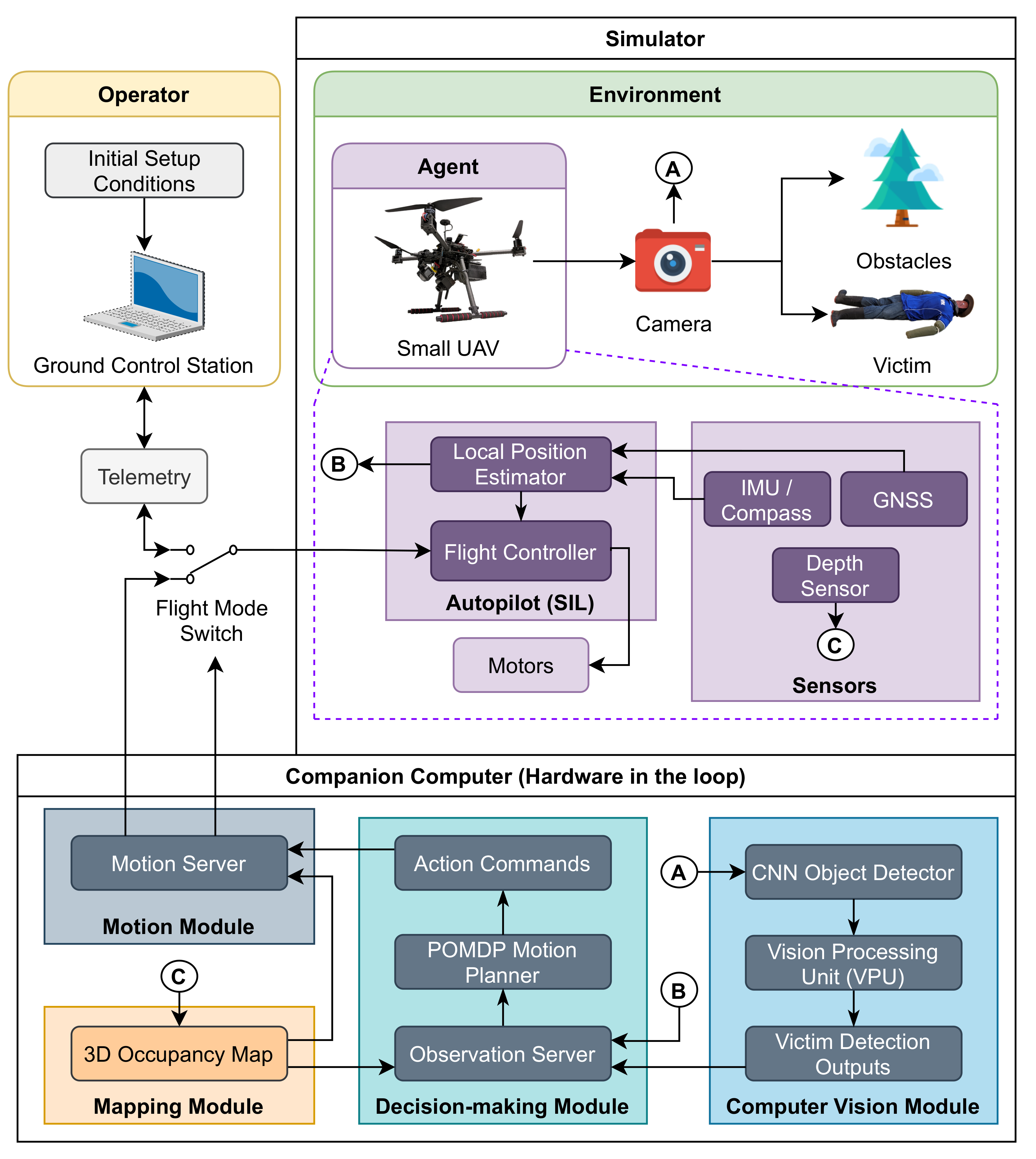
Figure 2.
System architecture for applications with rich global navigation satellite system (GNSS) coverage. The environment, UAV, payloads, victim, and obstacles are emulated in a simulator. The computer vision, decision-making, mapping, and motion modules run in hardware in the loop (HIL) using a companion computer.
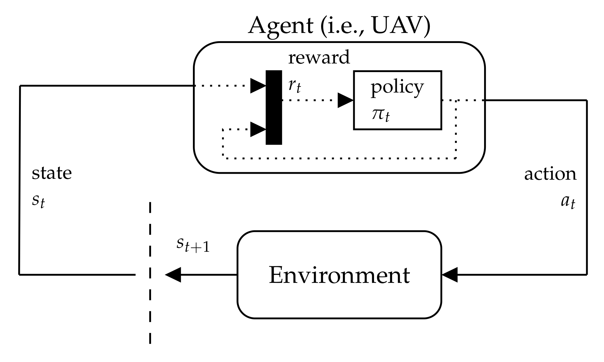
Figure 3.
Interaction between the UAV (or agent) and the environment under the framework of Markov decision processes (MDPs).
Figure 3.
Interaction between the UAV (or agent) and the environment under the framework of Markov decision processes (MDPs).
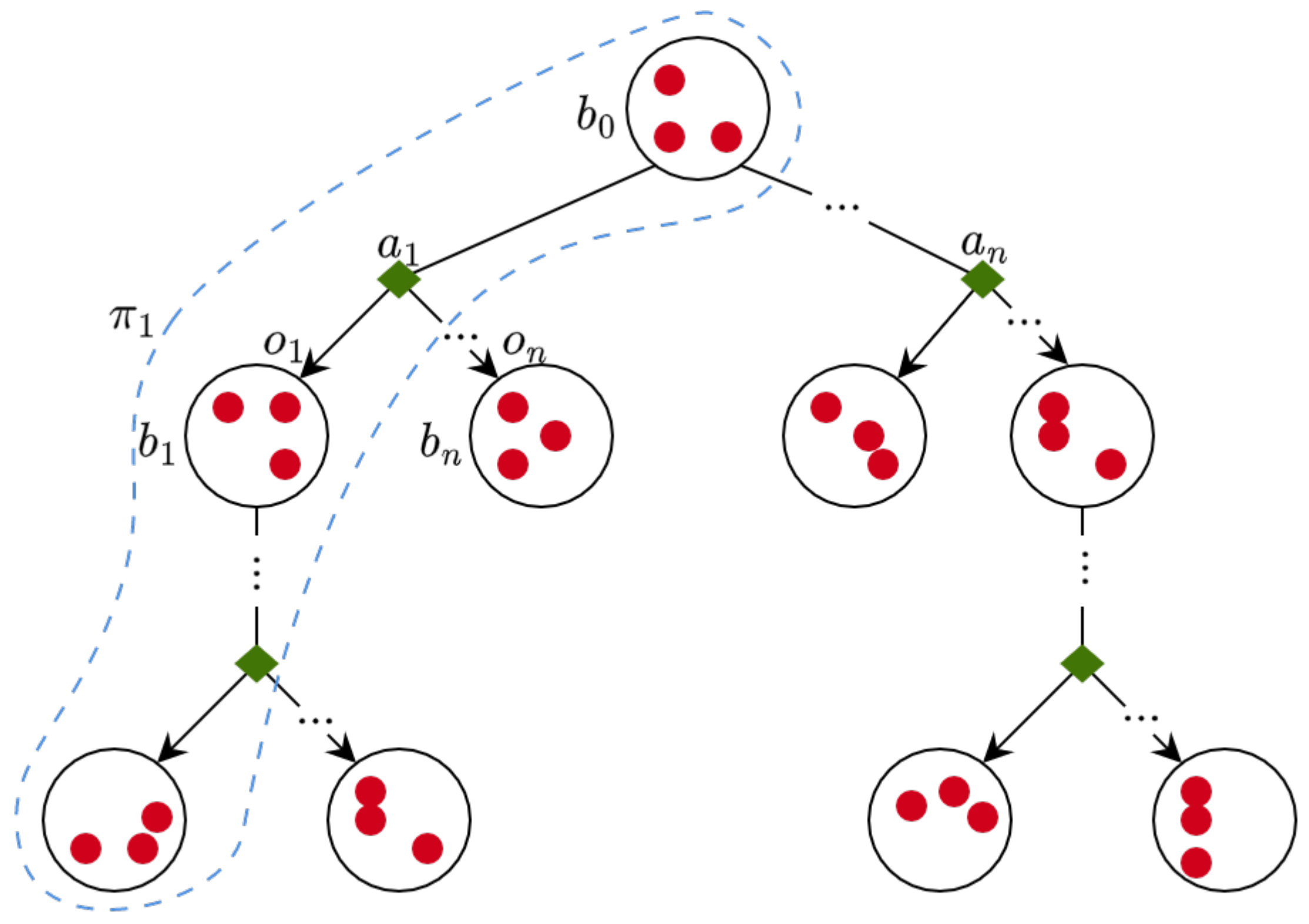
Figure 4.
Belief tree and motion policy representation in partially observable MDPs (POMDPs). Each circle illustrates the system belief as the probability distribution over the system states (red dots). When an observation is made, the belief distribution is subsequently updated.
Figure 4.
Belief tree and motion policy representation in partially observable MDPs (POMDPs). Each circle illustrates the system belief as the probability distribution over the system states (red dots). When an observation is made, the belief distribution is subsequently updated.
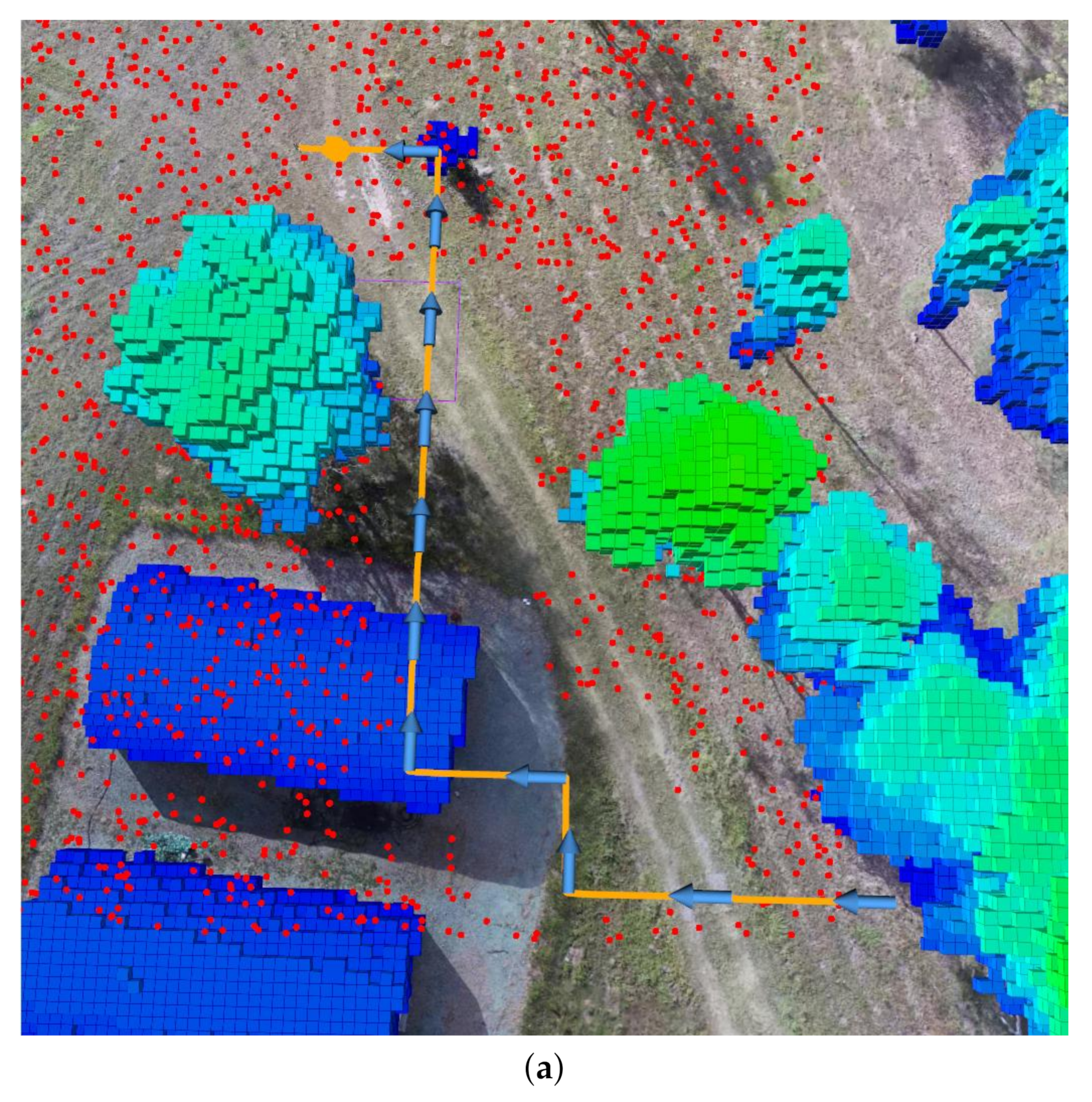
Figure 5.
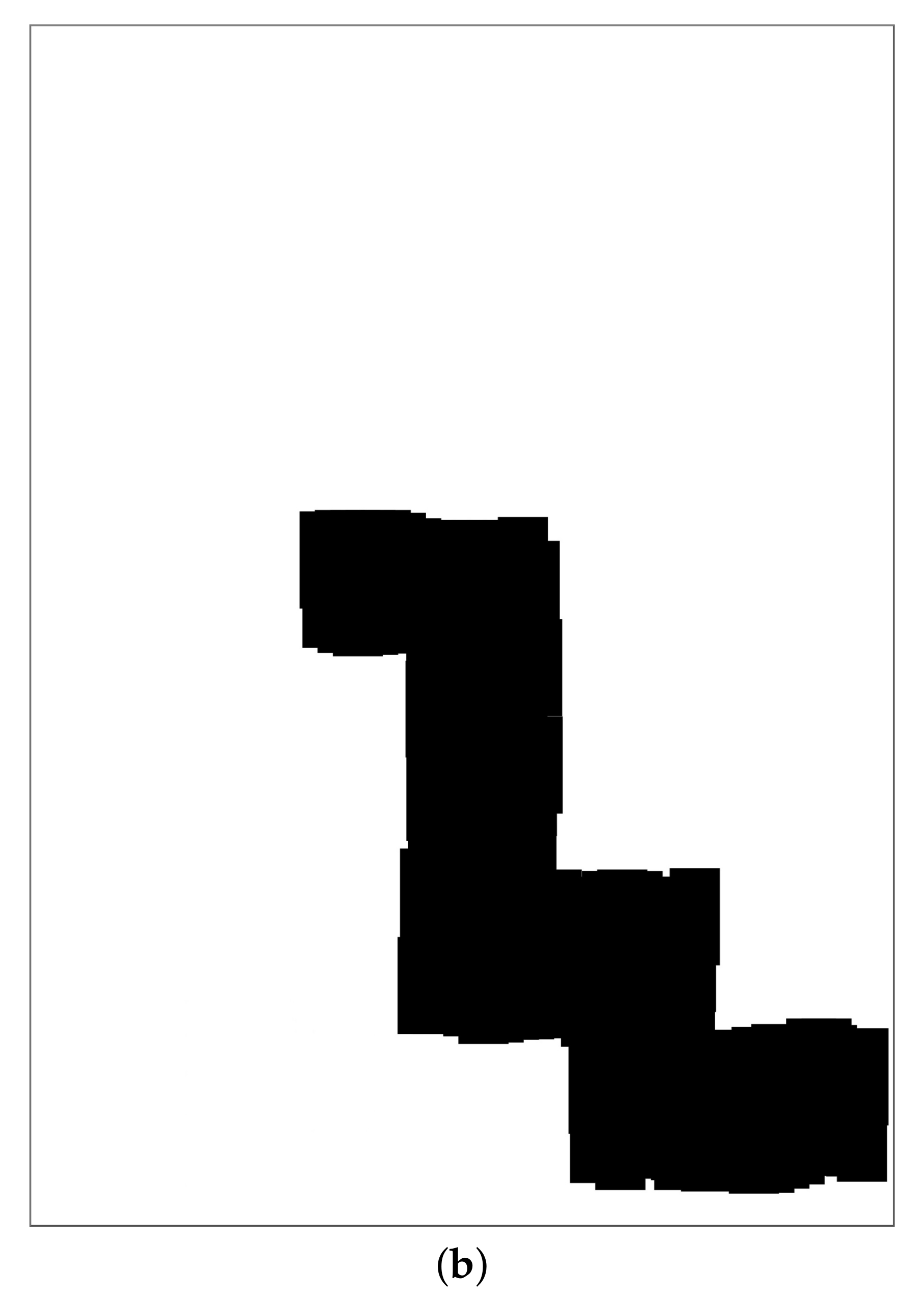
Example of a traversed path by the UAV and its corresponding footprint map. (a) Traversed path of the UAV (orange splines) in a simulated environment. The arrows indicate actions taken by the UAV per time step. Environment obstacles are depicted with blue and green blocks, and the believed victim location points are shown using a red point cloud. (b) Accumulated traced footprint using the extent of the camera’s FOV. Explored areas are depicted in black and unexplored areas in white. The higher the overlap of explored areas after taking an action , the higher the footprint overlap cost.
Figure 5.
Example of a traversed path by the UAV and its corresponding footprint map. (a) Traversed path of the UAV (orange splines) in a simulated environment. The arrows indicate actions taken by the UAV per time step. Environment obstacles are depicted with blue and green blocks, and the believed victim location points are shown using a red point cloud. (b) Accumulated traced footprint using the extent of the camera’s FOV. Explored areas are depicted in black and unexplored areas in white. The higher the overlap of explored areas after taking an action , the higher the footprint overlap cost.
Figure 6.
Field of view (FOV) projection and footprint extent of a vision-based sensor. The camera setup on the UAV frame defines as the pointing angle from the vertical (or pitch) and determines the coordinates of the footprint corners c.
Figure 6.
Field of view (FOV) projection and footprint extent of a vision-based sensor. The camera setup on the UAV frame defines as the pointing angle from the vertical (or pitch) and determines the coordinates of the footprint corners c.
Figure 7.
QUT Samford Ecological Research Facility (SERF) virtual environment setup. (a) Property boundaries of SERF (orange) and simulated region of interest (red). (b) Isometric view of the virtual SERF instance in Gazebo using a high-resolution red, green, blue (RGB) mosaic as the terrain texture. (c) Collected georeferenced LiDAR at SERF using a Hovermap mapper (Emesent Pty Ltd., QLD, Australia). LiDAR data are used to set accurate building and tree canopy heights in the simulated environment.
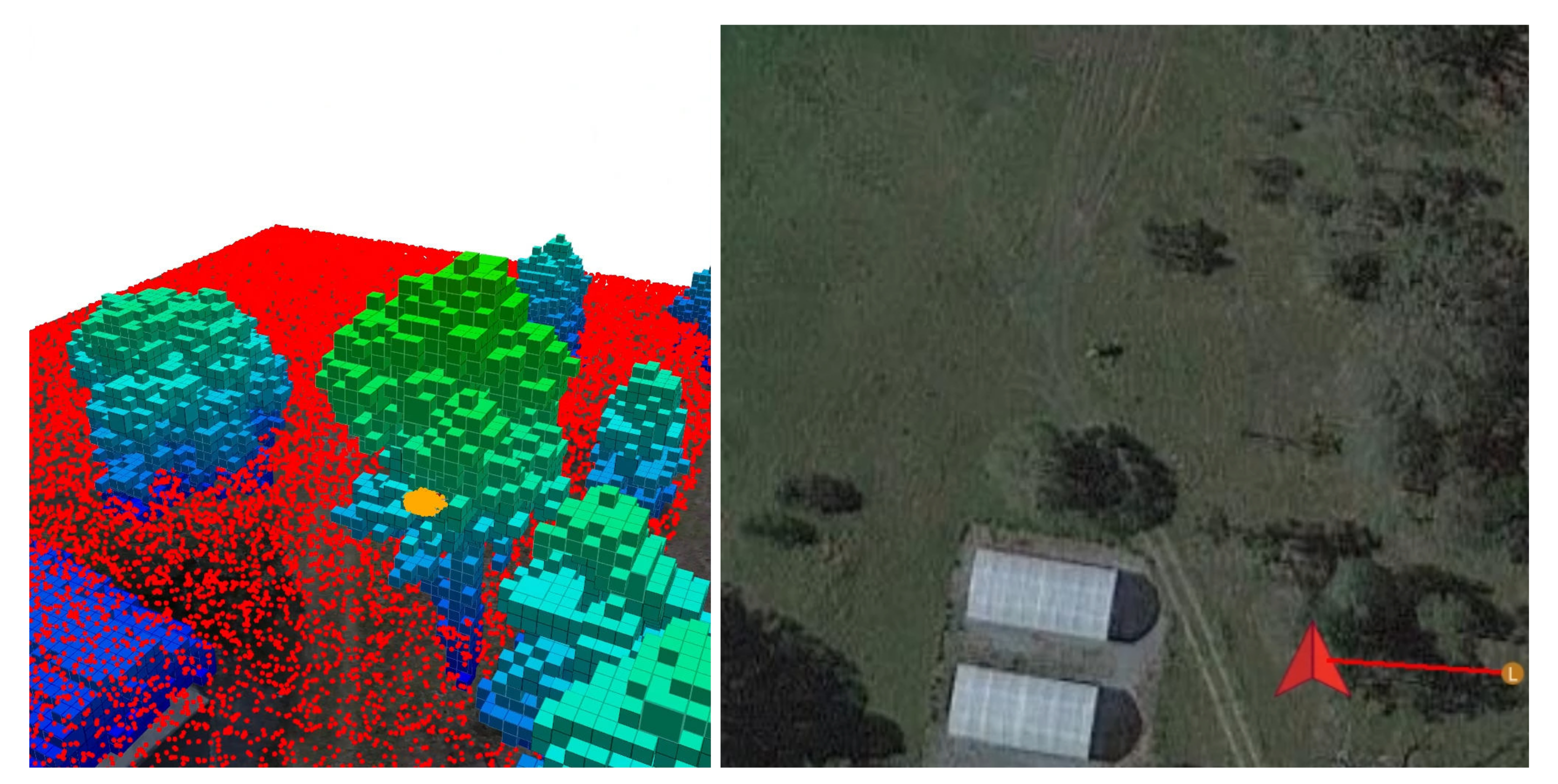
Figure 8.
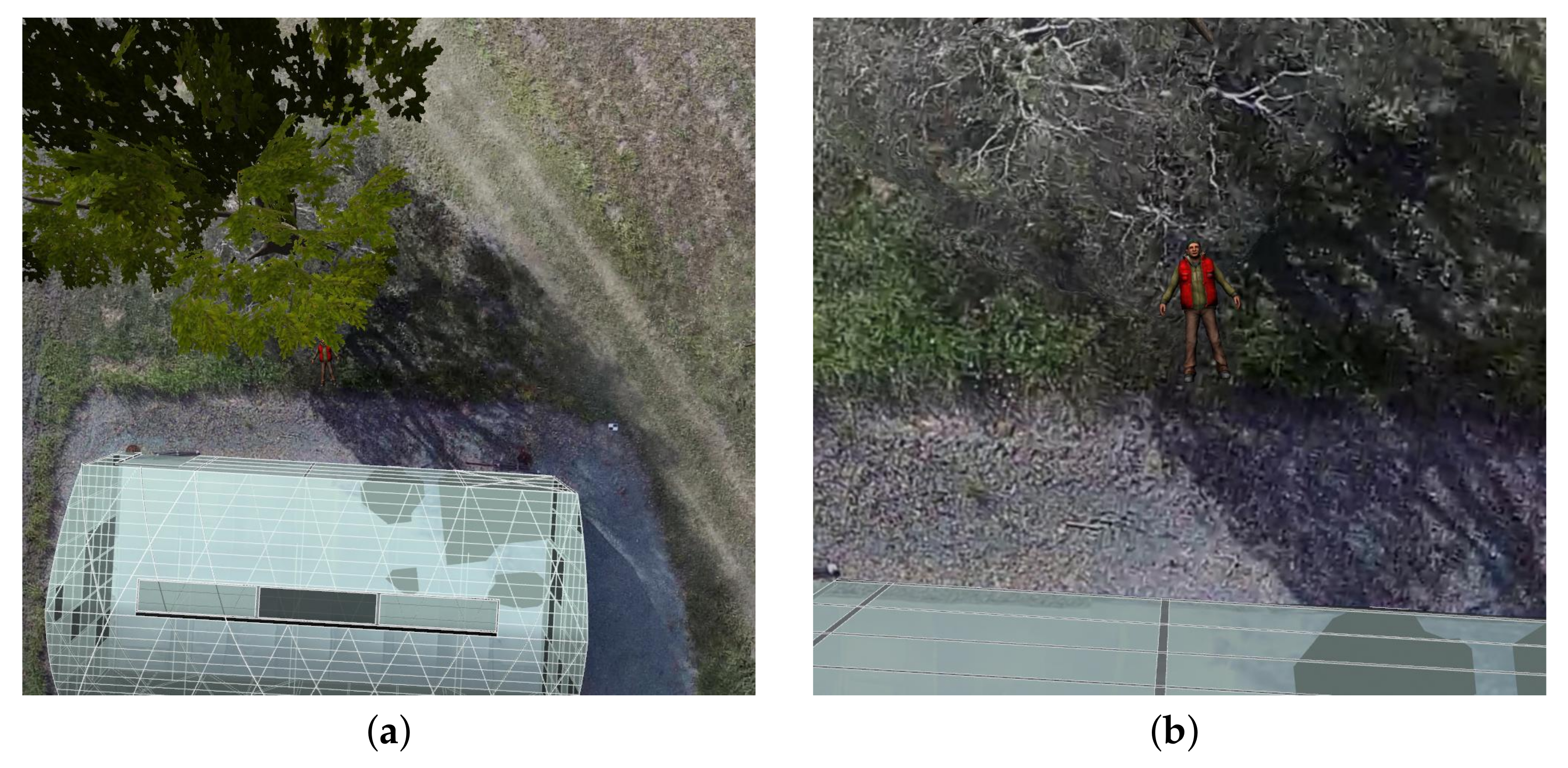
Top-down visualisation and detection challenges of the victim placed at location L2. (
a) Partial occlusion of the victim from the tree branches and leaves. (
b) Magnified view of the victim from
Figure 8a.
Figure 8.
Top-down visualisation and detection challenges of the victim placed at location L2. (
a) Partial occlusion of the victim from the tree branches and leaves. (
b) Magnified view of the victim from
Figure 8a.
Figure 9.
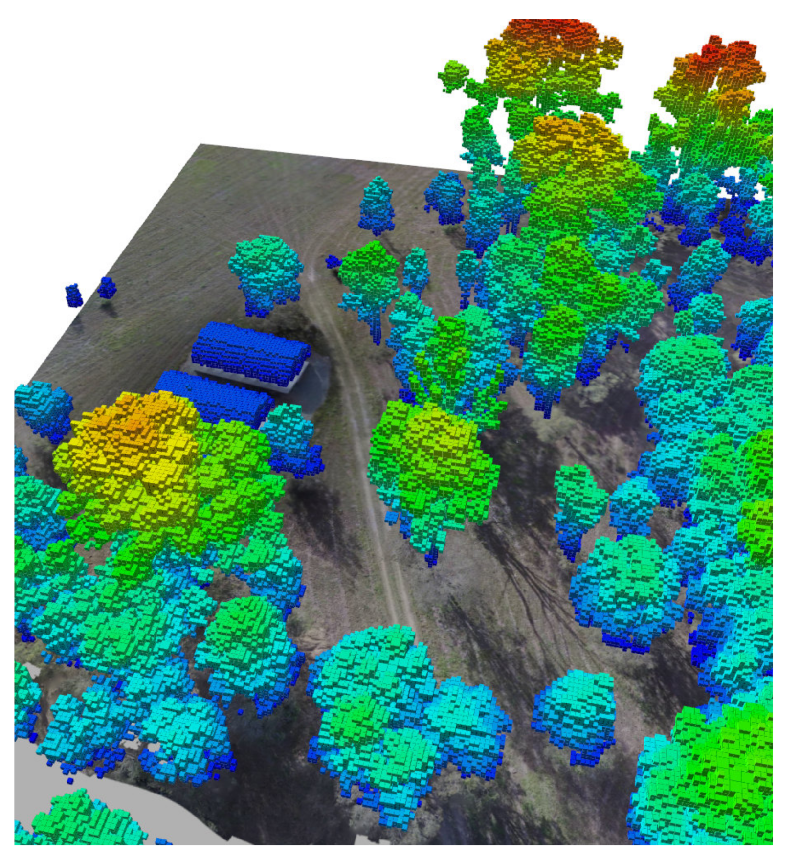
Three-dimensional (3D) occupancy map from the Hovermap LiDAR data of The Samford Ecological Research Facility (SERF). Occupied cells represent the physical location of various tree species and greenhouses present at SERF.
Figure 9.
Three-dimensional (3D) occupancy map from the Hovermap LiDAR data of The Samford Ecological Research Facility (SERF). Occupied cells represent the physical location of various tree species and greenhouses present at SERF.
Figure 10.
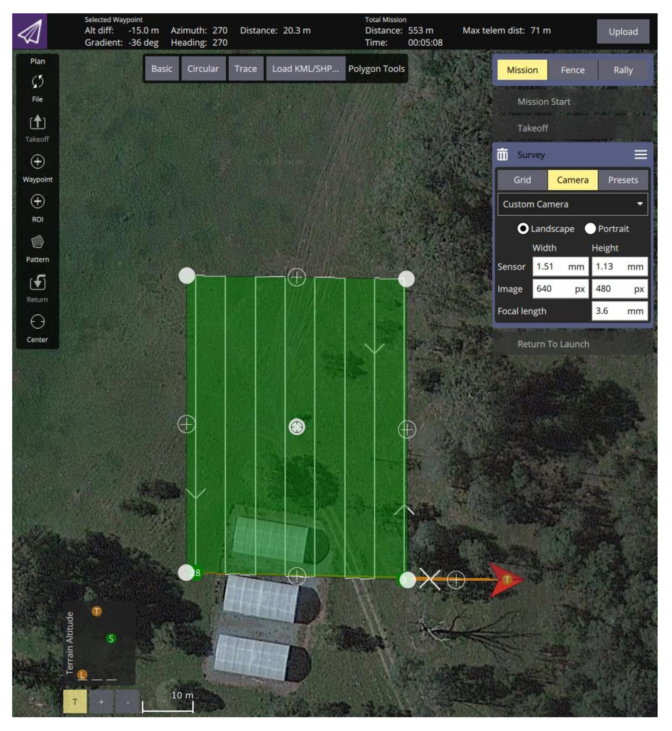
Designed flight plan that the UAV follows in mission mode. The survey is set for a single pass of the setup at a constant height of 20 m, UAV velocity of 2 m/s, and overlap of 30%.
Figure 10.
Designed flight plan that the UAV follows in mission mode. The survey is set for a single pass of the setup at a constant height of 20 m, UAV velocity of 2 m/s, and overlap of 30%.
Figure 11.
Probabilistic distribution of initial UAV and victim position belief across the survey extent. The UAV position belief (orange points) follows a normal distribution with mean equals to and standard deviation of 1.5 m. The victim position belief (red points) follow a uniform distribution, whose limits are equivalent to the survey extent of the flight plan from mission mode.
Figure 12.
Probabilistic distribution of initial UAV and victim position belief under hybrid flight mode. The UAV position belief (orange points) follows a normal distribution, with a mean equals to the current UAV position where a potential victim is first detected, and standard deviation of 1.5 m. The victim position belief (red points) follow a uniform distribution whose limits are equivalent to the extent of the camera’s FOV.
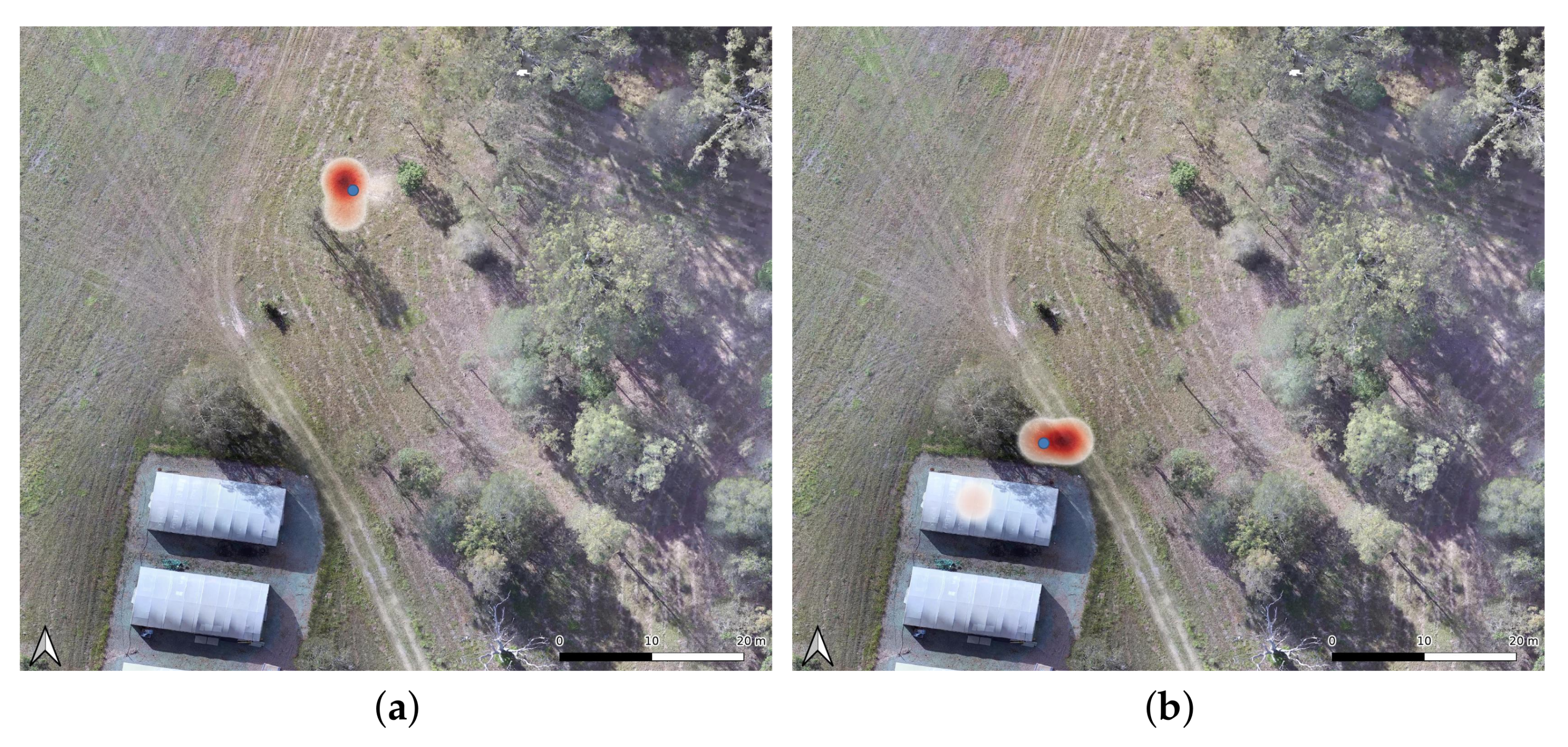
Figure 13.
Heatmaps from recorded GNSS coordinate points from detections in mission mode. The amount of false positive locations were triggered by the CNN model from detecting other objects as people during the survey. (a) First victim location (blue dot) in an open area. (b) Second victim location (blue dot) nearby a tree.
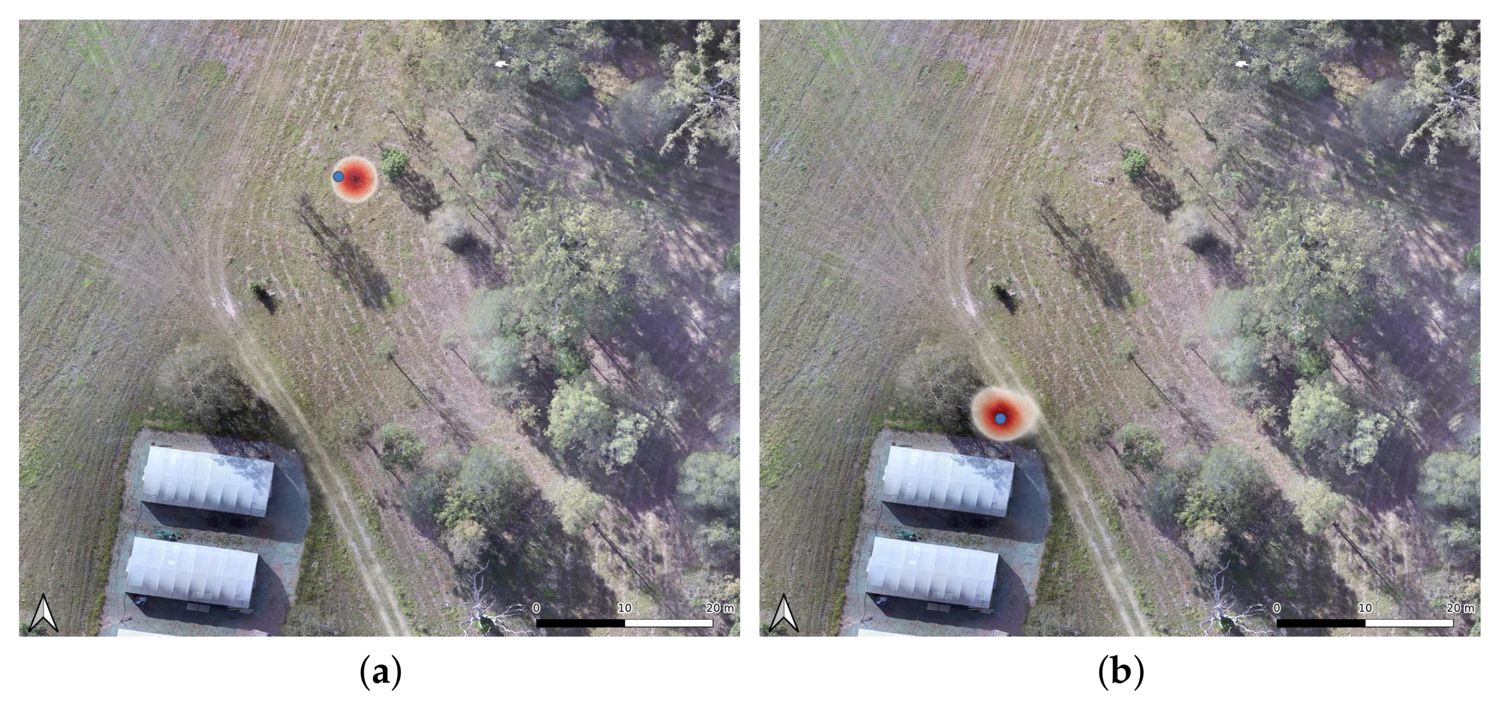
Figure 14.
GNSS coordinates’ heatmaps of confirmed victim detections by the POMDP-based motion planner in offboard flight mode. (a) First victim location (blue dot) in an open area. (b) Second victim location (blue dot) nearby a tree.
Figure 14.
GNSS coordinates’ heatmaps of confirmed victim detections by the POMDP-based motion planner in offboard flight mode. (a) First victim location (blue dot) in an open area. (b) Second victim location (blue dot) nearby a tree.
Figure 15.
GNSS coordinates’ heatmaps of confirmed victim detections by the POMDP-based motion planner in hybrid flight mode. (a) First victim location (blue dot) in an open area. (b) Second victim location (blue dot) nearby a tree.
Figure 15.
GNSS coordinates’ heatmaps of confirmed victim detections by the POMDP-based motion planner in hybrid flight mode. (a) First victim location (blue dot) in an open area. (b) Second victim location (blue dot) nearby a tree.
Figure 16.
Most common object visualisations that triggered false positive readings of people in mission mode. Other objects wrongly detected as people included trees, greenhouse rooftops, and to a lesser degree, bare grass.
Figure 16.
Most common object visualisations that triggered false positive readings of people in mission mode. Other objects wrongly detected as people included trees, greenhouse rooftops, and to a lesser degree, bare grass.
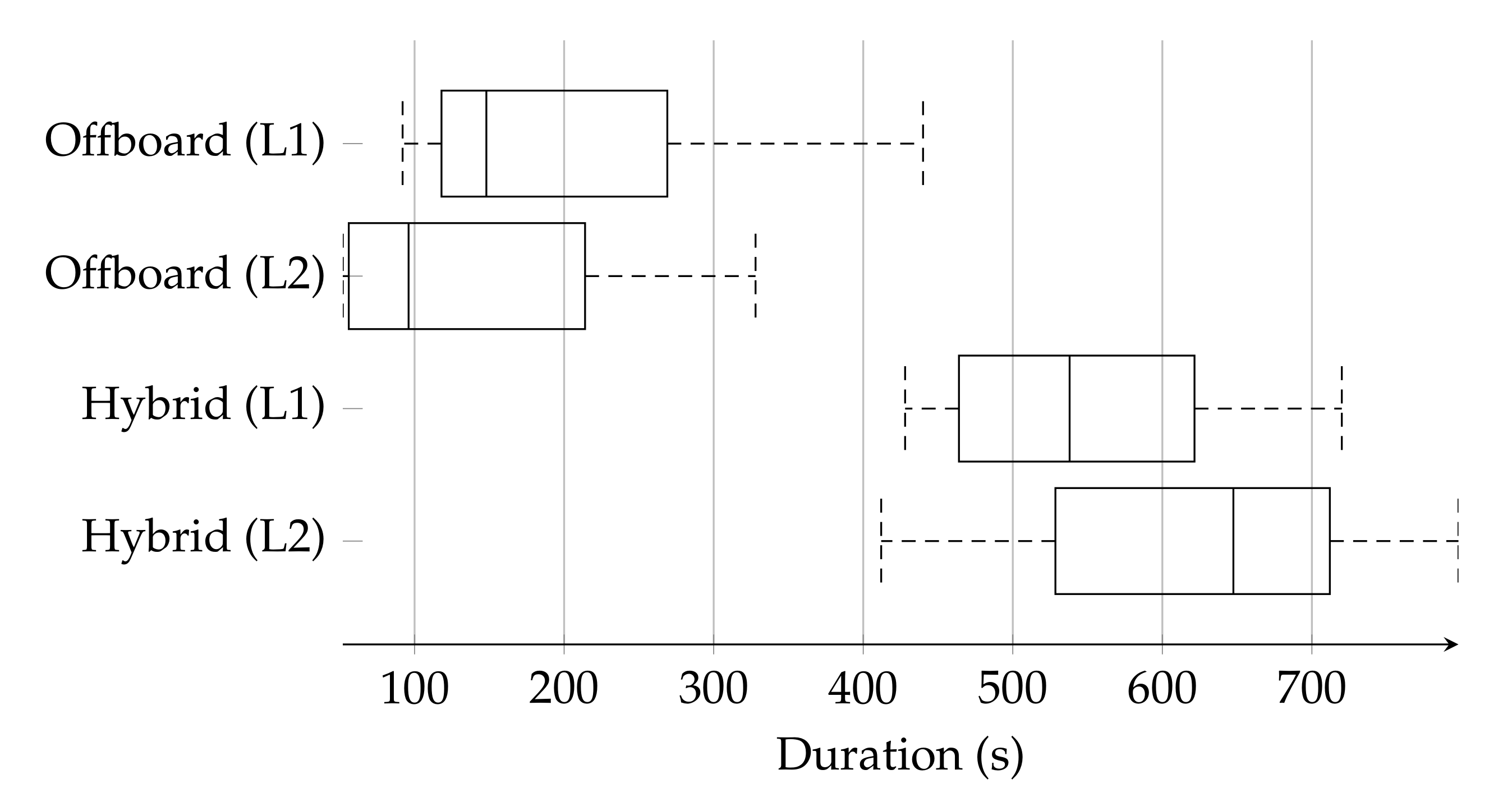
Figure 17.
Distribution frequency of the elapsed time until the POMDP-based motion planner confirmed a detected victim in a trivial (L1) and complex (L2) locations.
Figure 17.
Distribution frequency of the elapsed time until the POMDP-based motion planner confirmed a detected victim in a trivial (L1) and complex (L2) locations.
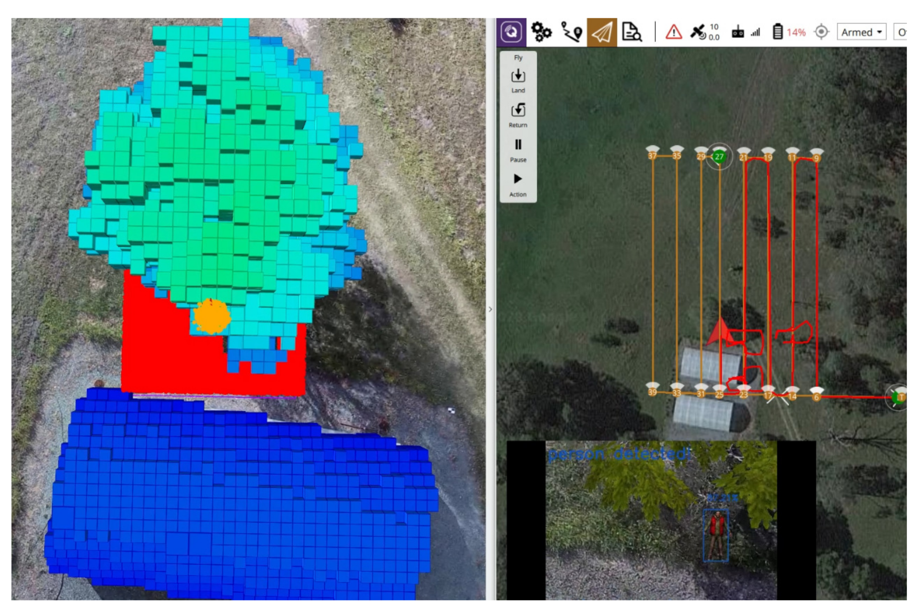
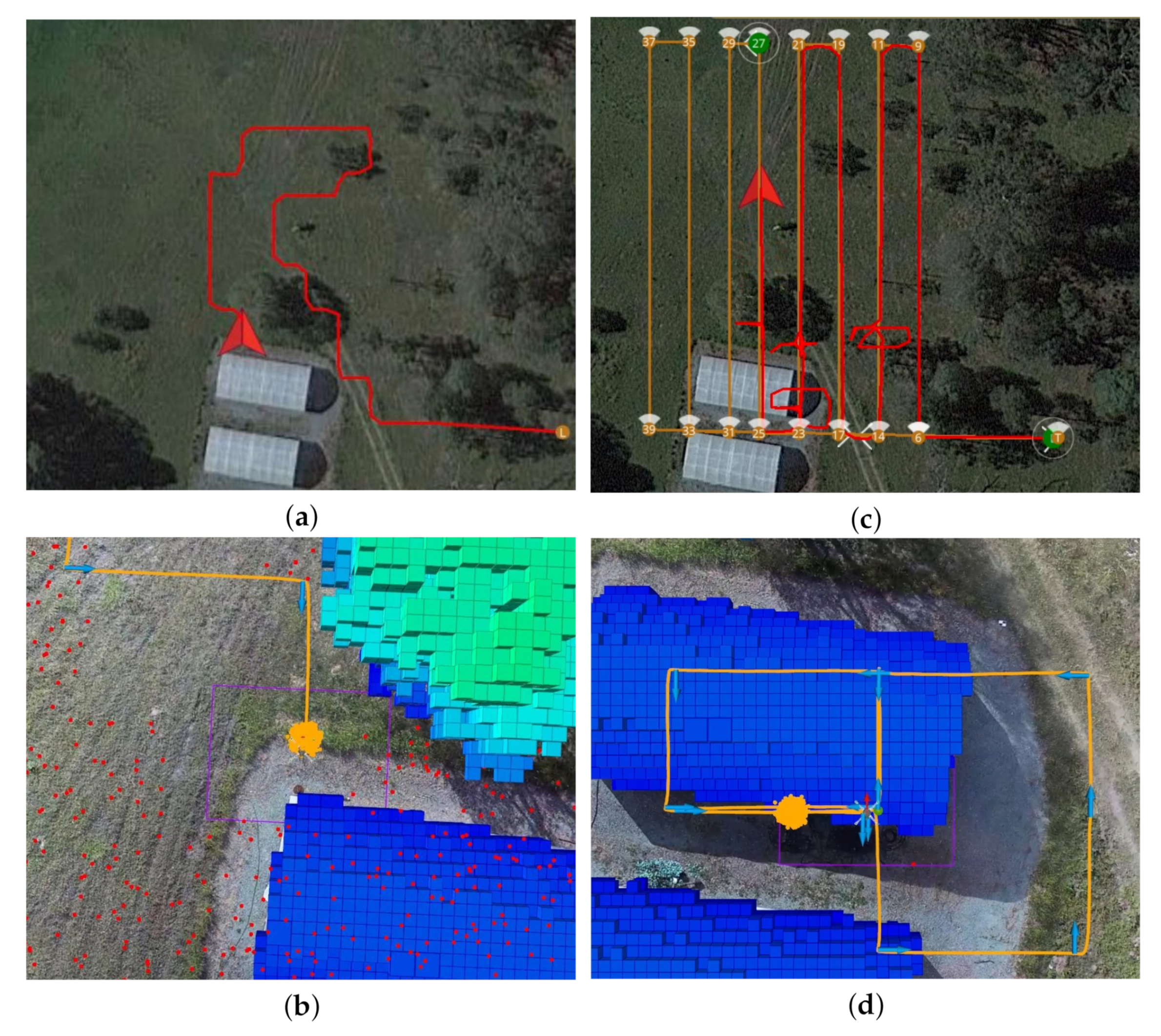
Figure 18.
Illustration of two traversed paths using the proposed POMDP-based motion planner. (a) Traversed path of the UAV in offboard mode. (b) Probabilistic belief locations of the UAV (orange) and victim (red), the latter covering the entire surveyed area. (c) Traversed path of the UAV in hybrid mode. (d) Common path pattern by the UAV to confirm or discard positive detections sent by the computer vision module.
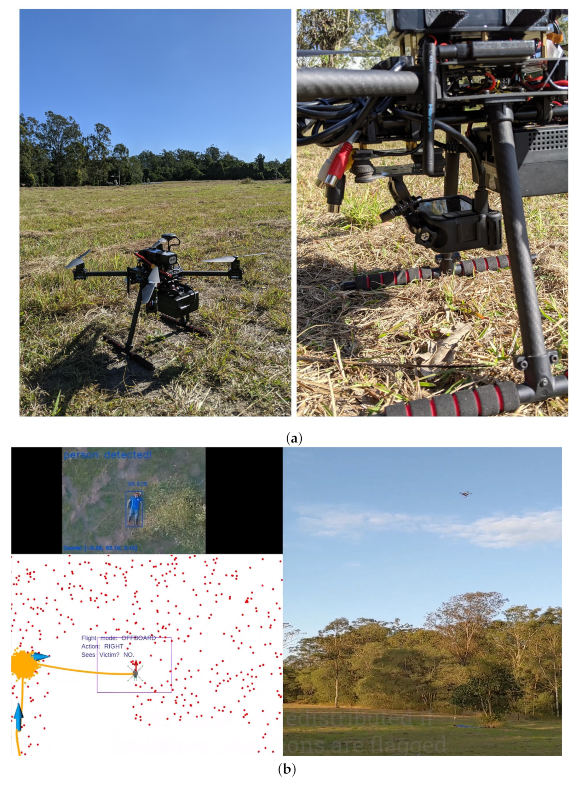
Figure 19.
Demonstration of the presented UAV system in hardware with real flight tests at QUT SERF. (a) Holybro X500 quadrotor UAV frame kit with UP2 as a companion computer and a GoPro Hero 9 as RGB camera. (b) UAV detecting an adult mannequin for the first time while navigating in offboard flight mode.
Table 1.
Set of action commands comprised of local position commands referenced to the world coordinate frame. The system keeps records of its current local position at time step k, and calculates as the change of position magnitude of coordinates , and from time step k to time step .
Table 1.
Set of action commands comprised of local position commands referenced to the world coordinate frame. The system keeps records of its current local position at time step k, and calculates as the change of position magnitude of coordinates , and from time step k to time step .
| | | |
|---|
| Forward | | | |
| Backward | | | |
| Left | | | |
| Right | | | |
| Up | | | |
| Down | | | |
| Hover | | | |
Table 2.
Applied reward values to the reward function R, defined in Algorithm 1.
Table 2.
Applied reward values to the reward function R, defined in Algorithm 1.
| Variable | Value | Description |
|---|
| | Cost of UAV crash |
| | Cost of UAV breaching safety limits |
| | Reward for detecting potential victim |
| | Reward for confirmed victim detection |
| | Cost per action taken |
| | Footprint overlapping cost |
Table 3.
Flight plan parameters for mission mode.
Table 3.
Flight plan parameters for mission mode.
| Property | Value |
|---|
| UAV altitude | 20 m |
| UAV velocity | 2 m/s |
| Camera lens width | 1.51 mm |
| Camera lens height | 1.13 mm |
| Camera focal length | 3.6 mm |
| Image resolution | 640 by 480 px |
| Overlap | 30% |
| Bottom right waypoint | −27.3897972, 152.8732300 |
| Top right waypoint | −27.3892651, 152.8732300 |
| Top left waypoint | −27.3892593, 152.8728180 |
| Bottom left waypoint | −27.3897858, 152.8728180 |
Table 4.
Initial conditions set to the POMDP motion planner.
Table 4.
Initial conditions set to the POMDP motion planner.
| Variable | Description | Value |
|---|
| Maximum UAV altitude | 21 m |
| Minimum UAV altitude | 5.25 m |
| Initial UAV position | (−27.3897972, 152.8732300, 20 m) |
| UAV Heading | 0 |
| UAV climb step | 2 m |
| Frame overlap | 30% |
| Camera pitch angle | 0 |
| Minimum detection confidence | 30% |
| Confidence threshold | 85% |
| Discount factor | 0.95 |
| Time step interval | 4 s |
| Maximum flying time | 8 min |
Table 5.
Accuracy and collision metrics of the system to locate a victim at two locations (L1 and L2). Each setup was evaluated for 20 iterations.
Table 5.
Accuracy and collision metrics of the system to locate a victim at two locations (L1 and L2). Each setup was evaluated for 20 iterations.
| Setup | Detections (%) | Misses (%) | Non-Victims (%) | Collisions (%) |
|---|
| Mission (L1) | | | | |
| Mission (L2) | | | | |
| Offboard (L1) | | | | |
| Offboard (L2) | | | | |
| Hybrid (L1) | | | | |
| Hybrid (L2) | | | | |
Table 6.
Average duration among flight modes to locate the victim. Here, M1, M2, and M3 refer to mission, offboard, and hybrid flight modes, respectively.
Table 6.
Average duration among flight modes to locate the victim. Here, M1, M2, and M3 refer to mission, offboard, and hybrid flight modes, respectively.
| Condition | Duration M1 (s) | Duration M2 (s) | Duration M3 (s) |
|---|
| Victim at Location 1 | 89 | 197 | 238 |
| Victim at Location 2 | 139 | 144 | 353 |
| Entire surveyed area | 256 | — | 622 |


 ,
, 


