Article

Knowledge-Aided Ground Moving Target Relocation for Airborne Dual-Channel Wide-Area Radar by Exploiting the Antenna Pattern Information

1
Beijing Institute of Radio Measurement, Beijing 100854, China
2
School of Information and Communication Engineering, Beijing University of Posts and Telecommunications, Beijing 100876, China
3
National Laboratory of Radar Signal Processing, Xidian University, Xi’an 710071, China
*
Author to whom correspondence should be addressed.
Remote Sens. 2021, 13(22), 4724; https://0-doi-org.brum.beds.ac.uk/10.3390/rs13224724
Submission received: 1 October 2021 / Revised: 12 November 2021 / Accepted: 16 November 2021 / Published: 22 November 2021

Abstract

:
This paper addresses the problem of ground moving target relocation (GMTR) for airborne dual-channel wide-area radar systems. The monopulse technique can be utilized to perform GMTR. However, in real conditions, the GMTR performance degrades greatly due to the effect of channel mismatch. To tackle this problem, prior knowledge of the antenna pattern information is fully utilized to improve the GMTR performance, and a knowledge-aided GMTR algorithm (KA-GMTR) for airborne dual-channel wide-area radar is proposed in this paper. First, the GMTR model for the two receiving channels is analyzed. The channel mismatch model is constructed, and its expression is derived. Then, the channel mismatch phase error is well estimated by exploiting the prior antenna pattern information based on the least squares (LS) method. Meanwhile, the knowledge-aided monopulse curve (KA-MPC) is derived to perform the direction of arrival (DOA) estimation for potential targets. Finally, KA-GMTR, based on the KA-MPC, is performed to estimate the azimuth offsets and relocate the geometry positions of the potential targets when channel mismatch occurs. Moreover, the target relocation performance is analyzed, and the intrinsic reason that degrades the target relocation accuracy is figured out. The performance assessment based on airborne real-data, also in comparison to the conventional GMTR method, has demonstrated that our proposed KA-GMTR algorithm offers preferable target relocation results under channel mismatch scenarios.

1. Introduction

Airborne wide-area radar [1,2,3,4,5,6] has the advantages of large coverage areas and a high revisit ratio, which has been successfully used in military surveillance [1,2,3] and traffic control [4,5,6] in recent years. High resolution imaging and efficient ground moving target indication (GMTI) play an important role in these military and civil applications. For GMTI, two essential problems should be considered. One of the problems is to detect the potential targets in strong clutter environments, and the other is to perform the ground moving target relocation (GMTR).
Clutter suppression is an essential preprocessing step for target relocation, and considerable research work on clutter suppression has been made. Displaced phase center antenna (DPCA) [7] has a long history in the area of clutter cancelation. To overcome the strict constraint among the transmitted pulse repetition frequency (PRF), the airborne platform velocity, and the spacing of phase centers, space time adaptive processing (STAP) has been developed [8]. However, the optimum STAP processor suffers from plenty of limitations in engineering application, such as the requirement of a large number of training samples, the computational complexity burden in the covariance matrix inversion operation, and the severe heterogeneous environments. Then, to solve the aforementioned problems, a lot of reduced dimension or reduced rank STAP algorithms such as the joint domain localized (JDL) [9,10,11], the EFA [12], the ΣΔ-STAP [13], the generalized sidelobe canceller (GSC) [14], and other suboptimum methods [15,16,17] have been proposed. In order to solve the problem of insufficient training sample data, the property of covariance matrix is fully exploited to improve the STAP performance in real conditions [18,19,20,21,22]. Moreover, prior knowledge can be incorporated into radar to perform the space-time adaptive beam former, and the KA-STAP has been developed [23,24,25]. In this paper, we focus on the second problem of GMTI to improve the target’s relocation performance.
After clutter suppression, the problem of target relocation is essential. Therefore, the accuracy of GMTR is one of the research hotspots in the study of airborne radar. A moving target usually has an azimuth position shift in the imaging map (SAR image or DBS image) due to the radial velocity (i.e., cross-track motion) [26], and the cross-track motion always introduces the range cell migration (RCM). Keystone transform (KT) [27,28] and second-order keystone transform (SOKT) [29,30] based methods can be exploited to perform the range cell migration correction (RCMC). After RCMC, the radial velocity can be estimated with radon transform, which is useful to relocate the potential targets [31]. For the multichannel synthetic-aperture radar (SAR) system, along-track interferometry (ATI) can be used [32,33,34,35,36,37] to relocate the potential targets. Along-track motion of a moving target will have an additional phase term, and the additional phase term can be approximated by time-frequency analysis methods [38], such as Wigner–Ville distribution [39] or FrFT [40]. In addition, the Doppler parameters estimation methods, such as the azimuth compression function [41,42] or the quadratic-term ATI phase estimation method [43,44], are also useful tools to estimate the along-track velocity and relocate the potential targets. Multiple-output (MIMO) radar techniques are discussed to achieve simultaneous adaptive clutter cancellation and target relocation [45,46]. In the aforementioned GMTR methods, the scene of target relocation is mainly considered in the spaceborne/airborne single-channel or multi-channel SAR radar system. The single-channel system performs not well in real conditions [28,29,38,39,40], and more antennas always mean higher hardware cost in multi-channel systems [36,43,44,45,46]. Moreover, most of the airborne radar systems are dual-channel due to weight and volume constraints. Since few works are focused on GMTR for the airborne dual-channel wide-area radar system, it is quite essential to study the dual-channel system further. Besides, many scholars have investigated the problem of GMTR under ideal conditions [37,38,39]. In practical applications, especially for the airborne dual-channel wide-area radar, channel mismatch is inevitable due to the impact of electron devices, which degrades the performance of target relocation. In addition, the adjacent receiving channels may differ in amplitude and phase even for the same radar system. These errors will further decrease the targets relocation accuracy and degenerate the direction of arrival (DOA) estimation result. In worse cases, channel mismatch may blur the tracks of the potential targets and increase the false alarms.
The target relocation problem in airborne wide-area radar is first analyzed in [6], and the flowchart to process the GMTI data for each antenna look direction and each scan is introduced in detail. In this airborne wide-area radar, iterative 2D-calibration [47], which brings in a large computational cost in the real radar system, is used for preprocessing the channel imbalances. A channel balancing algorithm based on subsections selection is proposed in [48], and the accuracy of channel interference phase largely depends on the selected subsections. This method may suffer from performance degradation when the selected subsections are not appropriate. To solve this problem, a knowledge-based indirect target relocation method that performs indirect target relocation based on the neighboring clutter information and not the channel mismatch correction is proposed in [49]. This indirect target relocation method performs well in the scene where the detected target is far away from the main lobe of the clutter area. Meanwhile, a knowledge-based direct target relocation method, which works well under the assumption that the boresight angle is accurately compensated, is discussed in [50]. However, the channel mismatch is always inevitable. Some of the slowly moving targets may locate the main lobe of the clutter area in real conditions, and the boresight angle cannot be fully compensated. All the mentioned factors will degenerate the target relocation performance greatly.
Considering the fact that plenty of airborne dual-channel wide-area radars are still in service, we focus on performing GMTR based on the monopulse technique. The monopulse technique [51,52,53,54,55,56], which can be used to estimate the DOA of potential targets after STAP processing [57,58], is an essential technique for radar angle estimation. In this paper, an efficient knowledge-aided GMTR (KA-GMTR) for airborne dual-channel wide-area radar is proposed. Precisely, the channel mismatch model for the two receiving channels is constructed and its expression for the channel mismatch phase error is derived. Then, the channel mismatch phase error is well estimated using the prior antenna pattern information, and the DOA estimation for potential targets is performed with this derived KA-MPC. Based on the DOA estimation results, the proposed KA-GMTR method can relocate the azimuth position of the potential targets in the case of channel mismatch. In addition, the target relocation performance is analyzed, and the intrinsic reason that degrades the target relocation accuracy is figured out. Finally, airborne real-data experimental results demonstrate that the proposed KA-GMTR method can effectively concentrate the tracks of the potential targets and decrease the false alarm in the channel mismatch scenarios.
The remainder of this paper is organized as follows. The airborne dual-channel wide-area target relocation model is introduced in Section 2. In Section 3, the channel mismatch model is constructed, and its expression is derived. Then, a novel KA-GMTR framework is proposed in detail. In addition, the target relocation performance is analyzed. Section 4 presents real data results, while the conclusions of this paper are presented in Section 5.

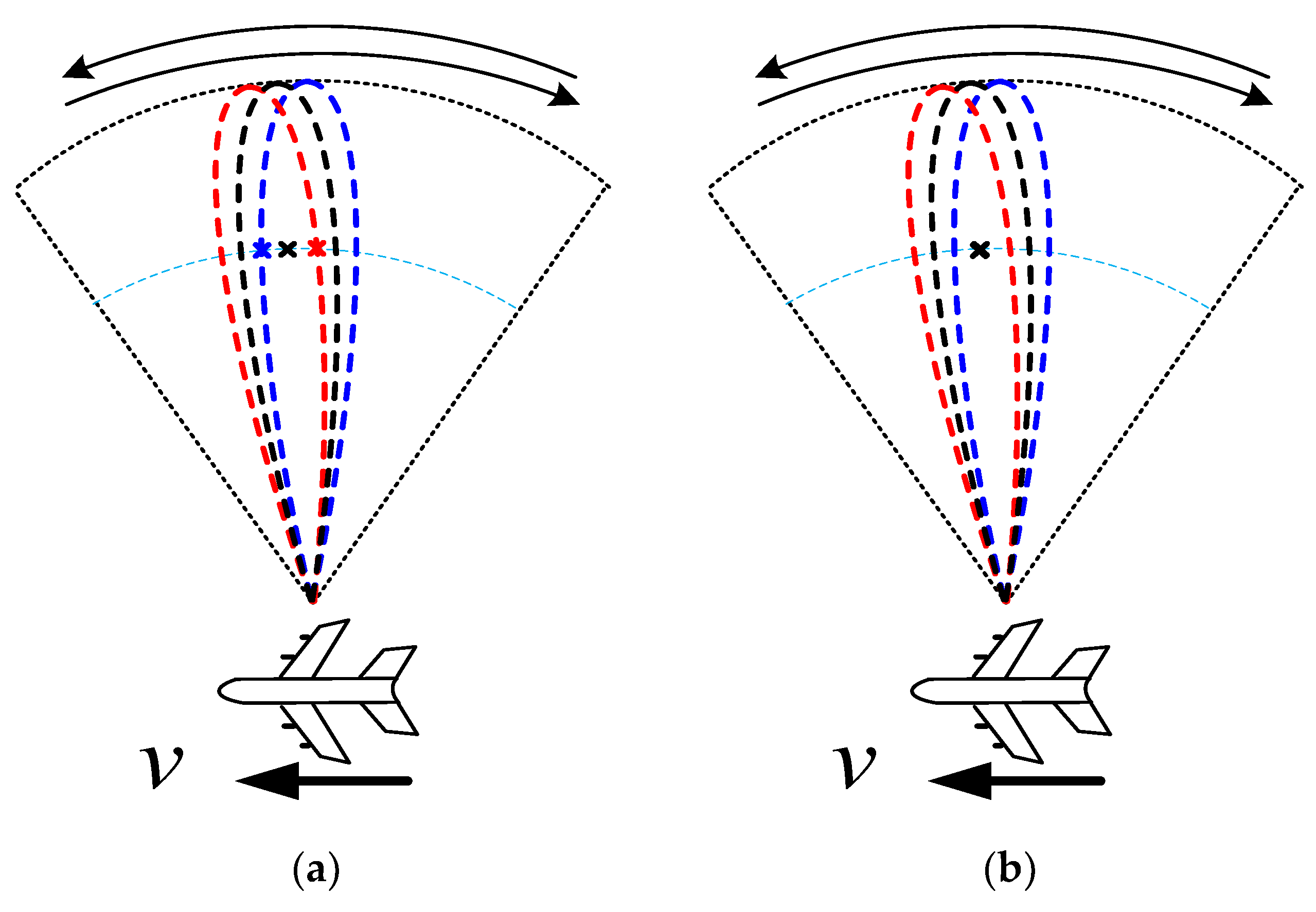
2. Target Relocation Model

Consider an airborne wide-area radar system with a uniform planar array consisting of two channels, as depicted in Figure 1. The airborne platform flies along the Y direction with a constant velocity v at altitude H . θ and η are the squint angle and the elevation angle, respectively. Assuming that C is the equivalent phase center (EPC) [41,42,43,44] of the transmitting channel in the airborne wide-area radar system, A and B are the EPCs of the two receiving channels, respectively. D denotes the distance between A and B . The scene center illustrated by antenna beam is represented by O , and P is a scattering center near O . The instantaneous range from C to the scene center O is denoted by R 0 , and the instantaneous range from C to point P is R 1 . R 2 is the instantaneous range between A and P , and R 3 represents the instantaneous range between B and P . In order to acquire high range resolution, it is supposed that a linear frequency modulated (LFM) signal is used, which can be given by [1,2]
e ( τ ) = rect ( τ T p ) exp [ j 2 π ( f c τ + γ 2 τ 2 ) ]
where γ denotes the LFM rate, τ is the radar fast-time, and Tp represents the transmitted pulse width. By the matched-filtering and range migration correction (RMC) in the range direction [1,2], the received signal can be given by
s 1 ( τ , t ) = w a ( t t c ) sin c [ B ( τ 2 R 1 c ) ] exp ( j 2 π R 1 + R 2 λ )
s 2 ( τ , t ) = w a ( t t c ) sin c [ B ( τ 2 R 1 c ) ] exp ( j 2 π R 1 + R 3 λ )
where w a ( t ) = sin c 2 ( R b tan ( θ ) v ) represents the antenna window function, and R b is the nearest slant range. t c = R tan ( θ c ) v is the beam center crossing time. s i ( τ , t ) is the matched-filtering and range migration correction (RMC) signal for the ith receiving channel, T r represents the pulse repetition interval, and T s = N × T r denotes the coherent processing interval (CPI). N is the pulse number of one CPI. The function sin c ( × ) is defined by sin c ( x ) = sin ( π x ) x .
Under ideal conditions, two receiving channels can be used to construct the sum signal s Σ and the difference signal s Δ , which can be given by
s Σ = s 1 ( τ , t ) + s 2 ( τ , t ) = w a ( t t c ) sin c [ B ( τ 2 R 1 c ) ] [ exp ( j 2 π R 1 + R 2 λ ) + exp ( j 2 π R 1 + R 3 λ ) ]
s Δ = s 1 ( τ , t ) s 2 ( τ , t ) = w a ( t t c ) sin c [ B ( τ 2 R 1 c ) ] [ exp ( j 2 π R 1 + R 2 λ ) exp ( j 2 π R 1 + R 3 λ ) ]
After compensated by the mean slant range (i.e., exp ( j 4 π R 0 λ ) ), (4) and (5) can be rewritten as
s Σ = w a ( t t c ) sin c [ B ( τ 2 R 1 c ) ] exp ( j 4 π R 0 λ ) [ exp ( j 2 π R 1 + R 2 λ ) + exp ( j 2 π R 1 + R 3 λ ) ]
s Δ = w a ( t t c ) sin c [ B ( τ 2 R 1 c ) ] exp ( j 4 π R 0 λ ) [ exp ( j 2 π R 1 + R 2 λ ) exp ( j 2 π R 1 + R 3 λ ) ]
After some algebraic operations (which have been analyzed in Appendix A), (6) and (7) can be simplified as
s Σ = 2 cos ( π R 2 R 3 λ ) w a ( t t c ) sin c [ B ( τ 2 R 1 c ) ] exp ( j π 2 R 1 + R 2 + R 3 4 R 0 λ )
s Δ = 2 j sin ( π R 2 R 3 λ ) w a ( t t c ) sin c [ B ( τ 2 R 1 c ) ] exp ( j π 2 R 1 + R 2 + R 3 4 R 0 λ )
Assuming that a potential target is placed at θ = θ c + δ θ , where δ θ is the azimuth offset, and θ c represents the boresight of the antenna beam, we can then obtain the following expression
sin θ = sin ( θ c + δ θ ) sin θ c + cos θ c δ θ
In Equation (10), first-order Taylor series expansion is used.
As illustrated in Figure 1, we can obtain the following geometry relationship
R 2 R 3 = D sin θ
Substituting (10) and (11) into (8) and (9), which have been analyzed in Appendix B, the final sum channel signal and the difference channel signal can be denoted as
s Σ = 2 cos [ π D ( sin θ c + cos θ c δ θ ) λ ] w a ( t t c ) × sin c [ B ( τ 2 R 1 c ) ] exp ( j π 2 R 1 + R 2 + R 3 4 R 0 λ )
s Δ = 2 j sin [ π D ( sin θ c + cos θ c δ θ ) λ ] w a ( t t c ) × sin c [ B ( τ 2 R 1 c ) ] exp ( j π 2 R 1 + R 2 + R 3 4 R 0 λ )
Then, the monopulse result can be given by [51,52]
K = s Δ s Σ = j tan [ π D ( sin θ c + cos θ c δ θ ) λ ]
After simplification, we have the azimuth offset of the potential target with respect to the antenna boresight, i.e.,
δ θ = λ π D cos θ c arctan ( K im ) tan θ c
where K im is the imaginary part of K . A monopulse curve (MPC) can be drawn by estimating all the azimuth offsets with the antenna geometry configuration under different K im [51], as illustrated in Figure 2. Figure 2 gives the ideal results for the airborne dual-channel radar system. In this simulation, the radar consists of an array of 35 elements spaced 4 mm apart. The 3 dB beamwidth is about 3.1 . In ideal cases, the sum channel signal and the difference channel signal are always perpendicular. From Figure 2c, we can see that different azimuth offsets correspond to different monopulse ratios. We can compute all the azimuth offsets theoretically based on the MPC and relocate the potential targets. However, the above analysis is under the assumption that there is no channel mismatch. The channel mismatch is inevitable in practice. This channel mismatch may distort the estimated azimuth offsets and reduce the GMTR performance. As a result, poor GMTR performance is always inevitable in real conditions. In the following, the uncertain features between the two receiving channels caused by channel mismatch will be effectively modeled and removed.

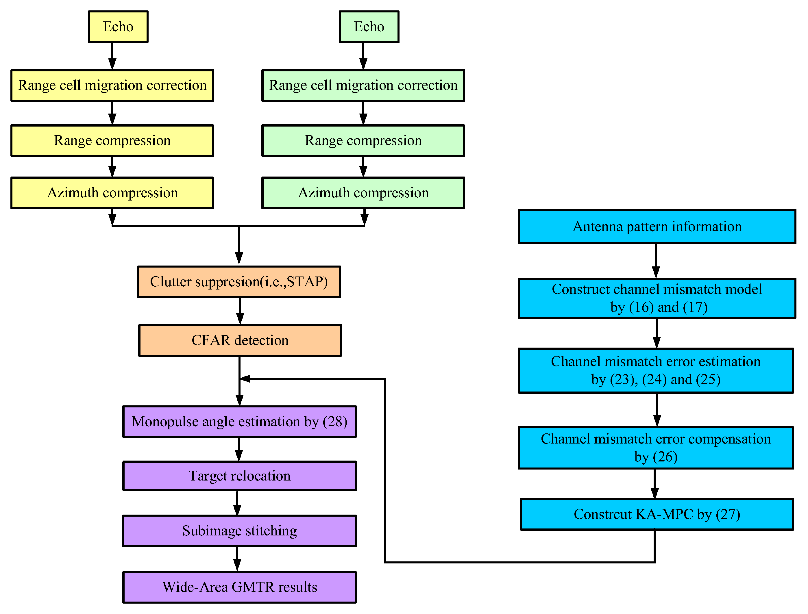
3. Knowledge-Aided Target Relocation by Exploiting the Antenna Pattern Information

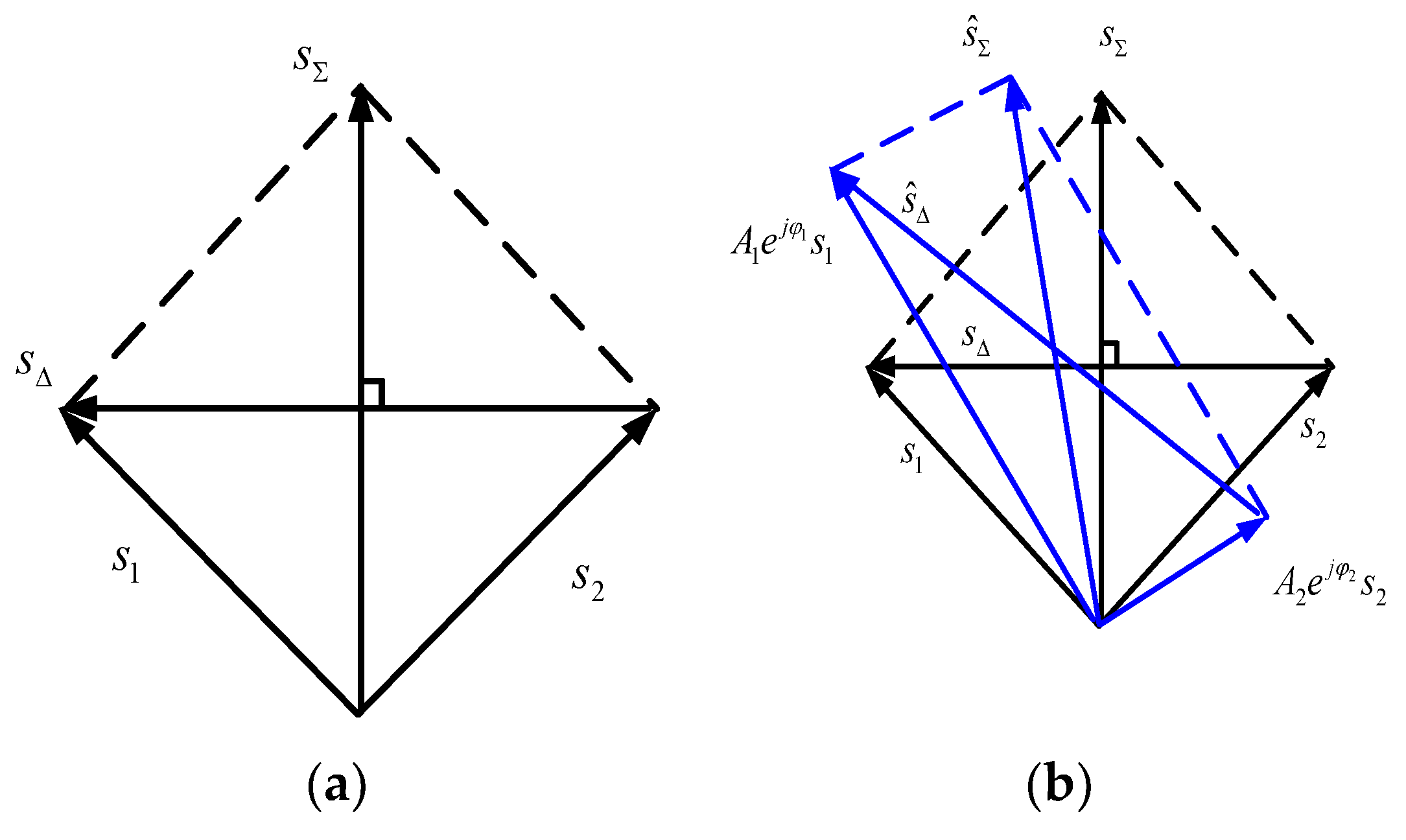
3.1. Channel Mismatch Model

As mentioned in Section 2, the target relocation performance depends largely on the MPC. If the MPC is not correct, the estimated azimuth offsets may be distorted. However, the sum channel signal and the difference channel signal are not perpendicular due to the existence of the channel mismatch, as shown in Figure 3. In practice, the MPC result will distort compared with the ideal conditions. To solve this problem, amplitude error and phase error are introduced to model the channel mismatch, and the expression for the channel mismatch scene can be modeled as follows
s ^ 1 ( τ , t ) = A 1 e j φ 1 w a ( t t c ) sin c [ B ( τ 2 R 1 c ) ] exp ( j 2 π R 1 + R 2 λ )
s ^ 2 ( τ , t ) = A 2 e j φ 2 w a ( t t c ) sin c [ B ( τ 2 R 1 c ) ] exp ( j 2 π R 1 + R 3 λ )
where A i and φ i denote the amplitude error and the phase error for the ith channel, respectively. In practice, the new sum channel signal and the difference channel signal (namely s ^ Σ and s ^ Δ ) in the situation of channel mismatch can be expressed as
s ^ Σ = s ^ 1 ( τ , t ) + s ^ 2 ( τ , t ) = w a ( t t c ) sin c [ B ( τ 2 R 1 c ) ] × [ A 1 e j φ 1 exp ( j 2 π R 1 + R 2 λ ) + A 2 e j φ 2 exp ( j 2 π R 1 + R 3 λ ) ]
s ^ Δ = s ^ 1 ( τ , t ) s ^ 2 ( τ , t ) = w a ( t t c ) sin c [ B ( τ 2 R 1 c ) ] × [ A 1 e j φ 1 exp ( j 2 π R 1 + R 2 λ ) A 2 e j φ 2 exp ( j 2 π R 1 + R 3 λ ) ]
Performing motion compensation by the mean slant range, we can obtain the MPC with some simplification as
K = S ^ Δ S ^ Σ = 1 A 2 A 1 e j ( φ 2 φ 1 + 2 π D s i n θ λ ) 1 + A 2 A 1 e j ( φ 2 φ 1 + 2 π D s i n θ λ )
By using the Euler Formula, which have been analyzed in Appendix C, (20) can be transformed as follows
K = ( 1 A 2 / A 1 × cos ( φ ) ) 2 + ( A 2 / A 1 × sin ( φ ) ) 2 ( 1 + A 2 / A 1 × cos ( φ ) ) 2 + ( A 2 / A 1 × sin ( φ ) ) 2 e j φ ^
where φ = φ 2 φ 1 + 2 π D s i n θ λ , φ ^ = atan ( A 2 / A 1 sin ( φ ) 1 A 2 / A 1 cos ( φ ) ) atan ( A 2 / A 1 sin ( φ ) 1 + A 2 / A 1 cos ( φ ) ) .
In ideal conditions, the equations A 2 = A 1 and φ 2 = φ 1 hold, then we can obtain that
φ ^ i d e a l = atan ( sin ( 2 π λ D sin θ ) 1 cos ( 2 π λ D sin θ ) ) atan ( sin ( 2 π λ D sin θ ) 1 + cos ( 2 π λ D sin θ ) ) = π 2
It can be seen that the ideal condition is just a special case of channel mismatch. However, in practice, A 2 A 1 and φ 2 φ 1 , and we can conclude that the real part of the MPC is not equal to zero (i.e., φ ^ π 2 + 2 k π , k Z ), which means that not all the energy is concentrated on the imaginary part of the MPC. This is the reason that the leaked energy of the real part in the MPC degrades the GMTR performance. In extreme cases (i.e., φ ^ = k π , k Z ), it is hard to estimate the azimuth offsets for the potential targets because the energy in the imaginary part of the MPC is zero. In this case, the imaginary part of the MPC is a horizontal line, and the potential targets cannot be relocated.
Figure 4 gives the comparisons of MPC under different channel mismatch phase errors. The channel mismatch phase errors are changed from −180 degrees to 180 degrees to simulate different channel mismatch scenarios (see the second column). From Figure 4, it is obvious that the imaginary part of the MPC strongly depends on the value of channel mismatch phase error. The imaginary part of the MPC has the minimum values when the channel mismatch phase errors are −180, 0, and 180 degrees. In order to relocate the potential targets, we should estimate the channel mismatch phase error to make the imaginary part of the MPC as high as possible.

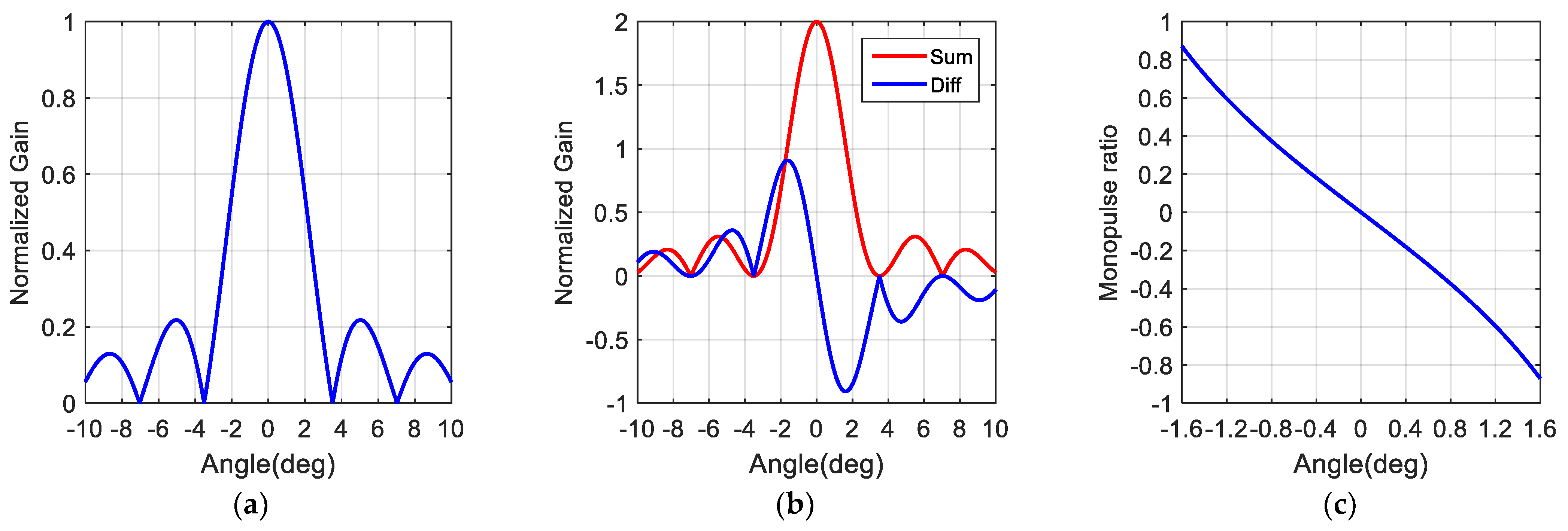
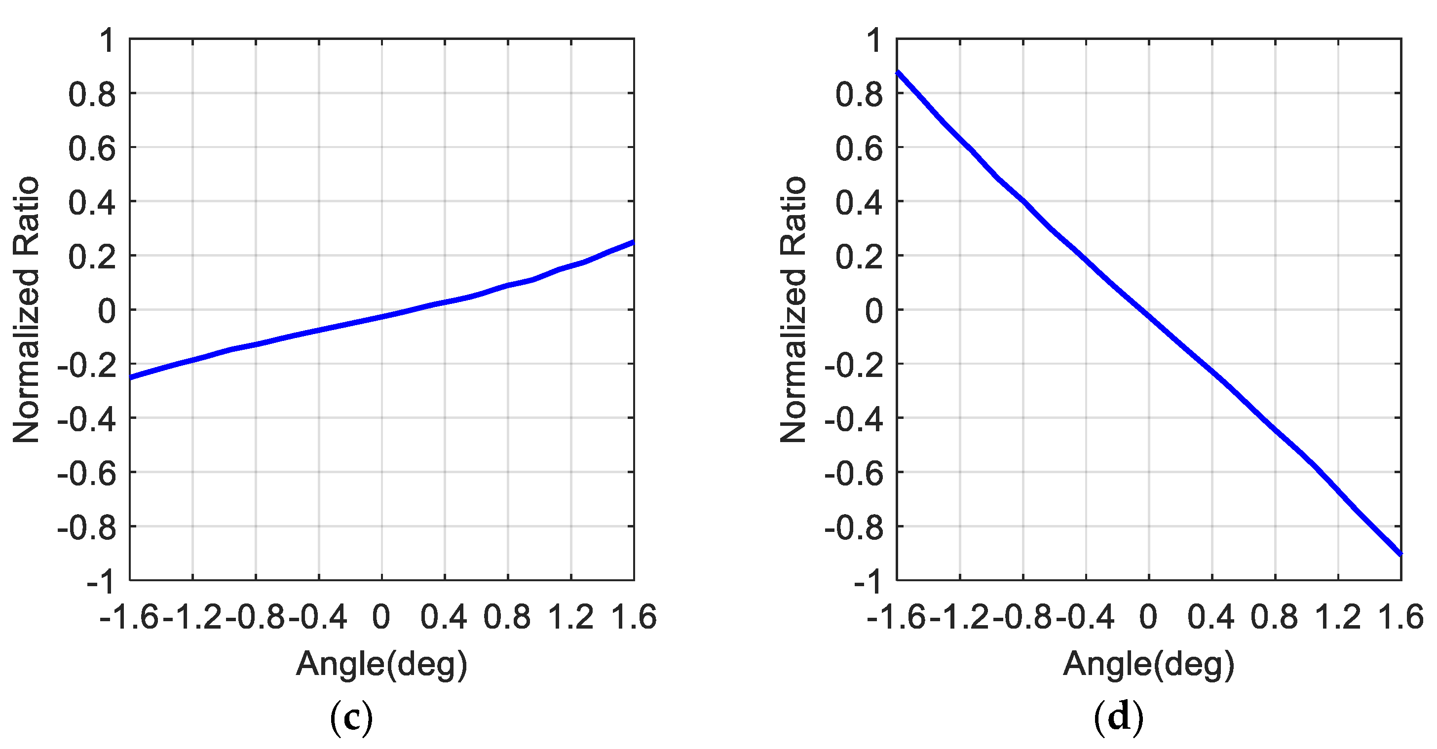
3.2. Target Relocation by Exploiting the Antenna Pattern Information

As mentioned above, both the amplitude errors ( A 1 and A 2 ) and the phase errors ( φ 1 and φ 2 ) determine the channel mismatch. Accordingly, it is quite essential to estimate the amplitude and phase error to mitigate the channel mismatch. However, it is difficult to simultaneously estimate four unknowns (i.e., A 1 , A 2 , φ 1 , and φ 2 ) with limited prior information.
Fortunately, we mainly concern the monopulse ratio between the difference channel and the sum channel. The comprehensive effect of the amplitude error A i and the phase error φ i can be modeled as K ^ and φ ^ , where K ^ and φ ^ denote the initial MPC result and channel mismatch phase error, respectively. For the purpose of analysis, (23) is simplified as
K = K ^ e j φ ^
where K ^ = A ^ Δ / A ^ Σ , A ^ Δ = ( 1 A 2 / A 1 cos ( φ ) ) 2 + ( A 2 / A 1 sin ( φ ) ) 2 , A ^ Σ = ( 1 + A 2 / A 1 cos ( φ ) ) 2 + ( A 2 / A 1 sin ( φ ) ) 2 ,
φ ^ = atan ( A 2 / A 1 sin ( φ ) 1 A 2 / A 1 cos ( φ ) ) atan ( A 2 / A 1 sin ( φ ) 1 + A 2 / A 1 cos ( φ ) )
Based on the above simplification, we convert the problem of estimating A 1 , A 2 , φ 1 , and φ 2 into estimating K ^ and φ ^ , and the number of unknowns is cut in half.
As illustrated in (21) and (23), it is the reason that the leaked energy of the real part degrades the performance of DOA (i.e., GMTR). Therefore, we mainly concern the effect of the channel mismatch phase error φ ^ . Then, channel mismatch can be eliminated if the channel mismatch phase error φ ^ is well compensated.
In order to concentrate all the energy of MPC to the imaginary part, a channel mismatch phase error compensation factor φ c o m is constructed. By performing the phase compensation by multiplying (23) with this channel mismatch phase error compensation factor, we can obtain
K = K ^ e j φ ^ × e j φ c o m
The phase constraint of the channel mismatch phase error compensation factor φ c o m can be given by
min φ c o m φ ^ + φ c o m 2 = π 2 + 2 k π
Equation (25) guarantees that the main energy is not leaked to the real part and mainly concentrates on the imaginary part of the KA-MPC.
The real monopulse curve for the airborne radar can be measured based on the antenna pattern information in the microwave anechoic chamber (see Figure 4), and the ideal monopulse curve can be computed with the antenna geometry configuration (see Figure 2). Therefore, the channel mismatch phase error compensation factor φ c o m can be estimated with the least squares (LS) method. By exploiting the antenna pattern information, the knowledge aided MPC (KA-MPC) can be acquired. Then, the final phase term in KA-MPC satisfies
φ ^ f = φ ^ + φ c o m = π 2 + 2 k π , k Z
where φ ^ f is the final phase factor after phase compensation. In the ideal conditions, φ c o m is equal to zero (i.e., φ c o m = 0 ).
In the non-ideal conditions, Equation (26) still holds since we can estimate and adjust the channel phase compensation term φ c o m .
After some simplification, the final KA-MPC can be expressed as
K = j K ^ = j A ^ Δ A ^ Σ
It can be seen from the above analysis that the KA-MPC in (27) and the ideal MPC in (14) have similar forms, which means that the energy is mainly concentrated on the imaginary part of the KA-MPC.
By exploiting the KA-MPC, the azimuth offset of the potential target in KA-GMTR can be given by
δ θ = λ π D cos θ c arctan ( K im ) tan θ c
where K im is the imaginary part of K .
For a potential target, it may be illuminated by multiple beams with the antenna. In the process of GMTR, it may be relocated multiple times with respect to different antenna beam boresights. When the slope of the MPC is not correct, it is difficult to relocate the potential targets to the same position, and ghost targets may occur on the imaging map. In this case, false-alarm targets are just ghost ones of the real targets. However, with the accurate KA-MPC, this phenomenon may be overcome, and the potential targets will be relocated on the same azimuth positions even though they are illuminated by multiple beams. An illustration of this phenomenon is shown in Figure 5.
Figure 5 shows a schematic diagram of ground moving target relocation with three adjacent beams. In Figure 5, one target is illuminated three times by the antenna beam, and three azimuth offsets are estimated, with respect to the three beam boresights. The target is relocated on the three azimuth geometry locations based on the conventional GMTR method in Figure 5a, while it is relocated on the same azimuth geometry locations based on KA-GMTR in Figure 5b. This is because the MPC is not correct in conventional GMTR, and the distorted MPC can hardly integrate the three relocation results from three beams to the same azimuth geometry position. However, the KA-MPC is accurate and robust to channel mismatch in real conditions, and it can easily integrate the three relocation results to the same azimuth geometry position. Finally, the detailed processing flowchart of the proposed KA-GMTR algorithm is summarized in Figure 6.

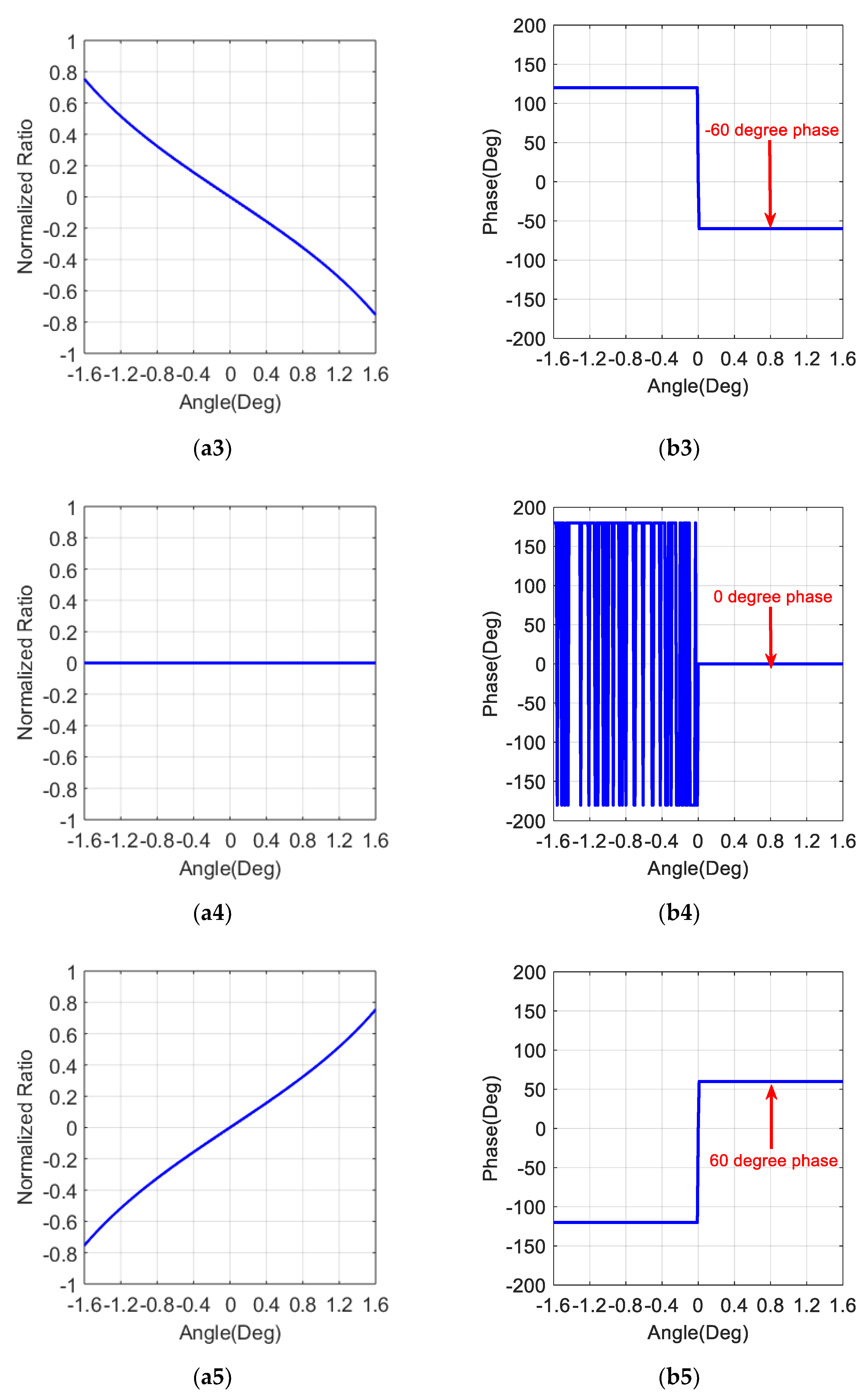
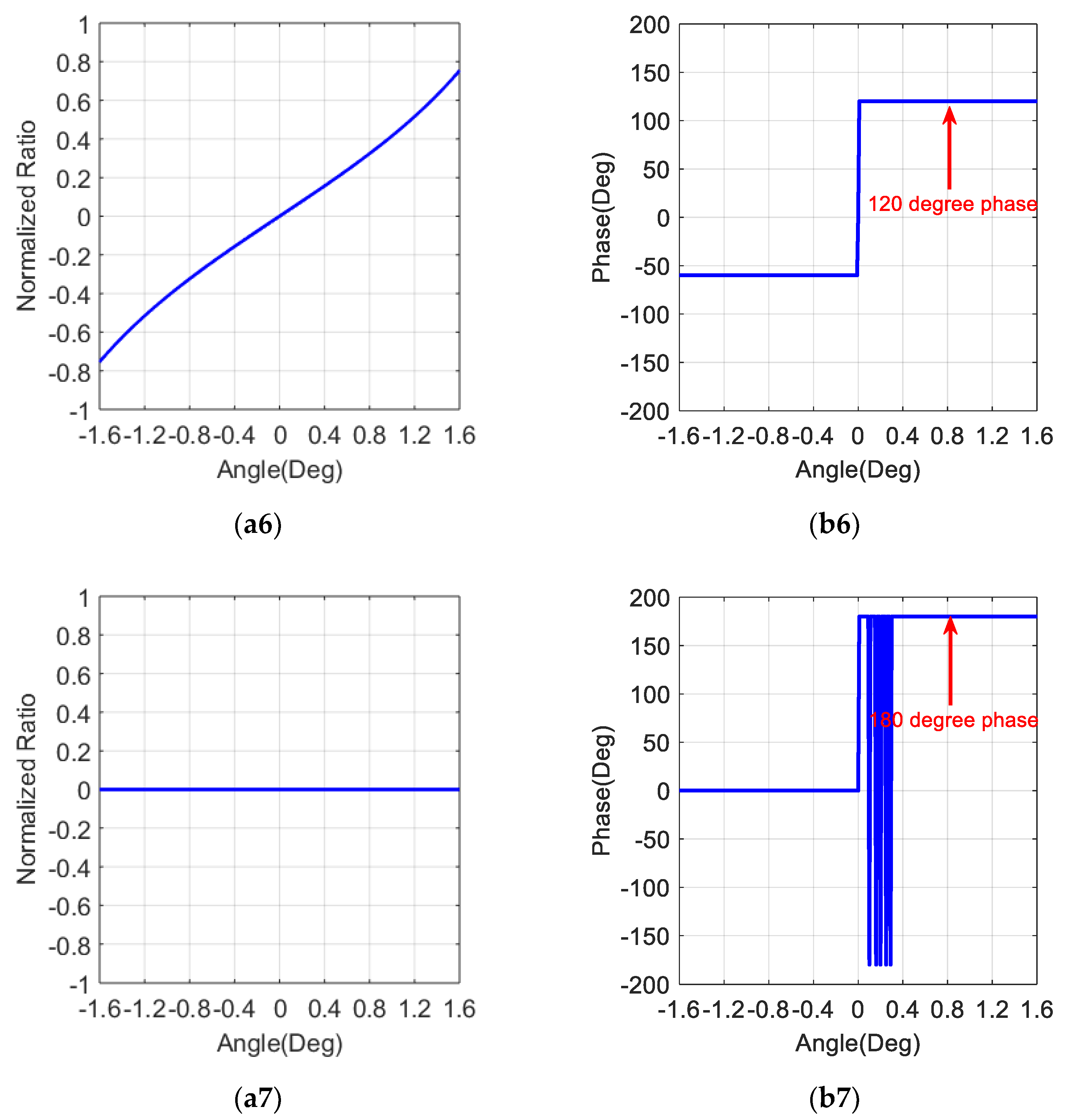
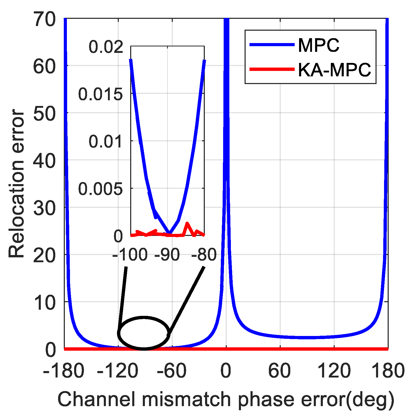
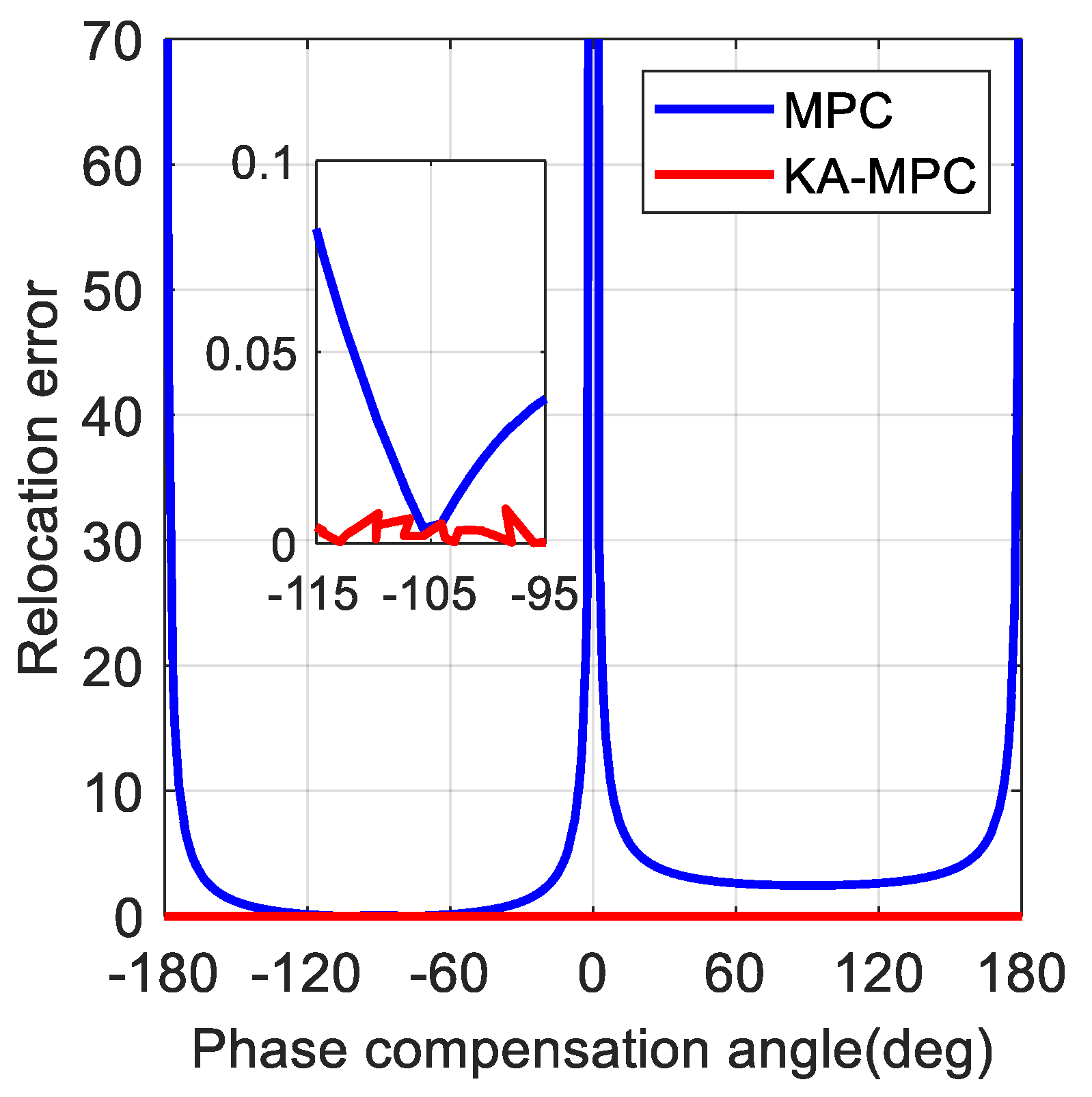
3.3. Performance of Target Relocation

In this section, the accuracy of the azimuth offset estimation (i.e., the target relocation) will be analyzed. For the same MPC ratio value Ω , the estimated azimuth offset with respect to the boresight can be estimated as
δ θ 1 = Ω K 1
δ θ 2 = Ω K 2
where δ θ 1 and δ θ 2 are the estimated azimuth offsets of the conventional MPC and the KA-MPC, respectively. K 1 and K 2 denote the slope of the conventional MPC and the KA-MPC, respectively. Then, the target relocation error of these two MPCs can be computed as
Δ δ = | δ θ 1 δ θ 2 | = Ω | 1 K 1 1 K 2 |
Assuming that the final channel phase angles of the two MPCs are α and β , the slopes of these two channel phase angles correspond to K 1 and K 2 , respectively.
The absolute value of the KA-MPC can be given by
K m = | A ^ Δ A ^ Σ |
Then, we can obtain the relation between the imaginary part of the MPC and the absolute value of the KA-MPC as
K 1 = K m sin α
K 2 = K m sin β
Equation (31) can be simplified as
Δ δ = Ω K m | 1 sin ( α ) 1 sin ( β ) | = Ω K m | sin ( β ) sin ( α ) sin ( α ) sin ( β ) |
According to the trigonometric formula, we can obtain the following equation
Δ δ = Ω K m | 2 cos ( β + α 2 ) sin ( β α 2 ) sin ( α ) sin ( β ) |
Since the slope angle is very small for conventional MPC in real conditions due to channel mismatch, the final channel phase angle α may be equal to zero (i.e., α 0 ) in some extreme cases. In this case, the azimuth offset based on the conventional MPC is infinite, which is given by
lim α 0 δ θ 1 = lim α 0 Ω K m sin ( α ) =
The maximum relocation error between the proposed KA-GMTR and the conventional GMTR can be calculated as
lim α 0 Δ δ = lim α 0 Ω K m | 2 cos ( β + α 2 ) sin ( β α 2 ) sin ( α ) sin ( β ) | =
From (37) and (38), we know that the GMTR performance degrades greatly with the decrease of the slope in conventional MPC, and the azimuth offset may hardly be estimated in some extreme cases.
Figure 7 gives the relocation error curve with different channel mismatch phase errors. The white Gaussian noise with zero mean and covariance 1 is added in this simulation. The different channel mismatch phase errors can be used to simulate the different channel mismatch scenes.
From Figure 7, we can see that the target relocation error based on conventional MPC has a minimum when the channel mismatch phase error is equal to −90 degrees. When the channel mismatch phase error is greater than or less than −90 degrees, the target relocation error increases. This is because the imaginary part of the conventional MPC curve has the largest slope, and this trend is consistent with Figure 4. However, the target relocation error based on KA-MPC is small, which means that the KA-MPC is robust when channel mismatch occurs. Therefore, the KA-MPC can be used to relocate the potential targets.

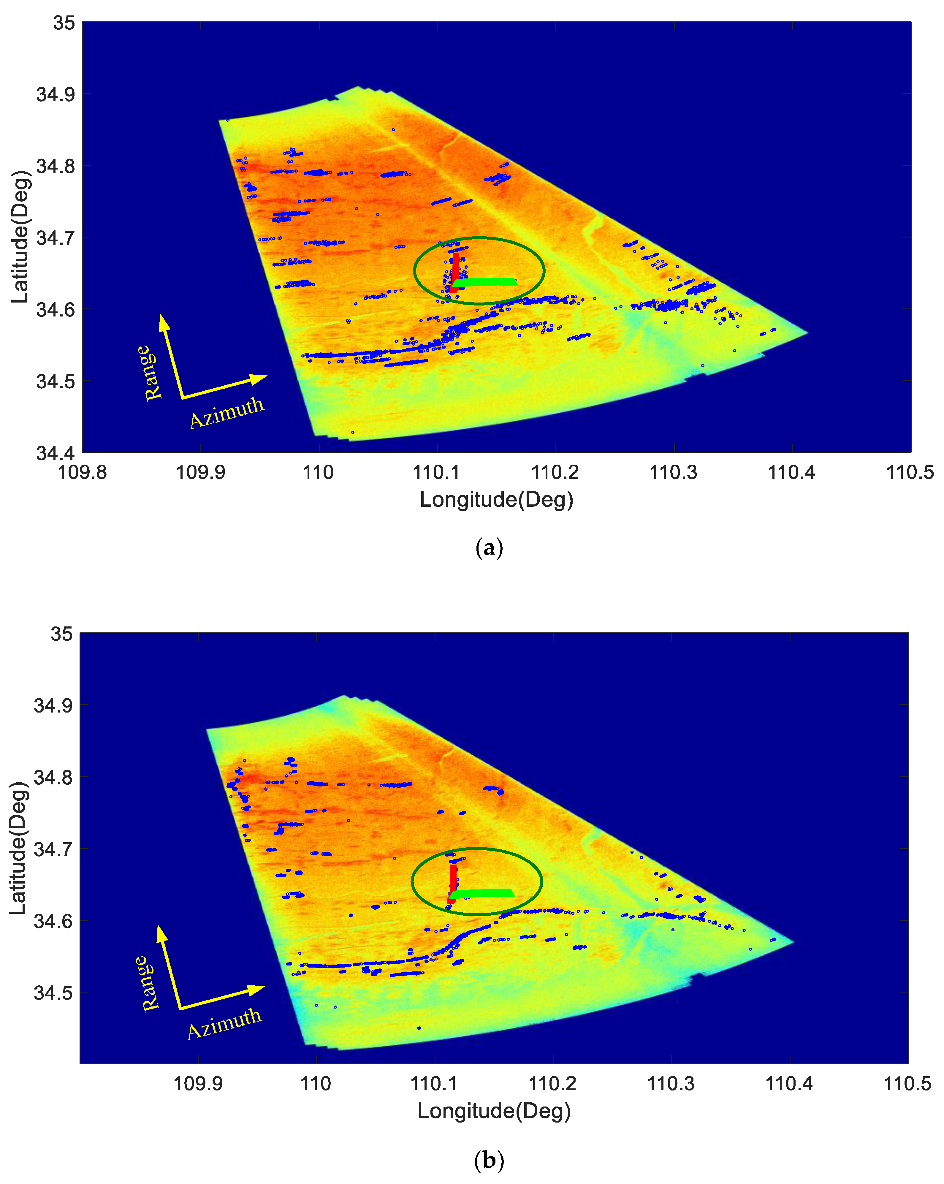
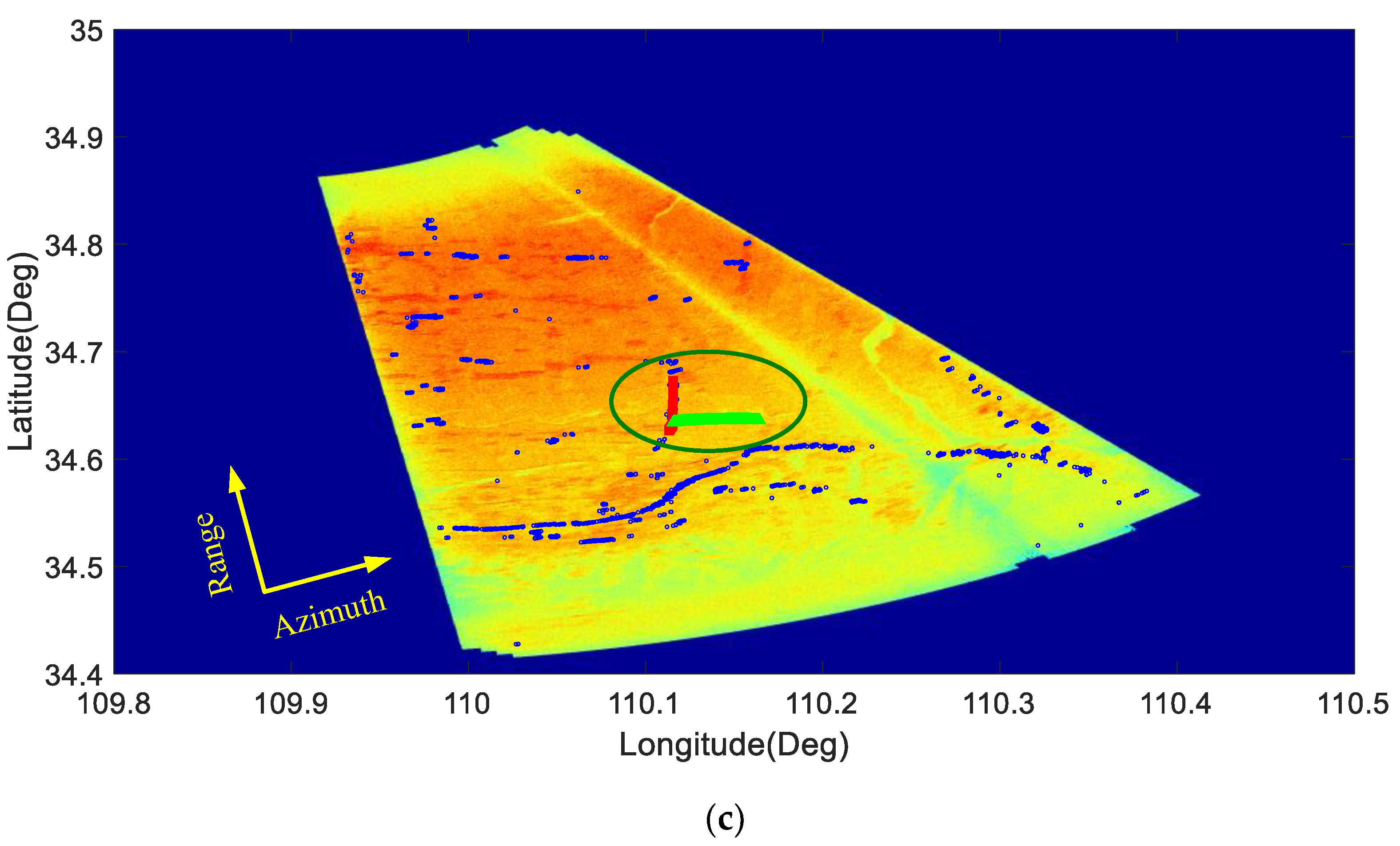
4. Real Data Results

In this section, the performance of KA-GMTR will be investigated using airborne real-measured datasets. All these real-measured data were collected with WAS-GMTI mode.

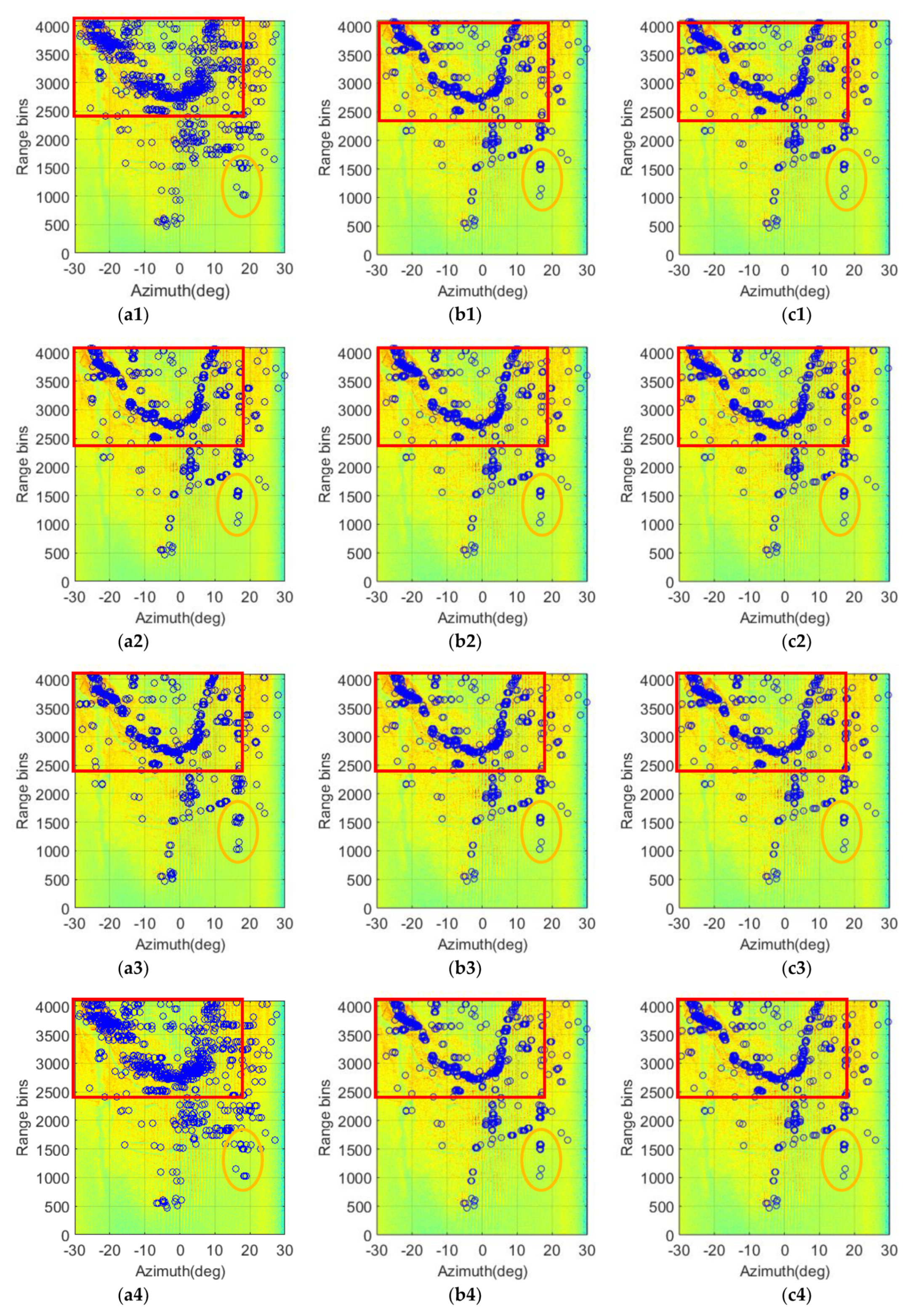
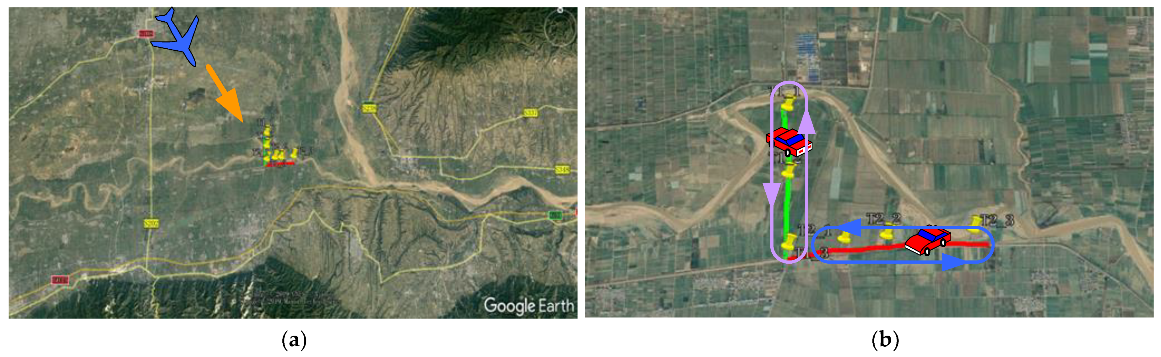
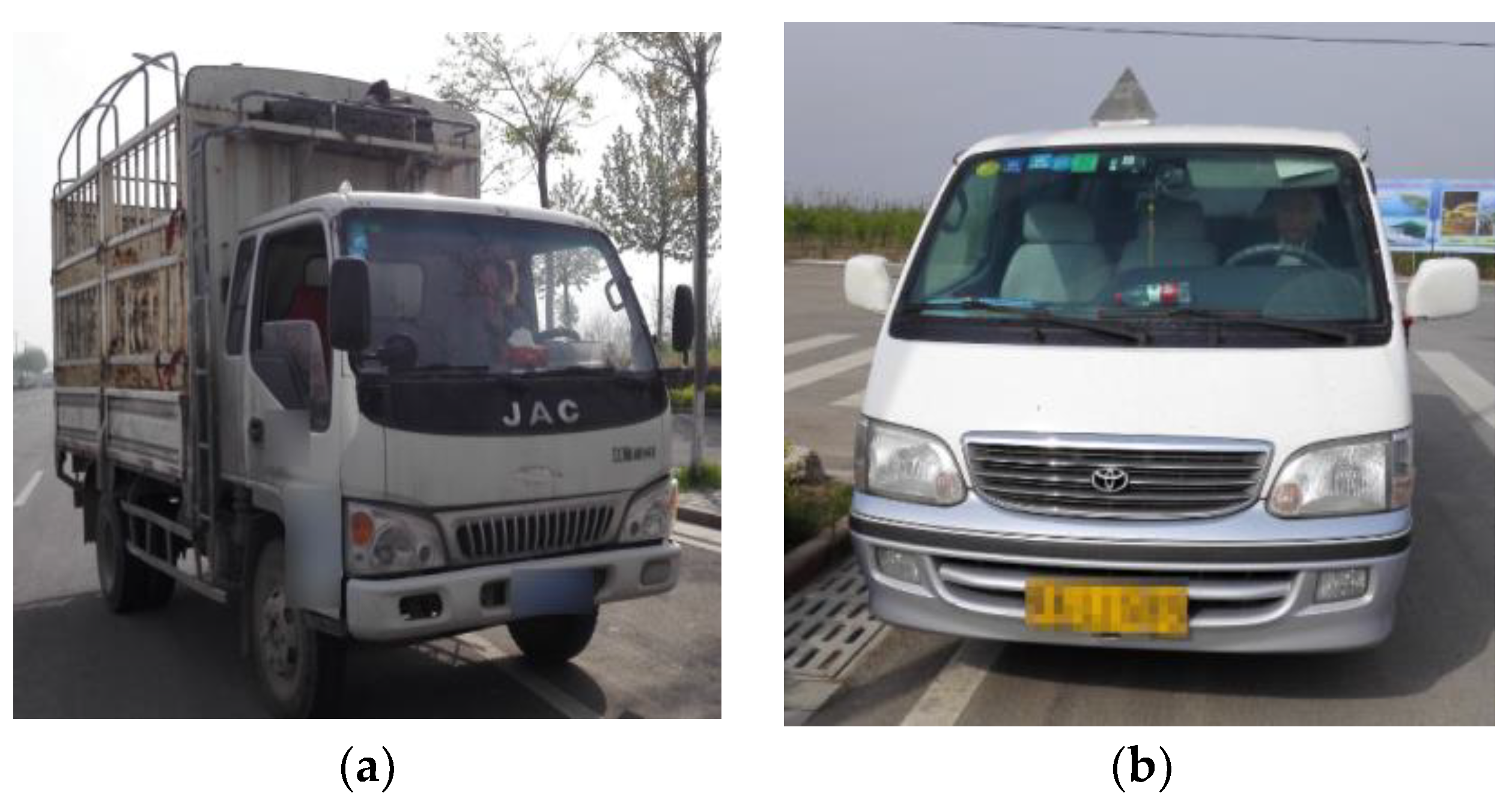
4.1. Experimental Results I

The first real-measured dataset is collected by airborne radar. The main parameters for the airborne radar are listed in Table 1.
Figure 8 gives a comparison result of the conventional MPC before and after channel mismatch phase error compensation. As shown in Figure 8a, the channel mismatch phase error φ ^ is about 15 degrees. Plenty of energy leaks to the real part, which makes the slope very small in the conventional MPC in Figure 8c. It is hard to estimate the azimuth offset and relocate the potential target. Figure 8b shows the phase of the KA-MPC result after channel mismatch phase error compensation. We can observe that little energy is leaked into the real part, and the slope is very large in KA-MPC in Figure 8d. From Figure 8d, we also know that the slope of the KA-MPC is larger than that of the conventional MPC. The large slope is quite significant to relocate the potential targets in the process of GMTR. Figure 9 gives the target relocation error with different channel mismatch phase error compensation factors.
From Figure 9, it can be seen that the target relocation error curve with conventional MPC is close to zero when the channel mismatch phase error compensation factor is about −105 degrees. This is because the final phase angle of the MPC is −90 degrees due to the superposition of the channel mismatch phase error compensation factor and the initial channel mismatch phase error (i.e., −15 degrees). The target relocation error curve has peaks when the channel mismatch phase error compensation factors are near −195, −15, and 165 degrees, respectively. This is because the slope of the imaginary part in the MPC is very small, and the target cannot be well relocated. However, the target relocation error curve with KA-MPC is always small, which means that KA-MPC performs robustly when the channel mismatch phase error varies.

4.2. Experimental Results II

In this section, the airborne results are provided to validate the effectiveness of the proposed KA-GMTR algorithm.
Figure 10 lists the target relocation results for conventional GMTR, Direct KA-GMTR (DKA-GMTR) [50], and the proposed KA-GMTR. For the sake of clarity, the relocation results are transformed into the Range-Doppler domain. The detailed DBS imaging method and the DBS stitching method can be found in [59,60]. From Figure 10a, we can see that the potential targets are not relocated on the main lobe of the DBS image after GMTR operation, and the relocated places deviate from the center of the imaging scene. However, the potential targets are relocated more concentrated to the main lobe of the DBS image in Figure 10b,c. Three of the same patches are masked with ellipse in Figure 10. Especially for region #3, we find that the relocated potential target in Figure 10c is closer to the main lobe of the DBS image than the relocated one in Figure 10a,b.
For multiple beams, the potential targets may be relocated many times when it is illuminated by multiple beams in the scanning operation of the antenna. The relocated azimuth position will be in the same position if the relocation method is accurate. In order to make a clear comparison between GMTR, DKA-GMRR, and the proposed KA-GMTR, the target’s relocation results with multiple beams ranged from −30 degrees to 30 degrees are stitched together to form the target tracks. The tracks of the potential targets with different GMTR methods are given in Figure 11. For the sake of fairness, the EFA based STAP clutter suppression operation [12] and Cell Averaging CFAR (CA-CFAR) processing operation [1,2,61,62] are adopted with the same parameter in our experiments. Therefore, the input data for both target relocation methods are the same.
As shown in Figure 11a, it is obvious that the tracks of the relocated targets are heavily spread in the azimuth direction (see the red rectangle), and lots of ghost targets blur the real tracks. These ghost targets may be the mirrors of the same target, which are generated by multiple beams when they are performed by GMTR operation. Obviously, these distributed ghost targets increase false alarms and blur the target tracks. By contrast, a small azimuth bias can be found in Figure 11b,c (see the red rectangle). Moreover, the track of the relocated targets in Figure 11c is more concentrated in the azimuth direction than those in Figure 11a,b. This means that the number of the ghost targets is decreased in the proposed KA-GMTR method.
For detailed analysis, two patches for the same regions are marked out with ellipses in Figure 11; it can be seen that there are many ghost targets in Figure 11a while the ghost targets are eliminated in Figure 11b,c (see the orange ellipse). Since the four potential targets are illuminated by at least two beams with the antenna, the four targets will be relocated by two times. The two relocated azimuth positions are not the same in the conventional GMTR method due to channel mismatch. For KA-GMTR, the four potential targets are nearly relocated on the same azimuth positions because the channel mismatch is well compensated using the antenna pattern information. Moreover, the proposed KA-GMTR method provides better target relocation performance compared with the DKA-GMTD method. This can be explained that the boresight angle in KA-MPC is compensated with higher accuracy than that in the DKA-MPC for the phased array radar. In the following experiment, its effectiveness in different cases of channel mismatch will be demonstrated.

4.3. Experimental Results III

As mentioned in Section 3, channel mismatch is the main factor that degrades the target relocation performance. To further verify the robustness of the proposed method, an experiment for target relocation under different cases of channel mismatch is carried out. The different channel mismatch phase error factors φ 0 are added to the receiving sum channel and difference channel to simulate the different cases of channel mismatch. It should be noted that the initial channel mismatch phase error φ i n i in the real-measured data is about 15 degrees. Table 1 gives the main radar parameters. The target relocation results under different channel mismatch phase error factors with conventional GMTR method and the proposed KA-GMTR method are given in Figure 12.
In Figure 12, the first column is the target relocation results obtained by the conventional GMTR method under the channel mismatch phase errors −180, −120, −60, 0, 60, 120, and 180 degrees, respectively. The second column corresponds to the DKA-GMTR method under these different channel mismatch phase error factors. The third column corresponds to the proposed KA-GMTR method under these different channel mismatch phase error factors. The different channel phase compensator factors can be seen as the different cases of channel mismatch. The closer to 180, 0, or 180 degrees the absolute phase difference | φ i n i + φ 0 | is, the more serious the channel mismatch is. From the first column of Figure 12, it is obvious that the tracks of the potential targets are heavily spread in the azimuth direction with the variation of the absolute phase value | φ i n i + φ 0 | , and the tracks under the channel phase error factors −180, 0, and 180 degrees are the most blurred among all the tracks. This phenomenon may be explained by the fact that the synthetic phase difference between the sum and difference channel is close to 0 or 180 degrees, which makes the slope of the imaginary part in the conventional MPC very small. Accordingly, the target relocation performance degrades greatly in these three cases. When the channel mismatch phase error is equal to −120 degrees, the channel mismatch phase error φ i n i is superposed with the added channel mismatch phase error. In this case, the synthetic phase angle of the MPC is −105 degrees, which is quite close to ideal conditions. Accordingly, as shown in Figure 12a, the conventional GMTR method only performs well when the channel mismatch phase error is −120 degrees. However, it can be seen that all the tracks of the potential targets are concentrated in the second column and the third column of Figure 12 (see the red rectangle and the orange ellipse). Moreover, the track in the third column seems more concentrated than that in the second column. On the one hand, the channel mismatch is well compensated in different channel mismatch situations in the proposed KA-GMTR; on the other hand, the boresight angle is accurately compensated in the phased array radar. Therefore, the proposed KA-GMTR is more robust than the conventional GMTR and DKA-GMTR under channel mismatch conditions. Based on this experiment, the proposed KA-GMTR method is more robust in the case of channel mismatch.
As illustrated above, after clutter suppression and CFAR processing, the number of potential targets is mainly determined by the relocation accuracy. An accurate relocation method will relocate the same target on the same azimuth positions, even if it is illuminated or relocated many times with respect to many beams. To the contrary, if the relocation accuracy is not accurate, one target may be relocated on many azimuth positions, and false alarms will occur. Therefore, the relocated number of potential targets can be utilized to evaluate the performance of different target relocation methods. The number of the relocated targets under different channel mismatch phase error factors with these two methods is shown in Figure 13.
Figure 13 shows the curve of the number of targets under different channel mismatch phase errors for three GMTR methods. We found that the curve of the conventional GMTR method flutters heavily. It has a bottom of −120 degrees and peaks at −180, 0, and 180 degrees. The number of potential targets of DKA-GMTR and the proposed KA-GMTR remains stable. Moreover, the proposed KA-GMTR has the lowest target number, which demonstrates that KA-GMTR is robust to channel mismatch phase errors. It is worth mentioning that the trend of potential target numbers after GMTR operation is in accordance with the trend of target relocation error in “Experimental Results I”. The effectiveness and robustness of the proposed KA-GMTR are adequately demonstrated by the contrast experiments.

4.4. Experimental Results IV

In this part, to demonstrate the practicability of the proposed algorithm, the other airborne dual-channel real data are applied. The detailed information of the airborne radar is listed in Table 2.
The corresponding optical image from Google Earth Map of the airborne experimental results is shown in Figure 14. The data acquisition time is a little later than the picturing time in Google Earth Map. The track of the cooperative target T1 is marked with green color, while the cooperative target T2 is with red color. A zoomed in result of the two cooperative targets is given in Figure 14b. The track of the cooperative target T1 is marked with three typical positions (i.e., T1_1, T1_2, and T1_3) to illustrate the movement of T1, and T2 is marked with three typical positions (i.e., T2_1, T2_2, and T2_3) to illustrate its movement. From Figure 14b, we can see that the two cooperative targets are mainly moving on the village road.
The two cooperative targets are shown in Figure 15, and both of them are travelling back and forth on the village road. The velocity of the two cooperative targets is less than 50 km/h in this experiment.
Figure 16 shows the results of the relocated targets on the DBS image using different GMTR methods. In Figure 16a, it can be observed that the detected targets deviate from the roads in the azimuth direction in the conventional GMTR method. However, the detected targets are well relocated on the roads in the KA-GMTR method in Figure 16b,c. Moreover, the distribution of the potential targets based on the conventional GMTR method is wider than that of the DKA-GMTR and KA-GMTR method in the azimuth direction (i.e., longitude). The tracks of the relocated targets in Figure 16c are also thinner and more concentrated than that of the ones in Figure 16b. This is because the channel mismatch is inevitable in practice, and the channel mismatch property degrades the target relocation performance in the conventional GMTR method. However, the channel mismatch and boresight angle are well compensated before performing target relocation operation in KA-GMTR. Therefore, the proposed KA-GMTR algorithm can still maintain high target relocation accuracy under the channel mismatch scenarios. Comparisons of the zoomed-in views for the same region are given in Figure 17.
From Figure 17, a phenomenon can be found that shows the distribution range of the cooperative target T1 is larger than that of T2. This is because T1 is moving towards the radar with a high radial velocity, and T2 is moving in the cross-track direction of the airplane with a small radial velocity. A high radial velocity is corresponding to a high Doppler shift. By exploiting the antenna pattern information, the channel mismatch can be well estimated and compensated, and the accuracy of the azimuth offsets (i.e., the target relocation) is greatly improved in the DKA-GMTR method and the proposed KA-GMTR method. As shown in Figure 17, the cooperative targets T1 and T2 are better relocated on the village roads in the proposed KA-GMTR method than of that in the DKA-GMTR method. Based on the experimental results, the proposed KA-GMTR method can effectively improve the target relocation accuracy and has good robustness compared with the conventional GMTR method.

5. Conclusions

The advantages of large coverage and high revisit ratio make the airborne wide-area system an attractive tool for surveillance and monitoring. In this paper, an efficient KA-GMTR method for airborne dual-channel wide-area radar is proposed to enhance the target relocation performance and decrease false alarms. The intrinsic reason that degrades the target relocation accuracy is figured out. In order to estimate the channel mismatch error, a KA-MPC is derived by exploiting the prior antenna pattern information. Moreover, the GMTR performance under different channel mismatch errors is analyzed. Finally, the effectiveness and robustness of the proposed KA-GMTR method under the channel mismatch scenarios is verified based on airborne real-data results.
Although four experimental results are conducted in this paper, it will be better if more real experimental datasets be used to verify the proposed KA-GMTR method. Therefore, more airborne experiments will be performed in our future work to demonstrate the robustness of the proposed algorithm. Moreover, we will focus on GMTR performance enhancement with the track information and the road network information in airborne wide-area GMTI applications.

Author Contributions

The research presented in this manuscript was accomplished in collaboration with all of the authors. Conceptualization, H.C. and Z.W.; methodology, H.C. and Z.W.; software, H.C., Z.W., W.G. and H.S.; validation, H.C., Z.W., W.G. and H.S.; formal analysis, H.C.; investigation, H.C. and Z.W.; resources, H.C. and Y.L. (Yaobing Lu); data curation, H.C. and H.S.; writing—original draft preparation, H.C. and Z.W.; writing—review and editing, H.C., Z.W., W.G. and H.S.; visualization, H.C.; supervision, Y.L. (Yaobing Lu) and Y.L. (Yachao Li); project administration, Y.L. (Yaobing Lu) and Y.L. (Yachao Li); funding acquisition, H.C., Y.L. (Yaobing Lu) and Y.L. (Yachao Li). All authors have read and agreed to the published version of the manuscript.

Funding

This work was supported in part by the National Key Research and Development Program of China under Grant 2018YFB2202500, in part by the National Nature Science Foundation of China (NSFC) under Grant 61971042,and in part by the Postdoctoral Science Foundation of China under Grant 2017M610966.

Institutional Review Board Statement

Not applicable.

Informed Consent Statement

Not applicable.

Data Availability Statement

The data presented in this study are available on request from the corresponding author.

Acknowledgments

The authors would like to thank the anonymous reviewers and the associate editor for their valuable comments The authors also would like to thank Jing Liu and Xinmin Wang for their wide support and valuable suggestions.

Conflicts of Interest

The authors declare no conflict of interest.

Appendix A

In this appendix, Equations (8) and (9) are derived. Combining Equations (6) and (7), they can be further expressed as
s Σ = w a ( t t c ) sin c [ B ( τ 2 R 1 c ) ] exp ( j π 2 R 1 + R 2 + R 3 4 R 0 λ ) × [ exp ( j π R 2 R 3 λ ) + exp ( j π R 3 + R 2 λ ) ]
s Δ = w a ( t t c ) sin c [ B ( τ 2 R 1 c ) ] exp ( j π 2 R 1 + R 2 + R 3 4 R 0 λ ) × [ exp ( j π R 2 R 3 λ ) exp ( j π R 3 + R 2 λ ) ]
According to Euler’s formula, Equations (A1) and (A2) can be expressed as
s Σ = 2 cos ( π R 2 R 3 λ ) w a ( t t c ) sin c [ B ( τ 2 R 1 c ) ] exp ( j π 2 R 1 + R 2 + R 3 4 R 0 λ )
s Δ = 2 j sin ( π R 2 R 3 λ ) w a ( t t c ) sin c [ B ( τ 2 R 1 c ) ] exp ( j π 2 R 1 + R 2 + R 3 4 R 0 λ )

Appendix B

In this appendix, Equations (12)–(14) are derived. Substituting (11) into (8) and (9), we can obtain
s Σ = 2 cos ( π D sin θ λ ) w a ( t t c ) sin c [ B ( τ 2 R 1 c ) ] exp ( j π 2 R 1 + R 2 + R 3 4 R 0 λ )
s Δ = 2 j sin ( π D sin θ λ ) w a ( t t c ) sin c [ B ( τ 2 R 1 c ) ] exp ( j π 2 R 1 + R 2 + R 3 4 R 0 λ )
Then, by substituting Equation (11) into Equations (A5) and (A6), the final sum channel signal and the difference channel signal can be denoted as
s Σ = 2 cos ( π D sin ( θ c + δ θ ) λ ) w a ( t t c ) sin c [ B ( τ 2 R 1 c ) ] × exp ( j π 2 R 1 + R 2 + R 3 4 R 0 λ )
s Δ = 2 j sin ( π D sin ( θ c + δ θ ) λ ) w a ( t t c ) sin c [ B ( τ 2 R 1 c ) ] × exp ( j π 2 R 1 + R 2 + R 3 4 R 0 λ )
To simplify Equations (A7) and (A8) further, Equations (12) and (13) can be acquired. Then, by dividing the difference channel signal by the sum channel signal, we can obtain
K = s Δ s Σ = 2 j sin ( π D sin ( θ c + δ θ ) λ ) w a ( t t c ) sin c [ B ( τ 2 R 1 c ) ] × exp ( j π 2 R 1 + R 2 + R 3 4 R 0 λ ) 2 cos ( π D sin ( θ c + δ θ ) λ ) w a ( t t c ) sin c [ B ( τ 2 R 1 c ) ] × exp ( j π 2 R 1 + R 2 + R 3 4 R 0 λ ) = j tan [ π D sin ( θ c + δ θ ) λ ] = j tan [ π D ( sin θ c + cos θ c δ θ ) λ ]

Appendix C

In this appendix, Equations (20) and (21) are derived. By combining Equations (18) and (19), the MPC can be expressed as
K = S ^ Δ S ^ Σ = w a ( t t c ) sin c [ B ( τ 2 R 1 c ) ] × [ A 1 e j φ 1 exp ( j 2 π R 1 + R 2 λ ) A 2 e j φ 2 exp ( j 2 π R 1 + R 3 λ ) ] w a ( t t c ) sin c [ B ( τ 2 R 1 c ) ] × [ A 1 e j φ 1 exp ( j 2 π R 1 + R 2 λ ) + A 2 e j φ 2 exp ( j 2 π R 1 + R 3 λ ) ] = A 1 e j φ 1 exp ( j 2 π R 1 + R 2 λ ) A 2 e j φ 2 exp ( j 2 π R 1 + R 3 λ ) A 1 e j φ 1 exp ( j 2 π R 1 + R 2 λ ) + A 2 e j φ 2 exp ( j 2 π R 1 + R 3 λ ) = 1 A 2 A 1 e j ( φ 2 φ 1 + 2 π R 2 R 3 λ ) 1 + A 2 A 1 e j ( φ 2 φ 1 + 2 π R 2 R 3 λ ) = 1 A 2 A 1 e j ( φ 2 φ 1 + 2 π D s i n θ λ ) 1 + A 2 A 1 e j ( φ 2 φ 1 + 2 π D s i n θ λ )
By using the Euler Formula, Equation (A10) can be transformed as follows
K = 1 A 2 A 1 [ cos ( φ 2 φ 1 + 2 π D s i n θ λ ) + j sin ( φ 2 φ 1 + 2 π D s i n θ λ ) ] 1 + A 2 A 1 [ cos ( φ 2 φ 1 + 2 π D s i n θ λ ) + j sin ( φ 2 φ 1 + 2 π D s i n θ λ ) ] = [ 1 A 2 A 1 cos ( φ 2 φ 1 + 2 π D s i n θ λ ) ] j A 2 A 1 sin ( φ 2 φ 1 + 2 π D s i n θ λ ) [ 1 + A 2 A 1 cos ( φ 2 φ 1 + 2 π D s i n θ λ ) ] + j A 2 A 1 sin ( φ 2 φ 1 + 2 π D s i n θ λ )
Let φ = φ 2 φ 1 + 2 π D s i n θ λ , Equation (A11) is transformed into
K = ( 1 A 2 A 1 cos φ ) j A 2 A 1 sin φ ( 1 + A 2 A 1 cos φ ) + j A 2 A 1 sin φ
Then, Equation (A12) is transformed into
K = ( 1 A 2 A 1 cos φ ) 2 + ( A 2 A 1 cos φ ) 2 ( 1 + A 2 A 1 cos φ ) 2 + ( A 2 A 1 cos φ ) 2 e j [ atan ( A 2 / A 1 sin ( φ ) 1 A 2 / A 1 cos ( φ ) ) atan ( A 2 / A 1 sin ( φ ) 1 + A 2 / A 1 cos ( φ ) ) ]
Let φ ^ = atan ( A 2 / A 1 sin ( φ ) 1 A 2 / A 1 cos ( φ ) ) atan ( A 2 / A 1 sin ( φ ) 1 + A 2 / A 1 cos ( φ ) ) , we can easily obtain Equation (21).

References

  1. Skolnik, M.I. Radar Handbook, 4th ed.; McGraw-Hill: New York, NY, USA, 2008; pp. 23.1–23.36. [Google Scholar]
  2. Richards, M.A. Fundamentals of Radar Signal Processing; McGraw-Hill: New York, NY, USA, 2005. [Google Scholar]
  3. Entzminger, J.N.; Fowler, C.A.; Kenneally, W.J. JointSTARS and GMTI: Past, present and future. IEEE Trans. Aerosp. Electron. Syst. 1999, 35, 748–761. [Google Scholar] [CrossRef]
  4. Ender, J.H.G.; Brenner, A.R. PAMIR-a wideband phased array SAR/ MTI system. IEE Proc.-Radar Sonar Navig. 2003, 150, 165–172. [Google Scholar] [CrossRef] [Green Version]
  5. Brenner, A.; Ender, J. Demonstration of advanced reconnaissance techniques with the airborne SAR/GMTI sensor PAMIR. IEE Proc.-Radar Sonar Navig. 2006, 153, 152–162. [Google Scholar] [CrossRef] [Green Version]
  6. Cerutti-Maori, D.; Klare, J.; Brenner, A.R.; Ender, J.H. Wide-area traffc monitoring with the SAR/GMTI system PAMIR. IEEE Trans. Geosci. Remote Sens. 2008, 46, 3019–3030. [Google Scholar] [CrossRef]
  7. Tanelli, S.; Durden, S.L.; Johnson, M.P. Airborne Demonstration of DPCA for Velocity Measurements of Distributed Targets. IEEE Geosci. Remote Sens. Lett. 2016, 13, 1415–1419. [Google Scholar] [CrossRef]
  8. Ward, J. Space-Time Adaptive Processing for Airborne Radar; MIT Lincoln Lab: Lexington, MA, USA, 1994. [Google Scholar]
  9. Wang, H.; Cai, L. On adaptive spatial-temporal processing for airborne surveillance radar systems. IEEE Trans. Aerosp. Electron. Syst. 1994, 30, 660–670. [Google Scholar] [CrossRef]
  10. Adve, R.S.; Hale, T.B.; Wicks, M.C. Practical joint domain localised adaptive processing in homogeneous and nonhomogeneous environments. Part 1: Homogeneous environments. IEE Proc.-Radar Sonar Navig. 2000, 147, 57–65. [Google Scholar] [CrossRef]
  11. Adve, R.S.; Hale, T.B.; Wicks, M.C. Practical joint domain localised adaptive processing in homogeneous and nonhomogeneous environments. Part 2: Nonhomogeneous environments. IEE Proc.-Radar Sonar Navig. 2000, 147, 66–74. [Google Scholar] [CrossRef] [Green Version]
  12. Tong, Y.L.; Wang, T.; Wu, J.X. Improving EFA-STAP performance using persymmetric covariance matrix estimation. IEEE Trans. Aerosp. Electron. Syst. 2015, 51, 924–936. [Google Scholar] [CrossRef]
  13. Brown, R.D.; Schneible, R.A.; Wicks, M.C.; Wang, H.; Zhang, Y. STAP for clutter suppression with sum and difference beams. IEEE Trans. Aerosp. Electron. Syst. 2000, 36, 634–646. [Google Scholar] [CrossRef]
  14. Yang, Z.; de Lamare, R.C.; Li, X. L1-regularized STAP algorithms with a generalized sidelobe canceler architecture for airborne radar. IEEE Trans. Signal Process. 2012, 60, 674–686. [Google Scholar] [CrossRef]
  15. Fa, R.; de Lamare, R.C.; Wang, L. Reduced-Rank STAP schemes for airborne radar based on switched joint interpolation, decimation and filtering algorithm. IEEE Trans. Signal Process. 2010, 58, 4182–4194. [Google Scholar] [CrossRef] [Green Version]
  16. Sen, S. Low-Rank Matrix Decomposition and Spatio-Temporal Sparse Recovery for STAP Radar. IEEE J. Sel. Top. Signal Process. 2015, 9, 1510–1523. [Google Scholar] [CrossRef]
  17. Duan, K.Q.; Xu, H.; Yuan, H.D.; Xie, H.T.; Wang, Y.L. Reduced-DOF Three-Dimensional STAP via Subarray Synthesis for Nonsidelooking Planar Array Airborne Radar. IEEE Trans. Aerosp. Electron. Syst. 2020, 56, 3311–3325. [Google Scholar] [CrossRef]
  18. Steiner, M.; Gerlach, K. Fast converging adaptive processor or a structured covariance matrix. IEEE Trans. Aerosp. Electron. Syst. 2000, 36, 1115–1126. [Google Scholar] [CrossRef]
  19. Abramovich, Y.I.; Besson, O. Regularized covariance matrix estimation in complex elliptically symmetric distributions using the expected likelihood approach—Part 1: The over-sampled case. IEEE Trans. Signal Process. 2013, 61, 5807–5818. [Google Scholar] [CrossRef] [Green Version]
  20. Aubry, A.; de Maio, A.; Pallotta, L. A Geometric Approach to Covariance Matrix Estimation and its Applications to Radar Problems. IEEE Trans. Signal Process. 2017, 66, 907–922. [Google Scholar] [CrossRef] [Green Version]
  21. De Maio, A.; Pallotta, L.; Li, J.; Stoica, P. Loading Factor Estimation Under Affine Constraints on the Covariance Eigenvalues with Application to Radar Target Detection. IEEE Trans. Aerosp. Electron. Syst. 2018, 55, 1269–1283. [Google Scholar] [CrossRef]
  22. Guerci, J.R.; Baranoski, E.J. Knowledge-aided adaptive radar at DARPA: An overview. IEEE Signal Process. Mag. 2006, 23, 41–50. [Google Scholar] [CrossRef]
  23. Bergin, J.S.; Teixeira, C.M.; Techau, P.M.; Guerci, J.R. Improved clutter mitigation performance using knowledge-aided space-time adaptive processing. IEEE Trans. Aerosp. Electron. Syst. 2006, 42, 997–1009. [Google Scholar] [CrossRef]
  24. Guerci, J.R. Cognitive radar: A knowledge-aided fully adaptive approach. In Proceedings of the IEEE National Conference on Radar, Arlington, VA, USA, 10–14 May 2010; pp. 1365–1370. [Google Scholar] [CrossRef]
  25. Sun, G.C.; Xing, M.D.; Xia, X.-G.; Wu, Y.R.; Bao, Z. Robust Ground Moving-Target Imaging Using Deramp–Keystone Processing. IEEE Trans. Geosci. Remote Sens. 2012, 51, 966–982. [Google Scholar] [CrossRef]
  26. Guo, L.; Deng, W.; Yao, D.; Yang, Q.; Ye, L.; Zhang, X. A Knowledge-Based Auxiliary Channel STAP for Target Detection in Shipborne HFSWR. Remote Sens. 2021, 13, 621. [Google Scholar] [CrossRef]
  27. Li, G.; Xia, X.-G.; Peng, Y.N. Doppler keystone transform: An approach suitable for parallel implementation of SAR moving target imaging. IEEE Geosci. Remote Sens. Lett. 2008, 5, 573–577. [Google Scholar] [CrossRef]
  28. Wang, W.; An, D.X.; Luo, Y.X.; Zhou, Z. M The Fundamental Trajectory Reconstruction Results of Ground Moving Target from Single-Channel CSAR Geometry. IEEE Trans. Geosci. Remote Sens. 2018, 1–11. [Google Scholar] [CrossRef]
  29. Yang, J.; Zhang, Y. An airborne SAR moving target imaging and motion parameters estimation algorithm with azi-muth-dechirping and the second-order keystone transform applied. IEEE J. Sel. Top. Appl. Earth Observ. Remote Sens. 2015, 8, 3967–3976. [Google Scholar] [CrossRef]
  30. Zheng, J.; Zhu, K.; Niu, Z.; Liu, H.; Liu, Q.H. Generalized Dechirp-Keystone Transform for Radar High-Speed Maneuvering Target Detection and Localization. Remote Sens. 2021, 13, 3367. [Google Scholar] [CrossRef]
  31. Zhang, X.; Liao, G.; Zhu, S.; Zeng, C.; Shu, Y. Geometry-Information-Aided Efficient Radial Velocity Estimation for Moving Target Imaging and Location Based on Radon Transform. IEEE Trans. Geosci. Remote Sens. 2014, 53, 1105–1117. [Google Scholar] [CrossRef]
  32. Ender, J.H.G.; Gierull, C.H.; Cerutti-Maori, D. Improved Space-Based Moving Target Indication via Alternate Transmission and Receiver Switching. IEEE Trans. Geosci. Remote Sens. 2008, 46, 3960–3974. [Google Scholar] [CrossRef]
  33. Budillon, A.; Pascazio, V.; Schirinzi, G. Estimation of Radial Velocity of Moving Targets by Along-Track Interferometric SAR Systems. IEEE Geosci. Remote Sens. Lett. 2008, 5, 349–353. [Google Scholar] [CrossRef]
  34. Chapin, E.; Chen, C.W. Airborne along-track interferometry for GMTI. IEEE Aerosp. Electron. Syst. Mag. 2009, 24, 13–18. [Google Scholar] [CrossRef]
  35. Romeiser, R.; Suchandt, S.; Runge, H.; Steinbrecher, U.; Grunler, S. First analysis of TerraSAR-X along-track InSAR-derived current fields. IEEE Trans. Geosci. Remote Sens. 2010, 48, 820–829. [Google Scholar] [CrossRef]
  36. Deming, R.W.; MacIntosh, S.; Best, M. Three-channel processing for improved geo-location performance in SAR-based GMTI interferometry. In Proceedings of the Algorithms for Synthetic Aperture Radar Imagery XIX. International Society for Optics and Photonics, Baltimore, MD, USA, 7 May 2012; p. 8394. [Google Scholar] [CrossRef]
  37. Tian, M.; Yang, Z.W.; Duan, C.D.; Liao, G.S.; Liu, Y.J.; Wang, C.H.; Huang, P.H. A Method for Active Marine Target Detection Based on Complex Interferometric Dissimilarity in Dual-Channel ATI-SAR Systems. IEEE Trans. Geosci. Remote Sens. 2020, 58, 251–267. [Google Scholar] [CrossRef]
  38. Tao, R.; Li, Y.-L.; Wang, Y. Short-Time Fractional Fourier Transform and Its Applications. IEEE Trans. Signal Process. 2010, 58, 2568–2580. [Google Scholar] [CrossRef]
  39. Djurovic, I.; Stankovic, L. Robust Wigner distribution with application to the instantaneous frequency estimation. IEEE Trans. Signal Process. 2001, 49, 2985–2993. [Google Scholar] [CrossRef]
  40. Huang, P.H.; Xia, X.-G.; Gao, Y.S.; Liu, X.Z.; Liao, G.S.; Jiang, X. Ground moving target refocusing in SAR imagery based on RFRT-FrFT. IEEE Trans. Geosci. Remote Sens. 2019, 57, 5476–5492. [Google Scholar] [CrossRef]
  41. Zhu, S.Q.; Liao, G.S.; Qu, Y.; Zhou, Z.G.; Liu, X.Y. Ground Moving Targets Imaging Algorithm for Synthetic Aperture Radar. IEEE Trans. Geosci. Remote Sens. 2010, 49, 462–477. [Google Scholar] [CrossRef]
  42. Li, Z.Y.; Wu, J.J.; Huang, Y.L.; Sun, Z.C.; Yang, J.Y. Ground-moving target imaging and velocity estimation based on mis-matched compression for bistatic forward-looking SAR. IEEE Trans. Geosci. Remote Sens. 2016, 54, 3277–3291. [Google Scholar] [CrossRef]
  43. Li, Y.; Wang, Y.; Liu, B.; Zhang, S.; Nie, L.; Bi, G. A New Motion Parameter Estimation and Relocation Scheme for Airborne Three-Channel CSSAR-GMTI Systems. IEEE Trans. Geosci. Remote Sens. 2019, 57, 4107–4120. [Google Scholar] [CrossRef]
  44. Yang, J.Y.; Qiu, X.L.; Shang, M.Y.; Zhong, L.H.; Ding, C.B. A Method of Marine Moving Targets Detection in Multi-Channel ScanSAR System. Remote Sens. 2020, 12, 3792. [Google Scholar] [CrossRef]
  45. Bergin, J.; Guerci, J.; Kirk, D.; Rangaswamy, M. Site-specific performance gain of optimal MIMO radar in heterogeneous clutter. In Proceedings of the 2018 IEEE Radar Conference (RadarConf18), Oklahoma City, OK, USA, 23–27 April 2018; pp. 1156–1161. [Google Scholar] [CrossRef]
  46. Bergin, J.; Guerci, J.R. Book review of “MIMO radar: Theory and application”. IEEE Aerosp. Electron. Syst. Mag. 2018, 33, 51–53. [Google Scholar] [CrossRef]
  47. Ender, J.H.G. The airborne experimental multi-channel SAR-system AER-II. In Proceedings of the EUSAR’96: European Conference on Synthetic Aperture Radar, Königswinter, Germany, 26–28 March 1996; pp. 49–52. [Google Scholar]
  48. Yan, H.; Wang, R.Y.; Gao, C.G.; Liu, Y.B.; Zheng, M.J.; Deng, Y.K. Channel balancing algorithm in multichannel wide-area surveillance systems. IET Radar Sonar Navig. 2014, 8, 27–36. [Google Scholar] [CrossRef]
  49. Hu, R.; Liu, B.; Wang, T.; Liu, D.; Bao, Z. A Knowledge-Based Target Relocation Method for Wide-Area GMTI Mode. IEEE Geosci. Remote Sens. Lett. 2013, 11, 748–752. [Google Scholar] [CrossRef]
  50. Chen, H.; Lu, Y.; Liu, J.; Yi, X.; Sun, H.; Mu, H.; Wang, Z.; Li, M. Efficient knowledge-aided target relocation algorithm for airborne radar. J. Eng. 2019, 2019, 7589–7592. [Google Scholar] [CrossRef]
  51. Mosca, E. Angle Estimation in Amplitude Comparison Monopulse Systems. IEEE Trans. Aerosp. Electron. Syst. 1969, AES-5, 205–212. [Google Scholar] [CrossRef]
  52. Sherman, S.M. Monopulse Principles and Techniques; Artech House: Norwood, MA, USA, 1984. [Google Scholar]
  53. Paine, A.S. Minimum variance monopulse technique for an adaptive phased array radar. IEE Proc.-Radar Sonar Navig. 1998, 145, 374–380. [Google Scholar] [CrossRef]
  54. Farina, A.; Gabatel, G.; Sanzullo, R. Estimation of target direction by pseudo-monopulse algorithm. Signal Process. 2000, 80, 295–310. [Google Scholar] [CrossRef]
  55. Farina, A.; Gini, F.; Greco, M. DOA estimation by exploiting the amplitude modulation induced by antenna scanning. IEEE Trans. Aerosp. Electron. Syst. 2002, 38, 1276–1286. [Google Scholar] [CrossRef]
  56. Sedehi, M.; Colone, F.; Lombardo, P. Exploiting the joint distribution of amplitude and monopulse ratio for chi-square fluctu-ating targets for target DOA estimation. In Proceedings of the 7th European Radar Conference, Paris, France, 30 September–1 October 2010; pp. 304–307. [Google Scholar]
  57. Nickel, U. Performance analysis of space–time-adaptive monopulse. Signal Process. 2004, 84, 1561–1579. [Google Scholar] [CrossRef]
  58. Nickel, U. Overview of generalized monopulse estimation. IEEE Aerosp. Electron. Syst. Mag. 2006, 21, 27–56. [Google Scholar] [CrossRef]
  59. Chen, H.; Li, M.; Lu, Y.; Wu, Y.A. DBS image stitching algorithm based on affine transformation. In Proceedings of the IET International Radar Conference 2013, Xi’an, China, 14–16 April 2013. [Google Scholar] [CrossRef]
  60. Chen, H.; Li, M.; Wang, Z.; Lu, Y.; Cao, R.; Zhang, P.; Zuo, L.; Wu, Y. Cross-Range Resolution Enhancement for DBS Imaging in a Scan Mode Using Aperture-Extrapolated Sparse Representation. IEEE Geosci. Remote Sens. Lett. 2017, 14, 1459–1463. [Google Scholar] [CrossRef]
  61. Guan, J.; Peng, Y.-N.; He, Y.; Meng, X.-W. Three types of distributed CFAR detection based on local test statistic. IEEE Trans. Aerosp. Electron. Syst. 2002, 38, 278–288. [Google Scholar] [CrossRef]
  62. Ghosh, R.; Vajpeyi, A.; Akula, A.; Shaw, V.; Kumar, S.; Sardana, H.K. Performance Evaluation of a Real-Time Seismic Detection System Based on CFAR Detectors. IEEE Sens. J. 2020, 20, 3678–3686. [Google Scholar] [CrossRef]
Figure 1. Geometry of airborne dual-channel GMTI.
Remotesensing 13 04724 g001
Figure 2. Illustration of airborne dual-channel radar system. (a) Ideal receiving antenna pattern (single way). (b) Ideal sum and difference signals. (c) Ideal MPC.
Remotesensing 13 04724 g002
Figure 3. Illustration of channel mismatch for dual-channel radar system. (a) Ideal dual-channel radar system. (b) Real dual-channel radar system with channel mismatch.
Remotesensing 13 04724 g003
Figure 4. Comparisons of MPC under different channel mismatch phase errors. (a1) Imaginary part of the MPC for the scene of −180-degree channel mismatch phase error. (b1) Phase of the MPC for the scene of −180-degree channel mismatch phase error. (a2) Imaginary part of the MPC for the scene of −120-degree channel mismatch phase error. (b2) Phase of the MPC for the scene of −120-degree channel mismatch phase error. (a3) Imaginary part of the MPC for the scene of −60-degree channel mismatch phase error. (b3) Phase of the MPC for the scene of −60-degree channel mismatch phase error. (a4) Imaginary part of the MPC for the scene of 0-degree channel mismatch phase error. (b4) Phase of the MPC for the scene of 0-degree channel mismatch phase error. (a5) Imaginary part of the MPC for the scene of 60-degree channel mismatch phase error. (b5) Phase of the MPC for the scene of 60-degree channel mismatch phase error. (a6) Imaginary part of the MPC for the scene of 120-degree channel mismatch phase error. (b6) Phase of the MPC for the scene of 120-degree channel mismatch phase error. (a7) Imaginary part of the MPC for the scene of 180-degree channel mismatch phase error. (b7) Phase of the MPC for the scene of 180-degree channel mismatch phase error.
Remotesensing 13 04724 g004aRemotesensing 13 04724 g004bRemotesensing 13 04724 g004c
Figure 5. Illustration of ground moving target relocation. (a) Conventional GMTR. (b) KA-GMTR.
Remotesensing 13 04724 g005
Figure 6. Flowchart of the proposed KA-GMTR algorithm.
Remotesensing 13 04724 g006
Figure 7. Relocation error with different channel mismatch phase errors.
Remotesensing 13 04724 g007
Figure 8. Comparison of MPC before and after channel mismatch phase error compensation. (a) Phase of conventional MPC. (b) Phase of KA-MPC. (c) Normalized radio of conventional MPC. (d) Normalized radio of KA-MPC.
Remotesensing 13 04724 g008aRemotesensing 13 04724 g008b
Figure 9. Target relocation error with different channel mismatch phase error compensation factors.
Remotesensing 13 04724 g009
Figure 10. Comparisons of different target relocation methods. (a) Conventional GMTR method. (b) DKA-GMTR method. (c) Proposed KA-GMTR method.
Remotesensing 13 04724 g010
Figure 11. Comparisons of different target relocation methods. (a) Conventional GMTR method. (b) DKA-GMTR method. (c) Proposed KA-GMTR method.
Remotesensing 13 04724 g011
Figure 12. Comparisons of different target relocation methods. (a1) Conventional GMTR method under the channel mismatch phase error −180 degrees. (b1) DKA-GMTR method under the channel mismatch phase error −180 degrees. (c1) Proposed KA-GMTR method under the channel mismatch phase error −180 degrees. (a2) Conventional GMTR method under the channel mismatch phase error −120 degrees. (b2) DKA-GMTR method under the channel mismatch phase error −120 degrees. (c2) Proposed KA-GMTR method under the channel mismatch phase error −120 degrees. (a3) Conventional GMTR method under the channel mismatch phase error −60 degrees. (b3) DKA-GMTR method under the channel mismatch phase error −60 degrees (c3) Proposed KA-GMTR method under the channel mismatch phase error −60 degrees. (a4) Conventional GMTR method under the channel mismatch phase error 0 degree. (b4) DKA-GMTR method under the channel mismatch phase error 0 degree (c4) Proposed KA-GMTR method under the channel mismatch phase error 0 degree. (a5) Conventional GMTR method under the channel mismatch phase error 60 degrees. (b5) DKA-GMTR method under the channel mismatch phase error 60 degrees (c5) Proposed KA-GMTR method under the channel mismatch phase error 60 degrees. (a6) Conventional GMTR method under the channel mismatch phase error 120 degrees. (b6) DKA-GMTR method under the channel mismatch phase error 120 degrees (c6) Proposed KA-GMTR method under the channel mismatch phase error 120 degrees. (a7) Conventional GMTR method under the channel mismatch phase error 180 degrees. (b7) DKA-GMTR method under the channel mismatch phase error 180 degrees. (c7) Proposed KA-GMTR method under the channel mismatch phase error 180 degrees.
Remotesensing 13 04724 g012aRemotesensing 13 04724 g012b
Figure 13. Curve number of targets with different channel mismatch phase error.
Remotesensing 13 04724 g013
Figure 14. Google Earth map of the airborne experiments. (a) Google Earth map for the imaging scene. (b) Track of the cooperative targets for this experiment.
Remotesensing 13 04724 g014
Figure 15. Cooperative vehicle targets of the experiments. (a) Truck. (b) Microbus.
Remotesensing 13 04724 g015
Figure 16. Comparisons of different target relocation methods. (a) Conventional GMTR method. (b) DKA-GMTR method. (c) Proposed KA-GMTR method.
Remotesensing 13 04724 g016aRemotesensing 13 04724 g016b
Figure 17. Zoomed-in results of different target relocation methods. (a) Conventional GMTR method. (b) DKA-GMTR method. (c) Proposed KA-GMTR method.
Remotesensing 13 04724 g017
Table 1. Parameters used in the experiments.
ParametersValuesParametersValues
Band width50 MHzTime width62.5 us
Platform50 m/sMeanslant range10 km
Range numbers4096Scanning area−30~30°
Pitching angle10°Beam width
Table 2. Parameters used in the experiments.
ParametersValuesParametersValues
Band width18 MHzTime width50 us
Platform70 m/sPulse Number128
Range numbers8192Scanning area140~170°
Pitching angleBeam width1.2°
Publisher’s Note: MDPI stays neutral with regard to jurisdictional claims in published maps and institutional affiliations.

