1. Introduction
Agriculture is an integral part of livelihoods in sub-Saharan Africa, where it can contribute up to 69% of household income in rural areas [
1]. As such, improving the productivity of smallholder farmers has been a long-standing goal in many African countries aiming to eliminate poverty and food insecurity.
To monitor progress towards national and international development goals related to agricultural productivity, countries need accurate, crop-specific measures of area under cultivation, production and yields, not only at the national level but with sufficient within-country disaggregation to guide the targeting and evaluation of policies and programs intended to promote agricultural and rural development, and resilience against disasters and extreme weather events.
With the commencement of the European Space Agency’s Sentinel-2 mission in 2015 and the subsequent surge in the public availability of high-resolution satellite imagery, research has shown the feasibility of satellite-based monitoring of agricultural outcomes in smallholder farming systems [
2,
3,
4,
5,
6,
7,
8]. Recent advances in satellite imagery and remote sensing techniques have the potential to provide timely insights into conditions on the ground and can fill gaps in agricultural monitoring and statistics [
9].
Satellite-based approaches to mapping agricultural outcomes, such as crop-specific estimates of cultivated areas and yields, require data for training and validating the underlying remote sensing models. The quality and spatial resolution of satellite-based estimates is directly impacted by the data used for model training and validation [
7,
8]. Recent earth observation research that has focused on low-income countries has relied largely on two sources of training and validation data: (1) manually-labeled optical imagery [
10,
11,
12], and (2) ground data collection, including as part of household and farm surveys [
4,
5,
6,
13,
14,
15]. Our paper is related to earth observation applications that rely on georeferenced survey data to meet model training and validation needs.
Regarding surveys, research has revealed the need to use improved methods for household and farm survey data collection for enhancing our understanding of the agricultural sector, particularly in low-income countries which stand to benefit the most from the data generated [
16,
17,
18,
19,
20]. It has been demonstrated that the inverse scale–productivity relationship in agriculture (i.e., the hypothesis that smallholders are more productive than their larger counterparts) may be a statistical artifact, driven by systematic measurement errors in farmer-reported crop yields [
16,
19,
21]. Follow-up research has demonstrated that survey methods for measuring crop yields directly affect the utility of surveys for earth observation applications and have provided unambiguous support for the use of objective survey methods to generate the required training and validation data for remote sensing models that integrate survey and satellite data to derive high-resolution estimates of crop yields [
7,
8].
Despite the expanding knowledge base regarding the use of earth observation techniques in low-income countries that are primarily characterized by smallholder farming, research studies have largely remained sub-national in scope and have exhibited heterogeneity in terms of the ground data used to fulfill comparable analytical objectives pursued in different settings. Lack of methodological research to identify the required volume of and approach to ground data collection for training and validating remote sensing models is arguably one of the hurdles against the scaling up of satellite-based estimation of agricultural outcomes across countries and expansive geographies. Identifying ground data requirements for key earth observation applications in low-income countries, including high-resolution crop type mapping and crop yield estimation, would be important not only for assessing the utility of existing georeferenced household survey data for earth observation research but also informing the design of future large-scale household and farm surveys that can provide the required training and validation data for downstream earth observation efforts.
Against this background, this paper addresses several operational and inter-related research questions in the context of high-resolution maize area mapping in Malawi and Ethiopia: (1) What is the minimum volume of household survey data that is required to reach an acceptable level of accuracy for a crop classification algorithm? and (2) How does the approach to georeferencing plot locations in household surveys impact the accuracy of the same crop classification algorithm? Furthermore, we demonstrate how our algorithmic accuracy is affected based on (1) the type of satellite data used (optical only, radar only or both), given the considerable differences in the complexity and costs of imagery processing across the various options; and (2) whether plots under specific area thresholds are excluded from the training data, given the potential concerns around the mismatch between the relatively small scale of farming in Malawi and Ethiopia and the Sentinel-2 imagery used in our analysis. To our knowledge, this is the first study that attempts to systematically answer these questions in the context of high-resolution crop area mapping in smallholder farming systems.
The analysis leverages three national multi-topic household surveys that have been implemented by each country’s national statistical agency over the period of 2018–2020 with financial support from the World Bank Living Standards Measurement Study—Integrated Surveys on Agriculture (LSMS-ISA) initiative. The surveys include detailed, plot-level data on crop farming and georeferenced plot locations. Each dataset offers a representative snapshot of the smallholder production system in each country for a given reference season. Linking georeferenced plot-level survey data to publicly available Sentinel-2 imagery and other ancillary geospatial data for the reference agricultural season, we conducted a rich array of sensitivity analyses to assess how crop type prediction accuracy changes when trained on different subsets of plot observations in the survey data, not only in terms of the plot observation count but also the approach to georeferencing plot location. Each data subset was designed to simulate a specific ground data collection scenario. We simulated conditions where, for example, only a certain amount or quality of data is available to train a model, and then compared the out-of-sample prediction accuracies across the scenarios. The results of 26,250 in silico experiments shed light on the ground data needs that should be met for household surveys to plan a more enabling role in satellite-based crop type mapping. After identifying the best available model, we applied it to map areas cultivated with maize across Malawi and Ethiopia at 10-m spatial resolution.
The paper is organized as follows.
Section 2 describes the survey and earth observation data.
Section 3 presents the empirical methodology.
Section 4 discusses the results and concludes.
2. Data and Methods
2.1. Survey Data
We use nationally representative, multi-topic household survey data collected in Malawi and Ethiopia by the respective national statistical offices over the period of 2018–2020 with support from the World Bank Living Standards Measurement Study—Integrated Surveys on Agriculture (LSMS-ISA) initiative. The key variables that drive each survey’s sampling design are household consumption expenditures and poverty. However, the surveys do provide large samples of agricultural households and extensive data on their agricultural activities. Maize is the primary crop grown in Malawi, while in Ethiopia, small grains are more prevalent, however, maize still plays an important role as a staple crop. More details regarding the survey data are provided below.
2.1.1. Malawi
The survey data in Malawi stem from the Integrated Household Panel Survey (IHPS) 2019 and the Fifth Integrated Household Survey (IHS5) 2019/20. The surveys were implemented concurrently by the Malawi National Statistical Office. The anonymized unit-record survey data and documentation associated with the IHPS 2019 and the IHS5 2019/20 are publicly available on the World Bank Microdata Library.
IHPS 2019 is the fourth follow-up to a national sample of households and individuals that had been interviewed for the first time in 2010, and later in 2013 and 2016. At baseline, the IHPS was designed to be representative at the national level, in addition to representing rural and urban domains. Starting in 2013, the IHPS attempted to track all household members who were interviewed in the last survey round and who were projected to be at least 12 years of age and known to be residing in mainland Malawi during the follow-up survey round. Once a split-off individual was located, the new household that he/she may have joined vis-a-vis the prior survey round was brought into the IHPS sample. Based on these protocols, the dynamically expanding IHPS sample included 3181 households in 2019, which can be traced back to 1491 original households that had been interviewed in 2010. The IHPS 2019 fieldwork was conducted from April to December 2019 and the households that were determined to have owned and/or cultivated land during the 2018/19 rainy season were to be visited twice, once in the post-planting period and once in the post-harvest period, following the same set of fieldwork protocols that had been used in the prior IHPS rounds.
The IHS5 2019/20 is the second source of survey data in Malawi. Unlike the IHPS 2019, the IHS5 is a cross-sectional survey designed to be representative at the national, urban/rural, regional and district levels. The IHS5 sample includes a total of 11,434 households, distributed across 717 EAs throughout Malawi. The fieldwork was implemented from April 2019 to April 2020, and each sampled household was visited once. The households that were determined to have owned and/or cultivated any land reported information on the last completed rainy season, which could have been 2017/18 or 2018/19 depending on the interview date.
The IHPS 2019 and the IHS5 2019/20 used identical, extensive agricultural questionnaires that solicited information at the parcel, parcel/plot or parcel/plot/crop level, depending on the topic. Of particular importance to our research was that the surveys identified each crop cultivated on each plot and in the process determined whether a given plot was monocropped or intercropped. The fallow plots within each parcel were also identified. Further, each cultivated or fallow plot that was determined to be within two hours of travel (irrespective of the mode of transport) was attempted to be visited with the farmer. The plot area was captured with a Garmin eTrex 30 handheld global positioning system (GPS) unit, and the plot location was georeferenced in two ways: (1) the enumerator captured the GPS coordinates for the corner point at which the plot area measurement commenced and manually inputted the GPS coordinate into the computer-assisted personal interviewing (CAPI) application (i.e., the corner point method); and (2) the enumerator also captured the perimeter of the plot during the plot area measurement exercise and stored the resulting geospatial polygon on the GPS unit following a naming convention that facilitates the linking of the polygon to the plot record in the household survey data (i.e., the full boundary method).
We refined the initial dataset to isolate the best quality data for the analysis. Plot records were retained only if they possessed both a corner point and a full plot boundary and had a crop type record for the reference rainy agricultural season. Furthermore, if the location information (either corner point, or plot boundary, or both) was duplicated across two or more plots, we dropped all duplicated records, except in cases where one, and only one, of the duplicated records had a high degree of confidence assigned to the quality of its location data. In these cases, the record with the highest degree of confidence was kept and the remaining records were dropped. Lastly, only records with a high degree of confidence in the location data quality (both for the corner point and the plot boundary), as indicated by a metric provided by the GPS unit, were retained. We treated plots that were cultivated with any maize as “maize plots”, and otherwise labeled them as “non-maize.” Maize plots were inclusive of both pure stand and intercropped maize plots.
Table 1 and
Table 2 show the IHPS 2019 and the IHS5 2019/20 rainy season plot observations, broken down by georeferenced information availability and by maize cultivation status, respectively. The final analysis sample includes 2792 IHPS 2019 plots and 5794 IHS5 plots associated with the 2018/19 rainy season, and 3265 IHS5 plots associated with the 2017/18 season. The total number of agricultural households associated with these observations is 1470 in the IHPS, and 5432 in the IHS5.
To begin investigating how the approach to georeferencing plot locations would affect the accuracy of remote sensing models that combine survey and satellite data for high-resolution crop type mapping, we used the full plot boundaries to first derive several additional sets of coordinates that could have been generated with alternative plot geolocation methods and include:
The coordinates of one plot corner recorded by the enumerator, i.e., “corner point”;
The coordinates of the plot centroid that is derived from the full boundary, i.e., “centroid”;
The coordinates of four to eight plot corner points that are derived from the boundary, based on the complexity of the plot shape (geometric simplification), and that are in turn used to:
Derive the geospatial predictors for each pixel corresponding to a given corner point, these pixels and the associated predictors being used as training data, i.e., “boundary points”;
Randomly select 20% of the pixels within the convex hull formed by the corner points, derive the geospatial predictors of interest for each sampled pixel, and use these pixels and the associated predictors as the training data, i.e., “convex hull”;
Derive the geospatial predictors for all pixels within the convex hull and aggregate the information to the plot level by taking the average for each predictor across all pixels, i.e., “hull mean”;
The full plot boundary that is in turn used to:
Randomly select 20% of the pixels from a 10 m grid within the plot, derive the geospatial predictors of interest for each sampled pixel, and use these pixels and the associated predictors as the training data, i.e., “plot points”;
Derive the geospatial predictors for all pixels from a 10 m grid within the plot and aggregate the information to the plot level by taking the average, for each predictor, across all pixels, i.e., the “plot mean”.
This listing of alternative approaches to georeferencing plot locations on the ground is also indicative of the increasing operational complexity as we move from 1 to 4. Finally,
Figure 1 provides a visual overview of these methods and how they influence the computation of geospatial predictors specific to each plot. In the case of plot points, boundary points and convex hull, we note their potential in allowing multiple samples per plot, particularly when there are constraints on the number of plot locations that can be visited to capture training data. On georeferencing a single corner point, we hypothesize that training models in this scenario would be suboptimal, given the scale of farming and the potential inaccuracy of GPS readings. However, there is a large volume of existing georeferenced household surveys in sub-Saharan Africa, notably as part of the World Bank’s LSMS-ISA initiative, that have collected a single georeferenced corner point for agricultural plots. Our experimental framework, therefore, includes scenarios that are informed by a single corner point for each plot in order to understand the utility of existing household survey data for crop type and area mapping.
2.1.2. Ethiopia
The survey data in Ethiopia originate from the Ethiopia Socioeconomic Survey (ESS) 2018/19, which was implemented by the Central Statistical Agency as the new baseline for the national longitudinal household survey program. The anonymized unit-record survey data and documentation associated with the ESS 2018/19 are publicly available on the World Bank Microdata Library.
The ESS 2018/19 has been designed to be representative at the national, urban/rural and regional levels, and the sample includes a total of 7527 households, distributed across 565 EAs throughout Ethiopia. The rural ESS sample includes 3792 households that originated from 316 EAs that were subsampled from the sample of EAs that were visited by the Annual Agricultural Sample Survey 2018. In each rural EA, the ESS households that cultivated land during the 2018 (meher) agricultural season were visited twice by the resident enumerator, once in the post-planting period and once in the post-harvest period. Similar to the IHS5 and the IHPS, the ESS 2018/19 also used extensive agricultural questionnaires that elicited information at the parcel, parcel/plot and parcel/plot/crop level, depending on the topic. Each cultivated crop was identified on each plot, and the data are indicative of whether a given plot was monocropped or intercropped. Finally, the ESS CAPI application that leveraged the GPS functionality of the Android tablets enabled each resident enumerator to georeference the corner point for starting the plot area measurement (which was then conducted with a Garmin eTrex 30 handheld GPS unit).
For our analysis, the plot records were retained only if they possessed corner point information and had a crop type record for the 2018
meher season. We followed the exact set of GIS data checks, as outlined in the prior section, to converge on the sample of plots used for analysis. We treated plots that were cultivated with any maize plantings as maize plots, and otherwise labeled them as “non-maize.” Maize plots were again inclusive of both pure stand and intercropped maize plots.
Table 3 and
Table 4 show the breakdown of ESS 2018/19
meher season plots, by georeferenced information availability and by maize cultivation status, respectively. The final analysis sample includes 11,905 ESS 2018/19 plots, originating from 2090 households. The share of plots without geolocation information is significantly lower in Ethiopia, vis-à-vis Malawi, due to reliance on resident enumerators as opposed to mobile survey teams. Since the ESS 2018/19 did not capture full plot boundaries, our analysis focuses primarily on Malawi, with the findings from Ethiopia playing a supporting role.
2.2. Earth Observation Data
Mapping crop area among smallholder plots across a large geographic scale requires satellite remote sensing data sources with high spatial resolution and temporal cadence. Building on precedents set in the research literature, we designed an array of satellite-derived metrics that can be used by a statistical model to distinguish between crop cover types. We used two types of satellite imagery in our maize area mapping experiments: optical and synthetic aperture radar (SAR). Each data source captures different crop properties useful for crop type mapping. For example, optical imagery records information that can be used to characterize a crop’s phenology, while SAR imagery captures properties of the canopy structure that may signify differences between crops [
22]. We processed and extracted both optical and SAR data to the survey plot locations for maize area mapping.
2.2.1. Synthetic Aperture Radar Imagery
Sentinel-1 (S1) satellites carry a Synthetic Aperture Radar (SAR) sensor that operates in a part of the microwave region of the electromagnetic spectrum which is unaffected by clouds or haze. Sentinel-1 Interferometric Wide swath mode (IW) provides images with dual polarization (VV and VH) centered on a single frequency. Google Earth Engine provides S1 images at 10 m resolution which are corrected for noise [
23]. Sentinel-1 data is pre-processed to generate calibrated, orthorectified images at a resolution of 10 m before being ingested in the GEE data pool [
4]. To use this imagery, we applied Local Incidence Angle (LIA) correction, and computed RATIO and DIFF bands (
Table 5).
2.2.2. Optical Imagery
Sentinel-2 (S2) satellites provide multispectral imagery for 13 spectral bands with a 10 m resolution for red, green, blue and near infrared bands. We retained one band and calculated five vegetation indices (VIs) for all available S2 images (
Table 5). The bands and indices shown in
Table 5 were specifically chosen due to their use in the literature [
4,
24], and because they covered the imagery bands of interest for the most part. However, it may be possible to attain marginal gains in performance with a choice of a different set/number of bands/indices. This is something that future studies can experiment with. It should also be noted that using lower resolution bands to produce higher resolution maps (e.g., 20 m SWIR bands to produce 10 m maps) can sometimes lead to artifacts in the final outputs, however, we did not notice those in our outputs (described in
Section 3.6).
We used S2 Level-1C imagery hosted in Google Earth Engine in our analysis [
23]. This imagery consists of top-of-atmosphere reflectance observations. The European Space Agency (ESA) also distributes S2 Level-2A imagery, which consists of surface reflectance values. However, this higher-level product does not provide complete coverage in the geographies of our interest, in the years prior to 2019. A second alternative is to generate Level-2A imagery from Level-1C imagery using the ESA’s Sen2Cor toolbox [
25]. However, this approach would have been challenging in terms of computation and storage requirements. Hence, we used a simple linear regression model to convert top-of-atmosphere reflectance values for each band to surface reflectance values, as given in Equation (1). We calculated
and
separately for Malawi and Ethiopia, using about 1000 pairs of pixels sampled randomly from the Level-1C and Level-2A products for the respective country from 1 January 2019 to 31 December 2019. We justify our use of a simple linear relationship across the entire time period as follows: (1) previous studies have found that using top-of-atmosphere reflectance is comparable to using surface reflectance for land cover classification, as the classification model is driven by relative spectral differences [
26,
27]; and (2) the linear relationship obtained between the GCVI obtained from top-of-atmosphere imagery and that obtained from surface reflectance values was found to be fairly consistent throughout the growing season [
4]. We used a simple linear relationship. Furthermore, we masked out pixels containing clouds, shadows, haze or snow from the S2 imagery using a decision-tree classifier [
4] (see
Appendix A Table A1 for summary statistics on imagery counts).
Harmonic Regressions for Characterizing Crop Phenology
We used the multi-temporal collection of bands and indices from S1 and S2 to capture changes in crop phenology over time. To identify temporal patterns that characterize crop phenology, a harmonic regression model was fit at a pixel level to the time series of each unique band and index [
4,
28]. See Equations (2) and (3) for Malawi and Ethiopia, the latter of which includes an additional pair of harmonic terms. Here,
,
,
, etc. are the harmonic regression coefficients,
ω refers to frequency, and
refers to time (which spans November 2018 to July 2019 in Malawi, and April 2019 to November 2019 in Ethiopia). The algorithm produces features that capture the seasonality of different crop types and that include harmonic coefficients, seasonal mean and goodness of fit measures. These features are useful to map crop types because a maize pixel undergoes seasonal changes in greenness that differ from those of other crops (see
Figure 2).
where
and
.
where
,
and
.
2.2.3. Additional EO Data
In addition to multispectral imagery from S2 and SAR imagery from S1, we leveraged data sources that capture landscape and climatological factors correlated with crop type selection. Topography features, including elevation, slope and aspect, are commonly incorporated into land cover and land use classifications [
29]. We obtained these three features from the Shuttle Radar Topography Mission (30 m resolution) as proxies for cropland suitability, based on the assumption that areas with high slope and elevation are less likely to be suitable for agriculture due to erosion and soil degradation potential. Climate conditions are additional key determinants of crop suitability and therefore can contribute meaningful information in cropland classification models [
30]. We included weather variables in our models, including total precipitation, average temperature, and growing degree days (GDD) during the cropping season. Gridded weather estimates were obtained from the aWhere daily observed weather API (0.1-degree resolution for sub-Saharan African countries, included for Malawi only). Weather data from aWhere was limited to Malawi only due to data licensing constraints.
Table 6 shows the additional data used in the pipeline.
2.3. Methodology
We developed a methodological framework that is presented in
Figure 3 and that is designed to quantify the ability of a machine learning model to identify pixels as maize or non-maize under scenarios with limited training data quantity, various data collection methods and type of satellite-derived variables used. The overarching approach was to:
Define a common modeling pipeline that trains and evaluates a maize classification model for a given dataset;
Feed the modeling pipeline with each dataset in a sequence designed to emulate hypothetical scenarios of field data collection (varying the number of observations, the plot geolocation method, and the minimum plot size);
Vary the type of satellite data used by the modeling pipeline (optical only, radar only, both optical and radar); and
Compare evaluation metrics across different scenarios. (
Figure 3 depicts the overall structure of the study).
We would like to note that this framework evaluates models that separate maize pixels from non-maize pixels assuming those pixels come from cropped areas only. In order to produce maize maps (as described later in
Section 3.6), it will be important to use a good-quality cropland mask prior to applying the maize classification models being evaluated here.
2.3.1. Maize Classification Pipeline
A random forest supervised classification model was chosen for the task of pixel-level satellite-based crop type classification. The random forest model was chosen because of its prevalence in related research literature [
4], due in part to its possessing a good balance between complexity and performance. The maize classification pipeline comprised four stages: (1) feature pre-selection, (2) hyperparameter tuning, (3) model training, and (4) model evaluation. Different portions of the survey data were used for each stage, as explained below.
The complete dataset of surveyed plots in Malawi was divided into subsets for model training, validation and performance testing (i.e., evaluation). We stratified the dataset by district and crop type (maize and other crops), then divided the records into train, validation and test subsets (70, 15 and 15% of total). Stratifying by geography and crop type ensured that train, validation and test subsets shared the same balance of crop and non-crop plots. No stratification by year was applied. The same sampling design was employed in Ethiopia (~13,000 plots). Training and validation subsets were used in the maize classification pipeline stages 1 through 3, while the test subset was reserved for model evaluation only.
Feature pre-selection was implemented to prevent model overfitting due to a high number of features (for example, in Malawi: 60 features from S2, 40 from S1, three from topography, and three from weather). Pre-selection was performed for each dataset passing through the pipeline, rather than the complete dataset, as feature importance may vary with dataset properties (e.g., minimum plot size). Only features with a high Mutual Information score (Equation (4)) against the observed dependent variables were kept, such that no two remaining high-ranking features had a correlation of 0.8 or more. See
Appendix A Table A2 for a listing of all features and selected features.
where
and
are two continuous variables with joint p.d.f
.
A hyperparameter tuning process was designed to minimize overfitting on the training data while maximizing classification performance. A range of values for each of six model parameters were tested in an automated process. Model parameters used in the tuning process included: number of preselected features to use, number of trees in the forest, maximum number of features to consider when looking for the best split in a tree, maximum tree depth, minimum number of samples required to split an internal node and minimum number of samples required to be at a leaf node. Model parameters were selected for each dataset by considering feedback from the automated tuning process, in addition to modeler expertise. Models were trained and values for in- and out-of-sample predictions were logged.
Each model was evaluated on its ability to correctly distinguish between maize and non-maize pixels in the testing segment of the dataset (out-of-sample). We calculated two performance metrics: accuracy (Equation (5)) and the Matthews’ Correlation Coefficient (MCC, Equation (6)). Accuracy measures the fraction of correct predictions to total predictions. An accuracy score of 1 represents perfect prediction, and 0 indicates completely wrong prediction. MCC improves on the standard accuracy score in cases where the observed prevalence of one prediction class (e.g., not maize) is much larger than other classes. An MCC score of +1 represents a perfect prediction, 0 represents random prediction, and −1 an inverse prediction.
where
True Positives,
False Positives,
True Negatives, and
False Negatives.
2.3.2. Survey Data Subsets in Accordance with Plot Area
Plot size can influence modeled crop yields due to rounding errors [
3,
5]. Models trained on observations that exclude very small plots (e.g., <0.2 ha) commonly perform better because smaller plots can include satellite data pixels that are affected by heterogeneous land use around plot edges. In order to conduct experiments on the effect of a minimum plot size threshold on crop classification accuracy, we created four copies of the stratified and split dataset, where training data was filtered to include only plots with areas greater than 0 ha, 0.05 ha, 0.1 ha, 0.15 ha and 0.2 ha. We retained plots of all sizes in the validation and test subsets to evaluate each model with real-world plot size distributions. The histogram in
Figure 4 below shows the distribution of plot areas. Testing the effect of plot area thresholds in Ethiopia was not possible due to the absence of plot boundaries in the survey data.
2.3.3. Modeling Data Collection Scenarios
We applied to the maize classification pipeline a series of datasets designed to emulate data collection scenarios that we started defining first as a function of three types of EO data, seven plot geolocation methods and five minimum plot size thresholds, for training data may influence maize classification performance (in Ethiopia there were fewer factors). For each of these 105 scenario datasets, we also included a range of sample size constraints to articulate tradeoffs between data collection effort and classification performance. We defined subsamples of each dataset where the amount of training data was constrained to between 2% and 100% (unconstrained) of the total, iteratively increasing the amount of data available to the modeling pipeline in steps of two percentage points. Subsampling of training data was also done in a stratified manner (by district and class label). Each subsample was passed through the maize classification pipeline and evaluation results were recorded. In total, we tested 26,250 scenarios, comprising:
Seven geolocation methods—boundary points, centroid, convex hull, corner, hull mean, plot points, and plot mean;
50 data subsets—2% to 100% subsets of training data, at an increment of two percentage points;
Five area thresholds—0, 0.05, 0.1, 0.15 and 0.2 ha;
Three feature types—optical only, radar only, both optical and radar;
Five replications to capture variability due to random sampling.
To compare performance across countries, we applied a similar workflow to the Ethiopia survey dataset. However, due to the limitations of that dataset, we only tested the corner point geolocation method, with no area threshold, and with optical data only.
2.3.4. Assessing Implications of Differences in the Accuracy of Competing Models
Finally, we assess the sensitivity of national-level maize area estimates to the choice of the model, specifically the best performing model for each geolocation method. To do so, we trained seven different models, one for each geolocation method and using the area threshold and satellite feature set that performed best (in terms of MCC) for each geolocation method.
Each model was then used to estimate the probability that each 10-m pixel in Malawi was maize (a 0 to 1 continuous variable) during the 2018/19 rainy season. The pixel-level maize probabilities were converted into a binary classification using a threshold. Pixels with a maize probability above 0.6 were classified as maize, and otherwise classified as non-maize. Absent objective data on which to empirically calibrate the classification threshold value, we selected a threshold higher than the typical value (0.5) in order to reduce the overclassification of pixels in maize resulting from the overrepresentation of maize plots in our training dataset. Dataset users can select a threshold value that suits their use case.
We used these maizeland maps in conjunction with a cropland mask (showing seasonal cropland coverage) trained on crowdsourced land cover labels (see
Appendix A) over Malawi to estimate which pixels were cropped with maize in a particular season. Specifically, we first used the cropland mask to remove all pixels in Malawi that were not cropped. We then used each of our trained maize classification models to identify cropped pixels where maize was present. The process resulted in seven different maizeland maps, one for each geolocation method.
Section 3.6 presents the sum of maize pixel areas in the country separately, as obtained under the best performing model for each geolocation method.
3. Results
In what follows, we present our findings on how survey data properties, especially their number and geolocation method, affect the performance of maize classification predictions. We constructed a maize classification model for each unique combination of the data collection scenarios and compared performance across these scenarios. We would like to note here that we calculated performance on plot centroids in the test subset regardless of the data collection scenario being evaluated to ensure that our performance metrics were comparable across geolocation methods. In this section, we present the drivers of maize classification performance by first focusing on the effects of survey sample size and geolocation method, then plot area thresholds and finally the source of satellite data used.
3.1. Effect of the Approach to Georeferencing Plot Location
Maize classification accuracy scores across geolocation methods typically fell within 2.5 percentage points of each other, with gaps increasing with the number of plots used for model training (
Figure 5a). The variation in maize classification performance across geolocation methods was more pronounced in the MCC curves (
Figure 5c), with the “hull mean” and “plot mean” methods producing the most significant performance advantage.
The difference in the accuracy and MCC training curves arises because MCC takes into account all the four confusion matrix categories (true positives, false negatives, true negatives and false positives), thus providing a more balanced measure of performance. This becomes especially important when we consider geolocation strategies where a number of training points are collected for a single plot, such as “boundary points”, “convex hull”, and “plot points”—they further increase the imbalance between maize and non-maize observations in the training dataset. For this reason, these three geolocation methods show worse MCC performance.
In nearly all cases, the centroid method outperformed the corner point method. If only a single GPS point is collected by data collectors, that location should be near the center of the plot. The performance of the corner point method was similarly poor in both Malawi and Ethiopia, demonstrated by MCC plots for both countries (Figure 7c,d). The plot mean and hull mean methods outperformed all the other methods. Hence, if plot boundaries or multiple corner points are available, the results show that aggregating pixels in the plot (e.g., by taking the mean) is preferable to sampling many pixels from the plot.
Increasing the number of training plots led to an increase in MCC in most cases (
Figure 6). When only a small fraction of training observations was available (less than 1000 plots), geolocation methods with which a number of training points can be constructed (such as “boundary points”, “convex hull” and “plot points”) performed better than others. However, with larger sample sizes (greater than 2000 plots), “plot mean” and “hull mean” outperformed other methods. The “centroid” geolocation method performed similarly to “plot mean” and “hull mean”, except when nearly all the plots were used for training (around 7000 plots), in which case “plot mean” and “hull mean” methods outperform the “centroid” method. Lastly, corner points from about 7000 plots gave roughly the same performance as using the “plot mean” or “hull mean” geolocation strategy on approximately 3000 plots.
3.2. Effect of Sample Size
Maize classification performance improves with additional observations, but marginal improvements rapidly diminish after only a small amount of data is available for training (
Figure 7). We found that the geolocation method affects not only classification performance, but also how quickly the model improves when provided with incrementally more observations (the “learning rate”). The “centroid”, “hull mean” and “plot mean” geolocation methods typically had the highest learning rates when fewer data points were available, in addition to having better overall performance. The “corner point” method showed poor learning rates, especially when more than 3000 plots are available. We observed that the “corner point” learning rates for a given number of plots were higher in the Malawi case than in Ethiopia.
Returns to sample size slowly vanish depending on geolocation strategy—at around 2500 plots for “boundary points”, around 4000 plots for “convex hull”, “hull mean”, “plot points” and “plot mean”, and around 4500 plots for “corner” and “centroid.” Peak MCC is calculated as the point where the returns to sample size diminish to ≤0.01 percentage points per 100 plots. The peak MCC obtained at these sample sizes (0.2–0.28) also varies by geolocation strategy (
Figure 8a). In Ethiopia, the corner point method gave similar values for peak MCC, however, the sample size needed to reach that peak was around 3000 plots, which is much lower than that for Malawi, indicating that the model stopped learning sooner in the case of Ethiopia (
Figure 8b).
The overall maximum MCC (0.21–0.31) varies by geolocation method as well (see
Appendix A,
Figure A1a). The “boundary points” geolocation strategy is able to reach 90% of its maximum at around 2000 plots, “centroid”, “convex hull” and “plot points” at around 3000 plots, and “corner”, “hull mean” and “plot mean” at around 4000 plots. Similar behavior was observed for the corner point method in Ethiopia (see
Appendix A,
Figure A1b).
3.3. Effect of Minimum Plot Size
Trends in the relationships between plot size thresholds and MCC suggest that in most cases limiting training data with plot size criteria decreased MCC scores (
Figure 9). The finding is consistent with the intuition that filtering out plots based on a minimum area threshold can significantly change the training data distribution as compared to the validation and/or test data, leading to overfitting. However, in the case of convex hull, filtering out plots by size had a positive effect on MCC. This could be attributed to the fact that in the case of smaller plots, the convex hull approximation of a polygon boundary might lead to greater errors, making it preferable to train on bigger plots. We observed that crop type predictions performed better in large plots than in small plots and that including a plot size threshold exacerbated differences in performance across plot sizes and decreased overall performance.
3.4. Effect of Satellite Data Type
We tested the hypothesis that SAR imagery from S1 can be used to detect crop types, alone and in conjunction with optical imagery. However, we found that it was optical features alone that generally produced the most accurate predictions, irrespective of geolocation strategy and sample size. Using both optical and SAR features did not confer MCC gains over a baseline of just using optical features (
Figure 10).
3.5. Spatial Variability of Classification Performance
We inspected the spatial distribution of maize classification performance to identify significant spatial correlation that may suggest region-specific issues in the model configuration.
Figure 10 shows that while there exists a north–south gradient in accuracy (
Figure 11a), the same pattern is not detectable for MCC (
Figure 11b). This suggests that higher accuracy in the southern part of Malawi may be attributable to a higher concentration of maize production that results in an imbalance in crop types observed in the sample—precisely the motivation for including MCC as an evaluation metric.
Figure 12 confirms that regional variations in classification performance are not strongly correlated with the number of plots. In other words, the model successfully avoids overfitting to regions with a higher density of surveys.
3.6. Implications of Small Changes in Classification Performance
Through the above results, we have demonstrated that certain geolocation methods, area thresholds and satellite features perform better than the others in terms of accuracy and MCC metrics. However, the differences in performances are very small; e.g.,
Figure 8a shows that the peak MCC for all geolocation strategies varies in the range 0.20–0.28. Following the approach described in
Section 2.3.4, we evaluated the sensitivity of national-level maize area estimates to the choice of the model.
Table 7 presents the MCC score, accuracy, precision (user’s accuracy for maize class) and recall (producer’s accuracy for maize class) scores for the best performing model for each geolocation method. Henceforth in this section, each model is referenced by the name of the geolocation method.
Table 8 presents the estimates of total areas under maize cultivation in Malawi in accordance with each model, and the estimates of the extent of area misclassification under each model vis-à-vis the best performing model of all (i.e., Plot Mean) based on the out-of-sample MCC scores in
Table 7.
Table 8 shows that the convex hull and plot points geolocation methods tended to over-classify pixels as maize—consistent with early observations in this paper. Hull mean and plot mean methods showed the most conservative area estimates, possibly because these models take advantage of most information from a single plot while also preventing over-representation of maize in the training data. Furthermore,
Table 8 also reveals the relative difference between the plot mean method and the other maize classification methods. We chose the “plot mean” method to represent the “best available” method and for each other model we tallied the number of pixels (and their total area) that disagreed with its maize/non-maize prediction. For example, pixels classified as one crop type by the plot mean method but as the other crop type by the centroid method are considered to be in disagreement.
On the whole, these results indicate that while the differences in performance metrics between different modeling scenarios are not very large (as previously seen in
Table 7), small differences can multiply over space leading to substantial differences in maize area estimation. Hence, there is value in achieving small performance gains anchored in better training data.
Finally, after evaluating maize classification performance in Malawi and Ethiopia, we generated 10 m resolution rasters of area cultivated with maize for both countries over the period of 2016–2019.
Table 9 provides an overview of these rasters. After creating the rasters of probability of maize cultivation, we generated binary maizeland masks for each country and season in two steps. We first used our country- and season-specific cropland rasters to remove all pixels that were not cultivated with any crops. Pixels with probability of (any) crop cultivation less than 40% were assumed to be non-cultivated. Subsequently, we used our country- and season-specific maizeland rasters to identify which of the cultivated pixels were cultivated with maize. In Malawi, pixels with a probability of maize cultivation greater than or equal to 60% were assumed to be cultivated with maize. The comparable threshold was 50% in Ethiopia.
4. Discussion
Satellite data sources have tremendous potential for amplifying the insights available from household and farm surveys. The research presented here advances our understanding of how to collect optimal plot-level survey data that can train and validate remote sensing models for high-resolution crop type mapping. Specifically, we quantify the interactive effects of (1) plot size, (2) approach to georeferencing plot locations and (3) the size of the training dataset on the performance of a machine learning-based maize classification model.
There are seven headline findings that emerge from our analysis. First, a simple machine learning workflow can classify pixels with maize cultivation with up to 75% accuracy—though the predictive accuracy varies with the survey data collection method and the number of observations available for model training. Second, collecting a complete plot boundary is preferable to competing approaches to georeferencing plot locations in large-scale household surveys, and seemingly small amounts of erosion in maize classification accuracy under less preferable approaches to georeferencing plot locations consistently results in total area under maize cultivation to be overestimated, in the range of 0.16 to 0.47 million hectares (8–24%) in Malawi vis-a-vis the results from the best performing model (i.e., plot mean). Third, collecting GPS coordinates of the complete set of plot corners, as a second-best strategy, can approximate full plot boundaries and can in turn train models with comparable performance.
Fourth, when only a few observation plots (fewer than 1000 plots) can be visited, full plot boundaries or multiple corner points provide significant gains vis-a-vis plot corner points or plot centroid. With mid-sized samples (3000 to 4000 plots), plot centroids can produce similar performance to full plot boundaries. With large sample sizes (around 7000 plots), plot centroids fall behind full plot boundaries.
Fifth, if only a single GPS point is to be gathered by data collectors, that location should be near the center of the plot rather than at the plot corner. However, georeferencing plot centroids should be understood as a third-best strategy for remote sensing model training purposes. The findings suggest that classification performance almost always peaks before or at around 4000 plots under the preferred geolocation strategies, corresponding to roughly less than 60% of the training data. As such, it is better to collect high-quality plot boundaries from 4000 plots as opposed to corner points from 7000 plots.
Sixth, we demonstrate that no plot observations should be excluded from model training based on a minimum plot area threshold—another important note for future surveys. Finally, the experiments to quantify the effect of satellite data sources on crop type classification performance suggest that optical features alone can provide sufficient signals to maximize prediction quality. We observed only small differences between models built only with optical features and those using optical and SAR features. In the case of maize area mapping in Malawi, the potential benefits offered by SAR—providing signals unaffected by cloud cover—were offset by additional noise introduced with SAR imagery.
Many outstanding questions remain for future research. Crop classification accuracies of 0.9 or greater are not unusual in the literature, though small plot sizes in the African context may limit realistically attainable accuracy. Nevertheless, attempting to improve the accuracy of maize classification and gauging the sensitivity of our recommendations for alternative crops and countries should be among the foci of future research. Improvements may be made by removing pixels with few cloud-free observations during the growing season. Experimenting with alternative machine learning approaches and an expanded set of geospatial covariates may increase performance as well. Further work is also needed to distinguish between intercropped and monocropped (“pure stand”) maize plots in order to (a) improve classification performance, (b) support the creation of intercrop maps and area estimates and (c) lead to continued refinements of downstream research related also to satellite-based crop yield estimation. Related to the latter, future research should similarly identify the minimum required volume of and approach to survey data collection that would yield optimal data for training and validating remote sensing models for high-resolution crop yield estimation. Moreover, documenting the accuracy of out-of-season predictions (e.g., using data collected in 2018 to train a model to predict 2019 outcomes) and the extent of decay in model accuracy over time would reveal the required temporal frequency of ground data collection and the relative importance of capturing season-specific conditions. Finally, research on object-based classification and automated detection of plot boundaries using computer vision techniques may additionally help in reducing the data collection requirements for crop area and yield estimation.
Author Contributions
Conceptualization, T.K., G.A., G.J. and S.J.; methodology, G.A., T.K., G.J., S.J. and S.M.; formal analysis, G.J., S.J., G.A. and T.K.; data curation, G.J., S.J., and S.M.; writing—original draft preparation, G.J., T.K., S.J., and G.A.; writing—review and editing, T.K., G.J., S.J., S.M. and G.A.; visualization, G.J. and S.J.; supervision, T.K. and G.A.; project administration, T.K., G.A. and G.J.; funding acquisition, T.K. All authors have read and agreed to the published version of the manuscript.
Funding
This research was funded by the 50x2030 Initiative to Close the Agricultural Data Gap, a multi-partner program that seeks to bridge the global agricultural data gap by transforming data systems in 50 countries in Africa, Asia, the Middle East and Latin America by 2030 (
https://www.50x2030.org/).
Institutional Review Board Statement
The national household surveys that were used for the analysis had been conducted in Malawi and Ethiopia, with the respective national statistical office (NSO) and under the respective statistical act for the country, which designates the respective NSO as the sole authority for the collection and dissemination of official statistics. As such, these are official surveys that are owned by the countries and that are not subject to an institutional review board.
Informed Consent Statement
As is common practice with the national household surveys that are implemented by the Malawi National Statistical Office and the Central Statistical Authority of Ethiopia, all survey respondents had provided informed consent for the use of their data for statistical purposes.
Data Availability Statement
Acknowledgments
The authors would like to thank Calogero Carletto, Keith Garrett and the members of the Earth Observation Task Force of the United Nations Global Working Group for Big Data for their comments on the earlier version of the paper. We are grateful for the Malawi National Statistical Office and the Central Statistical Agency of Ethiopia for allowing access to the confidential georeferenced plot outlines and corner points used in this research.
Conflicts of Interest
The authors declare no conflict of interest. The funders had no role in the design of the study; in the collection, analyses, or interpretation of data; in the writing of the manuscript; or in the decision to publish the results.
Appendix A
Table A1.
Summary statistics of pixel-level S2 observation frequency (after pre-processing) within each agricultural season in Malawi.
Table A1.
Summary statistics of pixel-level S2 observation frequency (after pre-processing) within each agricultural season in Malawi.
| | 2016 | 2017 | 2018 | 2019 |
|---|
| Mean | 22.12 | 17.79 | 27.23 | 27.64 |
| Median | 19.04 | 15.00 | 23.05 | 24.05 |
| Variance | 216.06 | 129.74 | 301.34 | 324.91 |
| Min | 1 | 1 | 1 | 1 |
| Max | 178 | 135 | 216 | 227 |
Table A2.
Example of feature pre-selection for the case of Malawi.
Table A2.
Example of feature pre-selection for the case of Malawi.
| GDD* | GCVI_sin2 | NDTI_cos1* | NDVI_rmse | RDED4_variance |
|---|
| Ptot* | GCVI_t | NDTI_cos2* | NDVI_sin1* | SNDVI_constant |
| Tavg | GCVI_variance* | NDTI_mean | NDVI_sin2* | SNDVI_cos1 |
| aspect* | NBR1_constant* | NDTI_r2* | NDVI_t | SNDVI_cos2 |
| elevation* | NBR1_cos1* | NDTI_rmse* | NDVI_variance | SNDVI_mean |
| slope* | NBR1_cos2* | NDTI_sin1 | RDED4_constant* | SNDVI_r2* |
| COUNT | NBR1_mean | NDTI_sin2* | RDED4_cos1* | SNDVI_rmse* |
| GCVI_constant | NBR1_r2* | NDTI_t | RDED4_cos2 | SNDVI_sin1 |
| GCVI_cos1 | NBR1_rmse* | NDTI_variance* | RDED4_mean | SNDVI_sin2 |
| GCVI_cos2* | NBR1_sin1 | NDVI_constant | RDED4_r2* | SNDVI_t |
| GCVI_mean | NBR1_sin2* | NDVI_cos1* | RDED4_rmse* | SNDVI_variance* |
| GCVI_r2* | NBR1_t | NDVI_cos2* | RDED4_sin1* | NDVI_sin2 |
| GCVI_rmse* | NBR1_variance | NDVI_mean* | RDED4_sin2* | |
| GCVI_sin1 | NDTI_constant* | NDVI_r2 | RDED4_t* | |
Figure A1.
Box plots showing the maximum MCC and minimum sample size required to reach ~90% of the same (a) for each geolocation strategy in Malawi and (b) for corner point in Ethiopia.
Figure A1.
Box plots showing the maximum MCC and minimum sample size required to reach ~90% of the same (a) for each geolocation strategy in Malawi and (b) for corner point in Ethiopia.
We constructed a cropland mask layer to capture where annual crops are grown in the region’s primary season in a given year. The value of each pixel is a continuous value between 0 and 1 indicating the estimated probability that the land in the pixel was predominantly cropped. Derived from Sentinel-2 imagery, the nominal spatial resolution is 10 m.
The methods for developing the cropland maps were similar to those employed for crop type mapping, with a few differences. The cropland maps were created by combining various earth observation (EO) datasets with land cover type labels in order to train a random forest model that predicts the probability that a pixel is cropped or not. The EO data sources used to create independent variables were the same as for crop type mapping—Sentinel-2 for multispectral reflectances (10 m resolution) and Shuttle Radar Topography Mission (30 m resolution) for topography features, including elevation, slope, and aspect, and (in the case of Malawi) the aWhere daily observed weather API (0.1 deg resolution for sub-Saharan African countries) for total precipitation, average temperature and growing degree days (GDD) during the cropping season.
Sentinel-2 imagery (S2) was preprocessed, as described in
Section 2.2.2. Once preprocessed, one band and five vegetation indices (VIs) were retained or calculated for all available S2 images (as provided in
Table 5). Similar to crop type mapping, multitemporal collection of bands and indices was utilized to capture changes in vegetation phenology over time using harmonic regression models.
We developed a collection of land cover type observations by manually labelling randomly selected locations within the target geographies. Referring to high resolution basemaps from Google Maps, users were asked to select the land cover type best describing the 10 × 10-m pixel around each random point. Land cover classes included field crop, tree crop or plantation, other vegetation, water or swamp, building or road, and desert or bare. We assumed that land cover types remained constant over the time period of mapping (2016–2019) and did not collect year-specific land cover records. Limited availability of high-resolution basemaps, and lack of temporal information about them, prevented year-specific data collection. Frequencies of land cover types used for cropland mapping in Malawi and Ethiopia are shown in
Appendix A Table A3. We collapsed land cover types other than “Field crop” into a single category “other”.
Table A3.
Observation counts of land cover classes by country.
Table A3.
Observation counts of land cover classes by country.
| | Malawi | Ethiopia |
|---|
| Field crop | 464 | 477 |
| Tree crop or plantation | 21 | 66 |
| Other vegetation | 711 | 1251 |
| Water or swamp | 166 | 24 |
| Building or road | 73 | 59 |
| Desert or bare | 71 | 193 |
| Total | 1506 | 2070 |
The pipeline for cropland classification comprised three stages: (1) feature pre-selection, (2) hyperparameter tuning and (3) model training. The process for feature pre-selection was the same as described in
Section 3.1: only features with a high Mutual Information score against the observed dependent variables were kept, such that no two remaining high-ranking features had a correlation of 0.8 or more.
Hyperparameter tuning was designed to minimize overfitting on the training data while maximizing classification performance. A range of values for each of five model properties were tested using a five-fold cross validation approach with folds stratified by district. Stratifying by geography ensured that all five folds shared the same distribution. Model parameters were selected for each dataset by considering feedback from the automated tuning process, in addition to modeler expertise.
The best model was chosen for its ability to correctly distinguish between crop and non-crop pixels in the validation segment of the dataset (out-of-fold). We selected the random forest parameter set that maximized the out-of-fold Matthews Correlation Coefficients (MCC). The best models in Ethiopia and Malawi had MCC scores of 0.52 and 0.44, and accuracies of 0.85 and 0.75, respectively.
The selected models for each country were used to estimate the probability that each pixel in the related region was cropland (0 to 1 continuous variable). The pixel-level maize probabilities were converted into a binary classification using a threshold. Pixels with a maize probability above 0.4 were classified as crop, and otherwise are classified as non-crop.
References
- Davis, B.; Di Giuseppe, S.; Zezza, A. Are African households (not) leaving agriculture? patterns of households’ income sources in rural Sub-Saharan Africa. Food Policy 2017, 67, 153–174. [Google Scholar] [CrossRef] [Green Version]
- Becker-Reshef, I.; Justice, C.; Barker, B.; Humber, M.; Rembold, F.; Bonifacio, R.; Zappacosta, M.; Budde, M.; Magadzire, T.; Shitote, C.; et al. Strengthening agricultural decisions in countries at risk of food insecurity: The GEOGLAM Crop Monitor for Early Warning. Remote Sens. Environ. 2020, 237, 11553. [Google Scholar] [CrossRef]
- Burke, M.; Lobell, D.B. Satellite-based assessment of yield variation and its determinants in smallholder African systems. Proc. Natl. Acad. Sci. USA 2017, 114, 2189–2194. [Google Scholar] [CrossRef] [PubMed] [Green Version]
- Jin, Z.; Azzari, G.; You, C.; Di Tommaso, S.; Aston, S.; Burke, M.; Lobell, D.B. Smallholder maize area and yield mapping at national scales with Google Earth Engine. Remote Sens. Environ. 2019, 228, 115–128. [Google Scholar] [CrossRef]
- Jin, Z.; Azzari, G.; Burke, M.; Aston, S.; Lobell, D.B. Mapping smallholder yield heterogeneity at multiple scales in Eastern Africa. Remote Sens. 2017, 9, 931. [Google Scholar] [CrossRef] [Green Version]
- Lambert, M.J.; Traore, P.C.S.; Blaes, X.; Baret, P.; Defourny, P. Estimating smallholder crops production at village level from Sentinel-2 time series in Mali’s cotton belt. Remote Sens. Environ. 2018, 216, 647–657. [Google Scholar] [CrossRef]
- Lobell, D.B.; Azzari, G.; Burke, M.; Gourlay, S.; Jin, Z.; Kilic, T.; Murray, S. Eyes in the sky, boots on the ground: Assessing satellite- and ground-based approaches to crop yield measurement and analysis. Am. J. Agric. Econ. 2019, 102, 202–219. [Google Scholar] [CrossRef]
- Lobell, D.B.; Di Tommaso, S.; You, C.; Yacoubou Djima, I.; Burke, M.; Kilic, T. Sight for sorghums: Comparisons of satellite-and ground-based sorghum yield estimates in Mali. Remote Sens. 2020, 12, 100. [Google Scholar] [CrossRef] [Green Version]
- Nakalembe, C. Urgent and critical need for sub-Saharan African countries to invest in Earth observation-based agricultural early warning and monitoring systems. Environ. Res. Lett. 2020, 15, 121002. [Google Scholar] [CrossRef]
- Defourny, P.; Bontemps, S.; Bellemans, N.; Cara, C.; Dedieu, G.; Guzzonato, E.; Hagolle, O.; Inglada, J.; Nicola, L.; Rabaute, T.; et al. Near real-time agriculture monitoring at national scale at parcel resolution: Performance assessment of the Sen2-Agri automated system in various cropping systems around the world. Remote Sens. Environ. 2019, 221, 551–568. [Google Scholar] [CrossRef]
- Xiong, J.; Thenkabail, P.S.; Tilton, J.C.; Gumma, M.K.; Teluguntla, P.; Oliphant, A.; Congalton, R.G.; Yadav, K.; Gorelick, N. Nominal 30-m cropland extent map of continental africa by integrating pixel-based and object-based algorithms using Sentinel-2 and Landsat-8 data on Google Earth Engine. Remote Sens. 2017, 9, 1065. [Google Scholar] [CrossRef] [Green Version]
- Wei, Y.; Lu, M.; Wu, W.; Ru, Y. Multiple factors influence the consistency of cropland datasets in Africa. Int. J. Appl. Earth Obs. Geoinf. 2020, 89, 102087. [Google Scholar] [CrossRef]
- Hegarty-Craver, M.; Lu, M.; Wu, W.; Ru, Y. Remote crop mapping at scale: Using satellite imagery and UAV-acquired data as ground truth. Remote Sens. 2020, 12, 1984. [Google Scholar] [CrossRef]
- Kerner, H.; Nakalembe, C.; Becker-Reshef, I. Field-Level Crop Type Classification with k Nearest Neighbors: A Baseline for a New Kenya Smallholder Dataset. Paper Pre-sented at the ICLR 2020 Workshop on Computer Vision for Agriculture. 2021. Available online: https://arxiv.org/abs/2004.03023v1 (accessed on 3 March 2020).
- Richard, K.; Abdel-Rahman, E.M.; Subramanian, S.; Nyasani, J.O.; Thiel, M.; Jozani, H.; Borgemeister, C.; Landmann, T. Maize cropping systems mapping using rapideye observations in agro-ecological landscapes in Kenya. Sensors 2017, 17, 2537. [Google Scholar] [CrossRef] [Green Version]
- Abay, K.; Abate, G.T.; Barrett, C.B.; Bernard, T. Correlated non-classical measurement errors, ‘second best’ policy inference, and the inverse size-productivity relationship in agriculture. J. Dev. Econ. 2019, 139, 171–184. [Google Scholar] [CrossRef] [Green Version]
- Carletto, C.; Gourlay, S.; Winters, P. From guesstimates to GPStimates: Land area measurement and implications for agricultural analysis. J. Afr. Econ. 2015, 24, 593–628. [Google Scholar] [CrossRef] [Green Version]
- Carletto, C.; Gourlay, S.; Murray, S.; Zezza, A. Cheaper, faster, and more than good enough: Is GPS the new gold standard in land area measurement? Surv. Res. Methods 2017, 11, 235–265. [Google Scholar]
- Desiere, S.; Jolliffe, D. Land productivity and plot size: Is measurement error driving the inverse relationship. J. Dev. Econ. 2018, 130, 84–98. [Google Scholar] [CrossRef] [Green Version]
- Kilic, T.; Moylan, H.; Ilukor, J.; Pangapanga-Phiri, I. Root for the tubers: Extended-harvest crop production and productivity measurement in surveys. Food Policy 2020, 102, 102033. [Google Scholar] [CrossRef]
- Gourlay, S.; Kilic, T.; Lobell, D.B. A new spin on an old debate: Errors in farmer-reported production and their implications for inverse scale-productivity relationship in Uganda. J. Dev. Econ. 2019, 141, 102376. [Google Scholar] [CrossRef]
- Robertson, L.D.; Davidson, A.; McNairn, H.; Hosseini, M.; Mitchell, S.; De Abelleyra, D.; Verón, S.; Cosh, M.H. Synthetic Aperture Radar (SAR) image processing for operational space-based agriculture mapping. Int. J. Remote Sens. 2020, 41, 7112–7144. [Google Scholar] [CrossRef]
- Gorelick, N.; Hancher, M.; Dixon, M.; Ilyushchenko, S.; Thau, D.; Moore, R. Google Earth Engine: Planetary-scale geospatial analysis for everyone. Remote. Sens. Environ. 2017, 202, 18–27. [Google Scholar] [CrossRef]
- Cai, Y.; Guan, K.; Peng, J.; Wang, S.; Seifert, C.; Wardlow, B.; Li, Z. A high-performance and in-season classification system of field-level crop types using time-series Landsat data and a machine learning approach. Remote Sens. Environ. 2018, 210, 35–47. [Google Scholar] [CrossRef]
- Louis, J.; Debaecker, V.; Pflug, B.; Main-Khorn, M.; Bieniarz, J.; Mueller-Wilm, U.; Cadau, E.; Gascon, F. SENTINEL-2 SEN2COR: L2A Processor for Users. In Proceedings of the Living Planet Symposium 2016, Prague, Czech Republic, 9–13 May 2016; pp. 1–13, SP-740. Available online: https://elib.dlr.de/107381/ (accessed on 30 October 2021).
- Rumora, L.; Miler, M.; Medak, D. Contemporary comparative assessment of atmospheric correction influence on radiometric indices between Sentinel 2A and Landsat 8 imagery. Geocarto Int. 2019, 36, 13–27. [Google Scholar] [CrossRef]
- Rumora, L.; Miler, M.; Medak, D. Impact of various atmospheric corrections on Sentinel-2 land cover classification accuracy using machine learning classifiers. Int. J. Geo-Inf. 2020, 9, 277. [Google Scholar] [CrossRef] [Green Version]
- Deines, J.M.; Patel, R.; Liang, S.-Z.; Dado, W.; Lobell, D.B. A million kernels of truth: Insights into scalable satellite maize yield mapping and yield gap analysis from an extensive ground dataset in the US Corn Belt. Remote Sens. Environ. 2020, 253, 112174. [Google Scholar] [CrossRef]
- Hurskainen, P.; Adhikari, H.; Siljander, M.; Pellikka, P.K.E.; Hemp, A. Auxiliary datasets improve accuracy of object-based land use/land cover classification in heterogeneous savanna landscapes. Remote Sens. Environ. 2019, 233, 111354. [Google Scholar] [CrossRef]
- Konduri, V.S.; Kumar, J.; Hargrove, W.W.; Hoffman, F.M.; Ganguly, A.R. Mapping crops within the growing season across the United States. Remote Sens. Environ. 2020, 251, 112048. [Google Scholar] [CrossRef]
Figure 1.
Plot geolocation methods and approaches for combining plot geometries with pixel-level data.
Figure 1.
Plot geolocation methods and approaches for combining plot geometries with pixel-level data.
Figure 2.
Examples of the harmonic model smoothing for three different crop types (maize, groundnut and soybean) using a Sentinel-2 GCVI time series in Malawi. The blue points represent the observed Sentinel-2 GCVI time series at a specific location in Malawi through November 2018–July 2019. The red line represents the harmonic fitted GCVI time series.
Figure 4.
Distribution of plot areas (ha).
Figure 4.
Distribution of plot areas (ha).
Figure 5.
Training curves showing (a) test accuracy (Malawi), (b) test accuracy (Ethiopia), (c) test MCC (Malawi) and (d) test MCC (Ethiopia) as a function of training set size for each geolocation strategy in Malawi (a,c), and for corner point geolocation method in Ethiopia (b,d). Each training curve is aggregated over five trials. The curves shown in the left subplots are aggregated using the trials as is, and the ones on the right are aggregated after first smoothening each trial using a lowess estimator. All figures in the remainder of the results section use the smoothened trials.
Figure 6.
Box plot showing MCC at different training set sizes for each geolocation strategy (Malawi); correspond to ~ and of the training set respectively.
Figure 6.
Box plot showing MCC at different training set sizes for each geolocation strategy (Malawi); correspond to ~ and of the training set respectively.
Figure 7.
Trends showing diminishing marginal returns to sample size (a) across all geolocation strategies in Malawi and (b) for the corner point geolocation strategy in Ethiopia.
Figure 7.
Trends showing diminishing marginal returns to sample size (a) across all geolocation strategies in Malawi and (b) for the corner point geolocation strategy in Ethiopia.
Figure 8.
Box plots showing the peak MCC and minimum sample size required to reach the same (a) for each geolocation strategy in Malawi and (b) for corner point in Ethiopia.
Figure 8.
Box plots showing the peak MCC and minimum sample size required to reach the same (a) for each geolocation strategy in Malawi and (b) for corner point in Ethiopia.
Figure 9.
Effect of train plot size thresholds on test MCC (Malawi).
Figure 9.
Effect of train plot size thresholds on test MCC (Malawi).
Figure 10.
Effect of model features on prediction MCC (Malawi).
Figure 10.
Effect of model features on prediction MCC (Malawi).
Figure 11.
Map of Malawi showing test performance by district, using all the training data from the plot mean sampling strategy, with optical features and no area threshold (single trial). The performance metric is (a) accuracy and (b) MCC.
Figure 11.
Map of Malawi showing test performance by district, using all the training data from the plot mean sampling strategy, with optical features and no area threshold (single trial). The performance metric is (a) accuracy and (b) MCC.
Figure 12.
Scatterplots showing the relationship between test performance and the number of training plots by district, using all the training data from the plot mean sampling strategy in Malawi, with optical features, and no area threshold (five trials). The performance metric is (a) accuracy and (b) MCC.
Table 1.
IHPS 2019 and IHS5 2019/20 rainy season plots by georeferenced information availability.
Table 1.
IHPS 2019 and IHS5 2019/20 rainy season plots by georeferenced information availability.
| Plot Category | IHPS 2019 | IHS5 2019/20 |
|---|
| Obs | % | Obs | % |
|---|
| Plots with no geolocation information | 334 | 6.2 | 1105 | 6.4 |
| Plots with a corner point, but no polygon boundary | 1365 | 25.4 | 4871 | 28.4 |
| Plots with a corner point and a polygon boundary, but dropped from analysis | 874 | 16.3 | 2139 | 12.5 |
| Plots with a corner point and a polygon boundary, used for analysis | 2792 | 52.0 | 9059 | 52.7 |
| Total Number of Plots | 5365 | 100.0 | 17,174 | 100.0 |
| Total Number of Associated Households | 2335 | 8770 |
Table 2.
IHPS 2019 and IHS5 2019/20 rainy season plots by maize cultivation status, conditional on being used for analysis.
Table 2.
IHPS 2019 and IHS5 2019/20 rainy season plots by maize cultivation status, conditional on being used for analysis.
| | IHPS 2019 | IHS5 2019/20 |
|---|
| Season | 2018/19 | 2017/18 | 2018/19 |
|---|
| Crop type | Obs | % | Obs | % | Obs | % |
| Maize | 2033 | 72.8 | 2330 | 71.4 | 4222 | 72.9 |
| Non-maize | 759 | 27.2 | 935 | 28.6 | 1572 | 27.1 |
| Total Number of Plots | 2792 | 100.0 | 3265 | 100.0 | 5794 | 100.0 |
| Total Number of Associated Households | 1470 | 1926 | 3506 |
Table 3.
ESS 2018/19 meher season plots by georeferenced information availability.
Table 3.
ESS 2018/19 meher season plots by georeferenced information availability.
| Plot Category | ESS 2018/19 |
|---|
| Obs | % |
|---|
| Plots with no geolocation information | 1168 | 8.7 |
| Plots with a corner point, but dropped from analysis | 299 | 2.2 |
| Plots with a corner point, used for analysis | 11,905 | 89.0 |
| Total Number of Plots | 13,372 | 100.0 |
| Total Number of Associated Households | 2199 |
Table 4.
ESS 2018/19 meher season plots by maize cultivation status, conditional on being used for analysis.
Table 4.
ESS 2018/19 meher season plots by maize cultivation status, conditional on being used for analysis.
| Crop Type | ESS 2018/19 |
|---|
| Obs | % |
|---|
| Maize | 1867 | 15.7 |
| Non-maize | 10,038 | 84.3 |
| Total Number of Plots | 11,905 | 100.0 |
| Total Number of Associated Households | 2090 |
Table 5.
Satellites, bands and indices used in the analysis.
Table 5.
Satellites, bands and indices used in the analysis.
| Band/Index | Name | Central Wavelength/Index Formula | Satellite |
|---|
| VV | Vertically polarized backscatter | 5.5465763 cm | Sentinel-1 |
| VH | Horizontally polarized backscatter | 5.5465763 cm | Sentinel-1 |
| RATIO | Ratio | VV/VH | Sentinel-1 |
| DIFF | Difference | VV–VH | Sentinel-1 |
| RDED4 | Red Edge 4 | 865 nm | Sentinel-2 |
| GCVI | Green Chlorophyll Vegetation Index | (NIR/GREEN) − 1 | Sentinel-2 |
| NBR1 | Normalized Burn Ratio 1 | (NIR − SWIR1)/(NIR + SWIR1) | Sentinel-2 |
| NDTI | Normalized Difference Tillage Index | (SWIR1 − SWIR2)/(SWIR1 + SWIR2) | Sentinel-2 |
| NDVI | Normalized Difference Vegetation Index | (NIR − RED)/(NIR + RED) | Sentinel-2 |
| SNDVI | Smoothed Normalized Difference Vegetation Index | (NIR − RED)/(NIR + RED + 0.16) | Sentinel-2 |
Table 6.
Additional EO data used in the maize classification pipeline.
Table 6.
Additional EO data used in the maize classification pipeline.
| Feature | Explanation | Data Source | Included in |
|---|
| Elevation | Obtained using GEE’s inbuilt terrain algorithm that uses an elevation raster to generate slope and aspect bands | Shuttle Radar Topography Mission (30m resolution) | Malawi, Ethiopia |
| Slope | Malawi, Ethiopia |
| Aspect (direction of slope) | Malawi, Ethiopia |
| Average temperature | Mean daily temperature during growing season | aWhere daily observed weather API (0.1-degree resolution) | Malawi |
| GDD | Growing degree days * accumulated during growing season | Malawi |
| Total precipitation | Total precipitation during growing season | Malawi |
Table 7.
Testing scenarios used for model training.
Table 7.
Testing scenarios used for model training.
| Geolocation Method | Area Threshold | Satellite
Data | Out of Sample Accuracy | Out of Sample Precision | Out of Sample Recall | Out of Sample MCC |
|---|
| Boundary points | 0 | Optical only | 0.75 | 0.75 | 0.97 | 0.21 |
| Centroid | 0.05 | Optical and SAR | 0.75 | 0.76 | 0.96 | 0.24 |
| Convex hull | 0.2 | Optical only | 0.75 | 0.75 | 0.98 | 0.21 |
| Corner | 0.05 | Optical only | 0.75 | 0.76 | 0.97 | 0.23 |
| Hull mean | 0 | Optical only | 0.75 | 0.77 | 0.93 | 0.25 |
| Plot points | 0 | Optical only | 0.75 | 0.76 | 0.97 | 0.24 |
| Plot mean | 0.05 | Optical only | 0.75 | 0.77 | 0.94 | 0.26 |
Table 8.
Malawi maize area as obtained by seven different classification models, and area misclassified as maize/non-maize under each classification model as compared to ‘Plot mean’ (the best performing model).
Table 8.
Malawi maize area as obtained by seven different classification models, and area misclassified as maize/non-maize under each classification model as compared to ‘Plot mean’ (the best performing model).
| Classification Model | Out of Sample MCC | Total Maize Area—2018/19 Rainy Season (million ha) | Difference in out of Sample MCC as Compared to ‘Plot mean’ | Total Area with Disagreement as Compared to ‘Plot Mean’ (million ha) |
|---|
| Boundary points | 0.21 | 2.27 | −0.05 | 0.84 |
| Centroid | 0.24 | 2.17 | −0.02 | 0.48 |
| Convex hull | 0.21 | 2.46 | −0.05 | 0.69 |
| Corner | 0.23 | 2.15 | −0.03 | 0.95 |
| Hull mean | 0.25 | 1.94 | −0.01 | 0.22 |
| Plot points | 0.24 | 2.41 | −0.02 | 0.55 |
| Plot mean | 0.26 | 1.99 | |
| Mean across models | 0.23 | 2.19 |
Table 9.
Specifications of predicted maizeland rasters in Malawi and Ethiopia.
Table 9.
Specifications of predicted maizeland rasters in Malawi and Ethiopia.
| Country | Maize Classification Model Specifications | Seasons Trained on | Seasons Predicted on |
|---|
| Malawi | Plot mean geolocation method,
0.05 ha area threshold,
Optical features only | 2017/18 rainy season, 2018/19 rainy season | 2015/16 rainy season 2016/17 rainy season 2017/18 rainy season 2018/19 rainy season |
| Ethiopia | Corner point geolocation method,
No area threshold,
Optical features only | 2018 meher season | 2016 meher season
2017 meher season
2018 meher season
2019 meher season |
| Publisher’s Note: MDPI stays neutral with regard to jurisdictional claims in published maps and institutional affiliations. |
© 2021 by the authors. Licensee MDPI, Basel, Switzerland. This article is an open access article distributed under the terms and conditions of the Creative Commons Attribution (CC BY) license (https://creativecommons.org/licenses/by/4.0/).


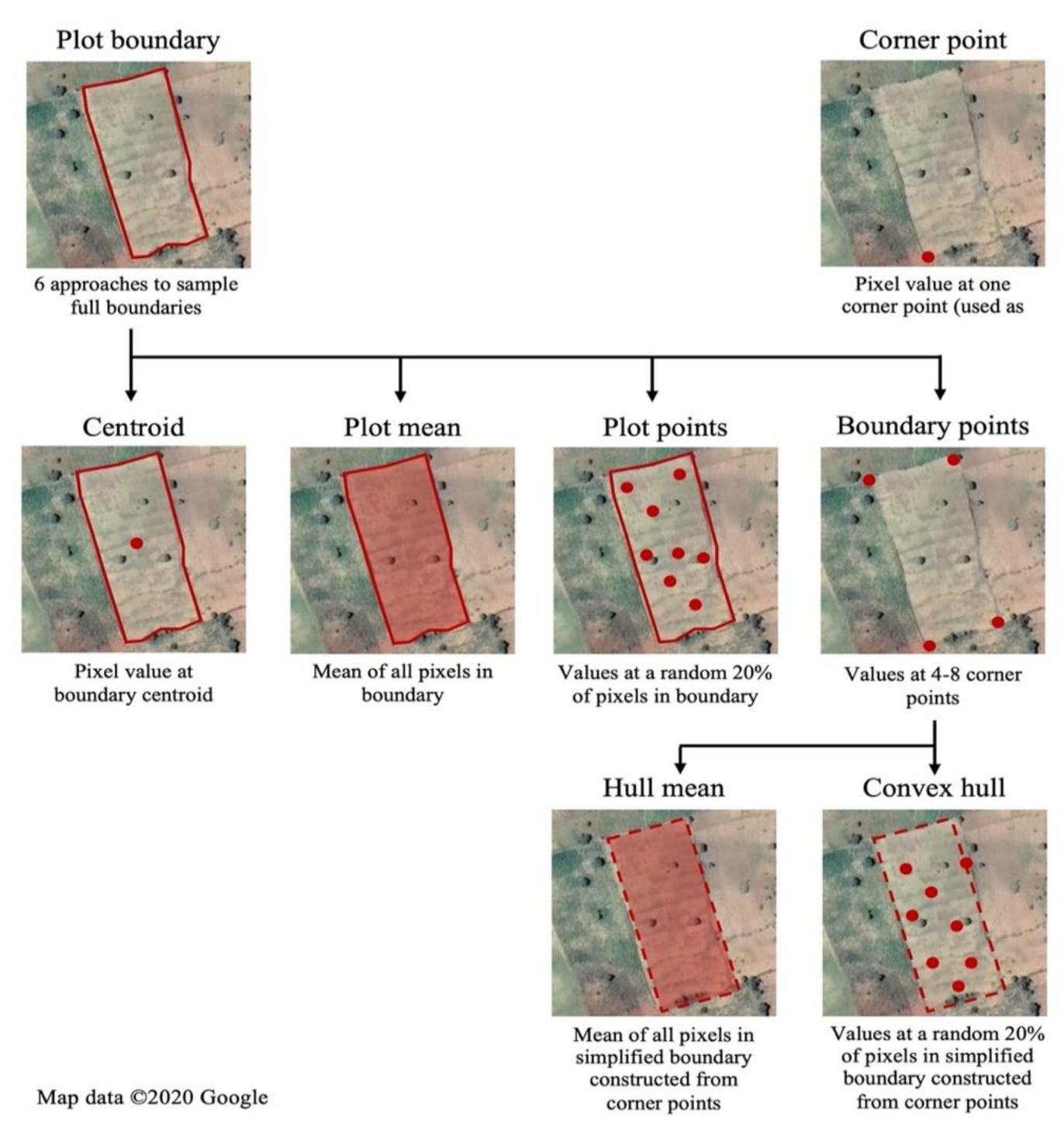
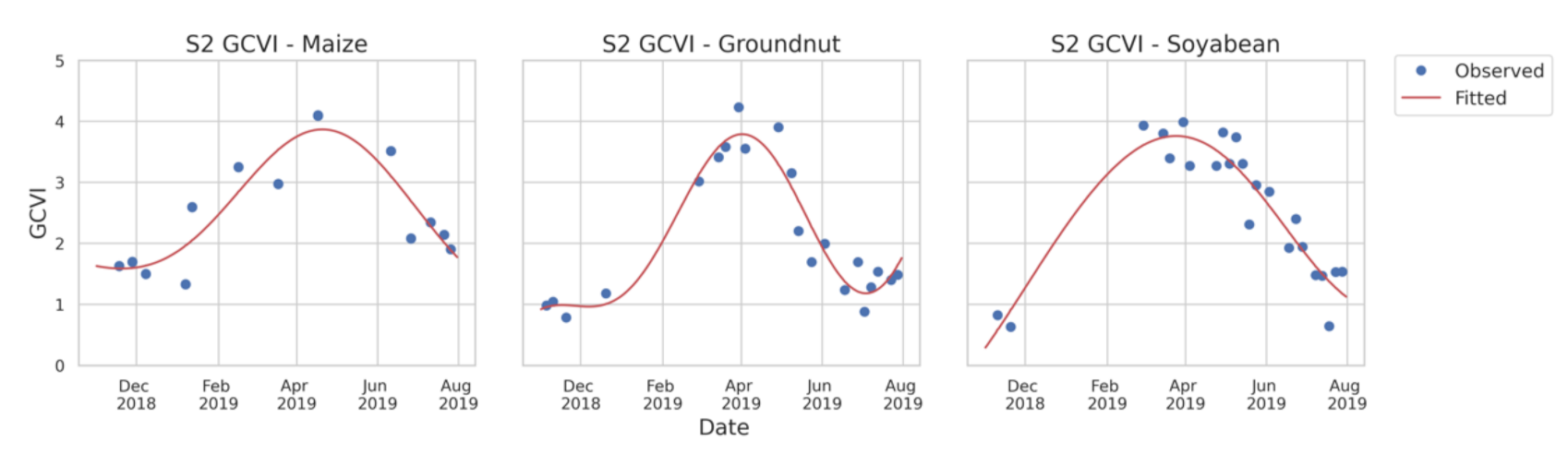
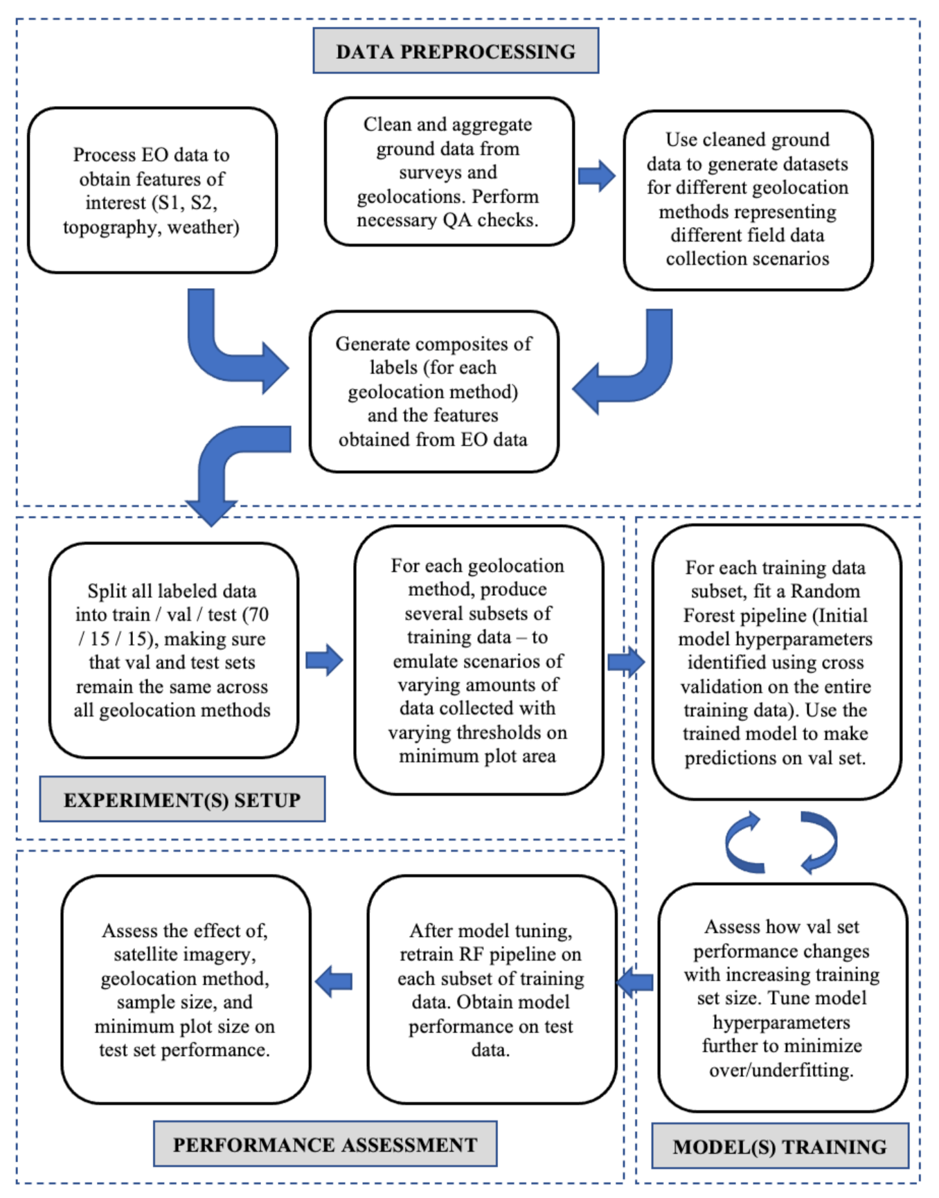
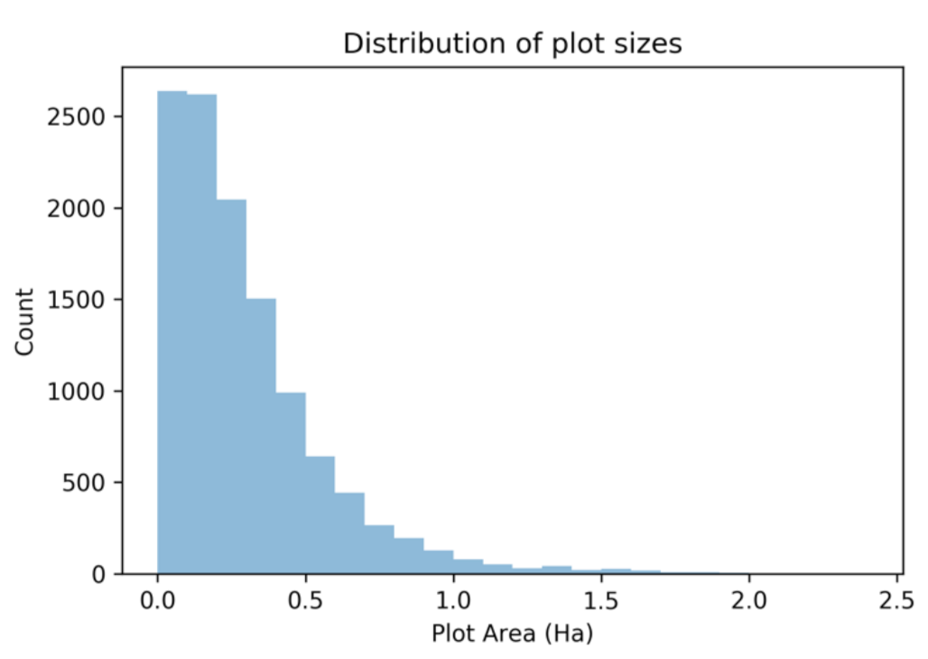
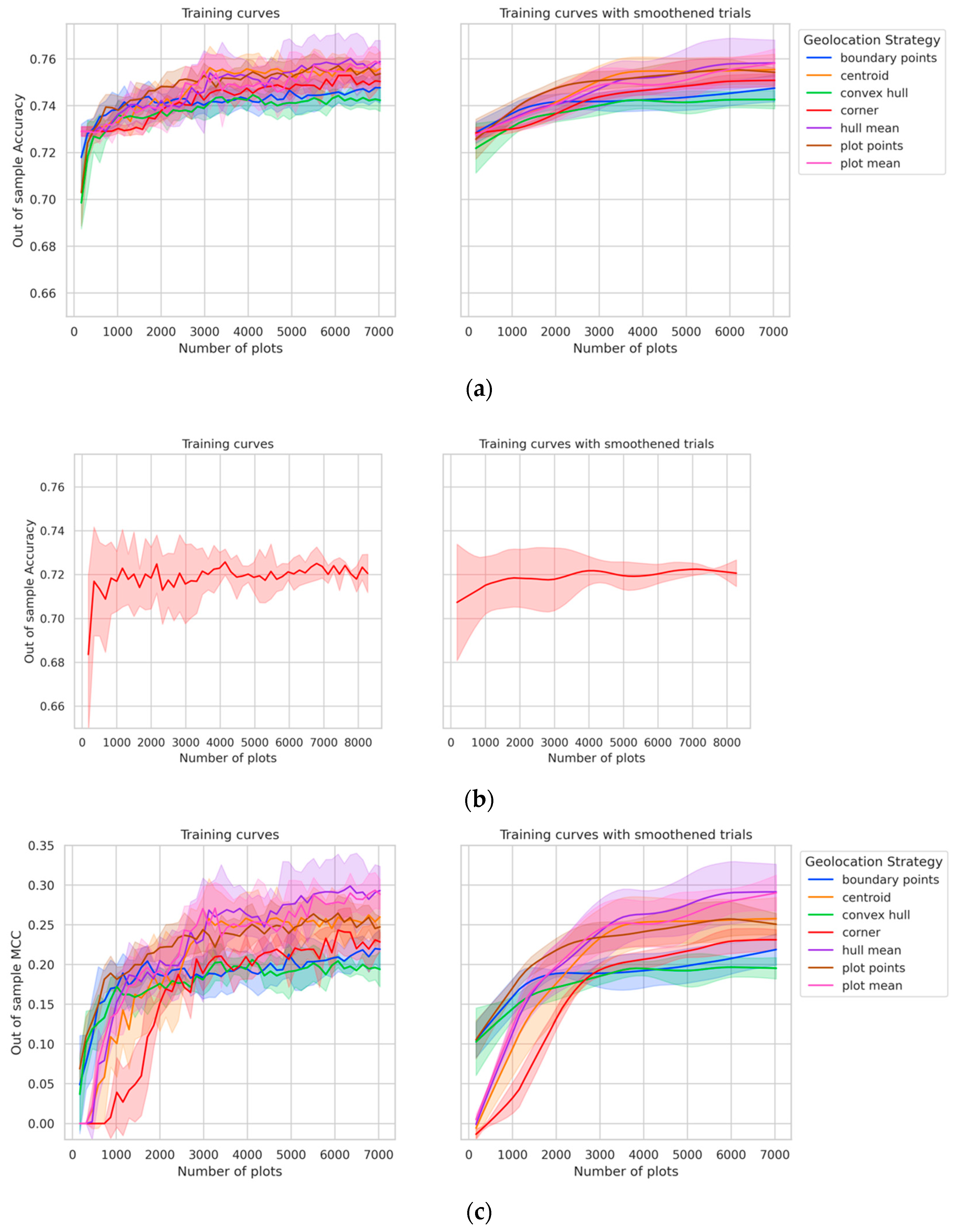
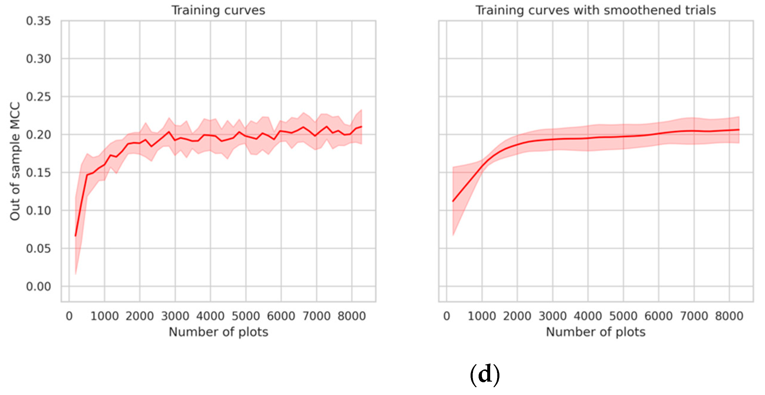
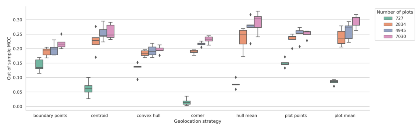
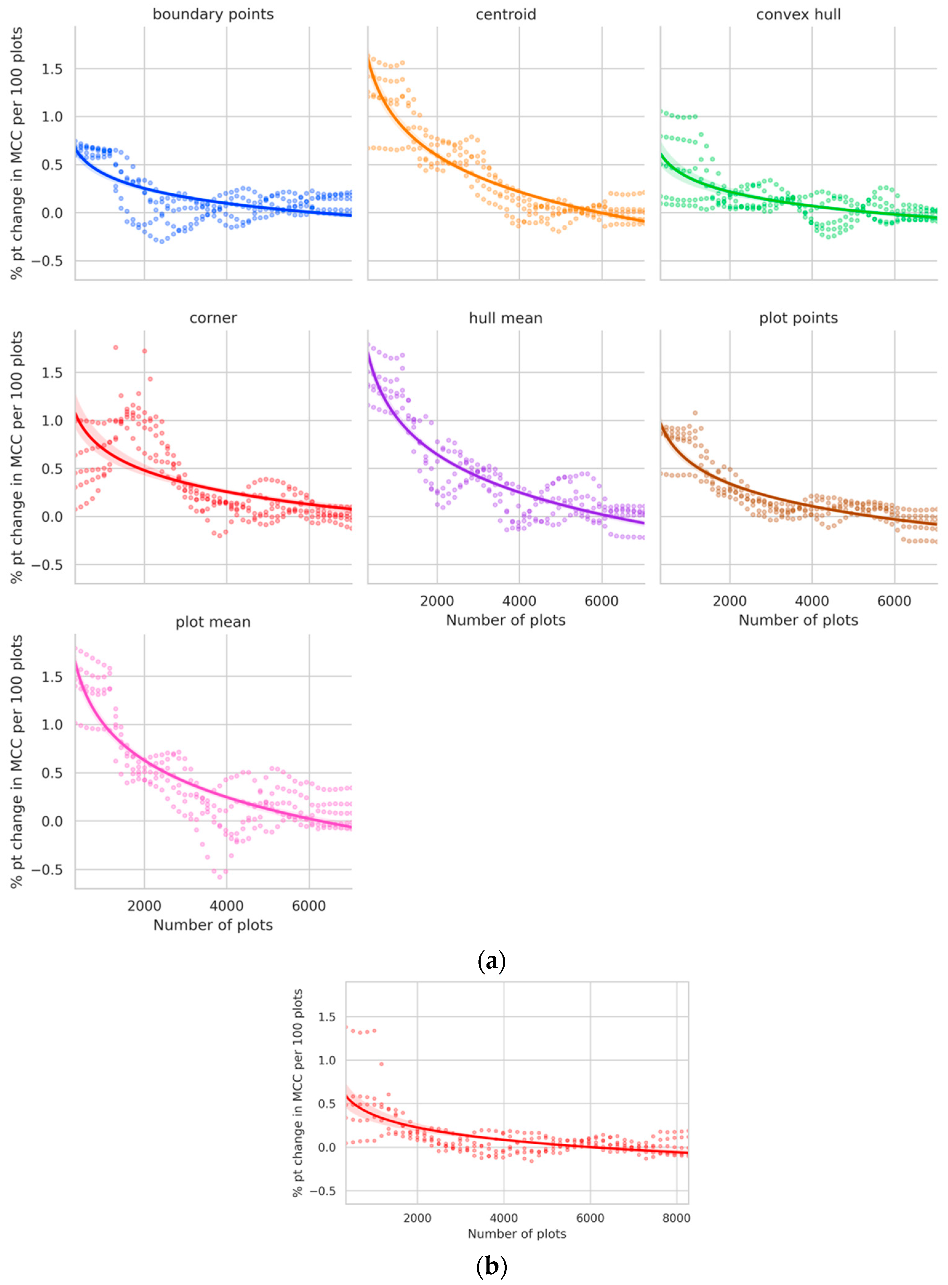
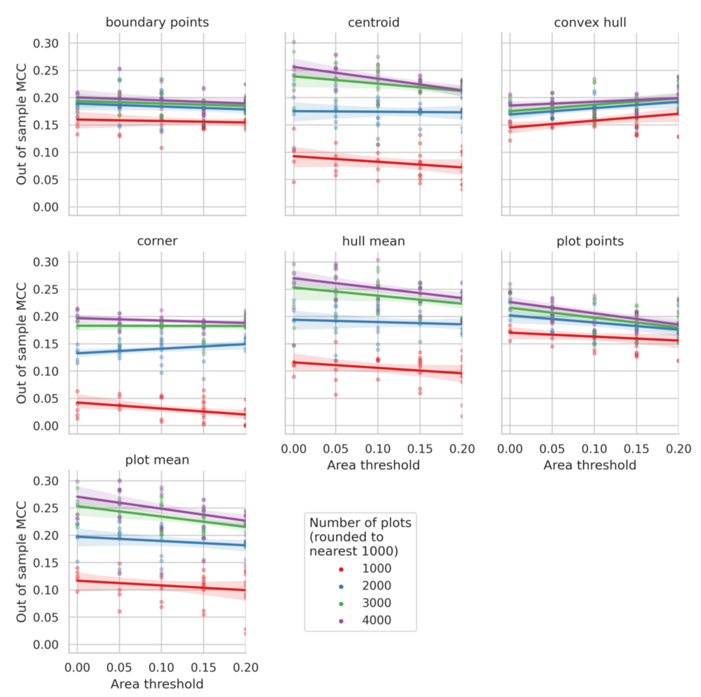
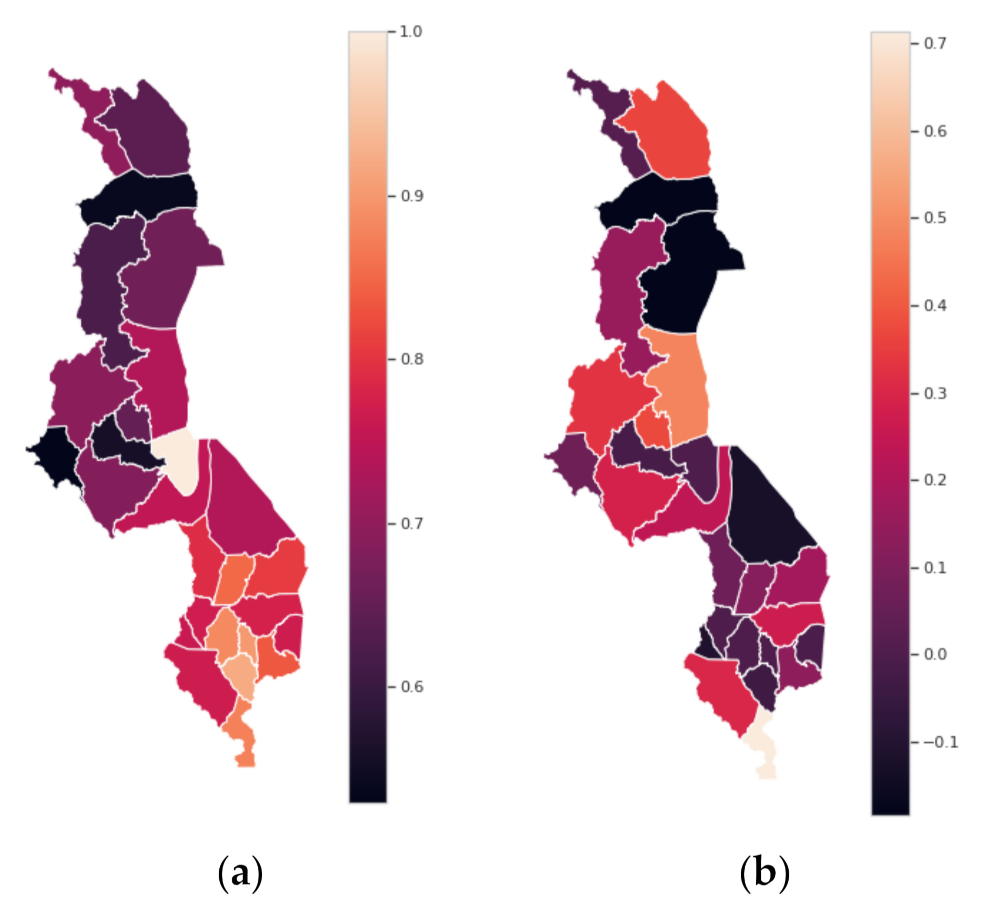
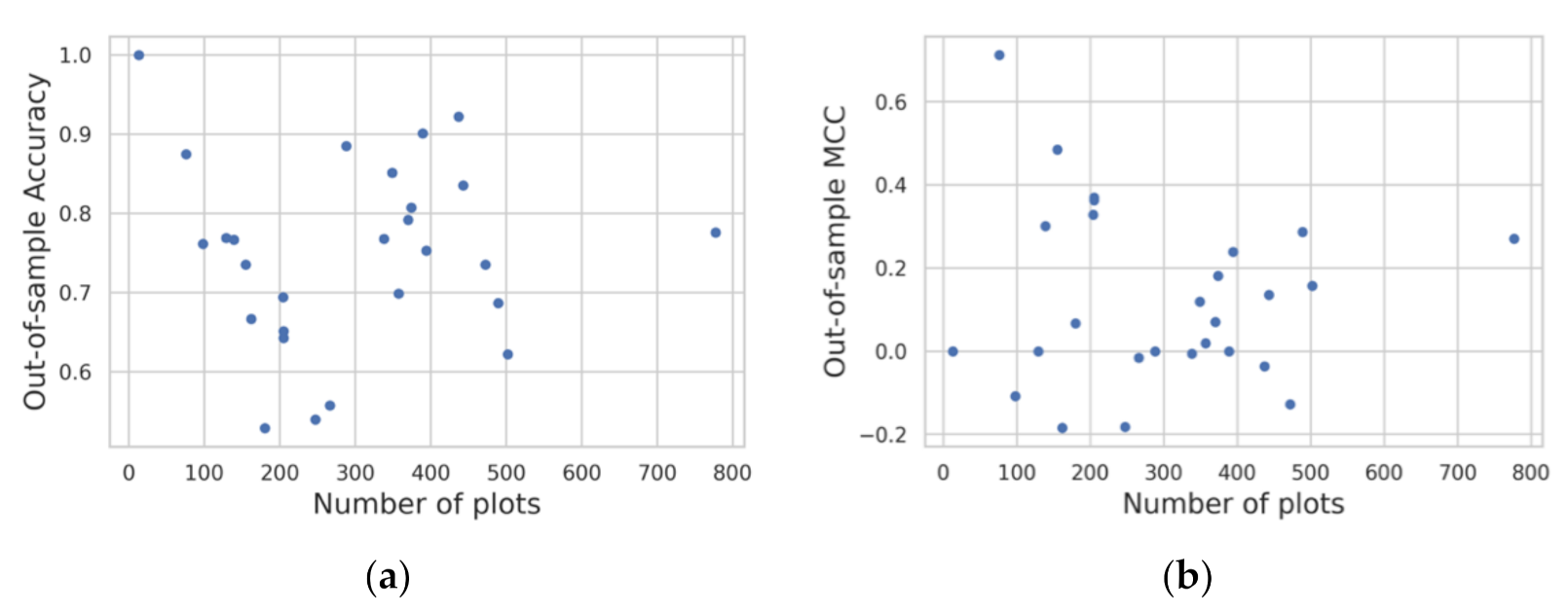
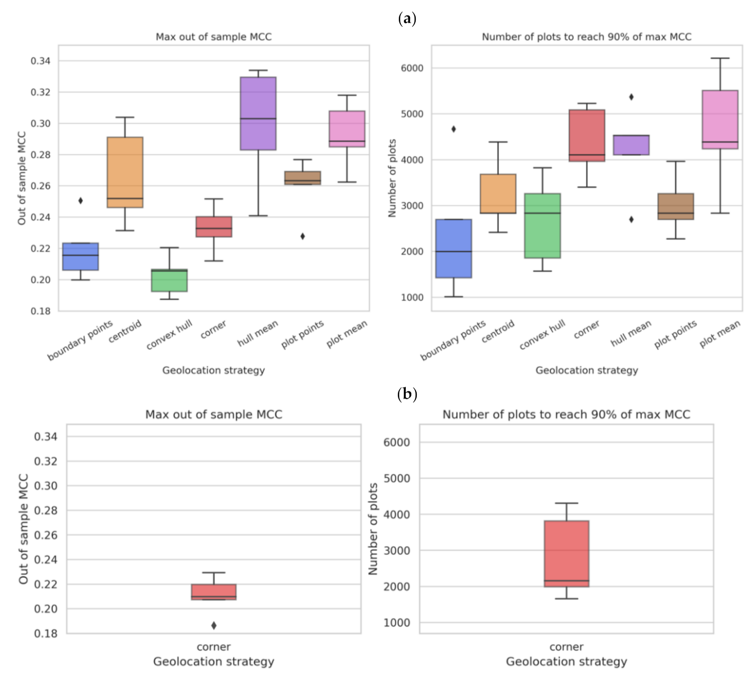


