A Supplementary Module to Improve Accuracy of the Quality Assessment Band in Landsat Cloud Images

Abstract

Cloud contamination is a serious obstacle for the application of Landsat data. To popularize the applications of Landsat data, each Landsat image includes the corresponding Quality Assessment (QA) band, in which cloud and cloud shadow pixels have been flagged. However, previous studies suggested that Landsat QA band still needs to be modified to fulfill the requirement of Landsat data applications. In this study, we developed a Supplementary Module to improve the original QA band (called QA_SM). On one hand, QA_SM extracts spectral and geometrical features in the target Landsat cloud image from the original QA band. On the other, QA_SM incorporates the temporal change characteristics of clouds and cloud shadows between the target and reference images. We tested the new method at four local sites with different land covers and the Landsat-8 cloud cover validation dataset (“L8_Biome”). The experimental results show that QA_SM performs better than the original QA band and the multi-temporal method ATSA (Automatic Time-Series Analyses). QA_SM decreases omission errors of clouds and shadows in the original QA band effectively but meanwhile does not increase commission errors. Besides, the better performance of QA_SM is less affected by the selections of reference images because QA_SM considers the temporal change of land surface reflectance that is not caused by cloud contamination. By further designing a quantitative assessment experiment, we found that the QA band generated by QA_SM improves cloud-removal performance on Landsat cloud images, suggesting the benefits of the new method to advance the applications of Landsat data.

1. Introduction

Landsats provide the longest freely available time-series images with a medium spatial resolution, which have been widely used in many applications (e.g., land cover mapping, [1]). However, a serious obstacle for the applications of Landsat images is frequent cloud contamination because approximately one-third area of the earth is covered by clouds at any given time [2,3]. To use Landsat images more effectively, it is very important to identify clouds and cloud shadows in Landsat cloud images [4].

A number of methods have been proposed to automatically detect clouds and cloud shadows in optical satellite images, which can be roughly divided into two categories. The first category is the single-image methods, which use the multispectral features in the individual cloud image by assuming that clouds are generally brighter than other land cover types at given bands whereas cloud shadows are darker [5,6,7,8,9,10,11]. Moreover, some methods further include more other features, such as the lower temperature of clouds estimated from the thermal infrared bands and the geometric relationship between clouds and cloud shadows. Instead of using these well-defined cloud features, some recent studies employ machine-learning algorithms (e.g., deep learning models) to automatically extract cloud and cloud shadow features [12,13,14,15]. The second category is the multi-temporal methods, which employ the temporal information provided by the images acquired at other times (called “reference images”) [16,17,18,19,20,21]. For example, several multi-temporal methods use the time series of cloud-free Landsat data, such as the multiTemporal mask (Tmask) [21] and the Automatic Time-Series Analyses (ATSA) [21]. They first fit the time series and then compare model estimations with original data in the time series to determine whether these data are cloud-contaminated. There are pros and cons between the single-image methods and the multi-temporal methods. Although the temporal information provides an additional complement to the spectral features for cloud detection, its usefulness depends on the quality of reference images, e.g., the radiometric consistency between the cloud image and reference images [22].

Currently, each Landsat reflectance image has included a Quality Assessment (QA) band, in which cloud and cloud shadow pixels have been flagged. The U.S Geological Survey (USGS) generated the QA band for Landsats 4–8 by using the Function of mask (Fmask) algorithm (version 3.3) [10,11]. Fmask is a single-image method and is recognized to be the most accurate cloud and cloud shadow detection algorithm among single-image methods by testing a number of Landsat cloud images [23]. The objective to produce the QA band is to popularize the application of Landsat data. Naturally, we may wonder whether the Landsat QA band can fulfill the requirement of practical applications? A direct application of the QA band is to reconstruct those cloud-contaminated pixels in the Landsat cloud image [24,25]. Unfortunately, previous studies suggested that the Landsat QA band still needs to be modified to fulfill the requirement of cloud-removal operations [26]. For example, to reduce the influence of cloud omission error in the Landsat QA band on the cloud-removal performance, Zhang et al. [26] conducted a dilation of two pixels around cloud and cloud shadow edges in the Landsat QA band. This simple operation can reduce the omission error to a certain extent because thin clouds are sometimes around thick clouds but is likely to be omitted in the QA band [18]. However, it cannot identify those cloud and cloud shadow patches that are entirely omitted in the QA band. Moreover, it can be expected that the dilation operation may greatly increase commission error in some cases, which is unacceptable particularly for the cloud images with limited cloud-free pixels [10].

In this study, we proposed a simple method to modify the QA band to popularize its application. Since multiple features in the individual Landsat cloud image have been carefully considered in the Fmask algorithm, we assume that the original QA band may be further improved if the new method employs additional temporal features and meanwhile incorporates the information provided by the original QA band. Therefore, our method is based on the original QA band and can be considered as a Supplementary Module to the original QA band (called QA_SM). The use of the original QA band can greatly reduce the complexity to generate cloud and cloud shadow masks. We compared QA_SM with the QA band generated by two other methods, including the original QA band (called QA_original) and the QA band generated by ATSA. ATSA is a state-of-the-art multi-temporal method and was reported to perform better than Fmask particularly for the frequently cloudy areas [20]. An improved QA band is assumed to benefit its practical applications. Taking cloud removal on Landsat cloud images for example, we further quantitatively evaluated the performance of cloud removal with the use of the three different QA bands. The rest of this paper is arranged as follows: The details of QA_SM are described in Section 2. Section 3 provides the experimental designs regarding both cloud detection and the application of cloud removal. The experimental results are given in Section 4 and discussions on the strengths and limitations of the new method are summarized in Section 5.

2. The QA_SM Method

The objective of QA_SM is to improve the original QA band. To acquire additional temporal features, QA_SM employs one reference image that is cloud-free or is with small cloud coverages. To avoid an additional burden of data collections, QA_SM does not require the thermal infrared band and the cirrus band because these bands are either unavailable in Landsat 5 or are usually not collected when using the Landsat optical images.

QA_SM is performed on the Landsat surface reflectance cloud images. To illustrate the method, we used the symbols ${ \mathrm{P}}_{\mathrm{C}}$ and ${ \mathrm{P}}_{\mathrm{CS}}$ to indicate the pixels that were flagged as cloud pixels and cloud shadow pixels in the original QA band of the cloud image, respectively. The other pixels were denoted as the symbol ${ \mathrm{P}}_{\mathrm{other}}$. There are mainly four steps in QA_SM.

2.1. Step1: Identifying the Initial Cloud Pixels

Compared with other ground objects, clouds generally have higher reflectance values in the short wavelengths (e.g., the blue band). Cloud pixels thus have large reflectance changes at the blue band between the cloud image and the reference images. This feature is described by:

$${\mathsf{\rho }}_{\mathrm{blue}}\left(\mathrm{change}\right)=\max \left({\mathsf{\rho }}_{\mathrm{blue}}{\left(\mathrm{cloud}\right) - \mathsf{\rho }}_{\mathrm{blue}}{(\mathrm{ref}}^{’})\right)- \left({\mathsf{\rho }}_{\mathrm{blue}}{\left(\mathrm{cloud}\right) - \mathsf{\rho }}_{\mathrm{blue}}{(\mathrm{ref}}^{’})\right)$$

(1)

where

$${\mathsf{\rho }}_{\mathrm{blue}}\left({\mathrm{ref}}^{’}\right){=\mathsf{\rho }}_{\mathrm{blue}}\left(\mathrm{ref}\right)+\frac{1}{\mathrm{n}}{\displaystyle \sum }_{\mathrm{i}=1}^{\mathrm{n}}{(\mathsf{\rho }}_{\mathrm{blue}}^{\mathrm{i}}\left(\mathrm{cloud}\right){ - \mathsf{\rho }}_{\mathrm{blue}}^{\mathrm{i}}\left(\mathrm{ref}\right)), \mathrm{i}\in {\mathrm{P}}_{\mathrm{other}}^{\mathrm{A}}$$

(2)

${\mathsf{\rho }}_{\mathrm{blue}}^{\mathrm{i}}\left(\mathrm{cloud}\right)$ and ${\mathsf{\rho }}_{\mathrm{blue}}^{\mathrm{i}}\left(\mathrm{ref}\right)$ are the reflectance values at the blue band for a pixel i in the cloud image and the reference image, respectively.${ \mathrm{P}}_{\mathrm{other}}^{\mathrm{A}}$ denotes the class A in ${ \mathrm{P}}_{\mathrm{other}}$, which was generated by using the k-means cluster. The number of classes was set to be 4–5 depending on the Land surface. Here, we employed Equation (2) to reduce the reflectance difference between the cloud and reference images caused by land surface changes. The item $\max \left({\mathsf{\rho }}_{\mathrm{blue}}{\left(\mathrm{cloud}\right)-\mathsf{\rho }}_{\mathrm{blue}}{(\mathrm{ref}}^{’})\right)$ in Equation (1) represents the maximum value of reflectance changes among the pixels in ${ \mathrm{P}}_{\mathrm{other}}$. Those cloud pixels in${ \mathrm{P}}_{\mathrm{C}}$ with the reflectance changes larger than this item are assumed to be the cloud pixels in the final cloud mask (referred to as ${\mathrm{P}}_{\mathrm{C}}^1$), and the other pixels in ${ \mathrm{P}}_{\mathrm{C}}$ are referred to ${\mathrm{P}}_{\mathrm{C}}^2$. Moreover, this item is introduced to make the reflectance change value (${\mathsf{\rho }}_{\mathrm{blue}}\left(\mathrm{change}\right)$) larger than 0; meanwhile, cloud pixels have smaller ${\mathsf{\rho }}_{\mathrm{blue}}\left(\mathrm{change}\right)$.

Another feature of cloud pixels is the relatively large reflectance at the blue band in the cloud image. By combing both large values of ${\mathsf{\rho }}_{\mathrm{blue}}\left(\mathrm{cloud}\right)$ and small values of ${\mathsf{\rho }}_{\mathrm{blue}}\left(\mathrm{change}\right)$ for cloud pixels, a cloud index ($\mathrm{CI}$) is proposed as

$$\mathrm{CI}=\frac{{\mathsf{\rho }}_{\mathrm{blue}}{\left(\mathrm{cloud}\right) - \mathsf{\rho }}_{\mathrm{blue}}\left(\mathrm{change}\right)}{{\mathsf{\rho }}_{\mathrm{blue}}{\left(\mathrm{cloud}\right)+\mathsf{\rho }}_{\mathrm{blue}}\left(\mathrm{change}\right)}+1$$

(3)

with the normalized form, $\mathrm{CI}$ has a value between 0 and 2 and is larger for cloud pixels. We identified initial cloud pixels in ${ \mathrm{P}}_{\mathrm{other}}$ based on the following two criteria: (1) the $\mathrm{CI}$ value of an initial cloud pixel i (denoted as $\mathrm{CI}\left({\mathrm{P}}_{\mathrm{other}}^{\mathrm{i}}\right)$) should be larger than the median $\mathrm{CI}$ value of ${\mathrm{P}}_{\mathrm{C}}^2$, which can be considered to be an absolute threshold condition; (2) we further employed the relative threshold to determine the initial cloud pixels in each class separately. Taking one class as an example, the $\mathrm{CI}$ value of an initial cloud pixel i in the class A (denoted as $\mathrm{CI}\left({\mathrm{P}}_{\mathrm{other}}^{\mathrm{i}}\in \mathrm{A}\right)$) must satisfy the following condition, expressed as:

$$\mathrm{CI}\left({\mathrm{P}}_{\mathrm{other}}^{\mathrm{i}}\in \mathrm{A}\right) > \mathrm{mean}\left(\mathrm{CI}\left({\mathrm{P}}_{\mathrm{other}}^{\mathrm{A}}\right)\right)+\mathrm{a} \times \mathrm{std}\left(\mathrm{CI}\left({\mathrm{P}}_{\mathrm{other}}^{\mathrm{A}}\right)\right)$$

(4)

where $\mathrm{mean}(·)$ is the function of the mean value and $\mathrm{std}(·)$ is the function of the standard deviation. The parameter a is the standard deviation multiplier. A smaller a would lead to more initial cloud pixels, but meanwhile increase the risk of commission errors. We used a value of 2.0 for this parameter (see Section 5).

2.2. Step 2: Identifying the Initial Cloud Shadow Pixels

We proposed a cloud shadow index ($\mathrm{CSI}$) to identify initial cloud shadow pixels. The core idea to construct $\mathrm{CSI}$ is similar to that for $\mathrm{CI}$. $\mathrm{CSI}$ considers the low reflectance values at the near-infrared band (NIR) for cloud shadow pixels in the cloud image (i.e., ${\mathsf{\rho }}_{\mathrm{nir}}\left(\mathrm{cloud}\right)$). And meanwhile, $\mathrm{CSI}$ characterizes the decrease in NIR reflectance for cloud shadow pixels between the reference and cloud images. $\mathrm{CSI}$ was expressed as:

$$\mathrm{CSI}=\frac{{\mathsf{\rho }}_{\mathrm{nir}}{\left(\mathrm{cloud}\right) - \mathsf{\rho }}_{\mathrm{nir}}\left(\mathrm{change}\right)}{{\mathsf{\rho }}_{\mathrm{nir}}{\left(\mathrm{cloud}\right)+\mathsf{\rho }}_{\mathrm{nir}}\left(\mathrm{change}\right)}+1$$

(5)

where

$${\mathsf{\rho }}_{\mathrm{nir}}\left(\mathrm{change}\right)=\left({\mathsf{\rho }}_{\mathrm{nir}}{(\mathrm{ref}}^{’}{) - \mathsf{\rho }}_{\mathrm{nir}}\left(\mathrm{cloud}\right)\right) - \min \left({\mathsf{\rho }}_{\mathrm{nir}}{(\mathrm{ref}}^{’}{) - \mathsf{\rho }}_{\mathrm{nir}}\left(\mathrm{cloud}\right)\right)$$

(6)

$${\mathsf{\rho }}_{\mathrm{nir}}\left({\mathrm{ref}}^{’}\right){=\mathsf{\rho }}_{\mathrm{nir}}\left(\mathrm{ref}\right)+\frac{1}{\mathrm{n}}{\displaystyle \sum }_{\mathrm{i}=1}^{\mathrm{n}}{(\mathsf{\rho }}_{\mathrm{nir}}^{\mathrm{i}}\left(\mathrm{cloud}\right) {- \mathsf{\rho }}_{\mathrm{nir}}^{\mathrm{i}}\left(\mathrm{ref}\right)), \mathrm{i}\in {\mathrm{P}}_{\mathrm{other}}^{\mathrm{A}}$$

(7)

$\min (·)$ is the function of the minimum value. Those cloud shadow pixels in${ \mathrm{P}}_{\mathrm{C}}$ with the reflectance changes smaller than the item $\min \left({\mathsf{\rho }}_{\mathrm{nir}}{(\mathrm{ref}}^{’}{) - \mathsf{\rho }}_{\mathrm{nir}}\left(\mathrm{cloud}\right)\right)$ are assumed to be the cloud shadow pixels in the final cloud shadow mask (referred to as ${\mathrm{P}}_{\mathrm{CS}}^1$), and the other pixels in ${ \mathrm{P}}_{\mathrm{CS}}$ are referred to ${\mathrm{P}}_{\mathrm{CS}}^2$. $\mathrm{CSI}$ has a value between 0 and 2, and is smaller for cloud shadow pixels. A pixel i in ${ \mathrm{P}}_{\mathrm{other}}$ (denoted as $\mathrm{CSI}\left({\mathrm{P}}_{\mathrm{other}}^{\mathrm{i}}\right)$) was identified to be an initial cloud shadow pixel if the following two criteria were satisfied: (1) $\mathrm{CI}\left({\mathrm{P}}_{\mathrm{other}}^{\mathrm{i}}\right)$ should be smaller than the median $\mathrm{CSI}$ value of ${\mathrm{P}}_{\mathrm{CS}}^2$, which can be considered to be an absolute threshold; (2) a relative threshold was employed to determine initial cloud shadow pixels in each class separately. For example, the $\mathrm{CSI}$ value of an initial cloud shadow pixel i in class A (denoted as $\mathrm{CSI}\left({\mathrm{P}}_{\mathrm{other}}^{\mathrm{i}}\in \mathsf{A}\right)$) should follow the following equation:

$$\mathrm{CSI}\left({\mathrm{P}}_{\mathrm{other}}^{\mathrm{i}}\in \mathsf{A}\right) < \mathrm{mean}\left(\mathrm{CSI}\left({\mathrm{P}}_{\mathrm{other}}^{\mathrm{A}}\right)\right)-\mathrm{b} \times \mathrm{std}\left(\mathrm{CSI}\left({\mathrm{P}}_{\mathrm{other}}^{\mathrm{A}}\right)\right)$$

(8)

where the parameter $\mathrm{b}$ is the standard deviation multiplier and was set to be 2.0 (see Section 5).

2.3. Step 3: Matching the Initial Cloud and Cloud Shadow Pixels

Clouds always accompany cloud shadows. Therefore, we refined the initial cloud and cloud shadow pixels by using the relationship of geometric locations among clouds, cloud shadows, and the sun. Assuming an initial cloud pixel i is located at $(\mathrm{x},\mathrm{y})$, the corresponding cloud shadow pixel can be found at (x′,y′) according to the following equations [27]

$${\mathrm{x}’=\mathrm{x} - \mathrm{H}}_{\mathrm{cloud}\text{\_}\mathrm{i}} \times \tan \mathsf{\theta }\times \sin \mathsf{\varphi }$$

(9)

$${\mathrm{y}’}^{ }{=\mathrm{y}+\mathrm{H}}_{\mathrm{cloud}\text{\_}\mathrm{i}} \times \tan \mathsf{\theta }\times \cos \mathsf{\varphi }$$

(10)

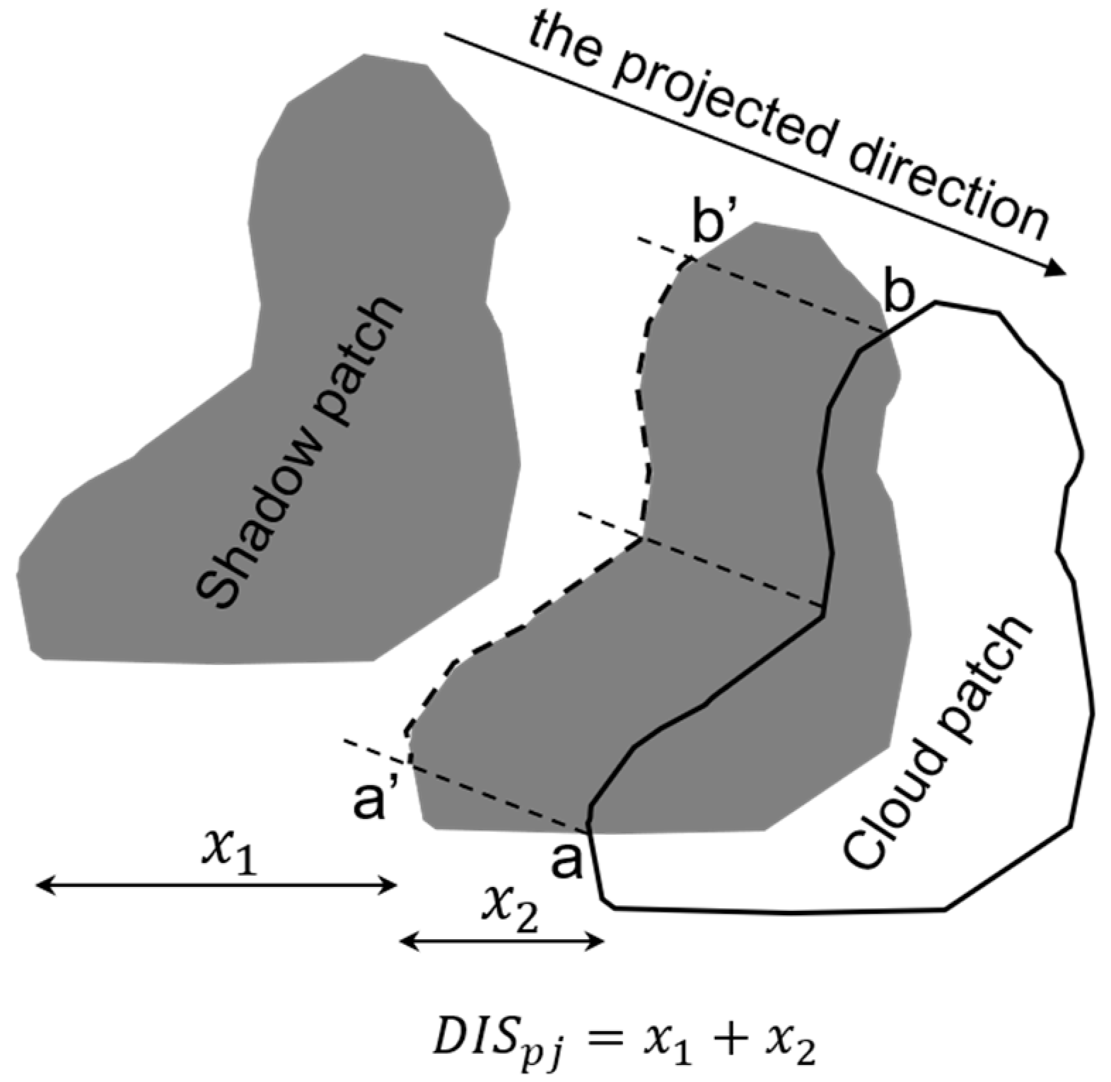
where $\mathsf{\theta }$ is the solar zenith angle and $\mathsf{\varphi }$ is the solar azimuth angle, both of which are provided by the image metadata file. ${\mathrm{H}}_{\mathrm{cloud}\text{\_}\mathrm{i}}$ is the cloud height at the location ($\mathrm{x},\mathrm{y}$). Some previous methods estimated the height of each cloud patch based on lapse rates for air temperature from land surface to clouds [6,10]. However, QA_SM did not employ the thermal infrared band to estimate ${\mathrm{H}}_{\mathrm{cloud}\_\mathrm{i}}$. Those clouds that were omitted in the QA band are normally thin. The brightness temperature of thin clouds is greatly affected by the land surface. As a solution, QA_SM estimated a possible range of ${\mathrm{H}}_{\mathrm{cloud}\text{\_}\mathrm{i}}$ based on the original QA band. We assumed that ${\mathrm{H}}_{\mathrm{cloud}\text{\_}\mathrm{i}}$ is within the range of cloud heights for those cloud pixels that were flagged in the QA band. For this, we generated the cloud patches and cloud shadow patches in the QA band according to the eight-neighborhood connectedness. For a cloud patch j, its height (${\mathrm{H}}_{\mathrm{cloud}\text{\_}\mathrm{pj}}$) can be estimated approximately from the horizontal distance between this cloud patch and its shadow patch (denoted as ${\mathrm{DIS}}_{\mathrm{pj}}$), given by

$${\mathrm{H}}_{\mathrm{cloud}\text{\_}\mathrm{pj} }=\frac{{\mathrm{DIS}}_{\mathrm{pj}}}{\sqrt{{(\tan \mathsf{\theta }\times \sin \mathsf{\varphi })}^2+(\tan \mathsf{\theta }\times \cos \mathsf{\varphi }{)}^2}}$$

(11)

We estimated ${\mathrm{DIS}}_{\mathrm{pj}}$ automatically by two steps (Figure 1). First, the shadow patch was moved along the projected direction until the overlap area between the cloud and shadow patches reaches one-third of the area of the shadow patch. The horizontal distance of movement is assumed to be ${\mathrm{x}}_1$. The boundary of the cloud patch intercepted by the shadow patch is denoted as the curve $\mathrm{ab}$. In the second step, the curve $\mathrm{ab}$ was matched with the corresponding boundary of the shadow patch (i.e., a′b′) based on the similar shapes of the two curves. We enabled the two curves to have an identical length by linear interpolation and calculated the correlation coefficient between them. We assumed a successful match if the correlation coefficient is above 0.9. The horizontal distance between the two curves is denoted as ${\mathrm{x}}_2$. Thus, ${\mathrm{DIS}}_{\mathrm{pj}}$ is the sum of ${\mathrm{x}}_1$ and ${\mathrm{x}}_2$ (Figure 1). For some clouds such as the ones with large vertical extents, their heights may not be estimated if the shapes of the two curves are less similar (i.e., correlation coefficient < 0.9). Assuming that we estimated the heights of n cloud patches in the QA band (i.e., ${\text{{}\mathrm{H}}_{\mathrm{cloud}\text{\_}\mathrm{p}1},\dots {,\mathrm{H}}_{\mathrm{cloud}\text{\_}\mathrm{pn}}\text{}}$), the possible range of ${\mathrm{H}}_{\mathrm{cloud}\text{\_}\mathrm{i}}$ is thus estimated to be

$${\min \text{{}\mathrm{H}}_{\mathrm{cloud}\text{\_}\mathrm{p}1}{,\dots ,\mathrm{H}}_{\mathrm{cloud}\text{\_}\mathrm{pn}}\text{}} \le { \mathrm{H}}_{\mathrm{cloud}\text{\_}\mathrm{i}} \le { \max \text{{}\mathrm{H}}_{\mathrm{cloud}\text{\_}\mathrm{p}1}{,\dots ,\mathrm{H}}_{\mathrm{cloud}\text{\_}\mathrm{pn}}\text{}}$$

(12)

We removed the maximum 1% values from ${\text{{}\mathrm{H}}_{\mathrm{cloud}\text{\_}\mathrm{p}1},\dots {,\mathrm{H}}_{\mathrm{cloud}\text{\_}\mathrm{pn}}\text{}}$ to make the estimation of ${\mathrm{H}}_{\mathrm{cloud}\text{\_}\mathrm{i}}$ less affected by outliers. QA_SM allowed the heights of the initial cloud pixels can vary in the possible range, and thereby matched all initial cloud and cloud shadow pixels by using different heights.

An initial cloud shadow pixel was preserved once its corresponding cloud pixel can be found. For an initial cloud pixel, its projected pixel may be also covered by clouds (e.g., large clouds). If so, QA_SM started with this projected pixel and determined the next projected pixel. This process was continued until the projected pixel is a cloud shadow pixel or a cloud-free pixel. If it is a cloud shadow pixel, this initial cloud pixel was preserved; otherwise, this initial cloud pixel was removed.

2.4. Step 4: Generating the Final QA Band

In the first three steps, we expected to reduce the omission error by detecting cloud and cloud shadow pixels in ${ \mathrm{P}}_{\mathrm{other}}$. In this step, we aim to reduce the commission error to some extent. We assumed that a cloud pixel in ${ \mathrm{P}}_{\mathrm{C}}$ was flagged as cloud-free if the CI value of this pixel was smaller than the median CI value of cloud-free pixels in ${ \mathrm{P}}_{\mathrm{other}}$. Similar operations were performed for cloud shadow pixels in ${ \mathrm{P}}_{\mathrm{C}}$ by using the CSI values. To further reduce commission error, we followed previous studies (e.g., [20]) to remove isolated cloud-contaminated pixels. Cloud patches and cloud shadow patches in QA_SM were removed if they had much smaller sizes (i.e., <7 pixels by using the eight-neighborhood connectedness).

QA_SM inherited the snow mask and the water mask in the original QA band because of two reasons: first, Fmask is a sophisticated algorithm and identifies snow and water by using multiple features (e.g., multi-band thresholds) and data sources (e.g., global water map) [28]. QA_SM is based on the original QA band and thus does not include snow and water detections, which substantially reduces the complexity of the supplementary module. Second, QA_SM is developed to popularize the Landsat data application. We indeed found that snow and clouds are sometimes confused in the original QA band, but it may be unnecessary to distinguish the two types because both of them were usually excluded from many practical applications such as vegetation studies.

3. Data and Experiments

We conducted two groups of experiments to evaluate QA_SM. In experiment I, we tested QA_SM at four local test sites to answer three questions: first, whether the QA band generated by QA_SM has higher accuracy than those generated by other methods; Second, we took the cloud-removal application as the example to investigate whether the improved QA band by QA_SM can really benefit the application of Landsat cloud images; Third, since QA_SM uses a cloud-free reference image acquired at another time, we investigated whether and to what extent the performance of QA_SM is affected by the different selections of reference images. In the experiment II, we performed more extensive evaluations for cloud detection by applying QA_SM to the Landsat-8 cloud cover validation dataset (“L8_Biome”) [23].

3.1. Experiment I: Evaluations at Four Test Sites of China

3.1.1. Experiment I Design

We collected Landsat 8 Land surface reflectance images at four test sites in China. Because geometrical error for Landsat reflectance data is normally within a pixel, we did not perform additional registration.

Table 1. Upper: the Landsat 8 image information at the four test sites for the experiment of cloud detection (upper); Lower: the cloud-simulated images for the quantitative assessments of cloud removal. SSIM: the Structure SIMilarity index.

	Test Sites (Path/Row)	North China Plain (123/34)	Southeastern China (126/44)	Hang Zhou (119/39)	Tibetan Plateau (138/39)
Cloud detection	Actual cloud image	2017-05-23	2016-10-16	2016-04-22	2019-06-07
	Reference image 1 (SSIM)	2017-05-07 (0.898)	2017-04-10 (0.678)	2015-10-13 (0.779)	2018-02-12 (0.641)
	Reference image 2 (SSIM)	2018-04-08 (0.739)	2014-10-11 (0.656)	2017-05-27 (0.731)	2018-01-27 (0.599)
	Image size	$950\times 950$	$1000\times 1000$	$919\times 921$	$1003\times 1003$
Cloud removal	Cloud-simulated image	2016-05-04	2017-05-28	2014-05-23	2016-11-21

summarized the image information at each site. The first site is double-cropping cropland in the North China Plain where ground reflectance values change rapidly. At this site, summer maize or soybean is normally planted in mid-June after harvesting the winter wheat [29]. The second site is an evergreen forest area in Southeastern China, which belongs to a subtropical monsoon climate with frequent cloud contamination. The third site is urban Hangzhou, China. This urban site is experiencing rapid urbanization and has a heterogeneous landscape. The fourth site locates in the Tibetan Plateau with snow cover and complex terrain.

Firstly, we performed both the visual assessments and quantitative evaluations for the cloud masks generated by different methods (i.e., QA_original, QA_SM, and ATSA) at the four test sites. Three evaluation indices were adopted, including the Commission error, Omission error, and F1-score of the mask, expressed as:

$$\mathrm{Commission}=1 - \frac{\mathrm{agreement} \mathrm{of} \mathrm{clouds} \mathrm{and} \mathrm{shadows} }{\mathrm{agreement} \mathrm{of} \mathrm{clouds} \mathrm{and} \mathrm{shadows}+\mathrm{commission} \mathrm{of} \mathrm{clouds} \mathrm{and} \mathrm{shadows}}$$

(13)

$$\mathrm{Omission}=1 - \frac{\mathrm{agreement} \mathrm{of} \mathrm{clouds} \mathrm{and} \mathrm{shadows}}{\mathrm{agreement} \mathrm{of} \mathrm{clouds} \mathrm{and} \mathrm{shadows}+\mathrm{omission} \mathrm{of} \mathrm{clouds} \mathrm{and} \mathrm{shadows}}$$

(14)

$$\mathrm{F}1=\frac{2 \times \mathrm{agreement} \mathrm{of} \mathrm{clouds} \mathrm{and} \mathrm{shadows}}{2 \times \mathrm{agreement} \mathrm{of} \mathrm{clouds} \mathrm{and} \mathrm{shadows}+\mathrm{omission} \mathrm{of} \mathrm{clouds} \mathrm{and} \mathrm{shadows}+\mathrm{commission} \mathrm{of} \mathrm{clouds} \mathrm{and} \mathrm{shadows}}$$

(15)

The reference cloud masks were visually interpreted carefully by the independent analysts. Considering that a satisfactory reference image may be unavailable in some cases, we tested the performance of QA_SM by using different reference images. These reference images have different similarities to the cloud image. The Structure SIMilarity index (SSIM) [30] was calculated to measure the structural similarity between the cloud-free areas in the cloud image and the corresponding areas in the reference image (Table 1).

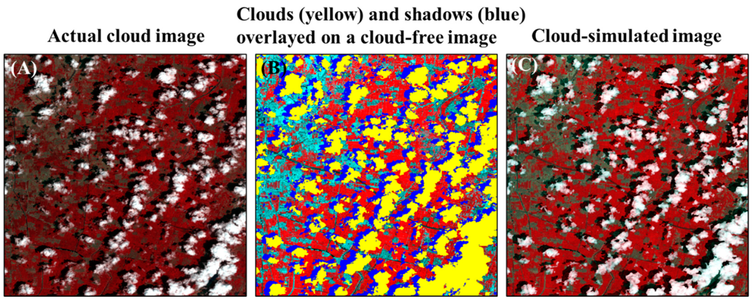
Secondly, we further quantitatively assessed the influence of different QA bands on the cloud-removal performance. This experiment can be considered as an example of the practical application of the QA band. Because the true reflectance values of cloud and cloud shadow pixels are unknown, it is impossible to conduct this experiment on the actual Landsat cloud images. We thus performed this experiment on the cloud-simulated image at each site (see the last row in Table 1). Specifically, the cloud-simulated image was generated based on a cloud-free image in two steps: first, we simulated the cloud and cloud shadow masks on the cloud-simulated image by overlapping the reference mask of an actual cloud image on the cloud-free image (see Figure 2A,B); Second, the reflectance values of clouds and cloud shadows in the cloud-simulated image were simulated by using the atmospheric radiative transfer code MODTRAN (version 5.2.2) [31], which is demonstrated in detail in Section 3.1.2. For cloud removal on the cloud-simulated image, we used the different QA bands of this actual cloud image (i.e., QA_original, QA_SM and QA_ATSA of the actual cloud image). We employed two different cloud-removal methods to reconstruct the cloud and cloud shadow pixels, including the local linear histogram matching (LLHM) method [32] and the modified neighborhood similar pixel interpolator (MNSPI) method [33]. LLHM reconstructs each cloud patch in the target cloud image by using a linear transfer function, which is determined by performing histogram matching for the neighboring pixels around each cloud patch between the target and the reference images. MNSPI combines both spatial-based and temporal-based estimations to fill cloud-induced missing reflectance. Two indices were adopted for quantitative assessments. The first is the root mean square error (RMSE), which measures the difference between the reconstructed reflectance values and the true values. Because the reconstructed pixels are different for various QA bands, RMSE was calculated for the pixels in the union of the three different QA bands (i.e., QA_original ∪ QA_SM ∪ ATSA). The second index is the SSIM values [30], which measure the structural similarity between the reconstructed image and the true image.

3.1.2. The Reflectance Values of Cloud and Cloud Shadow Pixels Simulated by MODTRAN

The reflectance values of cloud and cloud shadow pixels were simulated by MODTRAN (version 5.2.2). MODTRAN is a classic 1D model in which the atmosphere is considered to be plane-parallel and vertically inhomogeneous. By assuming a Lambertian surface, the reflectance at the top of the atmosphere (${\mathsf{\rho }}_{\mathrm{TOA}}$) can be estimated from

$${\mathsf{\rho }}_{\mathrm{TOA}}{=\mathsf{\rho }}_0+\frac{\left({\mathrm{T}}_{\mathrm{s}}{+\mathrm{t}}_{\mathrm{s}}\right)(\mathrm{T}+\mathrm{t})\mathsf{\rho }}{1 - \mathsf{\rho }\mathsf{\sigma }}$$

(16)

where $\mathsf{\rho }$ is the ground reflectance. ${\mathsf{\rho }}_0$ is the path reflectance from the atmosphere. ${\mathrm{T}}_{\mathrm{s}}$ and ${\mathrm{t}}_{\mathrm{s}}$ are the direct and diffuse transmittance from the sun to the ground. T and $\mathrm{t}$ are the direct and diffuse transmittance from ground to sensor. $\mathsf{\sigma }$ is the atmospheric spherical albedo. By solving this equation inversely, we can acquire

$$\mathsf{\rho }=\frac{{\mathsf{\rho }}_{\mathrm{TOA}}-{\mathsf{\rho }}_0}{{(\mathsf{\rho }}_{\mathrm{a}}-{\mathsf{\rho }}_0)\mathsf{\sigma }+\left({\mathrm{T}}_{\mathrm{s} }{+\mathrm{t}}_{\mathrm{s}}\right)(\mathrm{T}+\mathrm{t})}$$

(17)

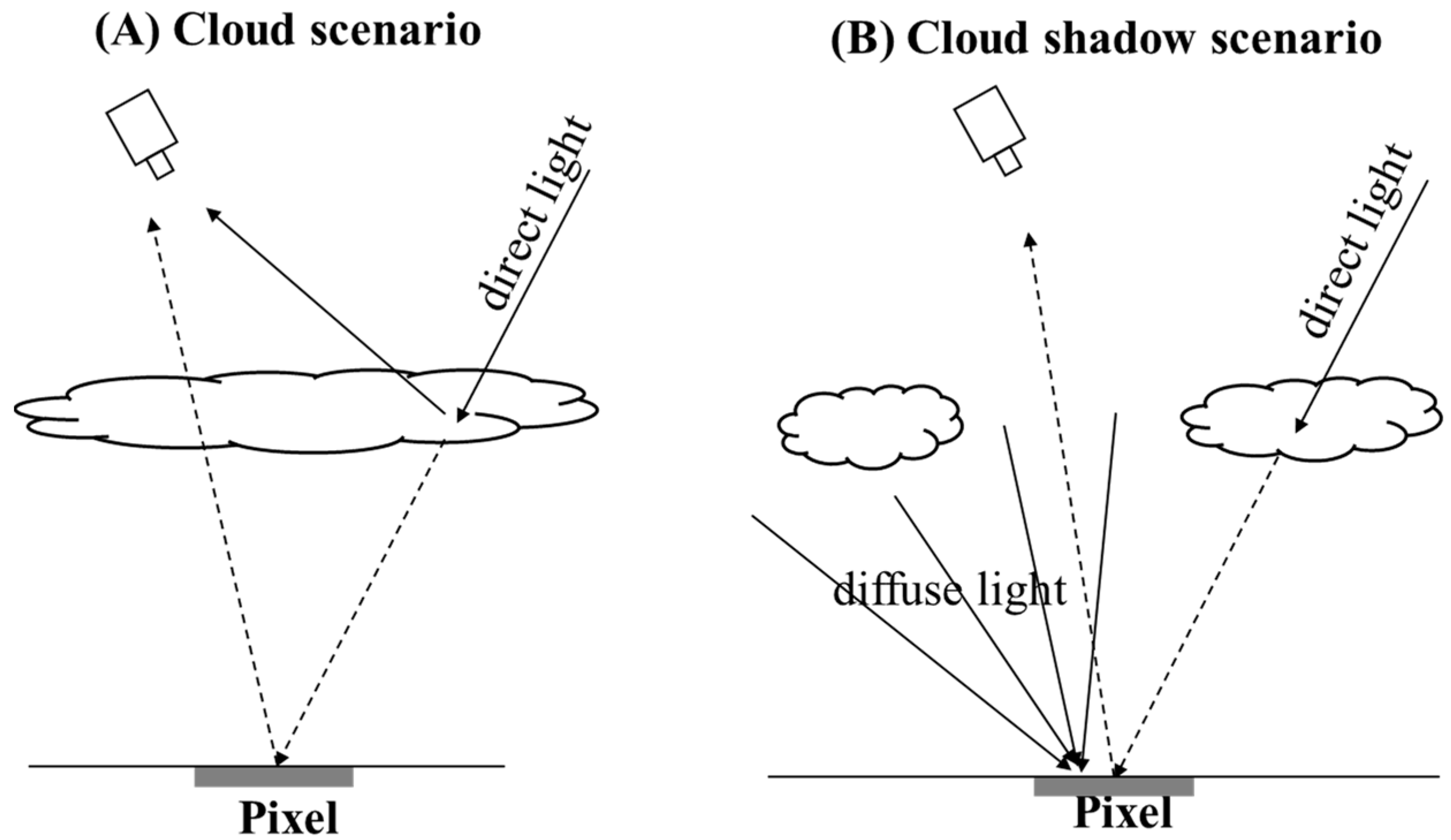
Equations (16) and (17) are the basis of the simulations. For those pixels located in the cloud mask (Figure 3A), we first transformed their ground reflectance to ${\mathsf{\rho }}_{\mathrm{TOA}}$ based on Equation (16). The atmospheric variables in Equation (16) (i.e., ${\mathsf{\rho }}_0$, ${\mathrm{T}}_{\mathrm{s}}$, ${\mathrm{t}}_{\mathrm{s}}$, T, $\mathrm{t}$, and $\mathsf{\sigma }$) were determined by running the cloud model in MODTRAN. We called this process “forward simulation”. Next, we transformed the simulated ${\mathsf{\rho }}_{\mathrm{TOA}}$ to the ground reflectance based on Equation (17), but the atmospheric variables in Equation (17) were generated by running the clear-sky model in MODTRAN. This process was called “backward simulation”, which simulated the operation of atmospheric correction. We considered varying cloud thickness for cloud pixels by using the haze optimal transformation (HOT) as an indicator of cloud thickness [34]. The HOT values were calculated for those cloud pixels in the actual cloud image and were converted to thickness by the simple linear function. The conversion coefficients were tuned on the individual image.

We simulated the reflectance values of cloud shadow pixels by assuming the partly cloudy condition (Figure 3B). Likewise, both forward and backward simulations were adopted. In the forward simulation, the cloud shadow pixel is illuminated by the atmospheric diffuse light and the direct light that is blocked by clouds. Given that the atmospheric diffuse light may also be blocked by clouds to some extent, we incorporated an adjusting factor (named ${\mathrm{V}}_{\mathrm{f}}$) into Equation (16), expressed as

$${\mathsf{\rho }}_{\mathrm{TOA}}{=\mathsf{\rho }}_0+\frac{\left({\mathrm{T}}_{\mathrm{s} }{+\mathrm{V}}_{\mathrm{f}}{\mathrm{t}}_{\mathrm{s}}\right){(\mathrm{T}+\mathrm{V}}_{\mathrm{f}}\mathrm{t})\mathsf{\rho }}{1 - \mathsf{\rho }\mathsf{\sigma }}$$

(18)

${\mathrm{V}}_{\mathrm{f}}$ was employed to account for the effective cloud fraction, thereby having a value between 0–1. ${\mathrm{V}}_{\mathrm{f}}$ was tuned on the individual image to reconcile the brightness of shadows between the actual could image and the cloud-simulated image. For each shadow pixel, the location of the corresponding cloud pixel was determined by the geometrical matching (i.e., Equations (9) and (10)). Figure 2C shows the cloud-simulated image at the site of the North China Plain (for the cloud-simulated images at all sites, please refer to Figure S1 in the Supplementary Materials).

3.2. Experiment II: Tests on the Landsat 8 Cloud Cover Validation Dataset

In this experiment, we performed extensive tests for cloud detection on the Landsat-8 cloud cover validation dataset (“L8_Biome”) [23]. In L8_Biome, there are 32 Landsat 8 scenes with both manual cloud mask and cloud shadow mask. These images are globally distributed and are covered by eight different biomes, i.e., forest, grass/crops, shrubland, barren, urban, snow/ice, water and wetland. We excluded five images belonging to the snow/ice biome because QA_SM inherited the snow/ice mask in the original QA band and ATSA also does not include the snow/ice detection module. Besides, five images with a cloud coverage of less than 1% were excluded because cloud commission error is tolerable in these images. The 22 Landsat scenes employed for this experiment were shown in

Table 2. The image information of the 22 Landsat scenes in experiment II.

L8_Biome Site (Path/Row)	Center Latitude/Longitude	Image Date	Cloud Coverage
Barren_1 (P193/R45)	22°4′ N/2°2′ E	2013-05-06	64.06%
Barren_2 (P 164/R60)	15°6′ N/45°4′ E	2013-06-28	7.33%
Forest_1 (P175/R62)	1°5′ S/25°0′ E	2013-10-31	7.09%
Forest_2 (P131/R18)	61°50′ N/111°9′ E	2013-04-18	5.44%
Forest_3 (P20/R46)	21°1′ N/90°2′ W	2014-01-05	12.04%
Forest_4 (P16/R50)	15°6′ N/85°7′ W	2014-02-10	49.59%
Forest_5 (P229/R57)	5°8′ N/56° W	2014-05-21	53.70%
Forest_6 (P07/R66)	7°1′ S/76°8′ W	2014-08-22	5.05%
Grass/Crops_1 (P202/R52)	12°9′ N/13°7′ W	2013-05-21	17.15%
Grass/Crops_2 (P175/R51)	13°9′ N/28°6′ E	2013-07-27	58.97%
Grass/Crops_3 (P29/R37)	42°4′ N/101°3′ W	2013-09-14	32.41%
Grass/Crops_4 (P98/R71)	14°4′ S/141°0′ E	2014-01-24	33.01%
Shrubland_1 (P01/R73)	17°9′ S/69°0′ W	2013-04-19	6.71%
Shrubland_2 (P32/R38)	32°3′ N/106°9′ W	2013-10-05	2.65%
Shrubland_3 (P102/R80)	131°9′ S/27°3′ E	2014-04-10	76.28%
Urban_1 (P177/R26)	34°3′ N/49°9′ E	2013-09-11	3.70%
Urban_2 (P64/R45)	22°8′ N/158°0′ W	2014-02-10	3.06%
Urban_3 (P162/R43)	51°0′ N/25°0′ E	2014-03-13	20.29%
Water_1 (P215/R71)	14°9′ S/39°8′ W	2013-06-01	45.23%
Water_2 (P162/R58)	3°2′ N/46°0′ E	2014-04-14	6.57%
Water_3 (P113/R63)	3°0′ S/120°0′ E	2014-08-29	8.23%
Wetland_1 (P101/R14)	66°7′ N/161°6′ E	2014-07-08	64.93%

.

4. Results

4.1. Experiment I—Evaluations at the Four Test Sites of China

4.1.1. Assessments for Different QA Bands

Table 3. The commission error, omission error, and F1-score for the detection of cloud-contaminated pixels (clouds and shadows) by different methods at the four sites of China. “Reference 1” and “Reference 2” indicate the different reference images used by QA_SM (see Table 1).

Sites	QA Band	Commission Error (%)	Omission Error (%)	F1-Score
North China Plain	QA_original	20.2%	5.9%	86.3%
	ATSA	24.2%	1.6%	85.6%
	QA_SM (Reference 1)	18.3%	3.3%	88.6%
	QA_SM (Reference 2)	18.2%	3.5%	88.6%
Southeastern China	QA_original	10.6%	8.1%	90.6%
	ATSA	11.8%	3.0%	92.4%
	QA_SM (Reference 1)	9.4%	4.2%	93.2%
	QA_SM (Reference 2)	9.6%	4.4%	92.9%
Hang Zhou	QA_original	18.9%	27.3%	76.7%
	ATSA	62.8%	4.6%	53.5%
	QA_SM (Reference 1)	16.3%	17.9%	82.9%
	QA_SM (Reference 2)	16.3%	18.0%	82.8%
Tibetan Plateau	QA_original	11.3%	5.0%	91.7%
	ATSA	5.3%	20.0%	86.7%
	QA_SM (Reference 1)	11.4%	3.4%	92.4%
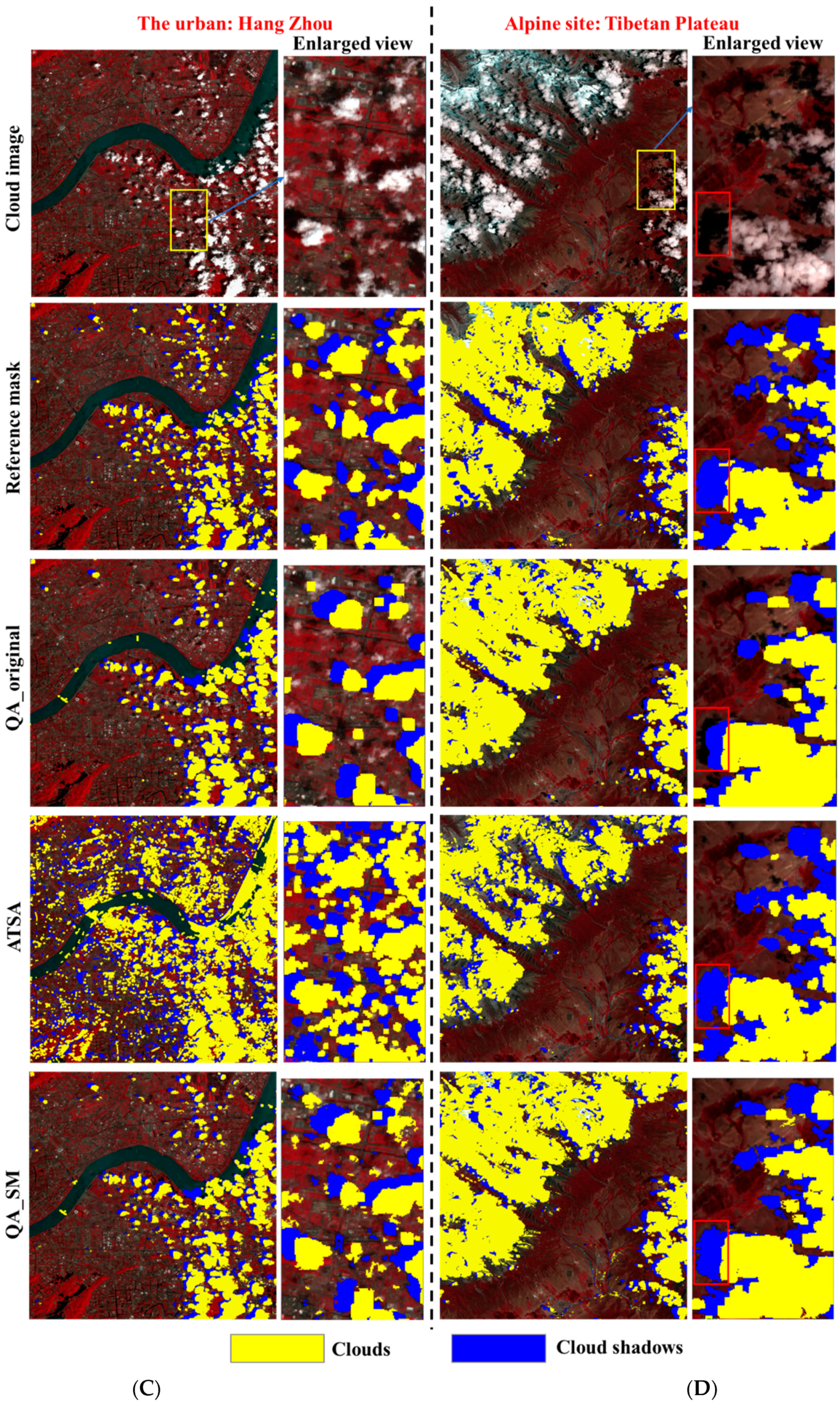
	QA_SM (Reference 2)	11.4%	3.3%	92.4%

summarizes the quantitative assessments for the performance of cloud detection at the four local test sites. Among all methods, QA_SM performed the best with the highest F1-score values at all sites. Compared with the original QA band, QA_SM decreased the omission error effectively but meanwhile, the commission error did not increase even had an extent of decrease. For example, at the site of croplands in the North China Plain, QA_SM decreased the omission error from 5.9% to 3.3% and the commission error from 20.2% to 18.3%. At the urban site of Hangzhou, QA_SM decreased the omission error and the commission error from 27.3% to 17.9% and from 18.9% to 16.3%, respectively. Moreover, the performance of QA_SM was less affected by the different selections of reference images (see “reference 1” and “reference 2” for QA_SM in Table 3), which may be because QA_SM considers the Land surface reflectance changes that are not caused by cloud contamination (i.e., Equations (2) and (7)). Unsatisfactory reference images may be encountered due to temporally continuous cloud contamination. This experiment suggests that QA_SM can be applied to the areas with limited reference images. For the ATSA method, it performed better than QA_original at the forest site in Southeastern China but performed worse than QA_original at the other three sits, particularly at the urban site of Hangzhou with extremely high commission error.

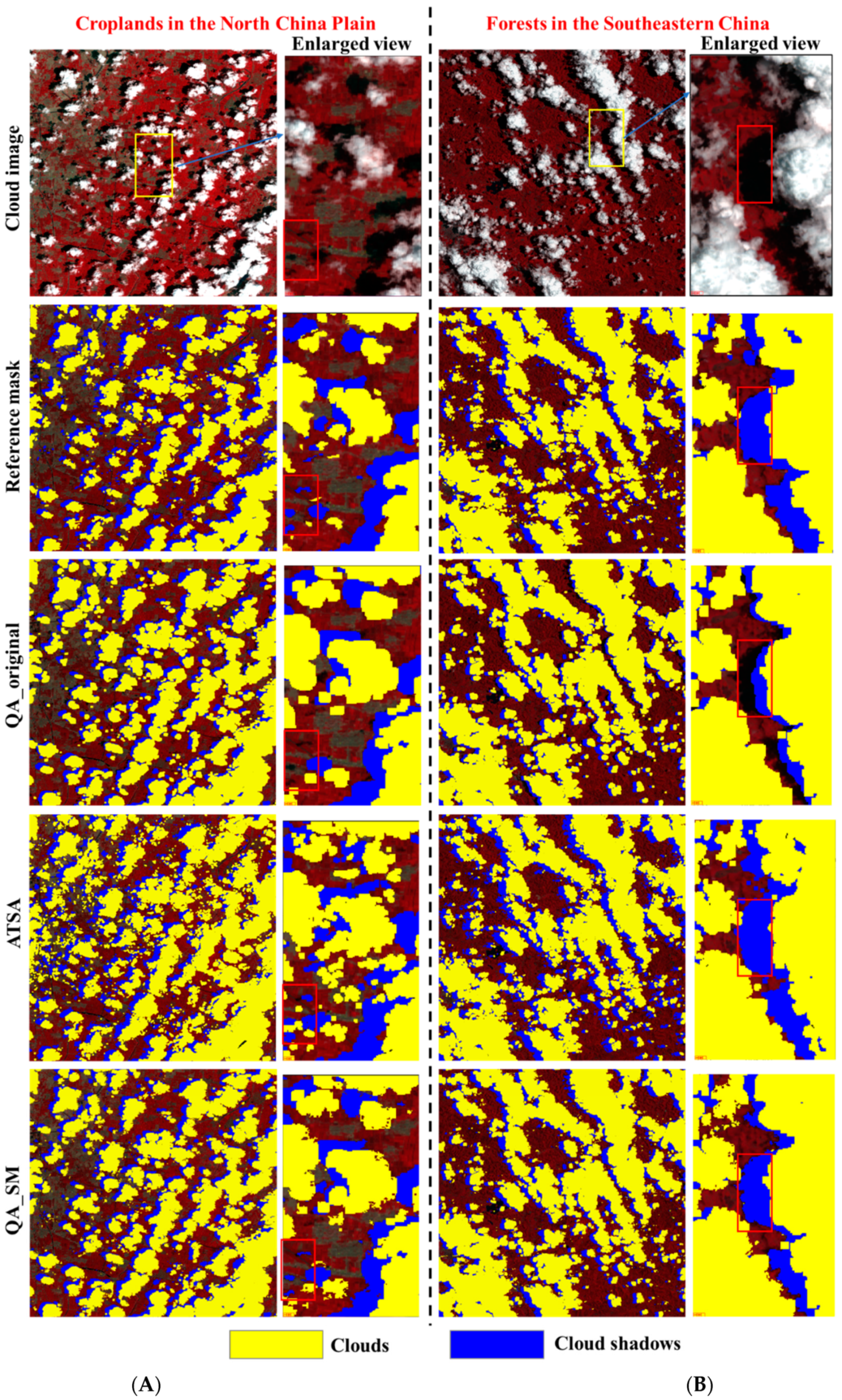
We further show the visual comparisons among different QA bands at the four test sites (Figure 4). It can be seen that QA_original obviously omitted some clouds and cloud shadows, such as the undetected cloud shadows around the edges of some cloud shadow patches (see the enlarged view at the site of Southeastern China, Figure 4B) and those isolated undetected clouds and cloud shadows (see the enlarged view at the site of Hangzhou, Figure 4C). Apparently, the omission error in QA_original is difficult to be corrected by the dilation operations adopted by previous studies. Consistent with the quantitative assessments, QA_SM detected those omitted clouds and cloud shadows effectively even for those small cloud and cloud shadow patches. The performance of ATSA is not stable. Obvious overdetection of clouds and cloud shadows exists at the sites of North China Plain and Hangzhou (Figure 4A,C).

4.1.2. Quantitative Assessments for Cloud Removal by Using Different QA Bands

To test whether the improvement of the QA band can really improve its applications, we performed quantitative assessments for the performance of cloud removal by using different QA bands. The assessments were conducted in six bands, including the blue, green, red, near-infrared, and two short-wave infrared bands (i.e., the bands 2–7 in Landsat 8). Figure 5 shows the RMSE and SSIM values averaged over the six bands when using the LLHM and MNSPI methods to reconstruct cloud-contaminated pixels. In general, QA_SM performed better than QA_original and ATSA with the smallest RMSE values and the highest SSIM values for the reconstructed images. Compared with QA_original, ATSA-derived cloud masks do not always improve the performance of cloud removal. For example, ATSA performed better than the QA_original at the site in the North China Plain whereas performed worse than QA_original at the site in Hangzhou when using MNSPI for cloud removal (Figure 5). At both sites, ATSA decreased the omission error in the cloud mask but has a higher commission error than QA_original, particularly at the site in Hangzhou where the commission error is very high in ATSA (Table 3). This may account for the unstable performance of cloud removal based on the cloud mask of ATSA.

4.2. Experiment II—Evaluations on the Landsat 8 Cloud Cover Validation Dataset

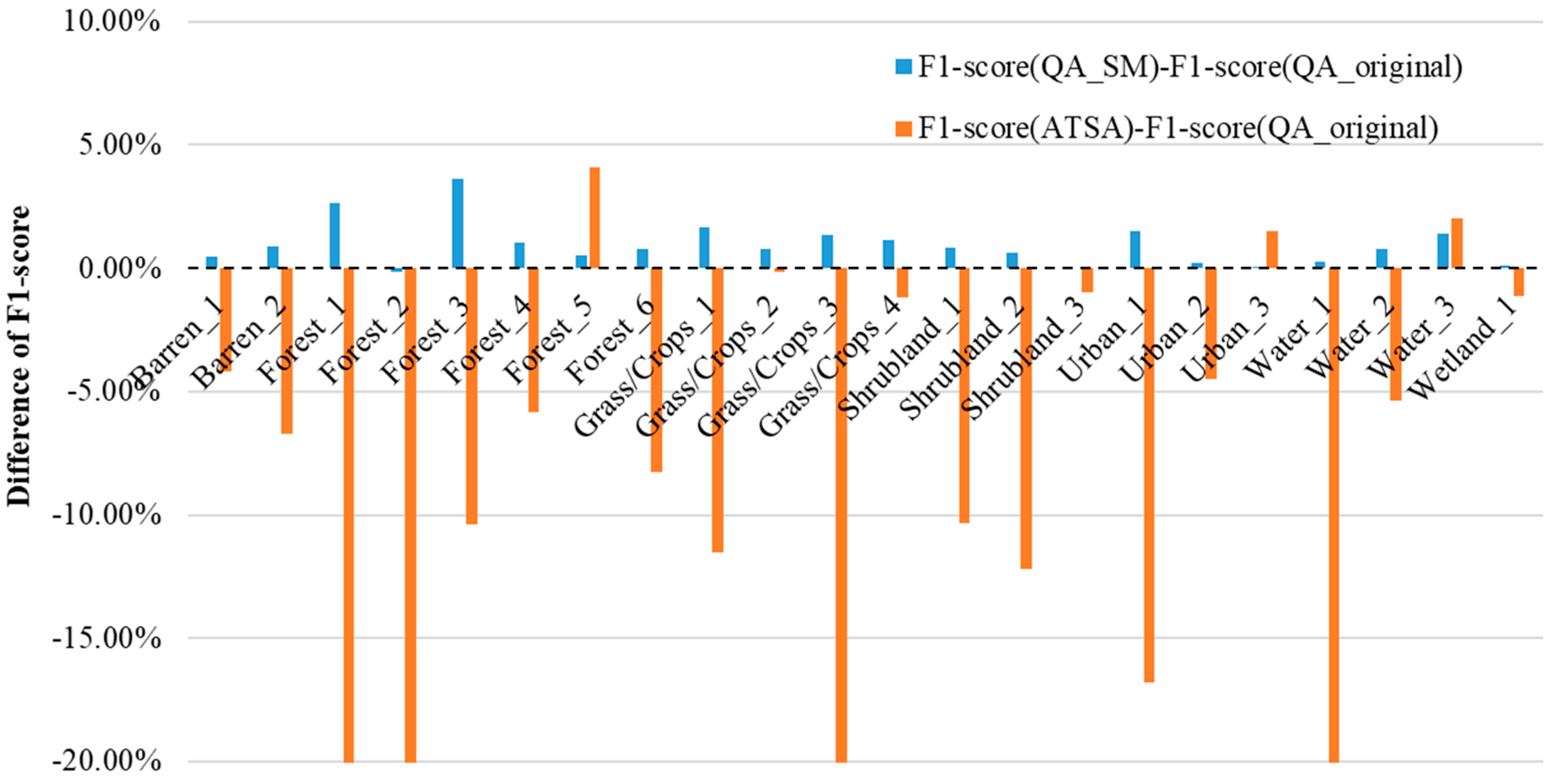
An extensive evaluation was performed on L8_Biome. For intuitive comparisons, Figure 6 highlights the difference in the cloud detection performance between QA_SM and QA_original and that between ATSA and QA_original. Due to page limitations, the detailed evaluation indices at each scene were summarized in Table S1. It can be seen that QA_SM achieved a higher F1-score than QA_original at almost all Landsat scenes. The amplitude of the improvement by QA_SM depends on specific scenes, ranging from 0%–5% in the F1-score (see blue bars in Figure 6). In contrast, ATSA performed worse than QA_original at most scenes (see orange bars in Figure 6). ATSA includes a standard deviation multiplier, a key parameter controlling the balance between commission and omission error (see Equation (6) in [20]). We adopted the recommended value for the standard deviation multiplier in ATSA, but the unstable performance of ATSA may not be due to this parameter setting because ATSA did not show consistent large commission or omission error on L8_Biome (Table S1). In other words, ATSA had a large commission error at some scenes but a large omission error at some other scenes. Regarding the computational efficiency of QA_SM, it took about 10–40 min, depending on the percent of cloud coverage, to detect clouds and cloud shadows for each scene in L8_Biome on a personal computer (CPU: 4-processors with frequency 3.3 GHz).

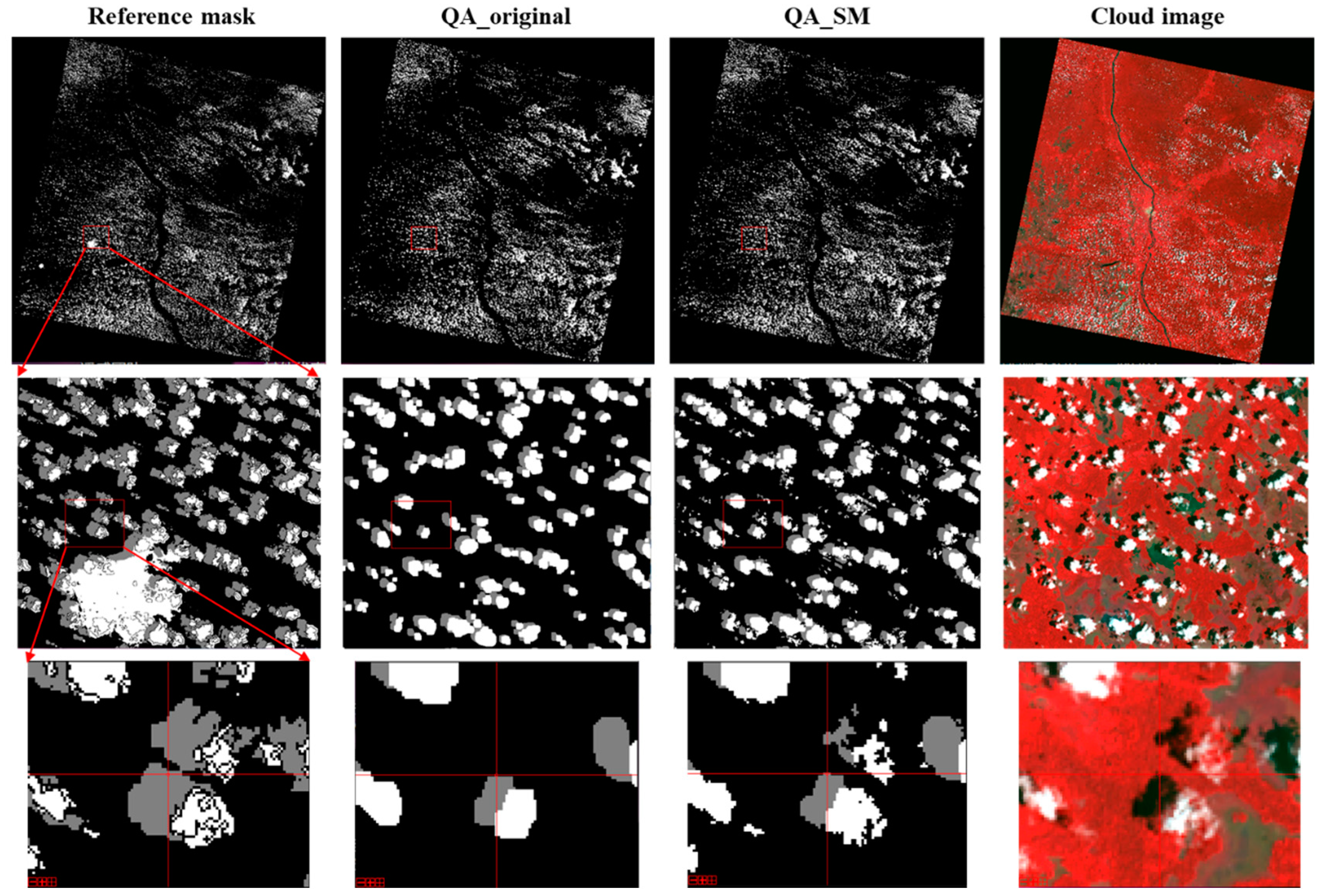
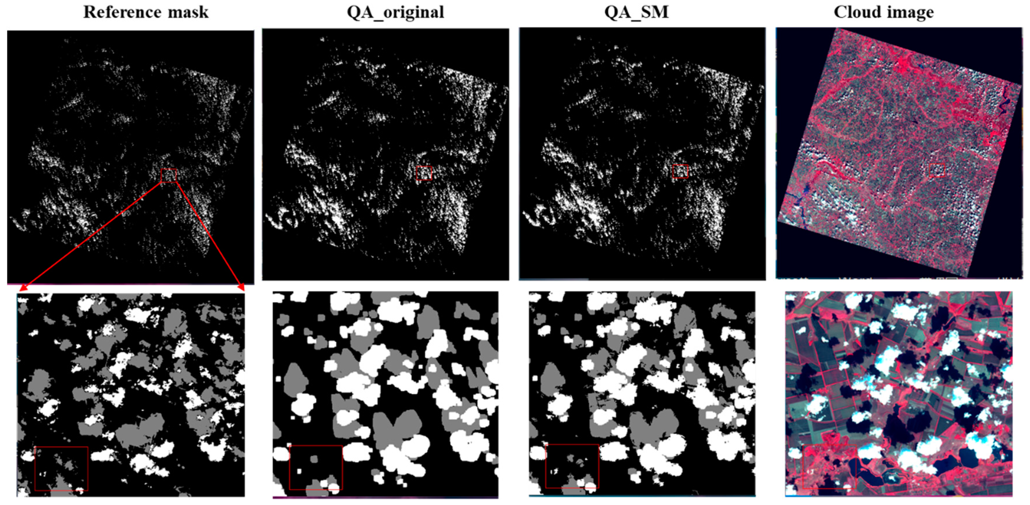
Figure 7, Figure 8, Figure 9 and Figure 10 show the examples for the visual comparisons between the reference mask and different QA bands. Because of the generally poor performance of ATSA (Figure 6), we excluded the visual comparisons for ATSA. We found that QA_SM effectively identified those omitted clouds and cloud shadows around the edges of the original patches (Figure 7) and those isolated clouds and cloud shadows (Figure 8, Figure 9 and Figure 10). Particularly, there may be a large number of clouds and cloud shadows omitted in QA_original in some cases (e.g., see the enlarged view in Figure 9). Such detection errors can be corrected by QA_SM. Interestingly, we found that the reference cloud masks have little commission error but the obvious omission of clouds and cloud shadows in some cases. For example, in the Forest_1 scene, the bare land was incorrectly flagged as clouds (see the panels in the middle row of Figure 8). For the Grass/Crops_1 scene, thin clouds in a large area were not flagged (Figure 9), which could lead to large commission errors for both QA_original and QA_SM. It is worth noting that the generation of manual cloud masks may have a certain subjectivity, particularly for the determination of thin clouds [35]. We suggest further reducing those omitted clouds and cloud shadows in the reference mask by independent analysts.

5. Discussion

Generating cloud and cloud shadow masks are crucial for the applications of various satellite data [36,37]. Landsat QA band still needs to be modified to fulfill the requirement of Landsat image practical applications, such as the reduction of omission error in Landsat QA band for cloud removal in Landsat cloud images [26]. We thus developed a supplementary module to process the original QA band (called QA_SM). Our experiments suggest the effectiveness of the new method. Compared with QA_original (single-temporal method) and ATSA (multi-temporal method), QA_SM performed the best in terms of both visual assessments and quantitative evaluations (Figure 4, Figure 5, Figure 6, Figure 7, Figure 8, Figure 9 and Figure 10).

Two reasons may explain the improvement of the original QA band by QA_SM. First, the original QA band, produced by the Fmask method, is generated by using the single cloud image only. In contrast, to detect cloud pixels, QA_SM considers the high reflectance in the cloud image as well as the reflectance increase between the reference image and the cloud image. Both features of cloud pixels have been quantified by the proposed cloud index (Equation (3)). Similar ideas are adopted by the cloud shadow index in QA_SM for shadows detection (Equation (5)). Compared with those multi-temporal methods based on time-series images, the use of one reference image in QA_SM does not increase more the burden of image collections. Second, considering that Fmask is one of the most accurate single-temporal cloud detection algorithms, QA_SM works based on the original QA band, which not only reduces complexity but improves the robustness of the new method. For example, to reduce the risk of commission error, QA_SM estimated absolute thresholds for clouds and shadows from the original QA band in each Landsat cloud image. Some other operations were also adopted to reduce commission error, such as the geometrical matching between clouds and cloud shadows and the removal of isolated cloud and shadow patches with many small sizes (e.g., <7 pixels). Our results confirmed that QA_SM decreases omission error but meanwhile does not increase commission error in cloud detections, which benefits applications of Landsat cloud images (e.g., cloud removal in Figure 5).

The standard deviation multiplier (i.e., a in Equation (4) and b in Equation (8)) is needed to be determined in QA_SM. Smaller values would be able to detect thinner clouds and lighter cloud shadows. We have tested the parameters at the four experiment sites by varying the values from 1.5 to 2.5 at a step of 0.1. Figure 11 shows the receiver operating characteristic (ROC) curves for the performance of cloud detection. According to the result, we determined this value to be 2.0 by considering the balance between the true positive rate and the false positive rate. Users can tune this value according to different applications. For example, using smaller values to reduce omission errors is expected for the application of cloud removal.

We recognize that some uncertainties remain in our analyses. First, the new version Fmask 4.0 has been developed recently [28], although Landsat QA band is generated by Fmask 3.3. One may wonder whether QA_SM is still useful if Landsat QA band is updated by using Fmask 4.0 in the future. To address this concern, we performed evaluations on L8-Biome again but using Fmask 4.0 to generate the original QA band. Results show that QA_SM still improves the accuracy of the original QA band at most scenes (Figure S2), suggesting the usefulness of QA_SM even if the Landsat QA band is updated by using Fmask 4.0. Second, as a supplementary module to process the original band, QA_SM was compared with the single-temporal method Fmask and the multi-temporal method ATSA. We noted that a large number of methods have been proposed for cloud detection. Till now, Landsat QA band is produced by using Fmask. If the original QA band was produced by using other methods, the effectiveness of QA_SM may be further tested in the future. Third, the requirement of a reference image is likely a limiting factor for the application of the new method. In some regions, such as tropical areas, it may be a challenging task to collect an ideal cloud-free reference image due to temporally continuous cloud contamination. Fourth, to quantitatively evaluate the improvement in the cloud-removal performance by using QA_SM, we simulated reflectance values for clouds and cloud shadows by using MODTRAN. We admit that simulated reflectance values are only the approximations of actual values. However, such simulations are acceptable because locations of clouds and cloud shadows were extracted from another actual Landsat cloud image and MODTRAN was only used for reflectance simulations. Fifth, we employed two cloud-removal methods only (i.e., LLHM and MNSPI) to investigate the influence of cloud detection on the application of cloud removal. However, different cloud-removal methods may have different sensitivity to the quality of the QA band. Such an issue was less considered in previous cloud-removal studies [24]. We recommend taking the quality of the QA band into account when performing comparisons among different cloud-removal methods. Our experimental design based on atmospheric radiative transfer simulation provides a solution to achieve this goal.

6. Conclusions

In this study, we developed a simple method QA_SM to improve the original QA band in the Landsat cloud image. QA_SM combines spectral and geometrical features in the single Landsat cloud image with the temporal change characteristics of clouds and cloud shadows. We compared QA_SM with the single-temporal method Fmask and the multi-temporal method ATSA at four sites of China with different land covers and the Landsat-8 cloud cover validation dataset (“L8_Biome”). By using MODTRAN to simulate reflectance values for clouds and cloud shadows, we further evaluated the performance of cloud removal by using the QA bands generated by different methods. The following conclusions are reached: (1) QA_SM performs better than the Landsat original band and ATSA on both local test sites and L8_Biome with generally higher F1-score values; (2) The better performance of QA_SM is less affected by the selections of reference images. The proposed cloud and cloud shadow indices in QA_SM consider the temporal changes of land surface reflectance that are not caused by cloud contamination; (3) Cloud-removal performance is improved by using QA_SM to process the original QA band, suggesting benefits of QA_SM to advance the applications of Landsat cloud images.

References

- Chen, J.; Liao, A.; Cao, X.; Chen, L.; Chen, X.; He, C.; Han, G.; Peng, S.; Lu, M.; Zhang, W. Global land cover mapping at 30 m resolution: A POK-based operational approach. ISPRS J. Photogramm. Remote Sens. 2015, 103, 7–27. [Google Scholar] [CrossRef] [Green Version]
- Ju, J.; Roy, D.P. The availability of cloud-free Landsat ETM+ data over the conterminous United States and globally. Remote Sens. Environ. 2008, 112, 1196–1211. [Google Scholar] [CrossRef]
- Zhang, X.; Zhou, J.; Liang, S.; Wang, D. A practical reanalysis data and thermal infrared remote sensing data merging (RTM) method for reconstruction of a 1-km all-weather land surface temperature. Remote Sens. Environ. 2021, 260, 112437. [Google Scholar] [CrossRef]
- Wulder, M.A.; Loveland, T.R.; Roy, D.P.; Crawford, C.J.; Masek, J.G.; Woodcock, C.E.; Allen, R.G.; Anderson, M.C.; Belward, A.S.; Cohen, W.B.; et al. Current status of Landsat program, science, and applications. Remote Sens. Environ. 2019, 225, 127–147. [Google Scholar] [CrossRef]
- Hughes, M.J.; Hayes, D. Automated Detection of Cloud and Cloud Shadow in Single-Date Landsat Imagery Using Neural Networks and Spatial Post-Processing. Remote Sens. 2014, 6, 4907–4926. [Google Scholar] [CrossRef] [Green Version]
- Huang, C.; Thomas, N.; Goward, S.N.; Masek, J.G.; Zhu, Z.; Townshend, J.R.G.; Vogelmann, J. Automated masking of cloud and cloud shadow for forest change analysis using Landsat images. Int. J. Remote Sens. 2010, 31, 5449–5464. [Google Scholar] [CrossRef]
- Irish, R.R.; Barker, J.L.; Goward, S.N.; Arvidson, T. Characterization of the Landsat-7 ETM+ Automated Cloud-Cover Assessment (ACCA) Algorithm. Photogramm. Eng. Remote Sens. 2006, 72, 1179–1188. [Google Scholar] [CrossRef]
- Sun, L.; Liu, X.; Yang, Y.; Chen, T.; Wang, Q.; Zhou, X. A cloud shadow detection method combined with cloud height iteration and spectral analysis for Landsat 8 OLI data. ISPRS J. Photogramm. Remote Sens. 2018, 138, 193–207. [Google Scholar] [CrossRef]
- Zhai, H.; Zhang, H.; Zhang, L.; Li, P. Cloud/shadow detection based on spectral indices for multi/hyperspectral optical remote sensing imagery. ISPRS J. Photogramm. Remote Sens. 2018, 144, 235–253. [Google Scholar] [CrossRef]
- Zhu, Z.; Woodcock, C.E. Object-based cloud and cloud shadow detection in Landsat imagery. Remote Sens. Environ. 2012, 118, 83–94. [Google Scholar] [CrossRef]
- Zhu, Z.; Wang, S.; Woodcock, C.E. Improvement and expansion of the Fmask algorithm: Cloud, cloud shadow, and snow detection for Landsats 4–7, 8, and Sentinel 2 images. Remote Sens. Environ. 2015, 159, 269–277. [Google Scholar] [CrossRef]
- Chai, D.; Newsam, S.; Zhang, H.K.; Qiu, Y.; Huang, J. Cloud and cloud shadow detection in Landsat imagery based on deep convolutional neural networks. Remote Sens. Environ. 2019, 225, 307–316. [Google Scholar] [CrossRef]
- Joshi, P.P.; Wynne, R.H.; Thomas, V.A. Cloud detection algorithm using SVM with SWIR2 and tasseled cap applied to Landsat 8. Int. J. Appl. Earth Obs. Geoinf. 2019, 82, 101898. [Google Scholar] [CrossRef]
- Li, W.; Sun, K.; Du, Z.; Hu, X.; Li, W.; Wei, J.; Gao, S. PCNet: Cloud Detection in FY-3D True-Color Imagery Using Multi-Scale Pyramid Contextual Information. Remote Sens. 2021, 13, 3670. [Google Scholar] [CrossRef]
- Ma, N.; Sun, L.; Zhou, C.; He, Y. PCNet: Cloud Detection Algorithm for Multi-Satellite Remote Sensing Imagery Based on a Spectral Library and 1D Convolutional Neural Network. Remote Sens. 2021, 13, 3319. [Google Scholar] [CrossRef]
- Chen, S.; Chen, X.; Chen, J.; Jia, P.; Cao, X.; Liu, C. An Iterative Haze Optimized Transformation for Automatic Cloud/Haze Detection of Landsat Imagery. IEEE Trans. Geosci. Remote Sens. 2015, 54, 2682–2694. [Google Scholar] [CrossRef]
- Goodwin, N.R.; Collett, L.J.; Denham, R.J.; Flood, N.; Tindall, D. Cloud and cloud shadow screening across Queensland, Australia: An auto-mated method for Landsat TM/ETM+ time series. Remote Sens. Environ. 2013, 134, 50–65. [Google Scholar] [CrossRef]
- Hagolle, O.; Huc, M.; Pascual, D.V.; Dedieu, G. A multi-temporal method for cloud detection, applied to FORMOSAT-2, VENµS, LANDSAT and SENTINEL-2 images. Remote Sens. Environ. 2010, 114, 1747–1755. [Google Scholar] [CrossRef] [Green Version]
- Jin, S.; Homer, C.; Yang, L.; Xian, G.; Fry, J.; Danielson, P.; Townsend, P.A. Automated cloud and shadow detection and filling using two-date Landsat imagery in the USA. Int. J. Remote Sens. 2013, 34, 1540–1560. [Google Scholar] [CrossRef]
- Zhu, X.; Helmer, E.H. An automatic method for screening clouds and cloud shadows in optical satellite image time series in cloudy regions. Remote Sens. Environ. 2018, 214, 135–153. [Google Scholar] [CrossRef]
- Zhu, Z.; Woodcock, C.E. Automated cloud, cloud shadow, and snow detection in multitemporal Landsat data: An algorithm designed specifically for monitoring land cover change. Remote Sens. Environ. 2014, 152, 217–234. [Google Scholar] [CrossRef]
- Lin, C.-H.; Lin, B.-Y.; Lee, K.-Y.; Chen, Y.-C. Radiometric normalization and cloud detection of optical satellite images using invariant pixels. ISPRS J. Photogramm. Remote Sens. 2015, 106, 107–117. [Google Scholar] [CrossRef]
- Foga, S.; Scaramuzza, P.L.; Guo, S.; Zhu, Z.; Dilley, R.D.; Beckmann, T.; Schmidt, G.L.; Dwyer, J.L.; Joseph Hughes, M.; Laue, B. Cloud detection algorithm comparison and validation for operational Landsat data products. Remote Sens. Environ. 2017, 194, 379–390. [Google Scholar] [CrossRef] [Green Version]
- Shen, H.; Li, X.; Cheng, Q.; Zeng, C.; Yang, G.; Li, H.; Zhang, L. Missing Information Reconstruction of Remote Sensing Data: A Technical Review. IEEE Geosci. Remote Sens. Mag. 2015, 3, 61–85. [Google Scholar] [CrossRef]
- Cao, R.; Chen, Y.; Chen, J.; Zhu, X.; Shen, M. Thick cloud removal in Landsat images based on autoregression of Landsat time-series data. Remote Sens. Environ. 2020, 249, 112001. [Google Scholar] [CrossRef]
- Zhang, Q.; Yuan, Q.; Li, J.; Li, Z.; Shen, H.; Zhang, L. Thick cloud and cloud shadow removal in multitemporal imagery using progressively spatio-temporal patch group deep learning. ISPRS J. Photogramm. Remote Sens. 2020, 162, 148–160. [Google Scholar] [CrossRef]
- Luo, Y.; Trishchenko, A.; Khlopenkov, K. Developing clear-sky, cloud and cloud shadow mask for producing clear-sky composites at 250-meter spatial resolution for the seven MODIS land bands over Canada and North America. Remote Sens. Environ. 2008, 112, 4167–4185. [Google Scholar] [CrossRef]
- Qiu, S.; Zhu, Z.; He, B. Fmask 4.0: Improved cloud and cloud shadow detection in Landsats 4–8 and Sentinel-2 imagery. Remote Sens. Environ. 2019, 231, 111205. [Google Scholar] [CrossRef]
- Cao, R.; Chen, Y.; Shen, M.; Chen, J.; Zhou, J.; Wang, C.; Yang, W. A simple method to improve the quality of NDVI time-series data by integrating spa-tiotemporal information with the Savitzky-Golay flter. Remote Sens. Environ. 2018, 217, 244–257. [Google Scholar] [CrossRef]
- Wang, Z.; Bovik, A.C.; Sheikh, H.R.; Simoncelli, E.P. Image quality assessment: From error visibility to structural similarity. IEEE Trans. Image Process. 2004, 13, 600–612. [Google Scholar] [CrossRef] [PubMed] [Green Version]
- Berk, A.; Bernstein, L.; Anderson, G.; Acharya, P.; Robertson, D.; Chetwynd, J.; Adler-Golden, S. MODTRAN Cloud and Multiple Scattering Upgrades with Application to AVIRIS. Remote Sens. Environ. 1998, 65, 367–375. [Google Scholar] [CrossRef]
- Scmmuzza, P.; Micijevic, E.; Chander, G. SLC gap-filled products: Phase one methodology on USGS. Landsat Tech. Notes 2004. Available online: https://www.usgs.gov/media/files/landsat-7-slc-gap-filled-products-phase-one-methodology (accessed on 25 November 2021).
- Zhu, X.L.; Gao, F.; Liu, D. A Modifed Neighborhood Similar Pixel Interpolator Approach for Removing Thick Clouds in Landsat Images. IEEE Geosci. Remote Sens. Lett. 2012, 9, 521–525. [Google Scholar] [CrossRef]
- Zhang, Y.; Guindon, B.; Cihlar, J. An image transform to characterize and compensate for spatial variations in thin cloud contamination of Landsat images. Remote Sens. Environ. 2002, 82, 173–187. [Google Scholar] [CrossRef]
- Skakun, S.; Vermote, E.F.; Artigas, A.E.S.; Rountree, W.H.; Roger, J.-C. An experimental sky-image-derived cloud validation dataset for Sentinel-2 and Landsat 8 satellites over NASA GSFC. Int. J. Appl. Earth Obs. Geoinf. 2021, 95, 102253. [Google Scholar] [CrossRef]
- Li, Z.; Shen, H.; Li, H.; Xia, G.; Gamba, P.; Zhang, L. Multi-feature combined cloud and cloud shadow detection in GaoFen-1 wide field of view imagery. Remote Sens. Environ. 2017, 191, 342–358. [Google Scholar] [CrossRef] [Green Version]
- Li, Z.; Shen, H.; Cheng, Q.; Liu, Y.; You, S.; He, Z. Deep learning based cloud detection for medium and high resolution remote sensing images of different sensors. ISPRS J. Photogramm. Remote Sens. 2019, 150, 197–212. [Google Scholar] [CrossRef] [Green Version]
Figure 1.
An illustration showing the geometrical matching between the cloud patch and its shadow patch. is the horizontal distance between a cloud patch j and its shadow patch.
Figure 2.
An example showing the generation of the cloud-simulated image at the site of the North China Plain. (A) The actual cloud image; (B) The reference mask of the actual cloud image was overlapped on a cloud-free image. The yellow and blue polygons indicate the locations of clouds and cloud shadows; (C) The reflectance values of clouds and cloud shadows in (B) were simulated by MODTRAN (For details, please refer to Section 3.1.2). Noted: the site of North China Plain is covered by croplands (i.e., red color in (C)) and built-up regions (i.e., cyan color in (C)).
Figure 3.
A sketch showing the simulations for cloud pixels and cloud shadow pixels by MODTRAN.
Figure 4.
The QA bands generated by different methods at (A) croplands in North China Plain, (B) forests in the Southeastern China, (C) Hangzhou urban, and (D) alpine grasslands in Tibetan plateau.
Figure 5.
The RMSE values and SSIM values for cloud-removal performance on the cloud-simulated images when using the LLHM and MNSPI method. Values are averaged over six bands.
Figure 6.
The difference of F1-score between QA_SM and QA_original (blue color) and between ATSA and QA_original (orange color) at each L8_Biome scene. A negative (positive) value suggests a worse (better) performance of the method than QA_original. For information on each scene, please refer to Table 2.
Figure 7.
Visual comparisons among the reference cloud mask, QA_original, QA_SM, and the cloud image (standard false color composition) at Barren_1. Clouds and cloud shadows are represented by white and gray color. The lower row shows enlarged views.
Figure 8.
The same as Figure 7 but for the Forest_1 scene. The lower rows show the enlarged view (see the “reference mask” column).
Figure 9.
The same as Figure 7 but for the Grass/Crops_1 scene.
Figure 10.
The same as Figure 7 but for the Urban_1 scene.
Figure 11.
The receiver operating characteristic (ROC) curves for the performance of cloud detections in experiment II. The standard deviation multiplier (i.e., a in Equation (4) and b in Equation (8)) varies from 1.5 to 2.5 at a step of 0.1. TPR-true positive rate; FPR-false positive rate.